B VIOLATION IN THE HOT STANDARD MODEL

I explain, as simply and pedagogically as I can, recent arguments that the high-temperature baryon number violation rate depends on the electroweak coupling as $\Gamma=\#\alpha_{\rm w}^{5}T^{4}$ (up to higher order corrections). This is in contrast to the form $\Gamma=\#\alpha_{\rm w}^{4}T^{4}$ that has historically been assumed in discussions of electroweak baryogenesis. I will give a general analysis of the time scale for non-perturbative gauge field fluctuations in hot non-Abelian plasmas.

1 Introduction

I will be discussing baryon number (B) violation in the Standard Model in the hot, early universe. The motivation is scenarios of electroweak baryogenesis, which typically depend on the rate $\Gamma$ of B violation in the hot, symmetric phase of electroweak theory. The particular focus of my discussion will be to understand what physics determines the size of $\Gamma$ and to understand how $\Gamma$ depends on the parameters of the theory.

The source of B violation is the electroweak anomaly for baryon number, which demands that

$$\Delta B\sim g_{\rm w}^{2}\int dt\;d^{3}x\>{\rm tr}F_{\rm w}\tilde{F}_{\rm w}.$$ (1)

The subscript “w” (often suppressed in the following) indicates that the coupling is the weak coupling and the field strengths those of the weak gauge fields. This anomaly equation relates the amount of B violation to topological transitions in the weak gauge fields. I shan’t review the anomaly any further but will just take (1) as my starting point.

The problem of understanding the size of the B violation rate can be simplified a bit. Because the physics of interest is the B violation rate in the hot, symmetric phase of electroweak theory, the Higgs field doesn’t play any essential role. So I shall ignore the Higgs field altogether. In addition, even though the behavior of the fermions is the ultimate matter of interest, fermions don’t actually play an essential role in determining the rate. The anomaly (1) tells us that fermion number violation is a consequence of what the gauge fields are doing: If the gauge fields have non-trivial $g^{2}\int F\tilde{F}$, then B violation will tag along as a consequence. As long as couplings are small, the back-reaction of the fermions on the gauge-field dynamics turns out to be a higher-order effect. So one can forget about the fermions and analyze the following, simplified problem: 

What’s the rate of topological transitions in pure SU₂ gauge theory at high temperature?

By dimensional analysis, the rate per unit volume at high temperature must depend on temperature as $T^{4}$. But what is the dependence on $\alpha_{\rm w}$? The purpose of this talk is to explain a relatively recent analysis by myself, Dam Son, and Larry Yaffe $\!{}^{{\bf?}}$ that, in weak coupling ($\alpha_{\rm w}\to 0$), the B violation rate behaves as

$$\Gamma\equiv{\hbox{rate}\over\hbox{volume}}=\#\alpha_{\rm w}^{5}T^{4}.$$ (2)

In contrast, it has instead long been assumed in the literature that $\Gamma=\#\alpha_{\rm w}^{4}T^{4}$. I shall explain later the origin of this belief.

2 The scales of the problem

Because of the factor of $g^{2}$ in the anomaly equation (1), it follows that $\Delta B$ of order 1 requires non-perturbatively large field strengths of order $1/g$. The energy of the intermediate gauge configurations in a B-violating process will therefore also be non-perturbatively large and of order $1/g^{2}$. The moral to keep in mind in everything that follows is that non-perturbatively large amplitude fluctuations are required for a topological transition.

Figure 1: A schematic representation of the (bosonic) potential energy along a particular direction (labeled $z$) in field space, corresponding to topologically non-trivial transitions between vacua. $N_{\rm cs}$ labels the Chern-Simmons number corresponding to the different large gauge transformations of the $\vec{A}=0$ vacuum.

Now consider fig. 1, which is a very rough depiction of the potential energy in gauge configuration space (and is required by international law to be shown in every talk on electroweak B violation). The horizontal axis depicts one particular direction in the infinite-dimensional space of gauge field configurations $\vec{A}(x)$. (I’m working for the moment in $A_{0}=0$ gauge.) The vertical axis corresponds to the potential energy of those configurations. The minima correspond to the perturbative vacuum $\vec{A}=0$ and large gauge transformations of it, and you can think of the configurations inbetween as those that a particular process passes through when violating B through the anomaly. There is therefore an energy barrier $E_{\rm barrier}$ of order $1/g^{2}$ for such processes. At non-zero temperature, one expects that the probability for the system to have enough energy to pass over this energy barrier is given roughly by a Maxwell-Boltzmann factor,

$$\Gamma\sim\exp\left(-\beta E_{\rm barrier}\right),$$ (3)

where $\beta$ is the inverse temperature.

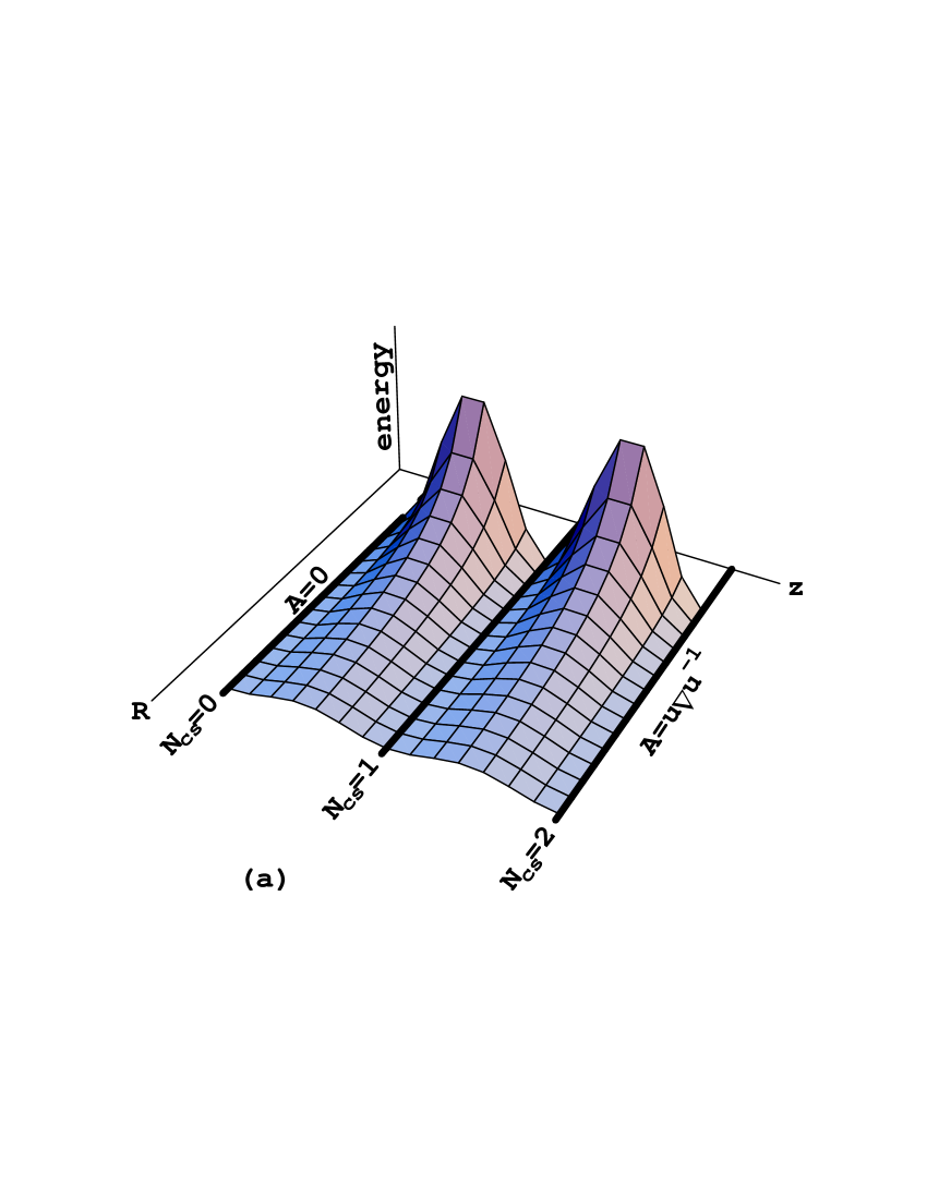
Figure 2: The same as fig. 1 but supplemented by an extra dimension of configuration space corresponding to the spatial size $R$ of the configurations.

So far I’ve discussed the dependence of the fields and energy barrier on coupling $g$, but I haven’t explained what sets the dimensionful scale for these quantities. Pure gauge theory is (at least classically) scale invariant. If the gauge configurations responsible for a topological transition have spatial size $L$, then $L$ is the only thing that can set the scales. $\Delta B\sim 1$ then implies

$$F_{\rm barrier}\sim{1\over gL^{2}},\qquad A_{\rm barrier}\sim{1\over gL},\qquad E_{\rm barrier}\sim{1\over g^{2}L}.$$ (4)

To capture the most important qualitative features of the gauge configuration potential energy, we should really supplement Fig. 1 by one additional direction in gauge configuration space, representing the spatial size $L$ of configurations. This gives Fig. 2, where the energy barrier has now become a ridge. As given by (4), transitions through very small configurations are associated with a high energy barrier, while transitions through arbitrarily large configurations are associated with an arbitrarily small barrier. The transition probability

$$\Gamma\sim\exp(-\beta E_{\rm barrier})\sim\exp(-\#/g^{2}LT)$$ (5)

is unsuppressed when $L\mathrel{\mathchoice{\lower 3.0pt\vbox{\halign{$\m@th\displaystyle\hfill#\hfil$\cr>\crcr\sim\crcr}}}{\lower 3.0pt\vbox{\halign{$\m@th\textstyle\hfill#\hfil$\cr>\crcr\sim\crcr}}}{\lower 3.0pt\vbox{\halign{$\m@th\scriptstyle\hfill#\hfil$\cr>\crcr\sim\crcr}}}{\lower 3.0pt\vbox{\halign{$\m@th\scriptscriptstyle\hfill#\hfil$\cr>\crcr\sim\crcr}}}}1/g^{2}T$. In fact, $L\sim 1/g^{2}T$ is the dominant scale associated with transitions. This is due to entropy: there are a lot more short-distance modes than long-distance modes. As a result, transitions are dominated by the shortest distance scale $L$ that is unsuppressed.

$$\matrix{\hbox{Dominant spatial scale:}\hfill&L\sim 1/g^{2}T\hfill\cr\hbox{Dominant momentum scale:}\hfill&k\sim g^{2}T\hfill\cr}$$ (6)

This is, more generally, the scale for any unsuppressed, non-perturbative, colored fluctuations.

We can now understand the naive rate estimate that has previously been used in the literature. In a relativistic theory of massless particles, one might expect time scales to be the same as distance scales, so that

$$t\sim L\sim{1\over g^{2}T}\,.\qquad\qquad\hbox{~{}~{}~{}~{}(naive)}$$ (7)

A rate of one unsuppressed transition per volume $L^{3}$ per time $t$ then gives

$$\Gamma\sim{1\over L^{3}t}\sim g^{8}T^{4}.\qquad\qquad\hbox{(naive)}$$ (8)

This would predict $\Gamma=\#\alpha^{4}T^{4}$ where $\#$ is a constant that cannot be computed in perturbation theory (since the gauge fluctuations are non-perturbative).

The problem with the above estimate is that finite temperature physics is not Lorentz invariant. There is a preferred frame: the rest frame of the plasma. As a result, one cannot assume that time scales will be the same as distance scales. In particular, Son, Yaffe and I have argued that viscous forces in the plasma slow down the dynamics of the long-distance ($L\sim 1/g^{2}T$) modes. As I shall discuss, we find that the time scale is slowed down to $t\sim 1/g^{4}T$.

$$\matrix{\hbox{Dominant time scale:}\hfill&t\sim 1/g^{4}T\hfill\cr\hbox{Dominant frequency scale:}\hfill&\omega\sim g^{4}T\hfill\cr}$$ (9)

As a result, the rate $\Gamma\sim 1/tL^{3}$ is then

$$\Gamma=\#\alpha^{5}T^{4}\,,$$ (10)

where $\#$ is again a non-perturbative constant.

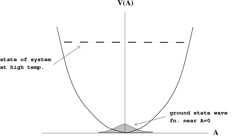
Figure 3: A slightly anharmonic oscillator. High-energy states probe non-perturbatively large amplitudes.

3 Why high T generically creates non-perturbatively large amplitude fluctuations

I’d now like to explain very generally why physics becomes non-perturbative at high temperature, even in theories that are weakly coupled ($g\ll 1$). As a simple example, consider a very simple problem from quantum or classical mechanics: a very slightly anharmonic oscillator. The Lagrangian is simply

$$L\sim\dot{\phi}^{2}-V(\phi),\qquad\qquad V(\phi)\sim m^{2}\phi^{2}+g^{2}\phi^{4}.$$ (11)

At zero temperature and low energies, the states of interest are the ground state wave function and its low-lying excitations. The wave function is localized near $\phi=0$, and the anharmonic term in the potential can be treated as a perturbation. At arbitrarily high temperature, however, the system occupies states of arbitrarily high energy, which are states that probe arbitrarily large amplitudes of $\phi$. But, for large enough $\phi$, a quartic term $g^{2}\phi^{4}$ will always dominate over a quadratic one $m^{2}\phi^{2}$, no matter how small $g$ is. The situation is depicted schematically in Fig. 3.

To estimate when perturbation theory breaks down, first pretend the anharmonic term can indeed be treated perturbatively. For a harmonic oscillator, the amplitude of $\phi$ at high temperature is given by the equipartition theorem:

$$m^{2}\phi^{2}\sim T\qquad\qquad\Longrightarrow\qquad\qquad\phi^{2}\sim{T\over m^{2}}.$$ (12)

A measure of whether $\phi$ is perturbative is given by the ratio of the anharmonic to harmonic terms:

$$1{\buildrel?\over{\gg}}{g^{2}\phi^{4}\over m^{2}\phi^{2}}\sim{g^{2}T\over m^{4}}\,.$$ (13)

The thing to keep in mind is that large $T$, or equivalently small $m$, implies large, non-perturbative amplitudes $\phi$. Conversely, small $T$ or large $m$ implies small, perturbative amplitude fluctuations in $\phi$.

The field theory versions of (12) and (13) look quite similar, with the natural frequency $m$ of the oscillator replaced by $\omega_{k}$, where $k$ is the spatial momentum characteristic of the modes of interest. Specifically, the amplitude analogous to (12) is

$$\left[(\bar{\phi})_{L}\right]^{2}\sim{T\over\omega_{k}^{2}L^{3}}$$ (14)

where $(\bar{\phi})_{L}$ represent $\phi$ smeared (i.e. averaged) over a spatial scale of order $L$ and where

$$k\sim 1/L.$$ (15)

The perturbative condition analogous to (13) is

$$1{\buildrel?\over{\gg}}{g^{2}T\over\omega_{k}^{4}L^{3}}.$$ (16)

The amplitude of fluctuations will be perturbative on every distance scale $L$ if

$$1{\buildrel?\over{\gg}}\max_{L}\left(g^{2}T\over\omega_{k}^{4}L^{3}\right)\sim{g^{2}T\over m}.$$ (17)

People familiar with high-temperature perturbation theory will recognize this as the standard condition for the ultimate success of perturbation theory.

Figure 4: Forward scattering of a mode of interest (solid line) off of a particle in the plasma (dashed line) in $\phi^{4}$ theory.

4 The last section is a lie

The last section suggested that non-perturbative amplitudes are generic at very high temperature. In fact, in field theories, the opposite is true: amplitudes generically remain perturbative. The reason is that interactions in field theory can cause the effective mass of modes to change at high temperature:

$$m\qquad\longrightarrow\qquad m_{\rm eff}(T).$$ (18)

This change in the effective mass is caused by the forward scattering of propagating modes off of particles in the thermal bath. This forward scattering modifies the effective propagation of the modes in a way that can change their effective mass. For definiteness, consider $\phi^{4}$ theory. The leading-order forward-scattering amplitude is shown in Fig. 4, where the solid line denotes the mode of interest and the dashed line represents a particle present in the thermal bath. As far as the mode of interest is concerned, such a process looks just like a mass insertion, and it turns out to give

$$m_{\rm eff}^{2}\sim g^{2}T^{2}.$$ (19)

But this effective mass is large enough at high $T$ that $\phi$ remains perturbative! The perturbative expansion parameter (17) becomes

$${g^{2}T\over m_{\rm eff}}\sim g,$$ (20)

which is indeed small if the theory is weakly coupled.

Figure 5: Forward scattering of a mode of interest (wavy line) off of a particle in the plasma (dashed line) in gauge theory. the particle in the plasma might be anything—a gauge boson, scalar, or fermion.

5 Gauge theory

Now let’s consider gauge theory. The leading-order processes for forward scattering are shown in Fig. 5, where the dashed line represents any sort of particle in the thermal bath—gauge, scalar, or fermion—that the gauge mode of interest scatters off of. We’d like to know what sort of effective thermal mass, or more generally what sort of self-energy $\Pi(\omega,k)$, is generated by this forward scattering. To physically motivate the result, it will be useful to first review some basic features of plasmas. Think back to your graduate electrodynamics course and a book like Jackson.

• Debye screening of electric fields. Static electric fields are screened in a plasma because the charged particle in the plasma re-arrange themselves. In the case at hand, this manifests as

  $$\Pi_{\rm L}(\omega,k)=O(g^{2}T^{2})\qquad\hbox{for}\qquad\omega=0\qquad\qquad(k\ll T).$$ (21)

  That is, the self-energy has an effective mass in the static limit $(\omega=0)$. The subscript ${\rm L}$ denotes the “longitudinal” polarization of the gauge field, which is the polarization corresponding to electric fields in the static limit (polarization $A_{0}$ for $\omega=0$ in covariant gauge). The $T^{2}$ in (21) comes from dimensional analysis in the ultrarelativistic limit, and the $g^{2}$ comes from the interactions in fig. 5.

• No screening of static magnetic fields. Unlike electric fields, static magnetic fields are not screened in a plasma, and

  $$\Pi_{\rm T}(\omega,k)=0\qquad\hbox{for}\qquad\omega=0\qquad\qquad(k\ll T).$$ (22)

  There is no effective mass. The subscript ${\rm T}$ denotes the two “transverse” polarizations—those which correspond to magnetic fields in the static limit. Sometimes, people speak loosely of a “magnetic screening mass” in hot non-Abelian gauge theories. This is somewhat misleading language, however: magnetic fields actually become strong and confining at large distances.

• Plasma frequency for propagating waves. In a QED plasma, propagating electromagnetic waves have a minimum frequency. This frequency gap is known as the plasma frequency (or the plasmon mass). In our case, the plasma frequency, and in fact the frequency of all low-momentum $(k\ll T)$, propagating, colored modes, is of order

  $$\Pi_{{\rm L},{\rm T}}(\omega,k)=O(g^{2}T^{2})\qquad\hbox{for}\qquad\omega>k\qquad\qquad(\omega,k\ll T).$$ (23)

There is an exact formula $\!{}^{{\bf?}}$ for the one-loop self-energy of Fig. 5, the details of which won’t be necessary for this discussion. A simple summary of the relevant features, which incorporate the various limits discussed above, is

$$\Pi_{\rm L} = g^{2}T^{2}\cases{O(1)-iO\left(\omega\over k\right),&~{}~{}~{}~{}$\omega\ll k$ ,\cr O(1),&~{}~{}~{}~{}$\omega\geq k$ ;\cr}$$

$$\Pi_{\rm T} = g^{2}T^{2}\cases{O\left(\omega^{2}\over k^{2}\right)-iO\left(\omega\over k\right),&$\omega\ll k$ ,\cr O(1),&$\omega\geq k$ .\cr}$$ (24)

Note that $\Pi$ has an imaginary part  for $\omega<k$, which I’ll explain below, and that this imaginary part dominates $\Pi_{\rm T}$ when $\omega\ll k$.

We’re now in a position to see the problem with the original assumption in the literature that the time scale for topological transitions is $t\sim 1/g^{2}T$ so that the rate is $\Gamma\sim\alpha^{4}T^{4}$. The naive assumption $t\sim L$ is $\omega\sim k$ in frequency space. But then (24) gives $\Pi\sim g^{2}T^{2}$, which is basically determined by having to reproduce the plasma frequency effect. However, $\Pi\sim g^{2}T^{2}$ is the same as the scalar $\phi^{4}$ theory case discussed in the last section, which we learned only produces perturbatively small fluctuations in field amplitude. So $t\sim 1/g^{2}T$ cannot be the time scale for the non-perturbative gauge-field fluctuations required for a topological transition.

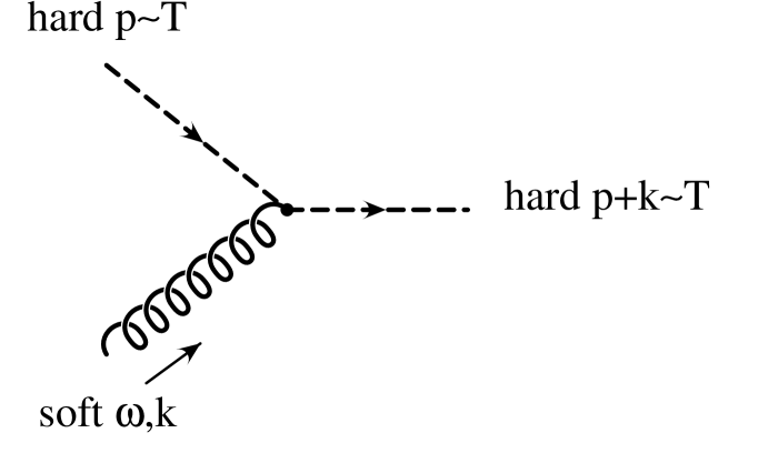
Figure 6: The absorption of a soft excitation (wavy line) by the small-angle scattering of a hard excitation (dashed line).

Our only hope is to make the effective mass of fluctuations substantially smaller than $\Pi\sim g^{2}T^{2}$. Now remember that $\Pi$ vanishes for static magnetic fields; so it can be made arbitrarily small by considering nearly static magnetic fields. Eq. (24) gives

$$\Pi_{\rm T}\sim-ig^{2}T^{2}{\omega\over k}\qquad\qquad(\omega\ll k).$$ (25)

This can also be written as

$$\Pi_{\rm T}\sim{g^{2}T^{2}\over k}\,\partial_{t}.$$ (26)

This appears as a damping term in the effective equations of motion for the gauge field. The physical origin of this damping is the process shown in fig. 6. Low-momentum, space-like quanta corresponding to nearly-static magnetic fields can be absorbed by particles in the plasma, with a resulting loss of energy from the magnetic fields of interest.

Most of the particles in the plasma have large momenta $p\sim T\gg g^{2}T$. The damping effect just discussed for low-momentum magnetic fields is indeed dominated by the contribution from absorption by high-momentum particles.

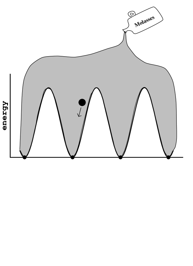
Figure 7: Similar to fig. 1 except now the dynamics of the long-distance modes of interest is slowed down by hot molasses.

6 A non-linear pendulum in hot molasses

As just discussed, the short-distance modes ($p\sim T$) in the plasma cause damping of the dynamics of the long-distance modes ($k\sim g^{2}T$) of interest for topological transition. A fairly good analogy is that the long-distance modes are like a ball rolling around in a potential that has been filled with hot molasses, as depicted in fig. 7, where the molasses represents the effect of the short-distance modes. In fact, this analogy is useful enough that it is worth forgetting about gauge theory for a moment and reviewing the physics of a slightly non-linear pendulum in hot molasses.

Consider the motion of a slightly non-linear pendulum—that is, the behavior near the bottom of one of the wells in fig. 7:

$$(\partial_{t}^{2}+k^{2})A+O(A^{2})=0.$$ (27)

For a pendulum in (idealized) hot molasses, this equation should be modified to a Langevin equation of the form

$$(\partial_{t}^{2}+\gamma\partial_{t}+k^{2})A+O(A^{2})=\xi(t).$$ (28)

A damping term, with some coefficient $\gamma$, has been added on the left side to represent the viscous drag of the molasses. If the molasses is hot, then random thermal fluctuations of the molasses will randomly buffet the pendulum. This effect is represented by a random force term $\xi(t)$ on the right-hand side.

Non-perturbative physics corresponds to large-amplitude fluctuations of the pendulum, so that the non-linear terms in (28) become important. Let’s estimate the time scales involved by first ignoring the non-linearities and finding the time scale for the largest amplitude fluctuations of a simple harmonic oscillator in hot molasses.

The damping of the pendulum and the random force term are both due to interactions with the molasses, and so their strength is related. More precisely, the two are related by the fluctuation-dissipation theorem, whose consequence in this case (ignoring non-linear interactions) is that the random force has a white-noise spectrum normalized to

$$\langle\xi(t)\xi(t^{\prime})\rangle=2\gamma T\delta(t-t^{\prime})\,.$$ (29)

Note that the magnitude is proportional to both the damping and the temperature. The response of the oscillator (28) to this force is easy to solve by Fourier transform:

$$A(\omega)={\xi(\omega)\over-\omega^{2}-i\gamma\omega+k^{2}}\,.$$ (30)

Using (29), the power spectrum of amplitude fluctuations is then

$$\langle A(\omega)^{*}A(\omega)\rangle={2\gamma T\,\delta(\omega-\omega^{\prime})\over|-\omega^{2}-i\gamma\omega+k^{2}|^{2}}.$$ (31)

Figure 8: A schematic plot of the power of amplitude fluctuations for an oscillator in idealized molasses.

Now let’s specialize to the case of a strongly damped pendulum, where the damping coefficient $\gamma$ is large compared to the natural frequency $k$. The behavior of (31) is shown in Fig. 8: there are small amplitude fluctuations at high frequency and larger amplitude fluctuations at low frequency. The largest amplitude fluctuations are when the denominator in (31) becomes small at low frequency. The $\omega^{2}$ term in the denominator can then be ignored, and the characteristic frequency $\omega_{\rm c}$ of the largest amplitude fluctuations comes from equating the magnitudes of the $-i\gamma\omega$ and $k^{2}$ terms:

$$\omega_{\rm c}\sim{k^{2}\over\gamma}\ll k,$$ (32)

where the last inequality follows from the assumption $\gamma\gg k$ of strong damping. Note that $\omega\ll k$ is precisely the kinematic regime of slowly varying fields that we’ve already discussed as being important for non-perturbative physics in gauge theory.

7 Back to Hot Gauge Theory

In hot gauge theory, the effective equation for the long-distance modes is

$$(-\omega^{2}+\Pi(\omega,k)+k^{2})A+O(A^{2})=\xi(\omega,k),$$ (33)

where $\xi$ is a random force caused by interaction with the short-distance modes. For $\omega\ll k$, we reviewed earlier that

$$\Pi(\omega,k)\approx-i\#g^{2}T^{2}{\omega\over k}\equiv\gamma\partial_{t}$$ (34)

for the relevant degrees of freedom, which puts the effective equation precisely in the form of (28). The damping coefficient $\gamma$ is

$$\gamma=\#{g^{2}T^{2}\over k}.$$ (35)

We can now see that the damping is strong. Remember that topological transitions are dominated by spatial momenta $k$ of order $g^{2}T$. Then (35) gives

$$\gamma\sim T\gg k.$$ (36)

The characteristic frequency of large-amplitude fluctuations is then given by (32):

$$\omega_{\rm c}\sim{k^{2}\over\gamma}\sim g^{2}T.$$ (37)

The associated time scale is

$$t\sim{1\over\omega_{\rm c}}\sim{1\over g^{4}T}.$$ (38)

This is the main result of this talk and is precisely the claim I made at the beginning for the time scale relevant to non-perturbative physics such as topological transitions. Using the power spectrum (31), it is possible to check (see ref. 2 for details) that the amplitude of fluctuations associated with $\omega_{\rm c}$ is indeed non-perturbative—that is, that

$$A\sim{1\over gL}\sim gT,$$ (39)

where the first inequality is the condition for non-perturbative fluctuations and the second follows from $L\sim 1/g^{2}T$. Moreover, the fluctuations associated with any larger frequency (shorter time scale) are smaller and therefore perturbative—they cannot be responsible for topological transitions.

Figure 9: A schematic plot of the power of gauge-field fluctuations with $k\sim g^{2}T$. The $\delta$-function spike at $\omega\sim gT$ corresponds to propagating plasmons.

8 Putting the color back into white noise

In the last section, I assumed that the relevant physics involved $\omega\ll k$, which simplified the discussion by making the effective equation of motion (33) look just like the idealized molasses example. I now just want to show that nothing drastic happens to the analysis if we don’t assume $\omega\ll k$ from the beginning but keep the equation in the more general form of (33). There is still a result from the fluctuation-dissipation theorem, whose more general form looks like

$$\langle\xi^{*}\xi\rangle\sim(n_{\omega}+1)\,{\rm Im}\Pi\,$$ (40)

where $n_{\omega}$ is the Bose distribution function. The corresponding response of $A$ may be written as

$$\langle A^{*}A\rangle\sim(n_{\omega}+1)\;{\rm Im}\left(1\over(\omega+i\epsilon)^{2}-k^{2}-\Pi(\omega,k)\right),$$ (41)

where $\epsilon$ is an infinitesimal that selects the retarded response. The resulting power spectrum is shown in fig. 9. (See ref. 2 for details.) For $\omega\ll k$, the result is the same as before; but the spectrum disappears at $\omega=k$. Then at $\omega\sim gT$ there is a $\delta$-function corresponding to the pole of (41), which corresponds to propagating plasma waves. As before, one can check that the fluctuations in $A$ for all frequencies with $\omega\gg g^{4}T$ are only perturbative and cannot be responsible for topological transitions. Non-perturbative physics comes from $\omega\sim g^{4}T$.

9 Conclusions

I’ve tried to argue as pedagogically as possible that the time scale associated with non-perturbative, colored fluctuations of hot gauge fields is $t\sim 1/g^{4}T$ and that the rate for baryon number violation in the hot, symmetric phase of electroweak theory is therefore $\Gamma\sim\alpha_{w}^{5}T^{4}$ at weak coupling. There are a couple of interesting things I haven’t have time to discuss:

• I treated all the effective long-distance equations in linear approximation. In fact, the full non-linear effective equations are known and come from an analysis of what are known as “hard thermal loops.” See ref. 1 for a review and Huet and Son,$\!{}^{{\bf?}}$ as well as Son’s talk in these proceedings.

• This effective long-distance theory is not generally rotationally invariant for classical theories defined on a short-distance lattice, such as those discussed in the talks by Krasnitz and by Moore $\!{}^{{\bf?}}$ for simulating the B violation rate numerically. See ref. 1 and Bodeker et al.$\!{}^{{\bf?}}$ for a discussion. The failure to recover rotational invariance (which may come as a surprise to those readers more familiar with Eucliean-time lattice systems) turns out not to be a complete distaster for using classical lattice simulations to understand the continuum theory.$\!{}^{{\bf?}}$

• It is possible to convert between the rate $\Gamma$ measured in classical lattice simulations and the real $\Gamma$ in quantum field theory. See ref. 1.

References

References

- [1] P. Arnold, University of Washington report UW/PT-97-2, hep-ph/9701393, to appear in Phys. Rev. D.
- [2] P. Arnold, D. Son, and L. Yaffe, Phys. Rev. D 55, 6264 (1997).
- [3] H. Weldon, Phys. Rev. D 26, 1394 (1982); U. Heinz, Ann. Phys. (N.Y.) 161, 48 (1985); 161, 48 (1985); 168, 148 (1986).
- [4] P. Huet and D. Son, Phys. Lett. B 393, 94 (1997).
- [5] A. Krasnitz, these proceedings; G. Moore, these proceedings; J. Ambjørn and A. Krasnitz, Phys. Lett. B 362, 97 (1995); Niels Bohr Institute report NBI-HE-97-18, hep-ph/9705380; G. Moore and N. Turok, Cambridge Univ. preprint DAMPT 96–77, hep-ph/9608350.
- [6] D. Bodeker, L. McLerran, and A. Smilga, Phys. Rev. D 52, 4675 (1995).