Abstract

We report on the perturbative $O(\alpha_{s})$ correction to the light-cone QCD sum rule for the $B\to\pi$ transition form factor $f^{+}$. The correction to the product $f_{B}f^{+}$ in leading twist approximation is found to be about 30%, that is similar in magnitude to the corresponding $O(\alpha_{s})$ correction in the two-point sum rule for $f_{B}$. The resulting cancellation of large QCD corrections in $f^{+}$ eliminates one important uncertainty in the sum-rule prediction for this form factor.

^aOn leave from Yerevan Physics Institute, 375036 Yerevan, Armenia
^bOn leave from Budker Institute of Nuclear Physics (BINP), 630090, Novosibirsk, Russia

1. The semileptonic decay $B\to\pi l\nu_{l}$ is one of the most important reactions for the determination of the CKM parameter $V_{ub}$. However, in order to extract $V_{ub}$ from data one needs an accurate theoretical calculation of the hadronic matrix element

$$\langle\pi(q)|\bar{u}\gamma_{\mu}b|B(p+q)\rangle=2f^{+}(p^{2})q_{\mu}+(f^{+}(p^{2})+f^{-}(p^{2}))p_{\mu},$$ (1)

where $p+q$, $q$ and $p$ denote the $B$ and $\pi$ four-momenta and the momentum transfer, respectively, and $f^{\pm}$ are two independent form factors.

A very reliable approach to calculate $f^{\pm}$ in the framework of QCD is provided by the operator product expansion (OPE) on the light-cone [1, 2, 3] in combination with QCD sum rule techniques. The sum rule for the form factor $f^{+}(p^{2})$ has been obtained in [4, 5] taking into account all twist 2, 3 and 4 operators, while $f^{-}(p^{2})$ is derived in [6]. The most important missing elements of these calculations are the perturbative QCD corrections to the correlation function leading to (1). Here we report on a calculation of the $O(\alpha_{s})$ correction to $f^{+}$ which eliminates one of the main uncertainties in the existing sum rule results.

The calculation has several aspects which are worth pointing out. Firstly, the sum rule is actually derived for the product $f_{B}f^{+}$, $f_{B}$ being the $B$ meson decay constant defined by

$$\langle B|\bar{b}i\gamma_{5}d|0\rangle=m^{2}_{B}f_{B}/m_{b}~{}.$$ (2)

The form factor $f^{+}$ itself is then obtained by dividing out $f_{B}$ taking the value determined from the corresponding two-point QCD sum rule. In previous estimates, the $O(\alpha_{s})$ correction to $f_{B}$ was thereby ignored for consistency because of the lack of the $O(\alpha_{s})$ correction to $f_{B}f^{+}$. Our calculation now allows to take into account the correction to $f_{B}$ which is known to be sizeable. Secondly, knowing the $O(\alpha_{s})$ corrections, also the heavy quark mass entering the sum rule can be properly defined. Thirdly, perturbative corrections to exclusive amplitudes involving light-cone wave functions have so far been studied only for massless quarks. For example, in [7, 8, 9] the amplitude of the pion transition to two virtual photons was calculated to $O(\alpha_{s})$. The calculation for a finite quark mass is new and will have numerous applications.

The main result of our work is the following. The $O(\alpha_{s})$ correction to the light-cone sum rule for the product $f_{B}f^{+}$ calculated in the leading twist approximation is about 30% and positive. Since the $O(\alpha_{s})$ correction to $f_{B}$ is similar in size and of the same sign, the large QCD corrections cancel in $f^{+}$ making the prediction of the form factor very reliable, at least from the point of view of perturbative QCD.

In this letter, we outline our calculation, present the final analytical results, and give first numerical estimates. Technical details, a thorough numerical analysis, and further applications will be presented elsewhere.

2. The light-cone sum rule for the form factor $f^{+}$ was derived in [4]. We repeat here the necessary points. In QCD, the correlation function of two heavy-light currents,

$$F_{\mu}(p,q) = i\int dxe^{ip\cdot x}\langle\pi(q)|T\{\bar{u}(x)\gamma_{\mu}b(x),m_{b}\bar{b}(0)i\gamma_{5}d(0)\}|0\rangle$$ (3)

$$= F(p^{2},(p+q)^{2})q_{\mu}+\tilde{F}(p^{2},(p+q)^{2})p_{\mu}~{},$$

can be calculated in the region $(p+q)^{2}<0$ and $p^{2}<m_{b}^{2}-O($1GeV${}^{2})$ using OPE near the light-cone, i.e. at $x^{2}\simeq 0$. In (3), we have multiplied the pseudoscalar current by the $b$-quark mass in order to assure renormalization-group invariance of the correlation function. After contracting the $b$-quark fields in (3), $F_{\mu}$ is expressed in terms of bilocal matrix elements of increasing twist. In the present calculation we focus on the leading twist 2 contribution which enters through the following matrix element:

$$\left\langle\pi(q)\left|\bar{u}(x)\gamma_{\mu}\gamma_{5}P\exp\left(ig_{s}\int\limits_{0}^{1}d\alpha~{}x\cdot A(\alpha x)\right)d(0)\right|0\right\rangle=-iq_{\mu}f_{\pi}\int\limits_{0}^{1}du\varphi_{\pi}(u)e^{iuq\cdot x}+...~{},$$ (4)

where the ellipses stand for terms of higher twist. The path-ordered gluon operator ensures gauge invariance. In the light-cone gauge, $x\cdot A=0$, adopted here as usual this operator is unity. The distribution function $\varphi_{\pi}(u)$ is known as the twist 2 light-cone wave function of the pion [1, 2, 3].

Comparison of (1) and (3) shows that in order to calculate $f^{+}$ one only has to deal with the invariant amplitude $F$ in (3). With (4), $F$ can be written as a convolution of a hard amplitude $T(p^{2},(p+q)^{2},u)$ calculable within perturbation theory, with the pion wave function $\varphi_{\pi}(u)$ containing the long-distance effects:

$$F(p^{2},(p+q)^{2})=-f_{\pi}\int^{1}_{0}du\varphi_{\pi}(u)T(p^{2},(p+q)^{2},u).$$ (5)

In zeroth order in $\alpha_{s}$, the hard amplitude represented graphically in Fig. 1a reads

$$T_{0}(p^{2},(p+q)^{2},u)=\frac{m_{b}^{2}}{p^{2}(1-u)+(p+q)^{2}u-m_{b}^{2}}.$$ (6)

At fixed $p^{2}<m_{b}^{2}$, $F$ is an analytic function in the complex $(p+q)^{2}$-plane, with a cut along the real axis starting from $(p+q)^{2}=m_{b}^{2}$.

One can therefore write a dispersion relation

$$F(p^{2},(p+q)^{2})=\int^{\infty}_{m_{b}^{2}}\frac{\rho^{QCD}(p^{2},s)ds}{s-(p+q)^{2}}~{}.$$ (7)

Equating the QCD result obtained with $\rho^{QCD}=\frac{1}{\pi}\mbox{Im}F$ and the hadronic representation of $F$ following from (7) with the spectral density

$$\rho(p^{2},s)=\delta(s-m^{2}_{B})2m^{2}_{B}f_{B}f^{+}(p^{2})+\rho^{QCD}(p^{2},s)\Theta(s-s_{0})$$ (8)

yields the desired relation between $f^{+}$ and the invariant function $F$. In (8), the first term stems from the $B$ ground state, whereas the second term represents the contributions from the higher resonances and the continuum in the $B$–meson channel above the threshold $s_{0}$. Invoking quark-hadron duality the latter is replaced by the spectral density $\rho^{QCD}$. The sum rule finally follows from the above after Borel transformation in $(p+q)^{2}$:

$$f_{B}f^{+}(p^{2})=\frac{1}{2m^{2}_{B}}\int^{s_{0}}_{m_{b}^{2}}\rho^{QCD}(p^{2},s)e^{\frac{m^{2}_{B}-s}{M^{2}}}ds~{},$$ (9)

where

$$\rho^{QCD}(p^{2},s)=-\frac{f_{\pi}}{\pi}\int\limits_{0}^{1}du\varphi_{\pi}(u)\mbox{Im}T(p^{2},s,u)~{}.$$ (10)

With the zeroth order approximation (6), one easily obtains

$$\mbox{Im}T_{0}(p^{2},s,u)=-\pi\delta(1-\frac{p^{2}}{m_{b}^{2}}(1-u)-\frac{s}{m_{b}^{2}}u).$$ (11)

Substitution of (10) and (11) in (9) and integration over $s$ reproduce the leading twist 2 contribution to the light-cone sum rule given in [4]. In this approximation the evolution of $\varphi_{\pi}$ is taken into account in the leading order (LO). In order to go to the next-to-leading order (NLO), one has to calculate the $O(\alpha_{s})$ correction to $\mbox{Im}T$ and use the NLO-evolution of $\varphi_{\pi}$. This problem is solved below.

3. The first step is to calculate the $O(\alpha_{s})$ correction to the hard amplitude $T$ which we write as

$$T(r_{1},r_{2},u)=T_{0}(r_{1},r_{2},u)+\frac{\alpha_{s}C_{F}}{4\pi}T_{1}(r_{1},r_{2},u)~{},$$ (12)

introducing convenient dimensionless variables $r_{1}=p^{2}/m_{b}^{2}$ and $r_{2}=(p+q)^{2}/m_{b}^{2}$. The zeroth order amplitude $T_{0}$ is given in (6). In Figs. 1b - 1g we show the Feynman diagrams determining the first order amplitude $T_{1}$. The calculation is performed in general covariant gauge in order to have a possibility to check the gauge invariance of the result. Both the ultraviolet (UV) and infrared divergences are regularized by dimensional regularization and renormalized in the $\overline{MS}$ scheme with totally anticommuting $\gamma_{5}$. This choice is motivated by the fact that the same scheme is used in the calculation of the NLO evolution kernel of the wave function $\varphi_{\pi}(u)$ [10].

From the diagrams depicted in Fig. 1 we find

$$T_{1}(r_{1},r_{2},u) =\frac{3(1+\rho)}{(1-\rho)^{2}}\left(\Delta-\ln\frac{m_{b}^{2}}{\mu^{2}}+1\right)-\frac{2}{1-\rho}\left[2\tilde{G}\left(\rho\right)-\tilde{G}\left(r_{1}\right)-\tilde{G}\left(r_{2}\right)\right]$$ (13)

$$+\frac{2}{(r_{1}-r_{2})^{2}}\left(\frac{1-r_{2}}{u}\left[\tilde{G}\left(\rho\right)-\tilde{G}\left(r_{1}\right)\right]+\frac{1-r_{1}}{1-u}\left[\tilde{G}\left(\rho\right)-\tilde{G}\left(r_{2}\right)\right]\right)$$

$$+\frac{\rho+(1-\rho)\ln\left(1-\rho\right)}{\rho^{2}}-\frac{2}{1-\rho}\frac{(1-r_{2})\ln\left(1-r_{2}\right)}{r_{2}}+\frac{3-\rho}{\left(1-\rho\right)^{2}}$$

$$-\frac{2}{(1-u)(r_{1}-r_{2})}\left(\frac{(1-\rho)\ln\left(1-\rho\right)}{\rho}-\frac{(1-r_{2})\ln\left(1-r_{2}\right)}{r_{2}}\right)$$

with

$$\Delta=\frac{2}{4-d}-\gamma_{E}+\ln(4\pi),\quad\quad\rho=r_{1}+u(r_{2}-r_{1}),$$ (14)

$$\tilde{G}\left(\rho\right) = \mbox{Li}_{2}(\rho)+\ln^{2}(1-\rho)-\ln(1-\rho)\left(\Delta-\ln\frac{m_{b}^{2}}{\mu^{2}}+1\right),$$

$\mbox{Li}_{2}(x)=-\int\limits^{x}_{0}\frac{dt}{t}\ln(1-t)$ being the Spence function. The UV renormalization scale and the factorization scale of the collinear (COL) divergences are taken to be equal and denoted by $\mu$. In order to trace the origin of the various divergent terms we have performed additional explicit calculations. In particular, we have used mass regularization by giving the light quarks a small but finite mass, and momentum regularization keeping the light quarks off mass shell. In this way, we have unambiguously separated the COL-divergent terms from the UV-divergent terms. The latter add up to

$$T^{UV}_{1}(r_{1},r_{2},u)=\frac{6\rho}{(1-\rho)^{2}}\Delta.$$ (15)

The correlation function (3) involves the unrenormalized quark currents $J_{5}=\bar{b}\gamma_{5}d$ and $J_{\mu}=\bar{u}\gamma_{\mu}b$ as well as the bare $b$-quark mass $m_{b}$. As usual, we define the corresponding renormalized quantities by

$$J_{5}\to Z_{5}J_{5},\quad J_{\mu}\to Z_{V}J_{\mu},\quad m_{b}\to Z_{m}\hat{m}_{b}~{}.$$

In the $\overline{MS}$-scheme, the renormalization constants are given by

$$Z_{5}=1+3\Delta\frac{\alpha_{S}C_{F}}{4\pi},\quad Z_{V}=1,\quad Z_{m}=1-3\Delta\frac{\alpha_{S}C_{F}}{4\pi}~{}.$$ (16)

We see that the overall renormalization factor of (3) is $Z_{m}Z_{5}Z_{V}=1$. The UV-renormalized hard amplitude $T$ then follows from the unrenormalized result (12) just by reexpressing the unrenormalized mass $m_{b}$ through the renormalized mass $\hat{m}_{b}$ . As a result, an additional $O(\alpha_{s})$ contribution to $T$ emerges which exactly cancels the term $T_{1}^{UV}$ given in (15).

In addition to the UV-divergent terms, the function $T_{1}$ contains the COL-divergent terms:

$$T^{COL}_{1}(r_{1},r_{2},u)=-\Delta T_{0}(u)\Bigg{[}3-2\ln\left(\frac{1-r_{2}}{1-r_{1}}\right)\frac{(1-r_{1})(1-r_{2})-u(1-r_{1})(r_{2}-r_{1})}{u(r_{2}-r_{1})^{2}}$$ (17)

$$-2\ln\left(\frac{1-\rho}{1-r_{2}}\right)\frac{(1-r_{1})(1-r_{2})-u(1-u)(r_{2}-r_{1})^{2}}{u(1-u)(r_{2}-r_{1})^{2}}\Bigg{]}~{}.$$

It is straightforward to check that $T^{COL}_{1}$ can be written in the form

$$T^{COL}_{1}(r_{1},r_{2},u) = -\Delta\frac{1}{2}\int^{1}_{0}dwV(w,u)T_{0}(r_{1},r_{2},w)~{},$$ (18)

where $V(w,u)$ is the kernel of the Brodsky-Lepage evolution equation [3] of the light-cone wave function $\varphi_{\pi}(u)$ introduced in (4):

$$d\varphi_{\pi}(u,\mu)/d\ln\mu=\int^{1}_{0}d\omega V(u,\omega)\varphi_{\pi}(\omega,\mu)$$ (19)

with

$$V(w,u)=\frac{\alpha_{s}(\mu)C_{F}}{\pi}\left[\frac{1-w}{1-u}\left(1+\frac{1}{w-u}\right)\Theta(w-u)+\frac{w}{u}\left(1+\frac{1}{u-w}\right)\Theta(u-w)\right]_{+}~{}.$$ (20)

The operation $+$ is defined by

$$V(w,u)_{+} = V(w,u)-\delta(w-u)\int\limits_{0}^{1}V(v,u)dv.$$ (21)

The appearance of COL-divergent terms in the hard amplitude $T$ in the form $(\ref{infraredform})$ reflects the factorization of the correlation function into a wave function and a hard amplitude [2, 8, 9]. For the factorization scheme we have again adopted the $\overline{MS}$-scheme, i.e. we have subtracted the terms in the UV-renormalized hard scattering amplitude proportional to $\Delta$. These are the terms absorbed in the definition of the scale-dependent wave function. The remaining $\mu$-dependences of the hard scattering amplitude and of the wave function compensate each other.

Up to now we have worked in the $\overline{MS}$-scheme. However, the $\overline{MS}$ quark mass depends explicitly on the renormalization scale $\mu$ and implicitly on the renormalization prescription. A renormalization-scheme-independent definition of the quark mass within QCD perturbation theory is given by the pole mass which we denote $m_{b}^{*}$. Since we intend to use the set of parameters $(m_{b}^{*},f_{B},s_{0})$ determined self-consistently from an independent analysis of the two-point sum rule for $f_{B}$ [11] it is convenient to replace $\hat{m}_{b}$ by $m_{b}^{*}$ also in the sum rule for $f_{B}f^{+}$ using the well-known one-loop relation:

$$\hat{m}_{b} = m_{b}^{*}\left(1+\frac{\alpha_{S}C_{F}}{4\pi}\left(-4+3\ln\frac{m_{b}^{*2}}{\mu^{2}}\right)\right)~{}.$$ (22)

To $O(\alpha_{s})$, this replacement adds the term

$$-\frac{2\rho}{(1-\rho)^{2}}\left(4-3\ln\frac{m_{b}^{*2}}{\mu^{2}}\right)$$ (23)

to the renormalized amplitude $T_{1}$. The final result for the invariant function (5) then reads

$$F(r_{1},r_{2})=-f_{\pi}\int\limits^{1}_{0}du\varphi_{\pi}(u,\mu)T(r_{1},r_{2},u,\mu)~{},$$ (24)

where the renormalized hard amplitude is given by

$$T(r_{1},r_{2},u,\mu)=\frac{1}{\rho-1}+\frac{\alpha_{s}(\mu)C_{F}}{4\pi}\Bigg{\{}\frac{1}{\rho-1}(-4+3\ln\frac{m_{b}^{*2}}{\mu^{2}})+\frac{2}{\rho-1}\left[2G\left(\rho\right)-G\left(r_{1}\right)-G\left(r_{2}\right)\right]$$

$$+\frac{2}{(r_{1}-r_{2})^{2}}\left(\frac{1-r_{2}}{u}\left[G\left(\rho\right)-G\left(r_{1}\right)\right]+\frac{1-r_{1}}{1-u}\left[G\left(\rho\right)-G\left(r_{2}\right)\right]\right)$$

$$+\frac{\rho+(1-\rho)\ln\left(1-\rho\right)}{\rho^{2}}+\frac{2}{\rho-1}\frac{(1-r_{2})\ln\left(1-r_{2}\right)}{r_{2}}-\frac{2}{\rho-1}$$

$$-\frac{2}{(1-u)(r_{1}-r_{2})}\left(\frac{(1-\rho)\ln\left(1-\rho\right)}{\rho}-\frac{(1-r_{2})\ln\left(1-r_{2}\right)}{r_{2}}\right)\Bigg{\}}~{}.$$ (25)

Here $G(\rho)=\tilde{G}(\rho)|_{\Delta=0}$, and $\varphi_{\pi}(u,\mu)$ is the pion wave function evolved to the scale $\mu$ in NLO.

To proceed further according to (7) and (10) we calculate the imaginary part of the hard scattering amplitude (25) for $r_{2}>1$ and $r_{1}<1$:

$$-\frac{1}{\pi}\mbox{Im}T(r_{1},r_{2},u,\mu)=\delta(1-\rho)$$

$$+\frac{\alpha_{s}(\mu)C_{F}}{4\pi}\left\{\delta(1-\rho)\left[\pi^{2}-6+3\ln\frac{m_{b}^{*2}}{\mu^{2}}-2\mbox{Li}_{2}(r_{1})\right.\right.$$

$$+2\mbox{Li}_{2}(1-r_{2})\left.-2\left(\ln\frac{r_{2}-1}{1-r_{1}}\right)^{2}+2\left(\ln r_{2}+\frac{1-r_{2}}{r_{2}}\right)\left(2\ln(r_{2}-1)-\ln(1-r_{1})\right)\right]$$

$$+\theta(\rho-1)\left[8\left.\frac{\ln(\rho-1)}{\rho-1}\right|_{+}+2\left(\ln r_{2}+\frac{1}{r_{2}}-2-2\ln(r_{2}-1)+\ln\frac{m_{b}^{*2}}{\mu^{2}}\right)\left.\frac{1}{\rho-1}\right|_{+}\right.$$

$$-2\frac{r_{2}-1}{(r_{1}-r_{2})(\rho-r_{1})}\left(\ln\rho-2\ln(\rho-1)+1-\ln\frac{m_{b}^{*2}}{\mu^{2}}\right)$$

$$+2\frac{1-r_{1}}{(r_{1}-r_{2})(r_{2}-\rho)}\left(\ln\frac{\rho}{r_{2}}-2\ln\frac{\rho-1}{r_{2}-1}\right)\left.-4\frac{\ln\rho}{\rho-1}+2\frac{1}{r_{2}-\rho}\left(\frac{1}{\rho}-\frac{1}{r_{2}}\right)+\frac{1}{\rho^{2}}-\frac{1}{\rho}\right]$$

$$+\theta(1-\rho)\left[2\left(\ln r_{2}+\frac{1}{r_{2}}-2\ln(r_{2}-1)-\ln\frac{m_{b}^{*2}}{\mu^{2}}\right)\left.\frac{1}{\rho-1}\right|_{+}\right.$$

$$-2\frac{1-r_{1}}{(r_{1}-r_{2})(r_{2}-\rho)}\left(\ln r_{2}+1-2\ln(r_{2}-1)-\ln\frac{m_{b}^{*2}}{\mu^{2}}\right)\left.\left.-2\frac{1}{r_{2}-\rho}\frac{1-r_{2}}{r_{2}}\right]\right\}$$ (26)

Here, the operation $+$ is defined by

$$\int d\rho f(\rho)\left.\frac{1}{1-\rho}\right|_{+} = \int d\rho\left(f(\rho)-f(1)\right)\frac{1}{1-\rho}.$$ (27)

This prescription takes care of the spurious infrared divergencies which one encounters by taking the imaginary part of (24).

Substituting (26) and (10) to (9) one obtains the desired sum rule in $O(\alpha_{s})$ for the form factor $f^{+}$ in the leading twist 2 approximation:

$$f_{B}f^{+}(p^{2})=-\frac{f_{\pi}}{2\pi m^{2}_{B}}\int^{s_{0}}_{m_{b}^{*2}}ds\int\limits_{0}^{1}du~{}\varphi_{\pi}(u,\mu)\mbox{Im}T\Big{(}\frac{p^{2}}{m_{b}^{2*}},\frac{s}{m_{b}^{*2}},u,\mu\Big{)}e^{\frac{m^{2}_{B}-s}{M^{2}}}ds~{}.$$ (28)

The subleading twist 3 and 4 contributions are presently known only in zeroth order in $\alpha_{s}$ [4, 6]. They will be taken into account in the numerical analysis.

4. The second step is to determine the decay constant $f_{B}$ and the pion wave function $\varphi_{\pi}(u,\mu)$ in NLO. For that purpose we have analyzed the two-point sum rule for $f_{B}$ obtained from the renormalization-group-invariant correlation function
$m_{b}^{2}\langle 0\mid T\{J_{5}^{+}(x)J_{5}(0)\}\mid 0\rangle$ in $O(\alpha_{s})$ [11]. For the running coupling constant we use the two-loop expression with $N_{f}=4$ and $\Lambda^{(4)}=234$ MeV [12] corresponding to $\alpha_{s}(M_{Z})=0.112$. For $\mu^{2}$ we take the value $\mu^{2}_{B}=m_{B}^{2}-m_{b}^{*2}$ corresponding to the average virtuality of the correlation function which in turn is given by the Borel mass parameter $M^{2}$. With this choice the following correlated results are extracted from the two-point sum rule:

$$f_{B}=180\pm 30\quad\mbox{MeV}\qquad m_{b}^{*}=4.7\mp 0.1\quad\mbox{GeV},\qquad s_{0}=35\pm 2\quad\mbox{GeV}^{2}.$$ (29)

In the following, we adopt the central values in the above intervals. Note that without $O(\alpha_{s})$ correction one obtains $f_{B}=140\pm 30$ MeV. The remaining parameters entering (28) are directly measured: $m_{B}=5.279$ GeV and $f_{\pi}=132$ MeV.

The wave function $\varphi_{\pi}$ can be expanded in terms of Gegenbauer polynomials
$C_{n}^{3/2}(2u-1)$. Arguments based on conformal spin expansion [13] allows one to neglect higher terms in this expansion. We adopt the ansatz suggested in [14]:

$$\varphi_{\pi}(u,\mu_{0})=\Psi_{0}(u)+a_{2}(\mu_{0})\Psi_{2}(u)+a_{4}(\mu_{0})\Psi_{4}(u),$$ (30)

where $\quad\Psi_{n}(u)=6u(1-u)C_{n}^{3/2}(2u-1)$. The asymptotic wave function $\varphi_{\pi}(u)=6u(1-u)$ is unambigously fixed [3]. The terms $n>0$ describe nonasymptotic corrections. The coefficients $a_{2}(\mu_{0})=2/3$ and $a_{4}(\mu_{0})=0.43$ at the scale $\mu_{0}=500$ MeV have been extracted [14] from a two-point QCD sum rule for the moments of $\varphi_{\pi}(u)$ [1]. In NLO, the evolution of the wave function is given by [9]:

$$\varphi_{\pi}(u,\mu)=\sum\limits_{n}a_{n}(\mu_{0})\exp\left(-\int\limits_{\alpha_{s}(\mu_{0})}^{\alpha_{s}(\mu)}d\alpha\frac{\gamma^{n}(\alpha)}{\beta(\alpha)}\right)\left(\Psi_{n}(u)+\frac{\alpha_{s}(\mu)}{4\pi}\sum\limits_{k>n}d_{n}^{k}(\mu)\Psi_{k}(u)\right)$$ (31)

with $a_{0}=1$. The coefficients $d_{n}^{k}(\mu)$ are due to mixing effects, induced by the fact that the polynomials $\Psi_{n}(u)$ are the eigenfunctions of the LO, but not of the NLO evolution kernel. The QCD beta-function $\beta$ [12] and the anomalous dimension $\gamma^{n}$ of the $n$-th moment $a_{n}(\mu)$ of the wave function have to be taken in NLO. Explicitly [15],

$$\gamma^{n}=\frac{\alpha_{s}}{4\pi}\gamma_{0}^{n}+\left(\frac{\alpha_{s}}{4\pi}\right)^{2}\gamma_{1}^{n}$$ (32)

with

$$\gamma^{\small 0}_{0} = 0,\quad\quad\quad\gamma^{\small 0}_{1}=0~{},$$

$$\gamma^{\small 2}_{0} = \frac{100}{9},\quad\quad\gamma^{\small 2}_{1}=\frac{34450}{243}-\frac{830}{81}N_{F},$$

$$\gamma^{\small 4}_{0} = \frac{728}{45},\quad\quad\gamma^{\small 4}_{1}=\frac{662846}{3375}-\frac{31132}{2025}N_{F}.$$ (33)

The NLO mixing coefficients are [9, 10]

$$d_{n}^{k}(\mu) = \frac{M_{nk}}{\gamma_{0}^{k}-\gamma_{0}^{n}-2\beta_{0}}\left(1-\left(\frac{\alpha_{s}(\mu)}{\alpha_{s}(\mu_{0})}\right)^{\frac{\gamma_{0}^{k}-\gamma_{0}^{n}-2\beta_{0}}{2\beta 0}}\right),$$ (34)

where the numerical values of the first few elements of the matrix $M_{nk}$ are

$$M_{02}=-11.2+1.73N_{F},~{}~{}M_{04}=-1.41+0.565N_{F},~{}~{}M_{24}=-22.0+1.65N_{F}.$$ (35)

With the above input and (31) we find $a_{2}(\mu_{B})=0.218$ and $a_{4}(\mu_{B})=0.084$.

Now, we are ready to exploit the sum rule (28) numerically. In Fig. 2, the product $f_{B}f^{+}(0)$ is plotted as a function of the Borel parameter $M^{2}$. The $O(\alpha_{s})$ correction turns out to be large, between 30% and 35% , and stable under variation of $M^{2}$. More specifically, in the interval $M^{2}=8\div 12$ GeV² we obtain in LO

$$f_{B}f^{+}(0)=0.0229\div 0.0224\quad\mbox{GeV},\quad f^{+}(0)=0.163\div 0.160,$$ (36)

and in NLO

$$f_{B}f^{+}(0)=0.0306\div 0.0295\quad\mbox{GeV},\quad f^{+}(0)=0.170\div 0.164$$ (37)

where $f_{B}=140$ MeV and 180 MeV has been used, respectively. Note the almost complete cancellation of the NLO correction in $f^{+}$. Furthermore, Fig. 3 shows the momentum dependence of the form factor $f^{+}(p^{2})$ in the region $0<p^{2}<15\div 17$ GeV² for $M^{2}=10$ GeV², where the sum rule (28) is expected to be valid. Finally, it is interesting to compare the $\mu$ dependence in LO and NLO. This is done in Fig. 4. The very mild $\mu$ -dependence in LO only results from the evolution of the wave function. In NLO, the $\mu$-dependence is stronger than in LO but similar to the $\mu$-dependence of $f_{B}$. As a result, the residual scale dependence of $f^{+}$ is again mild.

The above results refer to the leading twist 2 approximation. If one adds the LO twist 3 and 4 contributions, one obtains at $p^{2}=0$

$$f^{+}(0)=0.27~{}.$$ (38)

This value should be compared with the LO estimate $f^{+}(0)=0.30$ obtained in [4, 6].

5. In this paper, we have presented the perturbative QCD correction in $O(\alpha_{s})$ to the leading twist 2 approximation of the light-cone sum rule for the $B\to\pi$ form factor $f^{+}$. Both UV and collinear divergences are handled by dimensional regularization and $\overline{MS}$ renormalization. The collinear divergences in the hard amplitude are factorized and absorbed in the evolution of the light-cone wave function. Numerically, the $O(\alpha_{S})$ correction to the product $f_{B}f^{+}$ amounts to about $30\%$. We have shown that this large correction is almost completely compensated by the corresponding correction to the two-point sum rule for $f_{B}$. The remaining $O(\alpha_{s})$ effect on $f^{+}$ is therefore small. This finding improves the accuracy and reliability of the light-cone sum rule estimate substantially.

Furthermore, we have shown that the $O(\alpha_{s})$ correction to the sum rule for $f_{B}f^{+}$ depends only very weakly on the momentum transfer. This observation, together with the above-mentioned compensation strongly suggests that the dominant $O(\alpha_{s})$ effect in the correlation function (3) comes from the $\gamma_{5}$ vertex (see Fig. 1c) which is also present in the two-point correlation function for $f_{B}$. Thus, our calculation strongly supports the conjecture [4, 5, 16] that the perturbative correction may drop out in the ratio $f_{B}f^{+}/f_{B}$.

Recently, an estimate of the perturbative correction to the $B\to\pi$ form factor was obtained [17] in a different approach combining the constituent quark model for $B$ and $\pi$ with light-cone wave functions. Although the results agree qualitatively it is difficult to directly compare our result with this model-dependent calculation.

A more detailed account of our calculation as well as applications to various exclusive $B$ and $D$ decays will be published elsewhere.

Acknowledgements.

We are grateful to A. Ali, V. Braun, A. Grozin and A. Vainshtein for useful discussions. This work is supported by the German Federal Ministry for Research and Technology (BMBF) under contract number 05 7WZ91P (0).

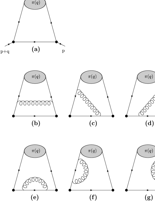
Figure 1: Feynman diagrams contributing to the correlation function (3): (a) zeroth order in $\alpha_{s}$, (b-g) first order in $\alpha_{s}$.

Figure 2: Light-cone sum rule estimate for $f_{B}f^{+}(0)$ in leading twist 2 approximation as a function of the Borel parameter $M^{2}$: NLO (solid ) in comparison to LO (dashed).

Figure 3: Momentum dependence of the form factor $f^{+}(p^{2})$ in leading twist 2 approximation: LO (dashed) in comparison to NLO (solid).

Figure 4: Scale dependence of the light-cone sum rule estimate of $f_{B}f^{+}(0)$ in leading twist 2 approximation: NLO (solid) in comparison to LO (dotted).

References

[1]
V.L. Chernyak and A.R. Zhitnitsky,
JETP Lett. 25 (1977) 510;
Sov. J. Nucl. Phys. 31 (1980) 544;
Phys. Rep. 112 (1984) 173.
[2]
A.V. Efremov and A.V. Radyushkin,
Phys. Lett. B94 (1980) 245;
Teor. Mat. Fiz. 42 (1980) 147.
[3]
G.P. Lepage and S.J. Brodsky,
Phys. Lett. B87 (1979) 359;
Phys. Rev. D22 (1980) 2157.
[4] V.M. Belyaev, A. Khodjamirian and R. Rückl,
Z. Phys. C 60 (1993) 349 .
[5] V.M. Belyaev, V.M. Braun,
A. Khodjamirian and R. Rückl,
Phys. Rev D 51 (1995) 6177.
[6]
A. Khodjamirian and R. Rückl, in “Continuous Advances in QCD 1996”,
edited
by M.I. Polikarpov ( World Scientific, Singapore, 1996), pp. 75-83;
A. Khodjamirian, R. Rückl and
Ch. Winhart , in preparation .
[7] F. del Aguila and M.K. Chase,
Nucl. Phys. B193 (1981) 517.
[8] E. Braaten, Phys. Rev. D28 (1983) 524.
[9] E.P. Kadantseva, S.V. Mikhailov and A.V. Radyushkin,
Sov. J. Nucl. Phys. 44 (1986) 326.
[10]
F.M. Dittes and A.V. Radyushkin, Phys. Lett. B134 (1984) 359;
M.H. Sarmadi, Phys. Lett. B143 (1984) 471;
S.V. Mikhailov and A.V. Radyushkin, Nucl. Phys. B254 (1985) 89.
[11] D.J. Broudhurst and S.C. Generalis, preprint
OUT-4102-8/R (1981) (unpublished);
D.J. Broadhurst, Phys. Lett. B101 (1981) 423;
T.M. Aliev and V.I. Eletsky, Sov. J. Nucl. Phys. 38 (1983) 936.
[12] Particle Data Group, Phys. Rev. D54 (1996) 1.
[13] V.M. Braun and I.E. Filyanov, Z. Phys. C48 (1990) 239.
[14]V.M. Braun and I.E. Filyanov, Z. Phys. C44 (1989) 157.
[15] A. Gonzales-Arroyo, C. Lopez and F.J. Yndurain,
Nucl. Phys. B153 (1979) 161.
[16] P. Ball, V.M. Braun and H.G. Dosch, Phys. Lett.
B273 (1991) 316.
[17] A. Szczepaniak, Phys. Rev. D54 (1996) 1167.