DTP/97/44

RAL TR 97-027

hep-ph/9706297

The One-loop QCD Corrections for $\gamma^{*}\to q\bar{q}gg$
J. M. Campbell, E. W. N.  Glover
Physics Department, University of Durham,
Durham DH1 3LE, England

and

D. J. Miller
Rutherford Appleton Laboratory, Chilton,
Didcot, Oxon, OX11 0QX, England

June 1997

We compute the one-loop QCD amplitudes for the decay of an off-shell vector boson with vector couplings into a quark-antiquark pair accompanied by two gluons keeping, for the first time, all orders in the number of colours. Together with previous work this completes the calculation of the necessary one-loop amplitudes needed for the calculation of the next-to-leading order ${\cal O}(\alpha_{s}^{3})$ corrections to four jet production in electron-positron annihilation, the production of a gauge boson accompanied by two jets in hadron-hadron collisions and three jet production in deep inelastic scattering.

Multi-jet events in electron-positron annihilation have long been a source of vital information about the structure of QCD. In 1979, three jet events at DESY gave the first clear indications of the existence of the gluon [1], while more recently, the colour factors that determine the gauge group of QCD have been determined [2]. While the general features of events have been well described by leading order predictions, many quantities are known to suffer large radiative corrections. For example, the experimental four jet rate measured as a function of the jet resolution parameter $y_{\rm cut}$, was significantly higher than the leading order expectation. This is of particular interest at LEP II energies where 4 jet events are the main background to $WW$ events where both $W$ bosons decay hadronically.

Recently there has been much progress towards a more complete theoretical description of four jet events produced in electron-positron annihilation. Dixon and Signer [3] have created a general purpose Monte Carlo program to evaluate the next-to-leading order corrections to a wide variety of four-jet and related observables. Such numerical programs have three important ingredients; the one-loop four parton amplitudes, the tree-level five parton amplitudes and a method for combining the four and five parton final states together. The tree-level amplitudes for $e^{+}e^{-}\to q\bar{q}ggg$ and $e^{+}e^{-}\to q\bar{q}Q\bar{Q}g$ are well known [4, 5, 6] and several general methods have been developed for numerically isolating the infrared divergences [7, 8, 9]. However, the one-loop amplitudes are not fully known, and the next-to-leading order corrections described by the Dixon-Signer program [3] are therefore incomplete.

The one-loop amplitudes relevant for this process are $e^{+}e^{-}\to q\bar{q}gg$ and $e^{+}e^{-}\to q\bar{q}Q\bar{Q}$. Two groups [10, 11] have computed the amplitudes for the four quark final states keeping all orders in the number of colours, and these matrix elements have been implemented in the Dixon-Signer Monte Carlo [3]. The situation for the two quark two gluon process is less complete and may be illustrated by examining the colour structure of the one-loop contribution to the four-jet cross section,

$$\sigma_{{\rm q\bar{q}gg}}^{{\rm 1-loop}}=N^{2}(N^{2}-1)\left(\sigma^{(a)}+\frac{1}{N^{2}}\sigma^{(b)}+\frac{1}{N^{4}}\sigma^{(c)}\right),$$ (1)

where $N$ is the number of colours. Bern, Dixon and Kosower [12] have provided compact analytic results for the leading colour part of the two quark two gluon process ($\sigma^{(a)}$) which should account for approximately 90% of the next-to-leading order corrections. Indeed, keeping all of the known contributions, Dixon and Signer find that the next-to-leading order predictions match onto the experimental data much better [3]. However, the subleading terms $\sigma^{(b)}$ and $\sigma^{(c)}$ are still expected to contribute a further 10% to the 4-jet rate. In this letter, we compute the one-loop matrix elements for the $\gamma^{*}\to q\bar{q}gg$ process keeping, for the first time, all orders in the number of colours. These results can be implemented directly into the Dixon-Signer Monte Carlo [3], or can be used as a cross check with the results anticipated from the helicity approach [13].

As in the calculation of the one-loop four quark matrix elements [10] and in contrast to the helicity method employed by Bern et al. [11], we compute ‘squared’ matrix elements, i.e. the interference between tree-level and one-loop amplitudes. By doing so, we reduce all tensor integrals down to scalars directly leaving at worst three (tensor) loop momenta in the numerator of the box integrals.

The evaluation of the tensor integrals represents the bulk of the calculation and should be treated with some care. The ‘squared’ tree-level matrix element for a given process contains inverse powers of certain invariants, resulting from the propagators present. This singularity structure is largely responsible for the infrared behaviour of the matrix elements. Based on general arguments, one expects that the one-loop corrections should have the same singularity structure as tree-level and should not contain more inverse powers of these (or other) invariants or additional kinematic singularities resulting from the calculational scheme used. However, as well as generating extra inverse powers of the invariants (above and beyond the expected tree-level singularities), traditional methods of reducing the tensor integrals to combinations of scalar integrals introduce (many) factors of the Gram determinant ($\Delta$) in the denominator. Although the matrix elements themselves are finite as $\Delta\to 0$, individual terms appear to diverge. These apparent singularities can be avoided by forming suitable combinations of the scalar integrals which are finite in the limit of vanishing $\Delta$ as well as in the limit where the invariant mass of a pair of particles tends to zero. Motivated by the work of Bern et al, [14], we have shown in ref. [15] how these functions are naturally obtained by differentiation of the original scalar loop-integral. The advantages of this decomposition are then two-fold. First, the expressions for the one-loop matrix elements are significantly simplified by grouping integrals together. Second, we can ensure that the one-loop singularity structure reproduces that at tree level. In other words, the only allowed kinematic singularities are those appearing at tree level, multiplied by coefficients that are well behaved in all kinematic limits. This latter point is achieved by using identities amongst the set of basic functions and tends not to reduce the size of the answer, although the absence of further kinematic singularities ensures that the matrix elements are numerically stable. There is a slight price to pay in that, compared to the raw scalar integrals, the the set of basic functions is now enlarged and is not linearly independent, resulting in some ambiguity in the form of the final result. To generate and simplify our results, we have made repeated use of the algebraic manipulation packages FORM and MAPLE.

For the process under consideration, $\gamma^{*}\to q\bar{q}gg$ we label the momenta as,

$$\gamma^{*}(p_{1234})\to q(p_{1})+\bar{q}(p_{2})+g(p_{3})+g(p_{4}),$$ (2)

and systematically eliminate the photon momentum in favour of the four massless parton momenta.

The colour structure of the matrix element at tree-level $(n=0)$ and one-loop $(n=1)$ is rather simple and we have,

$${\cal M}^{(n)}=\epsilon^{\mu}\epsilon^{\nu_{3}}\epsilon^{\nu_{4}}{\cal M}_{\mu\nu_{3}\nu_{4}}^{(n)}=eg_{s}^{2}\left(\frac{g_{s}}{4\pi}\right)^{2n}$$ (3)

$$\times \left\{(T^{a_{3}}T^{a_{4}})_{c_{1}c_{2}}{\cal A}^{(n)}_{1}(3,4)+(T^{a_{4}}T^{a_{3}})_{c_{1}c_{2}}{\cal A}^{(n)}_{1}(4,3)+\frac{1}{2}\delta_{c_{1}c_{2}}\delta_{a_{3}a_{4}}{\cal A}^{(n)}_{2}(3,4)\right\},$$

where $c_{1}$, $c_{2}$ are the colours of the quarks and $a_{3}$, $a_{4}$ the colours of the gluons. The arguments of ${\cal A}_{i}$ indicate a permutation of the momenta of the external gluons. At lowest order,

$${\cal A}^{(0)}_{2}(3,4)=0,$$ (4)

while at one-loop we find,

$${\cal A}^{(1)}_{1}(3,4) = N{\cal A}^{(1)}_{A}(3,4)-\frac{1}{N}{\cal A}^{(1)}_{B}(3,4),$$ (5)

$${\cal A}^{(1)}_{2}(3,4) \equiv {\cal A}^{(1)}_{C}(3,4)\equiv{\cal A}^{(1)}_{C}(4,3).$$ (6)

The functions $A^{(1)}_{\alpha}(i,j)$, $\alpha=A,B,C$ represent the contributions of the three gauge invariant sets of Feynman diagrams shown in Figs. 1, 2 and 3 respectively. We note that the contribution ${\cal A}^{(1)}_{A}(3,4)$ also includes terms proportional to $n_{F}/N$, where $n_{F}$ is the number of light quark flavours. These terms originate from the fermionic self-energy and triple gluon vertex corrections shown in the last two diagrams of Fig. 1. The Dixon-Signer Monte Carlo [3] incorporates the leading colour term, ${\cal A}^{(1)}_{A}(3,4)$.

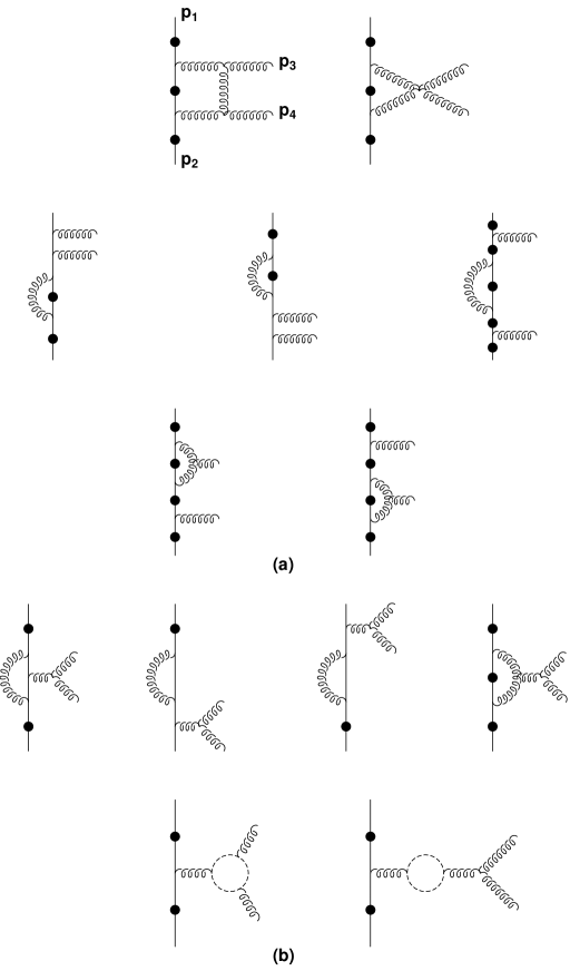
Figure 1: The classes of Feynman diagrams relevant for the function ${\cal A}^{(1)}_{A}(3,4)$. Reading clockwise round the diagram and starting from the quark ($p_{1}$) at the top, we encounter gluon ($p_{3}$) before gluon ($p_{4}$) and end at antiquark ($p_{2}$). The solid circle indicates the possible positions for attaching the off-shell photon to the quark-antiquark pair. Diagrams (a), taken with both permutations of gluons 3 and 4, contribute to the piece ${\cal L}_{A}$ while the permutation shown in (a)+(b) gives the contribution to ${\cal L}_{A}(3,4)$. Diagrams with self-energy corrections on the external lines are zero in dimensional regularisation and have been omitted.

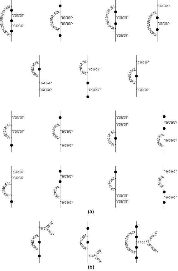
Figure 2: The classes of Feynman diagrams relevant for the function ${\cal A}^{(1)}_{B}(3,4)$ Reading clockwise round the diagram and starting from the quark ($p_{1}$) at the top, we encounter gluon ($p_{3}$) before gluon ($p_{4}$) and end at antiquark ($p_{2}$). The solid circle indicates the possible positions for attaching the off-shell photon to the quark-antiquark pair. Diagrams (a), taken with both permutations of gluons 3 and 4, contribute to the piece ${\cal L}_{B}$ while the permutation shown in (a)+(b) gives the contribution to ${\cal L}_{B}(3,4)$.

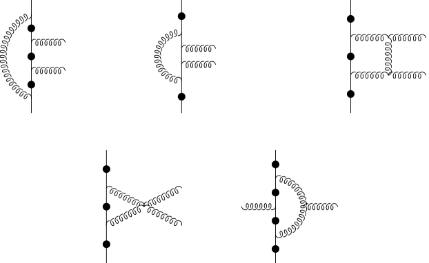
Figure 3: The classes of Feynman diagrams relevant for the function ${\cal A}^{(1)}_{C}$ when taken with both permutations of the gluons. Reading clockwise round the diagram and starting from the quark ($p_{1}$) at the top, we encounter gluon ($p_{3}$) before gluon ($p_{4}$) and end at antiquark ($p_{2}$). The solid circle indicates the possible positions for attaching the off-shell photon to the quark-antiquark pair.

The squared matrix elements are relatively straightforwardly obtained at leading order [16]. Some care must be taken to ensure that only physical, transverse degrees of freedom are included for the external gluons. We do this by requiring that terms in ${\cal M}_{\mu\nu_{3}\nu_{4}}^{(0)}$ that vanish when contracted with the physical gluon polarisation vectors $\epsilon^{\nu_{3}}$ or $\epsilon^{\nu_{4}}$ are removed by hand [17]. The sum over the polarisations of all the gauge bosons may then be performed in the Feynman gauge,

$$\sum_{\rm spins}\epsilon^{\mu}\epsilon^{*\nu}=-g^{\mu\nu}.$$ (7)

Hence,

$$\sum_{\rm spins}|{\cal M}^{(0)}|^{2}=\frac{e^{2}g_{s}^{4}}{4}(N^{2}-1)N\Biggl{\{}{\cal T}(3,4)+{\cal T}(4,3)-\frac{1}{N^{2}}{\cal T}\Biggr{\}},$$ (8)

where,

$${\cal T}(3,4)=\sum_{\rm spins}\Big{|}A_{1}^{(0)\dagger}(3,4){\cal A}_{1}^{(0)}(3,4)\Big{|},$$ (9)

and,

$${\cal T}=\sum_{\rm spins}\Big{|}\left(A_{1}^{(0)\dagger}(3,4)+A_{1}^{(0)\dagger}(4,3)\right)\left({\cal A}_{1}^{(0)}(3,4)+{\cal A}_{1}^{(0)}(4,3)\right)\Big{|}.$$ (10)

The 3-gluon vertex contributions to ${\cal A}_{1}^{(0)}(3,4)$ and ${\cal A}_{1}^{(0)}(4,3)$ enter with opposite sign, so ${\cal T}$ (with no arguments) is the contribution from the pure QED-like diagrams.

The relevant ‘squared’ matrix elements are the interference between the tree-level and one-loop amplitudes,

$$\sum_{\rm spins}2|{\cal M}^{(0)\dagger}{\cal M}^{(1)}|=\frac{e^{2}g_{s}^{4}}{4}\left(\frac{\alpha_{s}N}{2\pi}\right)(N^{2}-1)N$$ (11)

$$\times \Biggl{\{}{\cal L}_{A}(3,4)+{\cal L}_{A}(4,3)-\frac{1}{N^{2}}\biggl{(}{\cal L}_{A}+{\cal L}_{B}(3,4)+{\cal L}_{B}(4,3)-{\cal L}_{C}\biggr{)}+\frac{1}{N^{4}}{\cal L}_{B}\Biggr{\}},$$

with,

$${\cal L}_{\alpha}(3,4)=\sum_{\rm spins}\Big{|}A^{(1)\dagger}_{\alpha}(3,4){\cal A}_{1}^{(0)}(3,4)\Big{|},$$ (12)

for $\alpha=A,~{}B$ and the QED-like structures,

$${\cal L}_{\alpha}=\sum_{\rm spins}\Big{|}\left(A^{(1)\dagger}_{\alpha}(3,4)+A^{(1)\dagger}_{\alpha}(4,3)\right)\left({\cal A}_{1}^{(0)}(3,4)+{\cal A}_{1}^{(0)}(4,3)\right)\Big{|}.$$ (13)

Hence the ‘squared’ matrix elements are described by 5 independent ${\cal L}_{\alpha}$. The ${\cal L}_{\alpha}(3,4)$ are symmetric under the exchange $p_{1}\leftrightarrow p_{2}$ and $p_{3}\leftrightarrow p_{4}$ while the ${\cal L}_{\alpha}$ are symmetric under either $p_{1}\leftrightarrow p_{2}$ or $p_{3}\leftrightarrow p_{4}$.

Working in dimensional regularisation with $4-2\epsilon$ spacetime dimensions, it is straightforward to remove the infrared and ultraviolet poles from the ${\cal L}_{\alpha}$ since they are proportional to the tree-level amplitudes,

$${\cal L}_{A}(3,4) = \left(-\frac{{\cal P}_{13}}{\epsilon^{2}}-\frac{{\cal P}_{24}}{\epsilon^{2}}-\frac{{\cal P}_{34}}{\epsilon^{2}}-\frac{3}{2}\frac{{\cal P}_{1234}}{\epsilon}\right){\cal T}(3,4)+\hat{\cal L}_{A}(3,4),$$ (14)

$${\cal L}_{A} = +\frac{1}{2}\left(-\frac{{\cal P}_{13}}{\epsilon^{2}}-\frac{{\cal P}_{24}}{\epsilon^{2}}-\frac{{\cal P}_{34}}{\epsilon^{2}}-\frac{3}{2}\frac{{\cal P}_{1234}}{\epsilon}\right)\left({\cal T}+{\cal T}(3,4)-{\cal T}(4,3)\right)$$ (15)

$$+\frac{1}{2}\left(-\frac{{\cal P}_{14}}{\epsilon^{2}}-\frac{{\cal P}_{23}}{\epsilon^{2}}-\frac{{\cal P}_{34}}{\epsilon^{2}}-\frac{3}{2}\frac{{\cal P}_{1234}}{\epsilon}\right)\left({\cal T}+{\cal T}(4,3)-{\cal T}(3,4)\right)+\hat{\cal L}_{A},$$

$${\cal L}_{B}(3,4) = \left(-\frac{{\cal P}_{12}}{\epsilon^{2}}-\frac{3}{2}\frac{{\cal P}_{1234}}{\epsilon}\right){\cal T}(3,4)+\hat{\cal L}_{B}(3,4),$$ (16)

$${\cal L}_{B} = \left(-\frac{{\cal P}_{12}}{\epsilon^{2}}-\frac{3}{2}\frac{{\cal P}_{1234}}{\epsilon}\right){\cal T}+\hat{\cal L}_{B},$$ (17)

$${\cal L}_{C} = +\frac{1}{2}\left(-\frac{{\cal P}_{12}}{\epsilon^{2}}-\frac{{\cal P}_{34}}{\epsilon^{2}}+\frac{{\cal P}_{14}}{\epsilon^{2}}+\frac{{\cal P}_{23}}{\epsilon^{2}}\right)\left({\cal T}+{\cal T}(3,4)-{\cal T}(4,3)\right)$$ (18)

$$+\frac{1}{2}\left(-\frac{{\cal P}_{12}}{\epsilon^{2}}-\frac{{\cal P}_{34}}{\epsilon^{2}}+\frac{{\cal P}_{13}}{\epsilon^{2}}+\frac{{\cal P}_{24}}{\epsilon^{2}}\right)\left({\cal T}+{\cal T}(4,3)-{\cal T}(3,4)\right)+\hat{\cal L}_{C}.$$

where we have introduced the notation,

$${\cal P}_{x}=\left(\frac{4\pi\mu^{2}}{-s_{x}}\right)^{\epsilon}\frac{\Gamma^{2}(1-\epsilon)\Gamma(1+\epsilon)}{\Gamma(1-2\epsilon)}.$$ (19)

In physical cross sections, this pole structure cancels with the infrared poles from the $\gamma^{*}\to q\bar{q}gg+g$ process and those generated by ultraviolet renormalisation.

In determining the finite pieces, $\hat{\cal L}$, we are concerned to ensure that the singularity structure matches that of the tree-level functions ${\cal T}(3,4)$ and ${\cal T}$. In terms of the generalised Mandelstam invariants,

$$s_{ij}=(p_{i}+p_{j})^{2},\qquad s_{ijk}=(p_{i}+p_{j}+p_{k})^{2},\qquad s_{ijkl}=(p_{i}+p_{j}+p_{k}+p_{l})^{2},$$ (20)

${\cal T}$ contains single poles in $s_{13}$, $s_{23}$, $s_{14}$ and $s_{24}$ while ${\cal T}(3,4)$ has poles in $s_{13}$, $s_{34}$ and $s_{24}$. In addition, both ${\cal T}$ and ${\cal T}(3,4)$ contain double poles in the triple invariants $s_{134}$ and $s_{234}$. Using the tensor reduction described in [15], possible singularities due to Gram determinants are automatically protected. However, it is possible to generate apparent singularities in double or triple invariants such as $s_{12}$ or $s_{123}$. These poles do not correspond to any of the allowed infrared singularities and the matrix elements are finite as, for example, $s_{12}\to 0$ or $s_{123}\to 0$. In fact, it is straightforward to explicitly remove such poles using identities amongst the combinations of scalar integrals. For example, the identity,

$$\frac{(s_{123}-s_{12})}{s_{123}}{\rm Ld}_{22}(p_{12},p_{3},p_{4})=-{\rm Ld}_{21}(p_{12},p_{3},p_{4})+{\rm Ld}_{1}(p_{12},p_{3},p_{4})+{\rm Lc}_{1}(p_{12},p_{34}),$$ (21)

relating the functions for box integral functions with two adjacent masses (defined in Appendix B of [15]) is useful to eliminate poles in $s_{123}$. The finite pieces can be written symbolically as,

$$\hat{\cal L}=\sum_{i}P_{i}(s){\rm L}_{i},$$ (22)

where the coefficients $P_{i}(s)$ are rational polynomials of invariants. The finite functions ${\rm L}_{i}$ are the linear combinations of scalar integrals defined in [15] which are well-behaved in all kinematic limits. Any denominators of the corresponding tree-level matrix element are allowed in the coefficient $P_{i}(s)$, with any additional fake singularities protected by ${\rm L}_{i}$. Typically the coefficient of a given function contains ${\cal O}(100)$ terms, comparable with the size of the tree-level matrix elements. The number of functions is rather large, of ${\cal O}(100)$, but is a minimal set which protects all the kinematic limits and is therefore numerically stable. The analytic expressions for the individual $\hat{\cal L}_{\alpha}$, and particularly the subleading colour terms $\hat{\cal L}_{B}$ and $\hat{\cal L}_{C}$, are therefore rather lengthy so we have constructed a FORTRAN subroutine to evaluate them for a given phase space point. This can be directly implemented in general purpose next-to-leading order Monte Carlo programs for the $e^{+}e^{-}\to 4~{}{\rm jet}$, $e^{\pm}p\to e^{\pm}+3~{}{\rm jet}$ and $p\bar{p}\to V+2~{}{\rm jet}$ processes.

To summarize, we have performed the first calculation of the one-loop ‘squared’ matrix elements for the $\gamma^{*}\to q\bar{q}gg$ process keeping all orders in the number of colours. We have grouped the Feynman diagrams according to the colour structure, but unlike the helicity approach of [18], have used conventional dimensional regularisation throughout. We have used the one-loop reduction method described in [15] to obtain the finite parts of the one-loop matrix amplitudes in terms of functions that are well behaved in all kinematic limits. The finite one-loop expressions $\hat{\cal L}_{\alpha}$ contain the same singularity structure as the tree level amplitudes ${\cal T}$ and are numerically stable. Our results are rather lengthy and we have provided a FORTRAN implementation of them that can be either used with the existing Dixon-Signer program for $e^{+}e^{-}\to 4$ jets or as a completely independent check of amplitudes obtained using the helicity approach [11, 12, 13]. Together with previous work [10, 11, 12] this completes the calculation of the necessary one-loop amplitudes for the coupling of an electroweak gauge boson to four massless partons with the following exceptions:

• Contributions proportional to the axial coupling.

• Contributions where the electroweak boson couples to a closed fermion loop.

Both of these contributions are expected to be small because of cancellations between the up- and down-type quark contributions.

Acknowledgements

We thank Walter Giele, Eran Yehudai, Bas Tausk and Keith Ellis for collaboration in the earlier stages of this work. JMC thanks the UK Particle Physics and Astronomy Research Council for the award of a research studentship.

References

- [1] See for example, P. Söding, B. Wiik, G. Wolf and S. L. Wu, Proc. Int. Europhysics Conf. on High Energy Physics, Brussels August 1995, (World Scientific, Singapore, 1995), p.3.
-
[2]
B. Adeva et al, L3 Collaboration, Phys. Lett. B248 (1990) 227;
P. Abreu et al, DELPHI Collaboration, Z. Phys. C59 (1993) 357;
R. Akers et al, OPAL Collaboration, Z. Phys. C65 (1995) 367;
R. Barate et al, ALEPH Colaboration, CERN preprint CERN-PPE/97-002. -
[3]
L. Dixon and A. Signer,
Phys. Rev. Lett. 78 (1997) 811;
A. Signer, ‘Next-to-Leading Order Corrections to Four Jets’, hep-ph/9705218. - [4] K. Hagiwara and D. Zeppenfeld, Nucl. Phys. B313 (1989) 560.
- [5] F. A. Berends, W. T. Giele and H. Kuijf, Nucl. Phys. B321 (1989) 39.
- [6] N. K. Falk, D. Graudenz and G. Kramer, Nucl. Phys. B328 (1989) 317.
-
[7]
K. Fabricius, I. Schmitt, G. Kramer and G. Schierholz,
Z. Phys. C11 (1981) 315;
W. T. Giele and E. W. N. Glover, Phys. Rev. D46 (1992) 1980. -
[8]
R. K. Ellis, D. A. Ross and A. E. Terrano, Nucl. Phys. B178 (1981)
421;
S. Frixione, Z. Kunszt and A. Signer, Nucl. Phys. B467 (1996) 399;
S. Catani and M.H. Seymour, Nucl. Phys. B485 (1997) 291. - [9] E. W. N. Glover and M. R. Sutton, Phys. Lett. B342 (1995) 375.
- [10] E. W. N. Glover and D. J. Miller, Phys. Lett. B396 (1997) 257.
- [11] Z. Bern, L. Dixon, D. A. Kosower and S. Wienzierl, Nucl. Phys. B489 (1997) 3.
- [12] Z. Bern, L. Dixon and D. A. Kosower, Nucl. Phys. Proc. Suppl. 51C (1996) 243.
- [13] Z. Bern, L. Dixon and D. A. Kosower, in preparation.
- [14] Z. Bern, L. Dixon and D. A. Kosower, Nucl. Phys. B412 (1994) 751.
- [15] J. M. Campbell, E. W. N. Glover and D. J. Miller, ‘One-Loop Tensor Integrals in Dimensional Regularisation’, hep-ph/9612413, to appear in Nucl. Phys. B.
- [16] R. K. Ellis, D. A. Ross and A. E. Terrano, Nucl. Phys. B178 (1981) 421.
-
[17]
H. M. Georgi et al, Annals of Physics 114 (1978) 273;
B. L. Combridge, Nucl. Phys. B151 (1979) 429. - [18] see for example, Z. Bern, L. Dixon and D. A. Kosower, Ann. Rev. Nucl. Part. Sci. 46 (1996) 109.