BROWN-HET-1082 June 6, 1997

Diffractive Production at Collider Energies

I: Soft Diffraction and Dino’s Paradox

Chung-I Tan⁽¹⁾

⁽¹⁾Department of Physics, Brown University, Providence, RI 02912, USA

1 Introduction

One of the more interesting developments from recent collider experiments is the finding that hadronic total cross sections as well as elastic cross sections in the near-forward limit can be described by the exchange of a “soft Pomeron” pole, [1] i.e., the absorptive part of the elastic amplitudes can be approximated by ${Im}\>T_{a,b}(s,t)\simeq\beta_{a}(t)s^{\alpha_{\cal P}(t)}\beta_{b}(t).$ The Pomeron trajectory has two important features. [2] First, its zero-energy intercept is greater than one, $\alpha_{\cal P}(0)\equiv 1+\epsilon$, $\epsilon\simeq 0.08\sim 0.12$, leading to rising $\sigma^{tot}(s)$. Second, its Regge slope is approximately $\alpha_{\cal P}^{\prime}\simeq 0.25\sim 0.3$ $GeV^{-2}$, leading to the observed shrinkage effect for elastic peaks. The most important consequence of Pomeron being a pole is factorization. For a singly diffractive dissociation process, factorization leads to a “classical triple-Pomeron” formula, [4]

$${d\sigma\over dtd\xi}\rightarrow{d\sigma^{classical}\over dtd\xi}\equiv F_{{\cal P}/a}^{cl}(\xi,t)\sigma_{{\cal P}b}^{cl}(M^{2},t),$$ (1)

where $M^{2}$ is the missing mass variable and $\xi\equiv M^{2}/s$. The first term on the right-hand side of Eq. (1) is the so-called “Pomeron flux”, and the second term is the “Pomeron-particle” total cross section. Eq. (1) is in principle valid only when $\xi^{-1}$ and $M^{2}$ are both large, with $t$ small and held fixed. However, with $\epsilon\sim 0.1$, it has been observed [5] that the extrapolated $p\bar{p}$ single diffraction dissociation cross section, $\sigma^{sd}$, based on the standard triple-Pomeron formula is too large at Tevatron energies by as much as a factor of $5\sim 10$ and it could become larger than the total cross section.

Let us denote the singly diffractive cross section as a product of a “renormalization” factor and the classical formula,

$${d\sigma\over dtd\xi}=Z(\xi,t;s){d\sigma^{classical}\over dtd\xi}.$$ (2)

It was argued by K. Goulianos in Ref. [5] that agreement with data could be achieved by having an energy-dependent suppression factor, $Z(\xi,t;s)\rightarrow Z_{G}(s)\equiv N(s)^{-1}\leq 1$. This “renormalization” factor is chosen so that the new “Pomeron flux”, $F_{N}(s,\xi,t)\equiv N(s)^{-1}F_{{\cal P}/p}^{cl}(\xi,t)$, is normalized to unity for $s\geq\bar{s}$, $\sqrt{\bar{s}}\simeq 22\>GeV$. [5][6][7] However, the modified triple-Pomeron formula no longer has a factorized form. An alternative suggestion has been made recently by P. Schlein. [8][9] It was argued that phenomenologically, after incorporating lower triple-Regge contributions, the renomalization factor for the triple-Pomeron contribution could be described by an $\xi$-dependent suppression factor, $Z\rightarrow Z_{S}(\xi)$.

In view of the factorization property for total and elastic cross sections, the “flux renormalization” procedure appears paradoxical and could undermine the theoretical foundation of a soft Pomeron as a Regge pole from a non-perturbative QCD perspective. We shall refer to this as “Dino’s paradox”. Finding a resolution that is consistent with Pomeron pole dominance for elastic and total cross sections at Tevatron energies will be the main focus of this study. In particular, we want to maintain the following factorization property,

$${d\sigma\over dtd\xi}\rightarrow\sum_{k}D_{k}(\xi,t)\Sigma_{k}(M^{2}),$$ (3)

when $\xi^{-1}$ and $M^{2}$ become large. [11] It is our intention to provide a solution without deviating from generally accepted guiding principles for hadron dynamics.

It is reasonable to expect that the resolution to the paradox should lie in a proper implementation of screening corrections to the classical triple-Pomeron formula. One of our key observations is the fact that, since $\sigma^{sd}$ is approximately $15\%$ of the total cross section at Tevatron, a pole dominance picture for $\sigma^{tot}$ should also impose a direct constraint on the nature of diffractive production. The second observation is the necessity in having an overall coherent scheme in which various different hadronic energy scales must enter consistently. In our usage of classical triple-Regge formulas, the basic energy scale is always in terms of ${s_{0}}\simeq 1$ $GeV^{2}$. We demonstrate that there are at least two other energy scales, $s_{r}\equiv e^{y_{r}}$ and $s_{f}\equiv e^{y_{f}}$, $y_{r}\simeq 3\sim 5$ and $y_{f}\simeq 8\sim 10$, which must be incorporated properly. The first is associated with the physics of light quarks and the scale of chiral symmetry breaking. The second is the “flavoring” scale and is associated with “heavy flavor” production. In a non-perturbative QCD setting, both play an important role in our understanding of a bare Pomeron with an intercept greater than unity. [12][13]

Our treatment lies in a proper implementation of final-state screening correction, (or final-state unitarization), with “flavoring” for Pomeron as the primary dynamical mechanism for setting the relevant energy scale. In our treatment, initial-state screening remains unimportant, consistent with the pole dominance picture for elastic and total cross section hypothesis at Tevatron energies. The factor $D_{a,{\cal P}}(\xi,t)$ from the Pomeron contribution will be referred to as a “unitarized Pomeron flux factor,” and we shall occassionally refer to our procedure as “unitarization of Pomeron flux”. We shall demonstrate that in our unitarization scheme the total renormalization factor has a factorized form,

$$Z(\xi,t;s)=Z_{d}(\xi,t)Z_{m}(M^{2})=[S_{f}(\xi,t)R^{2}(\xi^{-1})]R(M^{2}),$$ (4)

where $S_{f}$ is due to final-state screening, Eq. (38). $R$ is a flavoring factor, given by Eq. (31), and there is one flavoring factor for each Pomeron propagator.

With the pole dominance hypothesis, we demonstrate that the unitarized flux factor, $D_{a,{\cal P}}(\xi,t)\equiv Z_{d}(\xi,t)F^{cl}_{a,{\cal P}}(\xi,t)$, must satisfy a normalization condition.

$$\int_{-\infty}^{0}dt\int_{0}^{1}{d\xi}D_{a,{\cal P}}(\xi,t)\xi^{\epsilon}\equiv\beta_{a}^{diff}<\beta_{a}(0).$$ (5)

The required damping to overcome the $\xi^{-(1+2\epsilon)}$ divergent behavior of $F^{cl}_{a,{\cal P}}(\xi,0)$ at small $\xi$ comes from both the screening factor $S_{f}(\xi,t)$ and the factor $\xi^{\epsilon}$ from the “Pomeron-particle” total cross section. More importantly, we point out that, even without screening, flavoring alone would lead to a suppression for the large $\xi^{-1}$ and large $M^{2}$ region at Tevatron energies of the order $\{{R(\infty)/R(1)}\}^{3}\simeq e^{-3\epsilon y_{f}}\simeq{1/8}$, where $R(\infty)=1$. For instance, flavoring leads to a suppression for the triple-Pomeron coupling

$$g_{\cal PPP}(0)\sim e^{-3\epsilon y_{f}/2}g^{low}_{\cal PPP}(0),$$ (6)

where $g^{low}_{\cal PPP}(0)\simeq 0.364\pm 0.025\>mb^{1\over 2}$ is that obtained in a fit to low-energy data. [14] In other words, the apparent unitarity violation will be mostly alleviated by flavoring alone! Lastly we emphasize, since factorization remains intact, our unitarization scheme leads to unambiguous predictions in terms of these suppression factors for double Pomeron exchange, doubly diffraction dissociation, etc., both at Tevatron and at LHC energies.

In Section II, we explain why, given the Pomeron pole dominance hypothesis, the initial-state screening cannot be large at Tevatron energies. We introduce the notion of “rapidity gap” cross sections and explain the sum rule, Eq. (5). We study in Sec. III the effect of final-state absorption. In particular, we demonstrate that, with Pomeron intercept greater than one, absorption is “total” within the “expanding hadronic disk” and the residual inelastic scattering can only take place on the “edge” of the disk. It follows that unitarity will not be violated by diffraction dissociation within a pole dominance picture for $\sigma^{tot}$. A model for calculating the screening factor, $S_{f}(\xi,t)$, is introduced. In Sec. IV we discuss the origin of the flavoring energy scale and indicate its relevant for diffractive dissocition cross sections. In a scale-dependent formulation, we explain how flavoring contributes factors $R^{2}(\xi^{-1})$ and $R(M^{2})$ to $Z(\xi,t;s)$ in order to account for both the Pomeron pole and coupling renormalizations. The flavoring function $R$ can be expressed in terms of a scale-dependent “effective” Pomeron intercept, $\epsilon_{eff}(y)$.

Putting these together, we provide the final recipe for our resolution to Dino’s paradox in Sec. V. Phenomenologically simple parametrizations for both the screening function, $S_{f}$, and the effective intercept, $\epsilon_{eff}$, are presented. Readers interested only in our proposed modification to the classical triple-Pomeron formula can go there directly. We present a phenomenological analysis which yields an estimate for the “high energy” triple-Pomeron coupling:

$$g_{\cal PPP}(0)\simeq.14\sim.20\>\>{mb}^{{\textstyle{1\over 2}}}.$$ (7)

This value is consistent with our flavoring expectation, Eq. (6). Surprisingly, the amount of screening required at Tevatron energies seems to be very small. We discuss our predictions for double Pomeron exchange, double diffraction dissociation, and other multi-gap processes in Sec. VI. Comparison of our approach to that of Refs. [5] and [8] as well as other comments are given in Sec. VII.

2 Pomeron Dominance Hypothesis at Tevatron Energies

We shall first explore consequences of the observation that both total cross sections and elastic cross sections can be well described by a Pomeron pole exchange at Tevatron energies. Absorption correction, if required, seems to remain small. Since the singly diffractive cross section, $\sigma^{sd}$, is a sizable part of the total, it must also grow as $s^{\epsilon}$. This qualitative understanding can be quantified in terms of a sum rule for “rapidity gap” cross sections. This in turn imposes a convergence condition on our unitarized Pomeron flux, $D_{a,{\cal P}}(\xi,t)$.

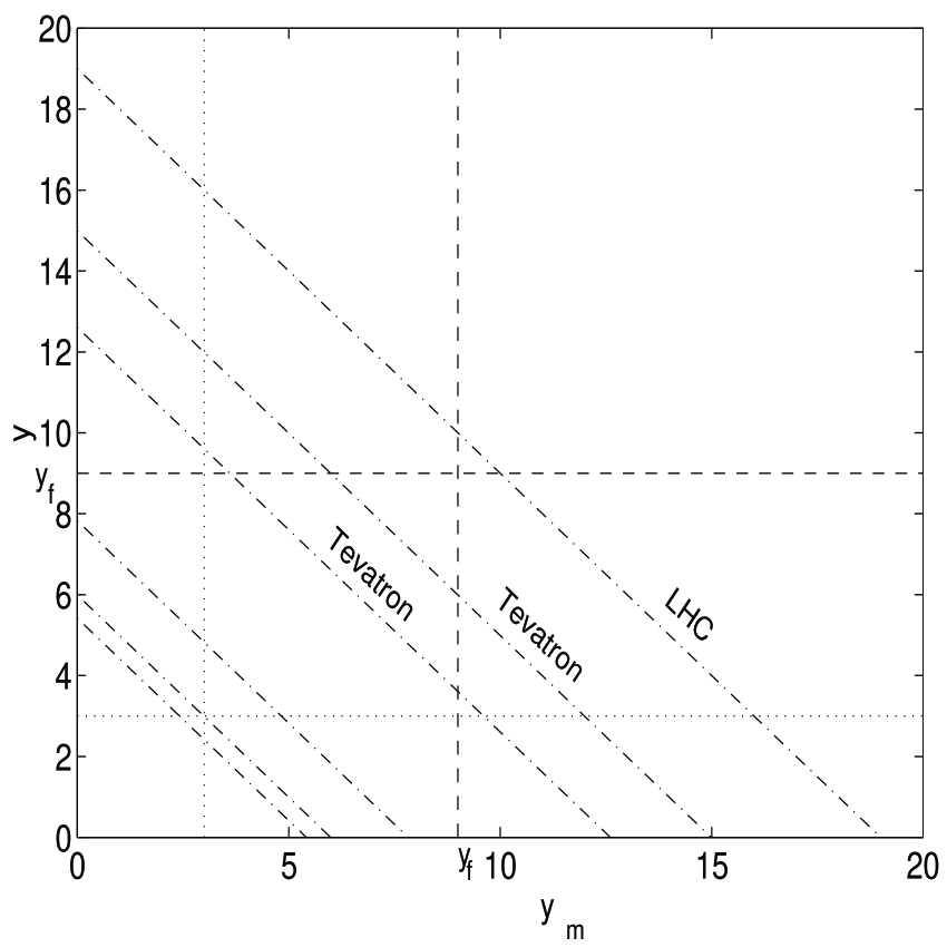
Figure 1: Phase space for single diffraction dissociation from ISR to LHC in terms of rapidity variables $y\equiv\log{\xi^{-1}}$ and $y_{m}\equiv\log M^{2}$. The dashed lines are for “flavoring” scale, $y_{f}$, chosen to be 9 for illustration. Dotted lines are $y_{min}\simeq 3$ lines for both $y$ and $y_{m}$. The Dashed-dotted lines are constant center of mass energy lines for $E_{i}$, $i=1,\cdots\cdots,6,$ equals to $15,30,60,546,1800,14,000\>GeV$ respectively.

To simplify the discussion, we shall first ignore transverse momentum distribution by treating the longitudinal phase space only. For instance, for singly diffraction dissociation, the longitudinal phase space can be specified by two rapidities, $y\equiv\log(\xi^{-1})$ and $y_{m}\equiv\log M^{2}.$ The first variable specifies the rapidity gap associated with the detected leading proton (or antiproton), and the second variable specifies the rapidity “span” of the missing mass distribution. At fixed $s$, they are constrained by $y+y_{m}\simeq Y\equiv\log s$, (see Figure 1), and we can speak of differential diffractive cross section $d\sigma^{sd}/dy$. We shall in what follows use $\{\xi^{-1},\>M^{2}\}$ and $\{y\equiv\log{\xi^{-1}},\>y_{m}\equiv\log M^{2}\}$ interchangably. Dependence on transverse degrees of freedom can be re-introduced without much effort after completing the main discussion.

Consider the process $a+b\rightarrow c+X^{<}$, where the number of particles in $X$ is unspecified. However, unlike the usual single-particle inclusive process, the superscript for $X^{<}$ indicates that all particles in $X$ must have rapidity less than that of the particle $c$, i.e., the detected particle $c$ is the one in the final state with the largest rapidity value. Kinematically, a single-gap cross section is identical to the singly diffraction dissociation cross section discussed earlier. Under the assumption where all transverse motions are unimportant, one has $y_{c}\simeq y_{a}\equiv Y_{max}$ and the differential gap cross section, ${d\sigma^{gap}/dy}$, can also be considered as a function of $y$ and $y_{m}$, with $y+y_{m}\simeq Y$.

Because the detected particle $c$ has been singled out to be different from all other particles, this is no longer an inclusive cross section, and it does not satisfy the usual inclusive sum rules. Upon integrating over the rapidity gap $y$ and summing over particle type $c$, no multiplicity enhancement factor is introduced and one obtains simply the total cross section, i.e., a gap cross section satisfies the following exact sum rule,

$$\sum_{c}\int dy{d\sigma_{ab\rightarrow c}^{gap}\over dy}\equiv\sum_{c}\sigma_{ab\rightarrow c}^{gap}=\sum_{n=2}^{\infty}\sigma_{n}=\sigma^{tot}_{ab}.$$ (8)

Interestingly, this allows an identification of the toal cross section as a sum over specific gap cross sections, $\sigma_{ab\rightarrow c}^{gap}$, each is “derived” from a specific “leading particle” gap distribution. Since no restriction has been imposed on the nature of the “gap distribution”, e.g., particle $c$ can have different quantum numbers from $a$, the notion of a gap cross section is more general than a diffraction cross section.[15] It follows that the singly diffractive dissociation cross section, $\sigma^{sd}_{ab}$, is a part of $\sigma_{ab\rightarrow a}^{gap}$.

Consider next our factorized ansatz, Eq. (3). For $y$ and $y_{m}$ large, it leads to a gap distribution, ${d\sigma_{ab\rightarrow c}^{gap}/dy}=e^{-y}D_{a\rightarrow c}(y)\Sigma_{b}(y_{m}).$ If $\Sigma_{b}(y_{m})=\beta_{b}e^{\epsilon y_{m}}$, it follows that contribution from each gap distribution is Regge behaved, $\sigma^{gap}_{ab\rightarrow c}\simeq\beta_{a}^{c}e^{\epsilon Y}\beta_{b}$, where the total Pomeron residue is a sum of “partial residues”,

$$\beta_{a}=\sum_{c}\beta_{a}^{c}=\sum_{c}\int_{0}^{\infty}dyD_{a}^{c}(y)e^{-\epsilon y},$$ (9)

For above integral to converge, each flux factor must grow slower than $e^{\epsilon y}$. That is, $D_{a}^{c}(y)e^{-\epsilon y}\rightarrow 0$ as $y\rightarrow\infty.$ In a traditional Regge approach, the large rapidity gap behavior for each flux factor is controlled by an approriate Regge propagator, $e^{(\alpha_{i}+\alpha_{j}-1)y}$. Clearly a standard triple-Pomeron behavior with $\alpha_{\cal P}>1$ is inconsistent with the pole dominance hypothesis. Unitarity correction must supply enough damping to provide convergence.

There is yet another way of expressing the consequence of the pole dominance hypothesis. Dividing each gap differential cross section by the total cross section, factorization of Pomeron leads to a “limiting distribution”: $\rho_{ab}(y,Y)\rightarrow\rho_{a}(y)\equiv\sum_{c}\rho_{a}^{c}(y).$ That is, the limit is independent of the total rapidity, $Y$, and the gap density is normalizable, $\int_{0}^{\infty}dy\rho_{a}(y)=\sum_{c}\int_{0}^{\infty}dy\rho_{a}^{c}(y)=\sum_{c}{(\beta_{a}^{c}/\beta_{a})}=1$. This normalization condition for the gap distribution is precisely Eq. (9).

Let us now restore the transverse distribution and concentrate on the diffractive dissociation contribution, which can be identified with the high $M^{2}$ and high $\xi^{-1}$ limit of $d\sigma^{gap}_{ab\rightarrow a}(t,\xi;M^{2})$. In terms of $\xi$, $M^{2}$, and $t$, the differential cross section at large $M^{2}$ under our factorizable ansatz takes on the following form, ${d\sigma_{ab}^{sd}/dtd\xi}\simeq D_{a,{\cal P}}(\xi,t)\Sigma^{cl}_{{\cal P},b}(M^{2}),$ where $\Sigma^{cl}_{{\cal P},b}(M^{2})=(M^{2})^{\epsilon}\beta_{b}(0).$ It follows from Eq. (9) that $D_{a,{\cal P}}(\xi,t)$ must satisfy the following bound:

$$\int_{-\infty}^{0}dt\int_{\xi_{min}(s)}^{\xi_{max}}{d\xi}D_{a,{\cal P}}(\xi,t)\xi^{\epsilon}\leq\int_{-\infty}^{0}dt\int_{0}^{1}{d\xi}D_{a,{\cal P}}(\xi,t)\xi^{\epsilon}\equiv\beta_{a}^{diff}<\beta_{a}(0).$$ (10)

The hypothesis of a Pomeron pole dominance for the total and elastic cross sections is of course only approximate. However, to the extend that absorptive corrections remain small at Tevatron energies, one finds that a modified Pomeron flux factor must differ from the “classical” Pomeron flux at small $\xi$ in such a way so that the upper bound in Eq. (10) is satisfied. We shall refer to $D_{a,{\cal P}}(\xi,t)$ as the “unitarized Pomeron flux”. How this can be accomplished via final state screening will be discussed next. Note both the similarity and the difference between Eq. (10) and the “flux normalization” condition mentioned in the Introduction. Here, this convergent integral yields a finite number, $\beta^{diff}_{a}$, and the ratio $\beta^{diff}_{a}/\beta_{a}(0)$ can be interpreted as the probability of having a diffractive gap at high energies.

3 Final-State Screening

The best known example for implementing the idea of “screening” in high energy hadronic collisions has been the “expanding disk” picture for rising total cross sections. Diffraction scattering as the shadow of inelastic production has been a well established mechanism for the occurence of a forward peak. Analyses of data upto collider energies have revealed that the essential feature of nondiffractive particle production can be understood in terms of a multipertipheral cluster-production mechanism. In such a picture, the forward amplitude is predominantly absorptive and is dominated by the exchange of a “bare Pomeron”. If the Pomeron intercept is greater than one, it forces further unitarity corrections as one moves to higher energies. For instance, saturation of the Froiossart bound can be next understood through an eikonel mechanism, with the absorptive eikonal $\chi(s,b)$ given by the bare Pomeron amplitude in the impact-parameter space.

The main problem we are facing here is not so much on how to obtain a “most accuraate” flux factor $D_{a,{\cal P}}(\xi,t)$ at very small $\xi$. We are concerned with a more difficult conceptual problem of how to reconcile having a potentially large screening effect for diffraction dissociation processes and yet being able to maintain approximate pole dominance for elastic and total cross sections up to Tevatron energies. We shall show using an expanding disk picture that absorption works in such a way that inelastic scattering can only take place on the “edge” of disk. [16] Therefore, once applied using final-state screening, the effect of initial-state absorption will be small, hence allowing us to maintain Pomeron pole factorization for elastic and total cross sections.

3.1 Expanding Disk Picture

Let us briefly review this picture which also serves to establish notations. At high energies, a near-forward amplitude can be expressed in an impact-parameter representaion via a two-dimensional Fourier transform,

$$T(s,t)\equiv 2is\int d^{2}{\vec{b}}e^{i\vec{q}\cdot\vec{b}}\tilde{f}(s,b),\hskip 30.0pt\tilde{f}(s,b)=(4i\pi s)^{-1}\int d^{2}\vec{q}e^{-i\vec{b}\cdot\vec{q}}T(s,t),$$ (11)

where $t\simeq-\vec{q}^{2}$. Assume that the near-forward elastic amplitude at moderate energies can be described by a Born term, e.g., that given by a single Pomeron exchange where we shall approximate it to be purely absorptive. Let us denote the contribution from the Pomeron exchange to $\tilde{f}(s,b)$ as $\chi(s,b)$. With $\alpha_{\cal P}(t)=1+\epsilon+\alpha^{\prime}_{\cal P}t$, and approximating $\beta(t)$ by an exponential, we find $\chi(s,b)\simeq X(s)e^{-(b^{2}/4B(s))}$,

$$X(s)\equiv\chi(s,0)\simeq{\sigma_{0}(s)\over 4B(s)}$$ (12)

where $B(s)=b_{0}+\alpha^{\prime}_{\cal P}\log s$ and $\sigma_{0}(s)=\sigma_{0}s^{\epsilon}$. With $\epsilon>0$, the Born approximation would eventually violate $s$-channel unitarity at small $b$ as $s$ increases. A systematic procedure which in principle should restore unitarity is the Reggeon calculus. However, our current understanding of dispersion-unitarity-relation is too qualitative to provide a definitive calculational scheme.

The key ingredient of “screening” correction is the recognition that the next order correction to the Born term must have a negative sign. (The sign of double-Pomeron cut contribution.) In an impact-representation, Reggeon calculus assures us that the correction can be represented as

$$\tilde{f}_{1}(s,b)\simeq-{1\over 2!}\>\mu(s)\>\chi(s,b)^{2},$$ (13)

where $\mu$ is positive. To go beyond this, one needs a model. A physically well-motivated model which should be meaningful at moderate energies and allows easy analytic treatment is the eikonal model. Writing $\tilde{f}(s,b)=\tilde{f}_{0}(s,b)+\tilde{f}_{1}(s,b)+\tilde{f}_{2}(s,b)+\cdots,$ the expansion alternates in sign, and with simple weights such that $\tilde{f}(s,b)=[1-e^{-\mu\chi(s,b)}]/\mu$, and

$$T(s,t)=({2is\over\mu})\int d^{2}{\vec{b}}\>e^{i\vec{q}\cdot\vec{b}}\{1-e^{-\mu\chi(s,b)}\}.$$ (14)

Conventional eikonal model has $\mu=1$. We keep $\mu\leq 1$ here so as to allow the possibility that screening is “imperfect”.

Observe that the eikonal derived from the Pomeron exchange, $\chi(s,b)$, is a monotonically decreasing function of $b^{2}$, taking on its maximum value $X(s)$ at $b^{2}=0$, which increases with $s$ due to $\epsilon>0$. The eikonal drops to zero at large $b^{2}$ and is of the order $1$ at a radius, $b_{c}(s)\simeq\sqrt{B(s)\log\mu X(s)}\sim\log s.$ Within this radius, $\tilde{f}(s,b)=O(1)$ and it vanishes beyond. This is the “expansion disk” picture of high energy scattering, leading to an asymptotic total cross section $O(b_{c}(s)^{2})$.

3.2 Inelastic Screening

In order to discuss inelastic final-state screening, we follow the “shadow” scattering picture in which the “minimum biased” events are predominantly “short-range ordered” in rapidity and the production amplitudes can be described by a multiperipheral cluster model. Substituting these into the right-hand side of an elastic unitary equation, $ImT(s,0)=\sum_{n}|T_{2,n}|^{2}$, one finds that the resulting elastic amplitude is dominated by the exchange of a Regge pole, which we shall provisionally refer to as the “bare Pomeron”. Next consider singly diffractive events. We assume that the “missing mass” component corresponds to no gap events, thus the distribution is again represented by a “bare Pomeron”. However, for the gap distribution, one would insert the “bare Pomeron” just generated into a production amplitude, thus leading to the classical triple-Pomeron formula.

Extension of this scheme leads to a “perturbative” treatment for the total cross section in the number of bare Pomeron exchanges along a multiperipheral chain. Such a scheme was proposed long time ago, [18] with the understanding that the picture could make sense at moderate energies, provided that the the intercept of the Pomeron is one, $\alpha(0)\simeq 1$, or less. However, with the acceptance of a Pomeron having an intercept greater than unity, this expansion must be embellished. Although it is still meaningful to have a gap expansion, one must improve the descriptions for parts of a production amplitude involving large rapidity gaps by taking into account absorptions for the gap distribution. We propose that this “partial unitarization” be done for each gap separately, thus maintaining the factorization property along each short-range ordered sector. This involves final-state screening, and, for singly diffraction dissociation, it corresponds to the inclusion of “enhanced Pomeron diagrams” in the triple-Regge region.

To simplify the notation, we shall use the energy variable, $\xi^{-1}$, and the rapidity gap variable, $y=\log(\xi^{-1})$, interchangeably. Let’s express the total unitarized contribution to a gap cross section in terms of a “unitarized flux” factor, $D(y,t)\equiv(e^{y}/16\pi)|g_{d}(y,t)|^{2}\equiv(1/16\pi\xi)|f_{d}(\xi,t)|^{2}{g_{\cal PPP}(t)},$ so that it reduces to the classical triple-Pomeron formula as its Born term. That is, the corresponding Born amplitude for $f_{d}(\xi,t)$ is the “square-root” of the triple-Pomeron contribution to the classical formula, $f^{cl}_{\cal P}(\xi,t)=\beta_{\cal P}(t)(\xi^{-1})^{(\alpha_{\cal P}(t)-1)}.$ Screening becomes important if large gap becomes favored, i.e., when $\epsilon>0$.

Let us work in an impact representation, $g(y_{d},t)\equiv{2i}\int d^{2}\vec{q}e^{i\vec{b}\cdot\vec{q}}\tilde{g}_{d}(y_{d},b).$ Consider an expansion $\tilde{g}(y,b)=\chi_{d}(y,b)+\tilde{g}_{1}(y,b)+\tilde{g}_{2}(y,b)+\cdots$ where, under the usual exponential approximation for the $t$-dependence, the Fourier transform for the Born term is $\chi_{d}(y,b)={\sigma^{d}(y)\over 4B_{d}(y)}e^{-{b^{2}\over 4B_{d}(y)}}$, with $B_{d}(y)=b_{d}+\alpha^{\prime}_{\cal P}y$ and $\sigma^{d}(y)=\sigma_{d}e^{\epsilon\>y}$. The key physics of absorption is

$$\tilde{g}_{1}(y,b)\simeq-\mu_{d}\chi(y,b)\chi_{d}(y,b).$$ (15)

The proportionality constant $\mu_{d}$ can be different from the constant $\mu$ introduced earlier for the elastic screening, either for kinematic or dynamic reasons, or both. For a generalized eikonal approximation, one has $\tilde{g}(y,b)=\chi_{d}\{1-\mu_{d}\chi+{1\over 2!}(\mu_{d}\chi)^{2}-\cdots\}=\chi_{d}(y,b)e^{\>-\mu_{d}\>\chi(y,b)}.$ If we define the “final-state screening” factor as the ratio between the unitarized flux factor and the classical triple-Pomeron formula, $D_{a,{\cal P}}(y,t)=S^{(0)}_{f}(y,t;X)F^{cl}_{a,{\cal P}}(y,t),$ we then have

$$S^{(0)}_{f}(y,t;X)=|f_{d}(y,t)/f_{d}^{cl}(y,t)|^{2}.$$ (16)

We shall use this expression as a model for probing the physics of inelastic screening in an expanding disk picture.

Let us examine this eikonal screening factor in the forward limit, $t=0$, where

$$S^{(0)}_{f}(y,0;X)^{1\over 2}={\int d{b^{2}}\chi_{d}(y,b)e^{-\mu_{d}\chi(y,b)}\over\int d{b^{2}}\chi_{d}(y_{d},b)}.$$ (17)

Unlike the elastic situation, the integrand of the numerator is strongly suppressed both in the region of large $b^{2}$ and in the region “inside” the expanding disk. The only significant contribution comes from a “ring” region near the edge of the expanding disk. [16][19] Since the value of the integrand is of $O(1)$ there, one finds that the numerator varies with energy only weakly. On the other hand, the denominator is simply $\sigma^{d}(y)$, which increases as $e^{\epsilon y}$. Therefore, this leads to an exponential cutoff in $y$, $S^{(0)}_{f}(y,0;X)\>\sim\>e^{-2\epsilon y}.$ This damping factor precisely cancels the $\xi^{-2\epsilon}$ behavior from the classical triple-Pomeron formula at small $\xi$, leading to a unitarized Pomeron flux factor.

To be more precise, let us work in a simpler representation for $S^{(0)}_{f}(y,0;X)$ by changing the variable $b^{2}\rightarrow z\equiv e^{-b^{2}/4B(y)}$. With our gaussian approximation, one finds that

$$S^{(0)}_{f}(y,0;X)=\bigl{\{}r\int_{0}^{1}dzz^{r-1}e^{-xz}\bigr{\}}^{2}|_{{x=\mu_{d}X(y)},r=r(y)},$$ (18)

where $r(y)\equiv B(y)/B_{d}(y)$. This expression can be expressed as $\bigl{\{}rx^{-r}\Gamma(x,r)\bigr{\}}^{2}|_{{x=\mu_{d}X(y)},r=r(y)}$, where $\Gamma(x,r)=\int_{0}^{x}dzz^{r-1}e^{-z}$ is the incomplete Gamma function. In this representation, one easily verifies that the screening factor has the desired properties: As $\mu_{d}\rightarrow 0$, screening is minimal and one has $S^{(0)}_{f}(y,0;X)\rightarrow 1$. On the other hand, for $y$ large, $X(y)$ increases so that $S^{(0)}_{f}(y,0;X)\rightarrow[\mu_{d}X(y)]^{-2}$, as anticipated.

Similarly, we find that the logrithmic width for the unitarized flux $D(y,t)$ at $t=0$ has increased from $2B_{d}$ to $2B^{eikonal}_{d}$ where $B^{eikonal}_{d}=B_{d}\{-r{d\over dr}\log{\int_{0}^{1}dzz^{r-1}e^{-xz}}\}_{{x=\mu_{d}X(y)},r=r(y)}$. As $\mu_{d}\rightarrow 0$, $B^{eikonal}_{d}\rightarrow B_{d}$. For $y$ very large, $B^{eikonal}_{d}\rightarrow B\log\mu_{d}X(y)\sim b_{c}(y)^{2}\propto y^{2}.$ This corresponds to a faster shrinkage than that of ordinary Regge behavior. Averaging over $t$, one finds at large diffractive rapidity $y$, the final-state screening provides an avearge damping

$$\langle S_{f}\rangle\rightarrow e^{-2\epsilon\>y}=\xi^{2\epsilon}.$$ (19)

This leads to a unitarized Pomeron flux, $D_{a,{\cal P}}(\xi,t)$, which automatically satisfies the upper bound, Eq. (10), derived from the Pomeron pole dominance hypothesis.

4 Dynamics for Soft Pomeron and Flavoring

Although final-state screening would automatically avoid unitarity violation, the primary source of high energy suppression actually comes from a proper treatment of scale-dependence for Pomeron couplings. Consider for the moment the following scenario where one has two different fits to hadronic total cross sections:

• (a) “High energy fit”: $\sigma_{ab}(y)\simeq\beta_{a}\>\beta_{b}\>e^{\epsilon\>y}$                for                $Y>>y_{f}$,

• (b) “Low energy fit”: $\sigma_{ab}(y)\simeq\beta^{low}_{a}\>\beta_{b}^{low}$                for             $0<Y<<y_{f}$.

That is, we envisage a situation where the “effective Pomeron intercept”, $\epsilon_{eff}$, changes as one moves up in energies. Assuming a smooth interpolation between these two fits, one can obtain the following order of magnitude estimate

$$\beta_{p}\simeq e^{-{\epsilon\>y_{f}\over 2}}\beta_{p}^{low}.$$ (20)

Modern parametrization for Pomeron residues typically leads to values of the order $(\beta_{p})^{2}\simeq 14\sim 17$ mb. However, before the advent of the notion of a Pomeron with an intercept greater than 1, a typical parametrization would have a value $(\beta^{low}_{p})^{2}\simeq 35\sim 40$ mb, accounting for a near constant Pomeron contribution at low energies. This leads to an estimate of $y_{f}\sim 8$, corresponding to $\sqrt{s}\sim 50$ GeV. This is precisely the energy scale where a rising total cross section first becomes noticeable.

The scenario just described has been referred to as “flavoring”, the notion that the underlying effective degrees of freedom for Pomeron will increase as one moves to higher energies, [21][22][23] and it has provided a dynamical basis for understanding the value of Pomeron intercept in a non-perturbative QCD setting. [12][13] In this scheme, both the Pomeron intercept and the Pomeron residues are scale-dependent. We shall briefly review this mechanism and introduce a scale-dependent formalism where the entire flavoring effect can be absorbed into a flavoring factor, $R(y)$, associated with each Pomeron propagator.

4.1 Bare Pomeron in Non-Perturbative QCD

In a non-perturbative QCD setting, the Pomeron intercept is directly related to the strength of the short-range order component of inelastic production and this can best be understood in a large-$N$ expansion. [24][25] In such a scheme, particle production mostly involves emitting “massless pions”, and the basic energy scale of interactions is that of ordinary vector mesons, of the order of $1$ GeV. In a one-dimensional multiperipheral realization for the “planar component” of the large-$N$ QCD expansion, the high energy behavior of a $n$-particle total cross section is primarily controlled by its longitudinal phase space, $\sigma_{n}\simeq(g^{4}N^{2}/{(n-2)!})(g^{2}N\log s)^{n-2}s^{J_{eff}-1}.$ Since there are only Reggeons at the planar diagram level, one has $J_{eff}=2\alpha_{R}-1$ and, after summing over $n$, one arrives at Regge behavior for the planar component of $\sigma^{tot}$ where

$$\alpha_{R}=(2\alpha_{R}-1)+g^{2}N.$$ (21)

At next level of cylinder topology, the contribution to partial cross section increases due to its topological twists, $\sigma_{n}\simeq{(g^{4}/{(n-2)!})}2^{n-2}(g^{2}N\log s)^{n-2}s^{J_{eff}-1},$ and, upon summing over $n$, one arrives at a total cross section governed by a Pomeron exhange,

$$\sigma_{0}^{tot}(Y)=g^{4}e^{\alpha_{\cal P}Y}$$ (22)

where the Pomeron interecept is

$$\alpha_{\cal P}=(2\alpha_{R}-1)+2g^{2}N.$$ (23)

Combining Eq. (21) and Eq. (23), we arrive at the following amazing “bootstrap” result,

$$\alpha_{\cal P}\simeq 1.$$ (24)

In a non-perturbative QCD setting, having a Pomeron intercept near 1 therefore depends crucially on the topological structure of large-$N$ non-Abelian gauge theories. [12][13][24][25] In this picture, one has $\alpha_{R}\simeq.5\sim.7$ and $g^{2}N\simeq.3\sim.5$. With $\alpha^{\prime}\simeq 1$ $GeV^{-2}$, one can also directly relate $\alpha_{R}$ to the average mass of typical vector mesons. Since vector meson masses are controlled by constituent mass for light quarks, and since constituent quark mass is a consequence of chiral symmetry breaking, the Pomeron and the Reggeon intercepts are directly related to fundamental issues in non-perturbative QCD.

Finally we note that, in a Regge expansion, the relative importance of secondary trajectories to the Pomeron is controlled by the ratio $e^{\alpha_{R}\>y}/e^{\alpha_{\cal P}\>y}=e^{-(\alpha_{\cal P}-\alpha_{\cal R})\>y}$. It follows that the relevant scale in rapidity we are seeking is precisely $(\alpha_{\cal P}-\alpha_{R})^{-1}<y_{r}\simeq 3\sim 5$. The importance of this scale $y_{r}$ is of course well known: When using a Regge expansion for total and two-boby cross sections, secondary trajactory contributions become important and must be included whenever rapidity separations are below $3\sim 5$ units. This is of course also true for the triple-Regge region. That is, in terms of $y_{d}$ and $y_{m}$, triple-Regge terms other than the leading triple-Pomeron term must be added whenever one moves into regions when $y_{d}\leq y_{r}$ or $y_{m}\leq y_{r}$ or both. [8][9]

4.2 Flavoring of Bare Pomeron

We have argued previously that “heavy flavor” production provides an additional energy scale, $s_{f}=e^{y_{f}}$, for soft Pomeron dynamics, and the effect of heavy flavors can be responsible for the perturbative increase of the Pomeron intercept to be greater than unity, $\alpha_{\cal P}(0)\sim 1+\epsilon,\>\>\epsilon>0$. One must bear this additional energy scale in mind in working with a soft Pomeron. [12][13][21][22][23] That is, to fully justify using a Pomeron with an intercept $\alpha_{\cal P}(0)>1$, one must restrict oneself to energies $s>s_{f}$ where heavy flavor production is no longer suppressed. Conversely, to extrapolate Pomeron exchange to low energies below $s_{f}$, a lowered “effective trajectory” must be used. This feature of course is unimportant for total and elastic cross sections at Tevatron energies. However, it is important for diffractive production since both $\xi^{-1}$ and $M^{2}$ will sweep right through this energy scale at Tevatron energies. (See Figure 1.)

Flavoring becomes important whenever there is a further inclusion of effective degrees of freedom than that associated with light quarks. This can again be illustrated by a simple one-dimensional multiperipheral model. In addition to what is already contained in the Lee-Veneziano model, suppose that new particles can also be produced in a multiperipheral chain. Concentrating on the cylinder level, the partial cross sections will be labelled by two indices,

$$\sigma_{p,q}\simeq(g^{4}/p!q!)2^{p+q}(g^{2}N\log s)^{p}(g^{2}_{f}N\log s)^{q}s^{J_{eff}-1},$$ (25)

where $q$ denotes the number of clusters of new particles produced. Upon summing over $p$ and $q$, we obtain a “renormalized” Pomeron trajectory

$$\alpha_{\cal P}=\alpha^{old}_{\cal P}+\epsilon,$$ (26)

where $\alpha^{old}_{\cal P}\simeq 1$ and $\epsilon\simeq 2g^{2}_{f}N$. That is, in a non-perturbative QCD setting, the intercept of Pomeron is a dynamical quantity, reflecting the effective degrees of freedom involved in near-forward particle production.[12][13][26]

If the new degree of freedom involves particle production with high mass, the longitudinal phase space factor, instead of $({\log s})^{q}$, must be modified. Consider the situation of producing one $Q\bar{Q}$ bound state together with pions, i.e., $p$ arbitrary and $q=1$ in Eq. (25). Instead of $(\log s)^{p+1}$, each factor should be replaced by $(\log(s/m^{2}_{eff}))^{p+1}$, where $m_{eff}$ is an effective mass for the $Q\bar{Q}$ cluster. In terms of rapidity, the longitudinal phase space factor becomes $(Y-\delta)^{p+1}$, where $\delta$ can be thought of as a one-dimensional “excluded volume” effect. For heavy particle production, there will be an energy range over which $q=1$ remains a valid approximation. Upon summing over $p$, one finds that the additional contribution to the total cross section due to the production of one heavy-particle cluster is [21][22]

$$\sigma^{tot}_{q=1}\sim\sigma_{0}^{total}(Y-\delta)(2g^{2}_{f}N)\log(Y-\delta)\theta(Y-\delta),$$ (27)

where $\alpha_{\cal P}^{old}\simeq 1$.

Note the effective longitudinal phase space “threshold factor”, $\theta(Y-\delta)$, and, initially, this term represents a small perturbation to the total cross section obtained previously, (corresponding to $q=0$ in Eq. (25)), $\sigma_{0}^{total}$. Over a rapidity range, $[\delta,\delta+\delta_{f}]$, where $\delta_{f}$ is the average rapidity required for producing another heavy-mass cluster, this is the only term needed for incorporating this new degree of freedom. As one moves to higher energies, “longitudinal phase space suppression” becomes less important and more and more heavy particle clusters will be produced. Upon summing over $q$, we would obtain a new total cross section, described by a renormalized Pomeron, with a new intercept given by Eq. (26).

We assume that, at Tevatron, the energy is high enough so that this kind of “threshold” effects is no longer important. How low an energy do we have to go before one encounter these effects? Let us try to answer this question by starting out from low energies. As we have stated earlier, for $Y>3\sim 5$, secondary trajectories become unimportant and using a Pomeron with $\alpha\simeq 1$ becomes a useful approximation. However, as new flavor production becomes effective, the Pomeron trajectory will have to be renormalized. We can estimate for the relevant rapidity range when this becomes important as follows: $y_{f}>2\delta_{0}+<q>_{min}\delta_{f}$. The first factor $\delta_{0}$ is associated with leading particle effect, i.e., for proton, this is primariy due to pion exchange. $\delta_{f}$ is the minimum gap associated with one heavy-mass cluster production, e.g., nucleon-antinuceon pair production. We estimate $\delta_{0}\simeq 2$ and $\delta_{f}\simeq 2\sim 3$, so that, with $<q>_{min}\simeq 2$, we expect the relevant flavoring rapidity scale to be $y_{f}\simeq 8\sim 10$.

4.3 Effective intercept and Scale-Dependent Treatment

In order to be able to extend a Pomeron repesentation below the rapidity scale $y\sim y_{f}$, we propose the following scale-dependent scheme where we introduce a flavoring factor for each Pomeron propagator. Since each Pomeron exchange is always associated with energy variable $s$, (therefore a rapidity variable $y\equiv\log s$), we shall parametrize the Pomeron trajectory function as

$$\alpha_{eff}(t;y)\simeq 1+\epsilon_{eff}(y)+\alpha^{\prime}t,$$ (28)

where $\epsilon_{eff}(y)$ has the properties

• (i) $\epsilon_{eff}\simeq\epsilon_{o}\equiv\alpha^{old}_{\cal P}-1\simeq 0$                  for             $y<<y_{f}$,

• (ii) $\epsilon_{eff}\simeq\epsilon\simeq 0.1$                               for             $y>>y_{f}$.

For instance, exchanging such an effective Pomeron leads to a contribution to the elastic cross section

$$T_{ab}(s,t)\propto s^{1+\epsilon_{eff}(y)+\alpha^{\prime}t}.$$ (29)

This representation can now be extended down to the region $y\sim y_{r}$. We shall adopt a particularly convenient parametrization for $\epsilon_{eff}(y)$ in the next Section when we discuss phenomenological concerns.

To complete the story, we need also to account for the scale dependence of Pomeron residues. What we need is an “interpolating” formula between the high energy and low energy sets. Once a choice for $\epsilon_{eff}(y)$ has been made, it is easy to verify that a natural choice is simply $\beta_{a}^{eff}(y)=\beta_{a}e^{[\epsilon-\epsilon_{eff}(y)]y_{f}}$. It follows that the total contribution from a “flavored” Pomeron to a Pomeron amplitude is

$$T_{a,b}(y,t)=R(y)\>T_{a,b}^{cl}(y,t),$$ (30)

where $T_{a,b}^{cl}(y,t)\equiv\beta_{a}\beta_{b}e^{(1+\epsilon+\alpha^{\prime}_{\cal P}t)\>y}$ is the amplitude according to a “high energy” description with a fixed Pomeron intercept, and $R(y)\equiv e^{-[\epsilon-\epsilon_{eff}(y)](y-y_{f})}$ is a “flavoring” factor. In terms of $s=e^{y}$,

$$R(s)\equiv({s_{f}\over s})^{[\epsilon-\epsilon_{eff}(\log s)]}$$ (31)

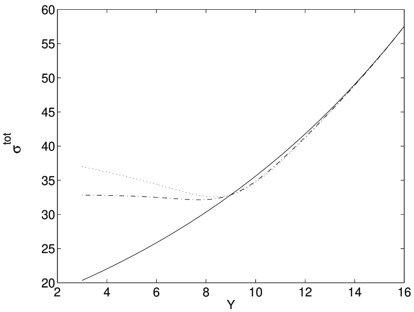
Figure 2: Effect of flavoring factor $R(s)$ when applied to a standard rising cross section: $\sigma^{cl}=\beta^{2}\>s^{\epsilon}$, $\epsilon=0.1$ and $\beta^{2}=16\>mb$, given by the solid curve. The dashed-dotted curve has $\epsilon_{o}=0$, $\lambda_{f}=1$, and flavoring scale $y_{f}=9$. The dotted curve corresponds to $\epsilon_{o}=-0.04$.

where $s_{f}\equiv e^{y_{f}}$. (See Figure 2.)

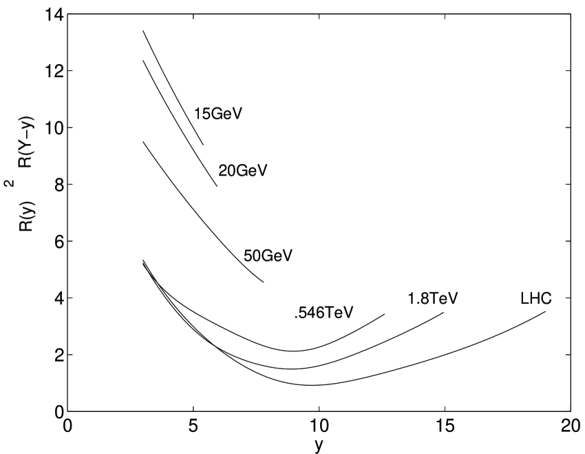
Figure 3: Renormalization factor due to flavoring alone, $Z_{f}(\xi;s)\equiv R^{2}(\xi^{-1})R(M^{2})$, as a function of rapidity $y=\log\xi^{-1}$ for various fixed center of mass energies.

This flavoring factor should be consistently applied as part of each “Pomeron propagator”. With the normalization $R(\infty)=1$, we can therefore leave the residues alone, once they have been determined by a “high energy” analysis. For instance, for the single-particle gap cross section before taking into account final-state screening, since there are three Pomeron propagators, one has for the renormalization factor $Z=R^{2}(y)R(y_{m})$. It is instructive to plot in Figure 3 this combination as a function of either $\xi$ or $M^{2}$ for various fixed values of $Y$.

5 Final Recipe

Having explained the notion of flavoring and its effects both on Pomeron intercept and on its residues, we need to go back to re-examine its effect for final-state screening. Since a Pomeron exchange enters as a Born term, i.e., the eikonal for either the elastic or the inelastic diffractive production, flavoring can easily be incorparated if we multiply both $\chi(y,b)$ and $\chi_{d}(y,b)$ by a flavoring factor $R(y)$. That is, if we adopt a generalized eikonal model for final-state screening, the desired screening factor becomes

$$S_{f}(\xi,t)=S_{f}^{(0)}(y,t;R(y)X(y),\mu_{d})$$ (32)

where $S_{f}^{(0)}$ is given by Eq. (16). Note that we have explicitly exhibited here the dependence on the maximal value of the flavored elastic eikonal, $RX$, and on the effectiveness parameter $\mu_{d}$.

Let’s now put all the necessary ingredients together and spell out the details for our proposed resolution to Dino’s paradox. Our final recipe for the Pomeron contribution to single diffraction dissociation cross section is

$${d\sigma\over dtd\xi}=D_{a,{\cal P}}(\xi,t)\Sigma_{{\cal P}b}(M^{2}),$$ (33)

where the unitarized flux, $D_{a,{\cal P}}$, and the Pomeron-particle cross section, $\Sigma_{{\cal P}b}$, are given in terms of their respective classical expressions by $D_{a,{\cal P}}(\xi,t)\equiv Z_{d}(\xi,t)F^{cl}_{a,\cal P}(\xi,t)$ and $\Sigma_{{\cal P}b}(M^{2})\equiv Z_{m}(M^{2})\Sigma^{cl}_{{\cal P}b}(M^{2}).$ It follow that the total suppression factor is

$$Z(\xi,t;M^{2})=Z_{d}(\xi,t)Z_{m}(M^{2})=[S_{f}(\xi,t)R^{2}(\xi^{-1})]R(M^{2}),$$ (34)

with the screening factor given by Eq. (32) and the flavoring factor given by Eq. (31). Finally, we point out that the integral constraint for the unitarized flux, Eq. (5), when written in terms of these suppression factors, becomes

$$\int_{-\infty}^{0}dt\int_{0}^{1}{d\xi}S_{f}(\xi,t)R^{2}(\xi^{-1})F_{a,{\cal P}}^{cl}(\xi,t)\xi^{\epsilon}=\beta_{a}^{diff}<\beta_{a}(0),$$ (35)

where $F_{a,{\cal P}}^{cl}(\xi,t)\equiv(1/16\pi)\beta_{a}(t)^{2}g(t)(\xi^{-1})^{2\alpha_{\cal P}(t)-1}$.

5.1 Phenomenological Parametrizations

Both the screening function and the flavoring function depend on the effective Pomeron intercept, and we shall adopt the following simple parametrization. The transition from $\alpha^{old}(0)=1+\epsilon_{o}$ to $\alpha^{new}(0)=1+\epsilon$ will occur over a rapidity range, $(y_{f}^{(1)},y_{f}^{(2)})$. Let $y_{f}\equiv{\textstyle{1\over 2}}(y_{f}^{(1)}+y_{f}^{(2)})$ and $\lambda_{f}^{-1}\equiv{\textstyle{1\over 2}}(y_{f}^{(2)}-y_{f}^{(1)})$. Similarly, we also define $\bar{\epsilon}\equiv{\textstyle{1\over 2}}(\epsilon+\epsilon_{o})$ and $\Delta\equiv{\textstyle{1\over 2}}(\epsilon-\epsilon_{o})$. A convenient parametrization for $\epsilon_{eff}$ we shall adopt is

$$\epsilon_{eff}(y)=[\bar{\epsilon}+{\Delta}\tanh{{\lambda_{f}}(y-\bar{y}_{f})}].$$ (36)

The combination $[{\epsilon-\epsilon_{eff}(y)}]$ can be written as $(2{\bar{\epsilon})\>[1+({s/s_{f}})^{2\lambda_{f}}]^{-1}}$ where $s_{f}=e^{y_{f}}$. Combining this with Eq. (31), we arrive at a simple parametrization for our flavoring function

$$R(s)\equiv\bigl{(}{s_{f}\over s}\bigr{)}^{(2\bar{\epsilon})\>[1+({s\over\bar{s}_{f}})^{2\lambda_{f}}]^{-1}}.$$ (37)

With $\alpha_{\cal P}^{old}\simeq 1$, we have $\epsilon_{o}\simeq 0$, $\bar{\epsilon}\simeq\Delta\simeq\epsilon/2$, and we expect that $\lambda_{f}\simeq 1\sim 2$ and $y_{f}\simeq 8\sim 10$ are reasonable range for these parameters. [27]

To complete the specification, we need to provide a more phenomenological description for the final-state screening factor. First, we shall approximate the screening factor by an exponential in $t$:

$$S_{f}(y,t)\simeq S_{f}(y,0)e^{\Delta B_{d}(y)t}.$$ (38)

where $S_{f}(y,0)=\{r\>x^{-r}\Gamma(x,r)\}^{2},$ with ${x=\mu_{d}R(y)X(y)}$ and $r=r(y)$. The width, $\Delta B_{d}(y)$, can be obtained by a corresponding substitution. Note that $S_{f}(y,0)$ depends on $B(y)$, $B_{d}(y)$, $X(y)$, and $\mu_{d}$. Phenomenological studies allow us to approximate $B(y)\simeq b_{0}+.25y$ and $B_{d}(y)\simeq b_{d}+.25y$, $b_{d}\simeq b_{0}/2\sim 2.3\>GeV^{-2}$.

The only quantity left to be specified is the effectiveness parameter $\mu_{d}$. Since the physics of final-state screening is that driven by a Pomeron with intercept greater than unity, the relevant rapidity scale is again $y_{f}$. Let us fix $\mu_{d}$ first by requiring that screening is small for $y<y_{f}$, i.e., $S_{f}(y,0)\sim 1$ as one moves down in rapidity from $y_{f}$ to $y_{r}$. Similarly, we expect screening to approach its full strength as one moves past the flavoring threshold $y_{f}$. We thus find it economical to parametrize

$$\mu_{d}(y)\simeq(\mu_{0}/2)\{1+\tanh[{\lambda_{d}(y-\bar{y}_{f})}]\},$$ (39)

and we expect $\lambda_{d}\sim\lambda_{f}$. This completes the specification of our unitarization procedure.

5.2 Qualitative Discussion

Before attempting to “use” our recipe, it is important to gain a qualitative understanding of what one can expect. Note that the sole effect of the flavoring factor $R$ is to “restore” a Pomeron contribution to that of a “bare Pomeron” with an intercept $\alpha^{old}_{\cal P}\simeq 1$. It follows that $R(y)\sim 1$ for $y>>y_{f}$ and $R(y)>1$ for $y<<y_{f}$. Similarly, since we expect final-state screening to increase as $\epsilon_{eff}(y)\sim\epsilon$, we therefore expect $S_{f}(y,t)<1$ for $y>>y_{f}$ and $S_{f}(y,t)\rightarrow 1$ for $y<<y_{f}$.

Let us examine the phase space region for a singly diffraction dissociation process from ISR to LHC. (See Figure 1.) It is customary to adopt $y\geq 3$ and ${y_{m}}\geq 0.4$ for a triple-Pmeron analysis, (corresponding to $\xi_{max}\sim 0.05$ and $\xi_{min}=1.5/s$.) However, a triple-Pomeron analysis cannot be reliably used for $0<y_{m}\leq y_{r}$. To be conservative, we adopt the same lower cutoff $y_{min}\simeq 3$ for both $y$ and $y_{m}$. With $y_{f}\simeq 8\sim 10$, the phase space is divided into the following four main regions of interest:

• (A) $y_{min}<y_{m}<y_{f}$, $y_{min}<y<y_{f}$:

  $\alpha_{eff}(y)\simeq 1$, $\alpha_{eff}(y_{m})\simeq 1$, and $d\sigma^{sd}/dy\sim constant$.

• (B) $y_{m}<y_{f}$, $y_{min}<y<y_{f}$:

  $\alpha_{eff}(y)\simeq 1$, $\alpha_{eff}(y_{m})\simeq 1+\epsilon$, and $d\sigma^{sd}/dy\sim e^{\epsilon y_{m}}=(M^{2})^{\epsilon}$.

• (C) $y_{min}<y_{m}<y_{f}$, $y>y_{f}$:

  $\alpha_{eff}(y)\simeq 1+\epsilon$, $\alpha_{eff}(y_{m})\simeq 1$, and $d\sigma^{sd}/dy\sim S_{f}(y,t)e^{2\epsilon y}=S_{f}(\xi,t)\xi^{-2\epsilon}$.

• (D) $y_{m}>y_{f}$, $y>y_{f}$:

  $\alpha_{eff}(y)\simeq 1+\epsilon$, $\alpha_{eff}(y_{m})\simeq 1+\epsilon$, and $d\sigma^{sd}/dy\sim S_{f}(y,t)e^{2\epsilon y}e^{\epsilon y_{m}}=S_{f}(\xi,t)\xi^{-\epsilon}s^{\epsilon}.$

In region-(A), diffractive cross sections behave according to the “old-fashion” Triple-Pomeron formula, with $\alpha_{\cal P}(0)=1$. Region-(B) is perhaps the best place where one has a clean chance of a direct detection of the $\epsilon>0$ effect coming from the $M^{2}$-dependence at fixed $y<y_{f}$. One would normally also expect to be able to detect the $\epsilon>0$ effect directly in Region-(C). However, in the large-$y$ limit where the strength of final-state screening becomes important,the suppression from $S_{f}(y,t)$ will overcome the $e^{2\epsilon y}$ behavior. Region-(D) exits only if $Y>2y_{f}$. With $y_{f}\simeq 8\sim 10$, this region becomes interesting only as one moves from Tevatron to LHC energies.

Consider the two available energies at Tevatron. Moving along a fixed $Y$ line, depending on the strength of screening, the cross section could be suppressed in the region-(C), and most of the contribution to $\sigma^{sd}$ will come from region-(A) and region-(B). As one moves from $\sqrt{s}=546\>GeV$ to $\sqrt{s}=1800\>GeV$, the rapidity span in region-B decreases. In contrast, below Tevatron energies, one is most likely to be in region-(A). Even more strikingly, at these “low energies”, a large portion of the kinematic region lies in regions where either $y$ or $y_{m}$ is near $y_{r}$ or below. As a consequence, we would not be surprised if our triple-Pomeron formula turns out to lead to a $\sigma^{sd}$ which is lower than what has been measured; other triple-Regge contributions should be included.

5.3 A Caricature of High Energy Diffractive Dissociation

The most important new parameter we have introduced for understanding high energy diffractive production is the flavoring scale, $s_{f}=e^{y_{f}}$. We have motivated by way of a simple model to show that a reasonable range for this scale is $y_{f}\simeq 8\sim 10$. Quite independent of our estimate, it is possible to treat our proposed resolution phenomenologically and determine this flavoring scale from experimental data.

It should be clear that one is not attempting to carry out a full-blown phenomenological analysis here. To do that, one must properly incorporate other triple-Regge contributions, e.g., the ${\cal PPR}$-term for the low-$y_{m}$ region, the $\pi\pi{\cal P}$-term and/or the ${\cal RRP}$-term for the low-$y$ region, etc., particularly for $\sqrt{s}\leq\sqrt{s_{f}}\sim 100\>GeV$. What we hope to achieve is to provide a “caricuture” of the interesting physics involved in diffractive production at collider energies through our introduction of the screening and the flavoring factors. [27]

Let us begin by first examining what we should expect. Concentrate on the triple-Pomeron vertex $g(0)$ measured at high energies. Let us for the moment assume that it has also been meassured reliably at low energies, and let us denote it as $g^{low}(0)$. Our flavoring analysis indicates that these two couplings are related by

$$g(0)\simeq e^{-({3\epsilon y_{f}\over 2})}g^{low}(0).$$ (40)

With $\epsilon\simeq 0.08\sim 0.1$ and $y_{f}\simeq 8\sim 10$, using the value $g^{low}(0)=0.364\pm 0.025\>\>mb^{{\textstyle{1\over 2}}}$, [14] we expect a value of $0.12\sim 0.18\>mb^{{\textstyle{1\over 2}}}$. Denoting the overall multiplicative constant for our renormalized triple-Pomeron formula by $K$,

$$K\equiv{\beta^{2}_{a}(0)g_{\cal PPP}(0)\beta_{b}(0)\over 16\pi}.$$ (41)

With $\beta^{2}_{p}\simeq 16\>mb$, we therefore expect $K$ to lie between the range $.15\sim.25\>\>mb^{2}$.

We begin testing our renormalized triple-Pomeron formula by first turning off the final-state screening, i.e., setting $S_{f}=1$. We determine the overall multiplicative constant $K$ by normalizing the integrated $\sigma^{sd}$ to the measured CDF $\sqrt{s}=1800\>GeV$ value.[28] With $\epsilon=0.1$, $\lambda_{f}=1$, this is done for a series of values for $y_{f}=7,\>8,\>9,\>10$. We obtain respective values for $K=.24,\>0.21,\>0.18,\>0.15,$ consistent with our flavoring expectation. As a further check on the sensibility of these values for the flavoring scales, we find for the ratio $\rho\equiv\sigma^{sd}(546)/\sigma^{sd}(1800)$ the values $0.63,\>0.65,\>0.68,\>0.72$ respectively. This should be compared with the CDF result of 0.834.

Next we consider screening. Note that screening would increase our values for $K$, which would lead to large values for $g$. Since we have already obtained values for triple-Pomeron coupling which are of the correct order of magnitude, the only conclusion we can draw is that, at Tevatron, screening cannot be too large. With our parametrization, we find that screening is rather small at Tevatron energies, with $\mu_{0}\simeq 0.0\sim 0.2$ This comes as somewhat a surprise! Clearly, screening will become important eventually at higher energies. After flavoring, the amount of screening required at Tevatron is apparently greatly reduced.

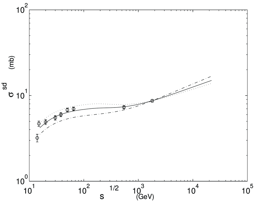
Figure 4: Various fits to representative single diffraction dissociation cross sections extracted from Ref. [5] from ISR to Tevatron. The solid line corresponds to $\epsilon=0.08$, $\epsilon_{o}=-0.07$, $\lambda_{f}=1$, $y_{f}=9$, with a small amount of final-state screening, $\mu_{0}=0.1$. The dotted curve corresponds to $\mu_{0}=0.2$, and the dashed-dotted curve corresponds to no screening, $\mu_{0}=0$.

Having shown that our renormalized triple-Pomeron formula does lead to sensible predictions for $\sigma^{sd}$ at Tevatron, we can improve the fit by enhancing the $PPR$-term as well as $RRP$-terms which can become important. Instead of introducing a more involved phenomenological analysis, we simulate the desired low energy effect by having $\epsilon_{o}\simeq-0.06\sim-0.08$. A remarkably good fit results with $\epsilon=0.08\sim 0.09$, $y_{f}=9$ and $\mu_{0}\simeq 0\sim 0.2$. [27] This is shown in Figure 4. The ratio $\rho$ ranges from $0.78\sim 0.90$, which is quite reasonable. The prediction for $\sigma^{sd}$ at LHC is $12.6\sim 14.8\>md$.

Our fit leads to a triple-Pomeron coupling in the range of

$$g_{\cal PPP}(0)\simeq.12\sim.18\>\>{mb}^{{\textstyle{1\over 2}}},$$ (42)

exactly as expected. Interestingly, the triple-Pomeron coupling quoted in Ref. [5] ($g(0)=0.69\>mb^{1\over 2}$) is actually a factor of 2 larger than the corresponding low energy value. [14] Note that this difference of a factor of 5 correlates almost precisely with the flux renormalization factor $N(s)\simeq 5$ at Tevatron energies.

We believe, with care, the physics of flavoring and final-state screening can be tested independent of the specific parametrizations we have proposed here. In particular, because our unitarized Pomeron flux approach retains factorization along the “missing mass” link, unambiguous predictions can be made for other processes involving rapidity gaps.

6 Predictions for Other Gap Cross Sections

For both double Pomeron exchange (DPE) and doubly diffractive (DD) processes, one is dealing with three rapidity variables which can become large. We will treat these two cases first before turning to more general situations.

Prediction for DPE Cross Sections:

For double Pomeron exchange (DPE), we are dealing with events with two large rapidity gaps. The final state configuration can be specified by five variables, $t_{1}$, $t_{2}$, $\xi_{1}$, $\xi_{2}$, and $M^{2}$. For $t_{1}$ and $t_{2}$ small, one again has a constraint, $\xi_{1}^{-1}M^{2}\xi_{2}^{-1}\simeq s$. Alternatively, we can work with rapidity variables, $y_{1}\equiv\log(\xi_{1}^{-1})$, $y_{2}\equiv\log(\xi_{2}^{-1})$, and $y_{m}\equiv\log M^{2}$, with $y_{1}+y_{m}+y_{2}\simeq Y=\log s$. The appropriate DPE differential cross section can be written down, with no new free parameter. Let us introduce a renormalization factor

$${d\sigma\over dy_{1}dt_{1}dy_{2}dt_{2}}=Z_{DPE}(y_{1},t_{1},y_{m},y_{2},t_{2}){d\sigma^{classical}\over dy_{1}dt_{1}dy_{2}dt_{2}}.$$ (43)

One immediately finds that, using Pomeron factorization for the missing mass variable,

$$Z_{DPE}=[S_{f}(y_{1},t_{1})R(y_{1})^{2}]R(y_{m})[S_{f}(y_{2},t_{2})R(y_{2})^{2}]=Z_{d}(\xi_{1},t_{1})Z_{m}(M^{2})Z_{d}(\xi_{2},t_{2}).$$ (44)

Alternatively, we can express this cross section in terms of singly diffractive dissociation cross sections as

$${d\sigma_{ab}\over dy_{1}dt_{1}dy_{2}dt_{2}}=\{{d\sigma_{ab}\over dy_{1}dt_{1}}\}\{R(y_{m})\sigma^{cl}_{{ba}}(y_{m})\}^{-1}\{{d\sigma_{ab}\over dy_{2}dt_{2}}\}$$ (45)

where $\sigma^{cl}_{{ba}}(y_{m})=\beta_{b}\beta_{a}e^{\epsilon\>y_{m}}$. This clean prediction involves no new parameter, with the understanding that, when $y_{m}$ is low, secondary terms must be added.

Prediction for DD Cross Sections:

For double diffraction dissociation (DD), there are two large missing mass variables, $M_{1}^{2}$, $M_{2}^{2}$, separated by one large rapidity gap, $y$, and its associate momentum transfer variable $t$. Again, for $t$ small, we have the constraint $y_{m_{1}}+y_{m_{2}}+y\simeq Y$.

The classical differential DD cross section is $\Sigma^{cl}_{a,{\cal P}}(y_{m_{1}}){\bar{F}}^{cl}_{{\cal P}}(y,t)\>\Sigma^{cl}_{b,{\cal P}}(y_{m_{2}}),$ where the classical “gap distribution” function is $\bar{F}^{cl}_{\cal P}(t,y)=(1/16\pi)e^{2(\epsilon+\alpha^{\prime}_{\cal P}t)y}g^{2}_{\cal PPP}(t).$ After taking care of both flavoring and final-state screening, on obtains for the renormalization factor

$$Z_{DD}(y_{m_{1}},y,t,y_{m_{2}})=R(M_{1}^{2})[\bar{S}_{f}(y,t)R(y)^{2}]R(M^{2})\equiv Z_{m}(M_{1}^{2})\bar{Z}_{d}(\xi,t)Z_{m}(M^{2}_{2}).$$ (46)

A new screening factor, $\bar{S}_{f}(y,t)$, has to be introduced because of the difference in the $t$-distribution associated with two factors of triple-Pomeron coupling. It can be obtained from $S_{f}(y,t)$ by replacing $B_{d}(y)$ by $\bar{B}(y)=\bar{b}+\alpha_{\cal P}^{\prime}t$, where, by factorization, $\bar{b}=2b_{d}-b_{0}$, ($\bar{b}$ is the t-slope associated with the triple-Pomeron coupling).

Alternatively, this cross section can again be expressed as a product of two single diffractive cross sections

$${d\sigma_{ab}\over dy_{m_{1}}dtdy_{m_{2}}}=\{{d\sigma_{ab}\over dy_{m_{1}}dt}\}\{\bar{Z}_{d}(y,t)\sigma^{el}_{ab}(y,t)\}^{-1}\{{d\sigma_{ab}\over dy_{m_{2}}dt}\},$$ (47)

where $\sigma^{el}_{ab}(y,t)\equiv(1/16\pi)|\beta_{a}(t)\beta_{b}(t)e^{(\epsilon+\alpha^{\prime}_{\cal P}t)y}|^{2}.$ Other than the modification from $S_{f}$ to $\bar{S}_{f}$, this prediction is again given uniquely in terms of the single diffraction dissociation cross sections.

Other Gap Cross Sections

We are now in the position to write down the general Pomeron contribution to the differential cross section with an arbitrary number of large rapidity gaps. For instance, generalizing the DPE process to an $n$-Pomeron exchange process, there will now be $n$ large rapidity gaps, with $n-1$ short-range ordered missing mass distributions alternating between two gaps. The corresponding renormalization factor is

$$Z^{(n)}_{PE}=Z_{d}(\xi_{1},t_{1})Z_{m}(M_{1}^{2})\bar{Z}_{d}(\xi_{2},t_{2})Z_{m}(M^{2}_{2})\cdots\cdots Z_{m}(M_{(n-1)}^{2})Z_{d}(\xi_{n},t_{n}).$$ (48)

Other generalizations are all straight forward. However, since these will unlikely be meanful phenomenologically in the near future, we shall not discuss them here. It is nevertheless interesting to point out that, if any cross section does become meaningful experimentally, flavoring would dictate that it is most likely the classical triple-Regge formulas with $\alpha_{\cal P}(0)\simeq 1$ that would be at work first.

7 Final Remarks:

Let us briefly recapitulate what we have accomplished. Given Pomeron as a pole, the total Pomeron contribution to a singly diffractive dissociation cross section can in principle be expressed as

$${d\sigma\over dtd\xi}=[S_{i}(s,t)][D_{a,{\cal P}}(\xi,t)][\Sigma_{{\cal P}b}(M^{2})],$$ (49)

$$D_{a,{\cal P}}(\xi,t)=S_{f}(\xi,t)F_{{\cal P}/a}(\xi,t)$$ (50)

• The first term, $S_{i}$, represents initial-state screening correction. We have demonstrated that, with a Pomeron intercept greater than unity and with a pole approximation for total and elastic cross sections remaining valid, initial-state absorption cannot be large. We therefore can justify setting $S_{i}\simeq 1$ at Tevatron energies.

• The first crucial step in our alternative resolution to the Dino’s paradox lies in properly treating the final-state screening, $S_{f}(\xi,t)$. We have explained in an expanding disk setting why a final-state screening can set in relatively early when compared with that for elastic and total cross sections.

• We have stressed that the dynamics of a soft Pomeron in a non-perturbative QCD scheme requires taking into account the effect of “flavoring”, the notion that the effective degrees of freedom for Pomeron is suppressed at low energies. As a consequence, we find that $F_{{\cal P}/a}(\xi,t)=R^{2}(\xi^{-1})F^{cl}_{{\cal P}/a}(\xi,t)$ and $\Sigma_{{\cal P}b}(M^{2})=R(M^{2})\Sigma_{{\cal P}b}^{cl}(M^{2})$ where $R$ is a “flavoring” factor.

It is perhaps worth contrasting what we have achieved with the flux renormalization scheme of Goulianos. [5] By construction, the normalization factor $N(s)$ is of the form which one would have obtained from an initial-state screening consideration. Although this breaks factorization, one might hope perhaps the scheme could be phenomenologically meaningful at Tevatron energies. Note that, for $\sqrt{s}>22$ $GeV$, the renormalization factor $N(s)$ has an approximately factorizable form: $N(s)\sim.25\>s^{2\epsilon}=.25\>(\xi^{-1})^{2\epsilon}(M^{2})^{2\epsilon}$. it follows that the diffractive differential cross section remains in a factorized form:

$$\xi{d\sigma^{sd}\over dtd\xi}\sim.25[\xi^{2\epsilon+1}F_{{\cal P}/p}^{(0)}(\xi,t)][(M^{2})^{-2\epsilon}\sigma_{{\cal P}p}^{(0)}(M^{2},t)].$$ (51)

It can be shown that Eq. (51) leads to a diffractive cross section $\sigma^{sd}$ which, up to $\log s$, is asymptotically constant. That is, the diffractive dissociation contribution no longer corresponds to the part of total cross sections represented by the Pomeron exchange. This is not in accord with the basic hypothesis of Pomeron dominance for total and elastic cross sections at Tevatron energies. [29]

Our final resolution shares certain common features with that proposed by Schlein. [8] At a fixed $\xi$, $Z_{m}(M^{2})\simeq 1$ as $s\rightarrow\infty$ so that it is possible to identify our renormalization factor $Z_{d}(\xi,t)=S_{f}(\xi,t)R^{2}(\xi^{-1})$ with the flux damping factor $Z_{S}(\xi)$ of Schlein. In Ref. [8], it was emphasized that the behavior of $Z_{S}(\xi)$ can be separated into three regions. (i) $(\xi_{1},\xi_{max})$ where $Z_{S}\simeq 1$, (ii) $(\xi_{2},\xi_{1})$ where $Z_{S}$ drops from 1 to 0.4 smoothly, and (iii) $(0,\xi_{2})$ where $Z_{S}(\xi)\rightarrow 0$ rapidly as $\xi\rightarrow 0$. The boundaries of these regions are $\xi_{1}\sim 0.015$ and $\xi_{2}\sim 10^{-4}$. The first bounday $\xi_{1}$ can be identified with our energy scale, $s_{r}$, $\xi_{1}^{-1}\sim y_{r}$. If we identify the boundary between region-(ii) and region-(iii) with our flavoring scale $y_{f}$ by $s_{f}^{-1}=e^{-y_{f}}=\xi_{2}$, one has $y_{f}\simeq 9$, which is consistent with our estimate. Since $S_{f}(\xi,t)\simeq 1$ for $\xi>s_{f}^{-1}$ and $R^{2}(\xi^{-1})$ drops from $R^{2}(1)\simeq s_{f}^{2\epsilon}$ to 1 at $s_{f}$, their $Z_{S}(\xi)$ behaves qualitatively like our renormalization factor. If one indeed makes this connection, what had originally been a mystery for the origin of the scale, $\xi_{2}$, can now be related to the non-perturbative dynamics of Pomeron flavoring. [30]

It should be stressed that our discussion depends crucially on the notion of soft Pomeron being a factorizable Regge pole. This notion has always been controversial. Introduced more than thirty years ago, Pomeron was identified as the leading Regge trajectory with quantum numbers of the vacuum with $\alpha(0)\simeq 1$ in order to account for the near constancy of the low energy hadronic total cross sections. However, as a Regge trajectory, it was unlike others which can be identified by the particles they interpolate. With the advent of QCD, the situation has improved, at least conceptually. Through large-$N_{c}$ analyses and through other non-perturbative studies, it is natural to expect Regge trajectories in QCD as manifestations of “string-like” excitations for bound states and resonances of quarks and gluons due to their long-range confining forces. Whereas ordinary meson trajectories can be thought of as “open strings” interpolating $q\bar{q}$ bound states, Pomeron corresponds to a “closed string” configuration associated with glueballs. However, the difficulty of identification, presummably due to strong mixing with multi-quark states, has not helped the situation in practice. In a simplified one-dimensional multiperipheral realization of large-N QCD, the non-Abelian gauge nature nevertheless managed to re-emerge through its topological structure. [24][25]

The observation of “pole dominance” at collider energies has hastened the need to examine more closely various assumptions made for Regge hypothesis from a more fundamental viewpoint. It is our hope that by examining Dino’s paradox carefully and by finding an alternative resolution to the problem without deviating drastically from accepted guiding principles for hadron dynamics, Pomeron can continued to be understood as a Regge pole in a non-perturbative QCD setting. The resolution for this paradox could therefore lead to a re-examination of other interesting questions from a firmer theoretical basis. For instance, to be able to relate quantities such as the Pomeron intercept to non-perturbative physics of color confinement represents a theoretical challenge of great importance.

Acknowledgments: I would like to thank K. Goulianos for first getting me interested in this problem during the Aspen Workshop on Non-perturbative QCD, June 1996. Intensive discussions with K. Goulianos, A. Capella, and A. Kaidalov at Rencontres de Moriond, March, 1997, have been extremely helpful. I am also grateful to P. Schlein for explaining to me details of their work and for his advice. I want to thank both K. Goulianos and P. Schlein for helping me to understand what I should or should not believe in various facets of diffractive data! Lastly, I really appreciate the help from K. Orginos for both numerical analysis and the preparation for the figures. This work is supported in part by the D.O.E. Grant #DE-FG02-91ER400688, Task A.

References

- [1] This is the first of a series of papers where we discuss the general subject of diffraction scattering at Tevatron energies. In this first article, we concentrate on soft diffractive production. In a subsequent article, we shall discuss the relation between soft and hard Pomeron, [3] with particular emphasis on the “flavoring” mechanism leading to the picture of a “Heterotic Pomeron”, (hep-ph/9302308).
- [2] For fits for soft Pomeron parameters, see: A. Donnachie and P. V. Landshoff, Phys. Lett. B 296 (1992) 227; J. R. Cuddel, K. Kang, and S. K. Kim, Phys. Lett., B 395 (1997) 311; R. J. M. Covolan, J. Montanha, and K. Goulianos, Phys. Lett., B 389 (1996) 176; M. Block, to be presented at VIIth Blois Workshop on Elastic and Diffractive Scattering, Seoul, June 10-14, 1997.
- [3] G. Ingelman and P. Schlein, Phys. Lett. B 296 (1992) 227.
- [4] We use as the basic energy scale through out this paper. These “classical” expressions are: and The triple-Pomeron coupling can be in principle determined by data below where cross sections are relatively insensitive to the choice of the Pomeron intercept value used. As far as I am aware of, the first attempt in using a “triple-Regge” analysis to interpret real experimental data was made by: D. Silverman and C-I Tan, “Relation Between the Multi-Regge Model and the Missing-Mass Sepctrum”, Phys. Rev., D2 (1970) 233. A formal postulation was first made by DeTar, Jones, Low, Tan, Weis, and Young, Phys. Rev. Letters, 26 (1971) 675. For other contemporaneous works, see: D. Horn and F. Zachariasen, “Hadron Physics at Very High Energies”, (Benjamin, 1973).
- [5] K.Goulianos, Phys. Lett., B 358 (1995) 379.
- [6] With , , , , for , and for where .
- [7] K. Goulianos, Proceedings of the 3rd Workshop on Small-x and Diffractive Physics, Argonne National Laboratory, USA, September 1996; K. Goulianos, Proceedings of the 5th International Workshop on Deep Inelastic Scattering and QCD (DIS-97), Chicago, USA, April 1997.
- [8] P. Schlein, Proceedings of the 3rd Workshop on Small-x and Diffractive Physics, Argonne National Laboratory, USA, September 1996; P. Schlein, Proceedings of the 5th International Workshop on Deep Inelastic Scattering and QCD (DIS-97), Chicago, USA, April 1997.
- [9] S. Erhan and P. Schlein, “Saturation of the Pomeron Flux Factor in the Proton by Damping Small Pomeron Momenta”, to be submitted to Phys. Lett. For a difference in opinion, see Ref. [10]. See also: A. Brandt, et al., “Measurements of Single Diffraction at GeV; Implication for the Pomeron Flux Factor”, to be submitted to Nucl. Phys.
- [10] K. Goulianos, “Comments on the Erhan-Schlein Model of Damping the Pomeron Flux at Small-x”, hep-ph/9704454.
- [11] When compared with the classical formula, our decomposition corresponds to having the triple-Regge coupling absorbed into the flux factor, . For our subsequent discussion, the triple-Pomeron coulping will be absorbed into the classical flux factor and the Pomeron-particle cross section without will be denoted by .
- [12] C-I Tan, Proc. of 2nd International Conference on Elastic and Diffractive Scattering, ed. K. Goulianos, (Editions Frantieres, 1987) p347.
- [13] C-I Tan, Proc. of XIXth International Symposium on Multiparticle Dynamics, Arles, ed. D Schiff and J. Tran T. V. (Editions Frontieres, 1988) p361.
- [14] R. L. Cool, K. Goulianos, S. L. Segler, H. Sticker and S. N. White, Phys. Rev. Lett. 47 (1981) 701.
- [15] For diffraction dissociation, must have same quantum numbers as the incident particle . For definiteness, we discuss leading particle gap distribution relative to the incoming particle with a positive, large rapidity, and assume . For collision, actual diffractive cross section, , is arrived at by taking into account contributions involving diffraction at both and vertices.
- [16] This mechanism has been recognized before. It was used in Refs. [13] and [17] to explain why a “maximal odderon” cannot be allowed in any hadronic scheme which admits an expanding-disk interpretation at high energies.
- [17] G. Finkelstein, H. M. Fried, K. Kang, and C-I Tan, Phys. Lett., B 232 (1989) 257.
- [18] W. Frazer, D. R. Snider and C-I Tan, Phys. Rev., D8 (1973) 3180.
- [19] It is possible also to apply an eikonal model to study initial state screen for singly diffractive dissociation cross section. This indeed has been performed before, however, without taking final-state screening into account. [20] The fact that inelastic absorption takes place at small impact parameter, with surviving scattering allowed only at the edge of the expanding disk has also been noted there. Since our final-state absorption would remove all scattering within the disk, applying an eikonal initial-state absorption procedure becomes unnecessary.
- [20] E. Gotsman, E. M. Levin, and U. Maor, Phys. Rev., D49 (1994) 4321.
- [21] T. K. Gaisser and C-I Tan, Phys. Rev., D8 (1973) 3881.
- [22] C-I Tan, Proc. IX Rencontres de Moriond, Meribel, France (1974).
- [23] We include both and production as well as other effects. The effective degrees of freedom involved are “diquarks” and charm quarks respectively. For color counting, a baryon is considered as a bound state of a quark and diquark. See also: J. W. Dash and S. T. Jones, Phys. Lett., B 157 (1985) 229.
- [24] H. Lee, Phys. Rev. Lett., 30 (1973) 719; G. Veneziano, Phys. Lett., B 43 (1973) 314. See also, F. Low, Phys. Rev. D 12 (1975) 163.
- [25] A phenomnenological realization of QCD emphasizing the topological structure of large-N gauge theories is Dual Parton Model, (DPM). For a recent review, see: A. Capella, U. Sukhatme, C-I Tan, and J. Tran T. V., Physics Reports, 236 (1994) 225.
- [26] We do not include “semi-hard” production in the current treatment for soft Pomeron. Flavoring will indeed be the primary mechanism in our construction of a “Heterotic Pomeron”. As mentioned in Ref. [1], this will be treated in a separate publication.
- [27] By choosing , it is possible to provide a global “average” description mimicking “secondary trajectory” contributions for various low energy regions. In Ref. [21], acceptable estimates are .
- [28] The published CDF values at and are and respectively. These values correspond to . We shall restrict and to be inside the extreme forwrad peak. For , we reduce these values by while maintaining their relative ratio of . For to be within the extreme forward diffraction peak we scale down the ISR diffractive cross sections also by approximately . This is appropriate for our determination of the triple-Pomeron coupling.
- [29] Ultimately, these two schemes can be differentiated by confronting experimental data. For our scheme, because of Pomeron pole dominance, it leads to a normalizable limiting gap distribution, , i.e., For , it is cut-off in at least as fast as In contrast, the flux renormalization scheme, Eq. (51), leads to a gap distribution of the form for . Test of these two alternatives for either the normalization and the -distribution can in principle be carried out by comparing data at two Tevatron energies by focusing on the region of fixed small and , (). Unfortunately, both behaviors seem to provide acceptable fits based on data presented in Ref. [10].
- [30] There are also several differences between our result and that of Schlein. First, our renormalization factor is t-dependent whereas Schlein’s is not. At very small , our suppression factor does not vanish as fast as that of Schlein: , whereas ours behaves as . Furthermore, since we have found that there is very little screening needed at Tevatron energies, our slow cutoff might not set in until much higher energies so that it could indeed be possible to observe the behavior for in Region-(C) at Tevatron energies.