Phenomenology of Deep Inelastic Scattering Structure Functions

Abstract

I review recent progress in analysing deep inelastic scattering structure functions in global analyses. The new ingredients are new data and attempts to incorporate heavy quarks consistently. A new way of including the resummation of large $\log 1/x$ terms is discussed.

Introduction

Since we last met in Rome last year there has been progress in our understanding of deep inelastic scattering (DIS) structure functions and the implications of new measurements in the context of global analyses and extraction of parton distribution functions (pdf’s). Firstly there have been updates to two major experiments $-$ the muon-nucleon NMC collaboration at CERN and the neutrino-iron CCFR collaboration at Fermilab. The NMC nmc has produced their final numbers for $F_{2}$ for proton and deuterium targets at 90, 120, 200 and 280 GeV while the CCFR ccfr collaboration has implemented new energy calibrations to its analysis. The latter data are consistent with a greater value of $\alpha_{s}(M_{Z})$ than the previously reported value. Finally there have been the first reported measurements from HERA on the charm structure function $F_{2}^{c}$ charmh1 ; charmzeus which indicate that a substantial fraction of the total $F_{2}$ at HERA comes from charm production.

On the theoretical side, progress has been made following improved treatments of heavy quark production in DIS. Why is this important? From above we see that the component of $F_{2}$ is relatively large and so it is obviously important to have a consistent description of this component and to check this with boson-gluon fusion mechanisms. Also if we are trying to understand the small $x$ behaviour of $F_{2}$ (i.e. BFKL versus GLAP) then the data force us to study small $Q^{2}$ i.e. the region where we move through the charm threshold; so this should be understood. Finally it is necessary to produce pdf’s for charm and bottom flavours to insert into other processes such as jet production.

Large $x$, high $Q^{2}$ is where the excitement resides just now. Can we be precise about the conventional background and estimate the uncertainty in the cross section around $Q^{2}\sim 10^{5}GeV^{2}$, $x\sim 0.45$? I shall discuss this briefly.

For some time it has been realised that in addition to resumming large logs in $Q^{2}$ (GLAP), there may be significant contributions arising from resumming potentially large logs in $1/x$ (BFKL). The difficulty is to devise a theoretically consistent procedure of ‘ marrying’ the two in a practical way that confronts the data and tries to answer the question whether these data favour or disfavour the inclusion of the $\log 1/x$ resummed terms. Here there has been definite progress and I shall highlight a recent analysis by Thorne thorne .

Recent global analyses

The two major providers of pdf’s, CTEQ and MRS, continue to update their global analyses of DIS and other processes. Both are now attempting to include a theoretically improved treatment of charm and bottom and these treatments are discussed in the following section. In this section I will highlight some results emerging from these on-going analyses.

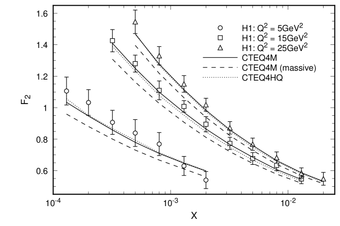
Figure 1: Comparison of H1 datah1f2 with calculations using CTEQ4M pdf’s in the original massless scheme (solid line) with the new fit CTEQ4HQ using the ACOT procedure (dotted line).

Lai and Tunglai demonstrate the effect of including the variable flavour scheme (VFNS) developed by Aivazis et al.acot (ACOT) based on their ealier workwkt into the CTEQ analysis. This is to be contrasted with the previous treatment in CTEQ where charm evolved as a massless quark. The effect is illustrated in fig. 1.

Only a small change is observed as one changes from CTEQ4M (the massless evolution) to the improved VFNS procedure which is more noticeable at small $x$. A comparison of the resulting pdf’s at $Q^{2}=25$ GeV² is shown in fig. 2

Figure 2: Comparison of CTEQ4M and CTEQ4HQ pdf’s

Moreover, the quality of the resulting fit to the full $F_{2}$ is improved at low $x$.

The series of global analyses carried out by MRS has been updated. The new data from NMCnmc and CCFRccfr are included and the improved treatment of the heavy quark developed by Martin et al.mrrs is used (see next section). As with the previous MRS analysismrsr a low value of the starting scale $Q_{0}^{2}$ of 1 GeV² is taken. This is mainly to reach as small $x$ as possible for the HERA datah1f2 ; zeusf2 for which a cut at $Q^{2}=1.5$ GeV² is taken while the cut is at 2 GeV² for other DIS data. In order to study the sensitivity to the value of $\alpha_{s}(M_{Z})$, the analysis is repeated at fixed values of $\alpha_{s}(M_{Z})$ over a wide range. The resulting values of the individual $\chi^{2}$ values for the DIS data sets are shown in fig. 3.

Figure 3: Values of $\chi^{2}$ for various DIS datasetsh1f2 ; zeusf2 ; bcdms ; nmc ; slac ; e665 as $\alpha_{s}(M_{Z})$ is varied

From the figure we see (i) that the HERAh1f2 ; zeusf2 data prefer a value of $\alpha_{s}(M_{Z})$ around 0.12 or sobf1 , (ii) that the updated NMCnmc data also prefer this somewhat larger value and (iii) the re-analysed CCFRccfr $F_{2}$ data strongly favour a value at the upper end. This leaves BCDMSbcdms data as the one set which still favours a relatively low value of $\alpha_{s}(M_{Z})$. But we should recall that these data are very precise and measure scaling violations in the large $x$ region where the determination of $\alpha_{s}(M_{Z})$ is insensitive to possible uncertainty of the gluon distribution.

The resulting best value of $\alpha_{s}(M_{Z})$ which emerges from this overall global analysis is 0.118 and we show comparisons of the fit using this value with a selection of data. The small $x$ data comparison is shown in fig. 4.

Figure 4: Comparison of the new fit using $\alpha_{s}(M_{Z})=0.118$ with the small $x$ data from refsh1f2 ; zeusf2 ; e665 .

The comparsion with the new NMC data is shown in fig. 5.

Figure 5: Comparison of the new fit using $\alpha_{s}(M_{Z})=0.118$ with the NMC datanmc .

Notice that points below $Q^{2}=2$ GeV², while shown in the figure, were not included in the fit. Finally we show the comparison with the new data from CCFRccfr on $F_{2}$ extracted from $\nu$ and $\bar{\nu}$ interactions off an iron target in Fig. 6.

Figure 6: Comparison of the new fit using $\alpha_{s}(M_{Z})=0.118$ with the new CCFRccfr data on $F_{2}$. Here the theory curves have been multiplied by a heavy target $x$ dependent correction factor and only the statistical errors are shown on the data.

The failure to agree below $x$ of around 0.1 is well known. Basically these low $x$ data prefer not to have the shadowing corrections, observed in muon DIS, applied. Because of this conflict (with the NMC data for example) CCFR $F_{2}$ below $x=0.1$ is dropped in the fit. Comparing the curves and large $x$ data in fig. 6 one can see that the data prefer slightly stronger $Q^{2}$ variation than that from using $\alpha_{s}(M_{Z})=0.118$. Much better consistency is found for $xF_{3}$ across the entire $Q^{2}$, $x$ range.

In this analysis, the pdf’s at $Q_{0}^{2}$ are parametrised in the usual MRSmrsr way with $xg(x,Q_{0}^{2})\sim x^{-\lambda_{g}}$ and $xS(x,Q_{0}^{2})\sim x^{-\lambda_{s}}$ for the glue and sea as $x\rightarrow 0$. The exponents $\lambda_{g}$ and $\lambda_{s}$ are not constrained and as in the previous analysis one finds that at such a low choice of $Q_{0}^{2}=1$ GeV² $\lambda_{s}$ is positive (singular) while $\lambda_{g}$ comes out negative $-$ i.e ‘valence-like’ gluon. The actual value of the exponent varies for different values of $\alpha_{s}(M_{Z})$ ($-0.15$ to $-0.21$) but when $Q^{2}$ reaches just 2 GeV² all the gluon pdf’s are approximately ‘flat’, see fig. 7.

Figure 7: Gluon distribution functions at $Q^{2}=2$ GeV² as $\alpha_{s}(M_{Z})$ is varied from 0.105 (upper dashed) through 0.110 (dot-dashed), 0.115 (upper dotted), 0.1175 (upper solid), 0.120 (lower dashed), 0.125 (lower solid) and 0.1275 (lower dotted).

Taking the fit with $\alpha_{s}=0.118$ and evolving to $Q^{2}=25$ GeV² yields pdf’s which are extremely close to those shown in fig. 2 so the different treatments of charm partons in the latest analyses of CTEQ and MRS actually lead to little numerical difference in the resulting pdf’s.

Theoretical discussion of heavy quark production in DIS

Let us consider possible approaches to treating the charm production contribution to the structure function $F_{2}$.

Massless parton evolution

The most simplistic approach is to assume that a probe of virtuality $Q^{2}$ can resolve a charm quark pair in the proton sea when $Q^{2}\lower 3.01385pt\hbox{$\;\stackrel{{\scriptstyle\textstyle>}}{{\sim}}\;$}m_{c}^{2}$. Since such pairs originate from fluctuations of the gluon field, $g\to c\overline{c}$, a perturbative treatment should be valid as long as $m_{c}^{2}\gg\Lambda_{QCD}^{2}$. As $Q^{2}$ increases, ${\cal O}(m_{c}^{2}/Q^{2})$ corrections to the standard GLAP evolution become less important, and the charm quark can be treated as a (fourth) massless quark. These ideas are embodied in the ‘massless parton evolution’ (MPE) approach

$$c(x,Q^{2}) = 0\quad\mbox{for}\quad Q^{2}\leq\mu_{c}^{2}\;,$$

$$n_{f} = 3+\theta(Q^{2}-\mu_{c}^{2})\quad\mbox{in}\quad P_{qg},\;P_{gg},\;\beta_{0},\ldots\;,$$ (1)

where $\mu_{c}={\cal O}(m_{c})$. The charm contribution to the structure function is then

$$F_{2}^{c}(x,Q^{2})=\textstyle{\frac{8}{9}}xc(x,Q^{2})$$ (2)

in lowest order. This is the approach adopted at NLO in the MRS and CTEQ global parton analyses, with $\mu_{c}$ chosen in the MRS analysis to achieve a satisfactory description of the EMC $F_{2}^{c}$ data emccharm , while in the CTEQ analysis $\mu_{c}$ is set equal to $m_{c}$. For example, in the MRS(A) analysis mrsa it was found that $\mu_{c}^{2}=2.7$ GeV² and that this was to a good approximation equivalent to taking

$$2c(x,Q_{0}^{2})\;=\;\delta{\cal S}(x,Q_{0}^{2})$$ (3)

with $\delta\approx 0.02$ at the input scale $Q_{0}^{2}=4$ GeV². That is at the input scale, charm $(c+\overline{c})$ was found to have approximately the same shape as the total quark sea distribution ${\cal S}$, and moreover to form about 2% of its magnitude.

In NLO the charm structure function is given by

$$F_{2}^{c}(x,Q^{2})\;=\;\frac{8}{9}\>\int_{x}^{1}\>dz\>\frac{x}{z}\>\left[C_{q=c}(z,Q^{2},\mu^{2})\>c\left(\frac{x}{z},\mu^{2}\right)\>+\>C_{g}(z,Q^{2},\mu^{2})\>g\left(\frac{x}{z},\mu^{2}\right)\right]$$ (4)

The charm quark coefficient function in (4) has the form

$$C_{c}\;=\;C_{c}^{(0)}\>+\>\frac{\alpha_{S}}{4\pi}\>C_{c}^{(1)}\>+\>\ldots,$$ (5)

while for the gluon we have

$$C_{g}\;=\;\frac{\alpha_{S}}{4\pi}\>C_{g}^{(1)}\>+\>\ldots\>$$ (6)

and this expression with the standard massless $\overline{\rm MS}$ coefficient functions was used to calculate $F_{2}^{c}$ in the MPE approach.

Boson-gluon fusion

A procedure which takes a very different approach is to generate $F_{2}^{c}$ from photon-gluon fusion (PGF) ghr ; grs alone. In this case, the charm pdf appearing in eq.(4) is identically zero everywhere but the gluon coefficient function involves the non-zero charm mass $m_{c}$ and is the well-known PGF cross section, i.e. $C_{g}^{1}(z)\rightarrow C_{g}^{\rm PGF}(z,Q^{2})$ with

$$C_{g}^{\rm PGF}(z,Q^{2})=\left\{\left[z^{2}\>+\>(1-z)^{2}\>+\>\frac{4m_{c}^{2}}{Q^{2}}\>z(1-3z)\>-\>\frac{8m_{c}^{4}}{Q^{4}}\>z^{2}\right]\right.\>\ln\>\frac{1+\beta}{1-\beta}$$

$$+\;\left.\left[8z(1-z)\>-\>1\>-\>\frac{4m_{c}^{2}}{Q^{2}}\>z(1-z)\right]\>\beta\right\}\;\Theta\left(Q^{2}\>\left(\frac{1}{z}-1\right)\>-\>4m_{c}^{2}\right).$$ (7)

where $\beta$ is the velocity of one of the charm quarks in the photon-gluon centre-of-mass frame

$$\beta^{2}\;=\;1\>-\>\frac{4m_{c}^{2}\>z}{Q^{2}(1-z)}.$$ (8)

The $\Theta$ function in eq.(7), $\Theta(W^{2}-4m_{c}^{2})$, represents the $c\overline{c}$ production threshold, where $W$ is the c.m. energy. Its presence guarantees $\beta^{2}\geq 0$. The exact next-to-leading order corrections to the PGF structure function are known lvn and recently bmsvn1 an analysis has been used to perform $(\alpha_{S}\ln(Q^{2}/m_{c}^{2}))^{n}$ resummation up to ${\cal O}(\frac{m_{c}^{2}}{Q^{2}})$ for $Q^{2}\gg m_{c}^{2}$. Such an approach is of course not applicable in the threshold region $Q^{2}\lower 3.01385pt\hbox{$\;\stackrel{{\scriptstyle\textstyle>}}{{\sim}}\;$}m_{c}^{2}$. However for many purposes the PGF procedure is insufficient. If we consider the high $Q^{2}$ limit of $C_{g}^{PGF}$ we get

$$C_{g}^{\rm PGF}\;\rightarrow\;\left\{z^{2}\>+\>(1-z)^{2}\right\}\;\ln\left(\frac{1-z}{z}\;\frac{Q^{2}}{m_{c}^{2}}\right)\>+\>8z(1-z)-1$$ (9)

as $m_{c}\rightarrow 0$, which differs from the exact $m_{c}=0$ coefficient $C_{g}^{(1)}$ by the presence of $Q^{2}/m_{c}^{2}$ in the argument of the logarithm. This is a signal of potentially large logs which should be resummed by GLAP evolution. Thus at large $Q^{2}$ we should include the charm quark as a parton in GLAP evolution. In fact we should be able to provide a charm pdf all the way down to the charm threshold in order to insert all relevant pdf’s into calculations of other perturbative QCD processes. The goal therefore is to do this in a consistent way

Variable flavour number scheme procedure

Here the procedure is to have no charm pdf below $Q^{2}=m_{c}^{2}$ but for $Q^{2}\geq m_{c}^{2}$ to have $c+\bar{c}\sim\alpha_{s}P_{qg}\ln Q^{2}/m_{c}^{2}$, where $P_{qg}$ is the splitting function $g\rightarrow c\bar{c}$ evaluated with $m=0$. Below $Q^{2}=m_{c}^{2}$ charm is produced solely by boson-gluon fusion as above and this is labelled the ‘fixed flavour number’ scheme (FFNS). Thus for $n_{f}=3$ we have an OPE for the structure functions

$$F=C_{FFNS}\left(\frac{Q^{2}}{\mu^{2}},\frac{m_{c}^{2}}{\mu^{2}},\alpha_{s}(\mu^{2})\right)\;\hat{O}_{FFNS}(\alpha_{s}(\mu^{2}))\;+\;{\cal O}(\frac{\Lambda^{2}}{Q^{2}})$$ (10)

Above $Q^{2}=m_{c}^{2}$ we work in the ‘variable flavour number’ scheme (VFNS) with $n_{f}=4$ and write the OPE

$$F=C_{VFNS}\left(\frac{Q^{2}}{\mu^{2}},\alpha_{s}(\mu^{2})\right)\;\hat{O}_{VFNS}(\frac{Q^{2}}{\mu^{2}},\frac{m_{c}^{2}}{\mu^{2}},\alpha_{s}(\mu^{2}))\;+\;{\cal O}(\frac{m_{c}^{2}}{Q^{2}})$$ (11)

While the operators $\hat{O}_{VFNS}$ nominally depend on $m_{c}^{2}$ they can be chosen so that they evolve according to $m=0$ RGE’s. Thus in the VFNS the $m_{c}^{2}$ dependence appears only in the corrections. The coefficients $C_{VFNS}$ are simply the usual massless $\overline{\rm MS}$ coefficients $C_{\overline{\rm MS}}$. The two schemes must be mutually consistent at all $Q^{2}>m_{c}^{2}$ which implies (from eqns.(10,11)) that the ${\cal O}(\frac{m_{c}^{2}}{Q^{2}})$ contribution in eq.(11) can be written in the form

$$C^{\prime}(\frac{m_{c}^{2}}{\mu^{2}})\;\hat{O}_{FFNS}(\alpha_{s}(\mu^{2}))\;\;+\;\;{\cal O}(\frac{\Lambda^{2}}{\mu^{2}})$$ (12)

where $C^{\prime}$ is a coefficient which $\sim$ powers of $\frac{m_{c}^{2}}{\mu^{2}}$. If we express the relation between the operators of the two schemes through a matrix $A$,

$$\hat{O}_{VFNS}=A\left(\frac{m_{c}^{2}}{\mu^{2}},\alpha_{s}(\mu^{2})\right)\;\hat{O}_{FFNS}(\alpha_{s})$$ (13)

then, in particular, the charm pdf is determined purely in terms of the light parton pdf’s $-$ principally the gluon distribution of course. The structure functions above $Q^{2}=m_{c}^{2}$ can again be expressed in terms of the VFNS operators but now up to ${\cal O}(\frac{\Lambda^{2}}{Q^{2}})$ corrections,

$$F = \left[C_{VFNS}\left(\frac{Q^{2}}{\mu^{2}},\alpha_{s}\right)+C^{\prime}(\frac{m_{c}^{2}}{\mu^{2}})A^{-1}\right]\;\hat{O}_{VFNS}\;+\;{\cal O}(\frac{\Lambda^{2}}{Q^{2}})$$ (14)

$$= C_{ACOT}\left(\frac{Q^{2}}{\mu^{2}},\frac{m_{c}^{2}}{\mu^{2}},\alpha_{s}\right)\hat{O}_{VFNS}\;+\;{\cal O}(\frac{\Lambda^{2}}{Q^{2}})$$

where $C_{ACOT}$ is the coefficient in the ACOTacot ; wkt formalism which then depends on $m_{c}^{2}$. Thus in the ACOT formalism, while the partons obey a simple evolution (independent of $m_{c}^{2}$), the coefficients would have a complicated dependence on $m_{c}^{2}$. From eqns (10,14) we obtain the relation between the coefficient functions

$$C_{ACOT}\left(\frac{Q^{2}}{\mu^{2}},\frac{m_{c}^{2}}{\mu^{2}},\alpha_{s}\right)=C_{VFNS}\left(\frac{Q^{2}}{\mu^{2}},\alpha_{s}\right)+C^{\prime}(\frac{m_{c}^{2}}{\mu^{2}})A^{-1}\;=C_{FFNS}\left(\frac{Q^{2}}{\mu^{2}},\frac{m_{c}^{2}}{\mu^{2}},\alpha_{s}\right)A^{-1}$$ (15)

where the term $C^{\prime}A^{-1}$ on the rhs $\rightarrow 0$ as $Q^{2}\rightarrow\infty$.

Buza et al.bmsvn1 have evaluated the coefficient functions for $Q^{2}\gg m_{c}^{2}$ in the VFNS and the FFNS to NLO. They find that for $Q^{2}\lower 3.01385pt\hbox{$\;\stackrel{{\scriptstyle\textstyle>}}{{\sim}}\;$}20{\rm GeV}^{2}$ the two schemes agree very closely. The same authors have worked out the relation (13) in the limit $Q^{2}\gg m_{c}^{2}$ exactly through terms $\ln^{2}(m_{c}^{2}/\mu^{2})$, $\ln(m_{c}^{2}/\mu^{2})$ and constants. This infers a matching of all the four flavour pdf’s above the scale $\mu^{2}=m_{c}^{2}$, to the three flavour pdf’s below. Again this is only for $Q^{2}\gg m_{c}^{2}$, which does not solve the problem of what to do at $Q^{2}\sim m_{c}^{2}$. So there has to be another matching between the calculated $c\overline{c}$ production cross section in the threshold region to the charm pdf prescription at $Q^{2}\gg m_{c}^{2}$. In leading order this is exactly the ACOT procedure. It remains to be investigated how to do this retaining terms ${\cal O}(m_{c}^{2}/Q^{2})$ at NLO.

Thus although the ${\rm FFNS}\rightarrow{\rm VFNS}$ change of factorization scheme is very attractive in principle, a major problem arises when one tries to go down in $Q^{2}$ (still at NLO) all the way to the charm threshold - retaining the $C^{\prime}A^{-1}$ term $-$ which is the eventual aim of ACOT. The $A^{-1}$ term is the one which contains the subtraction in the gluon coefficient functions for $F^{C}_{2}$ in eq.(2) to avoid double counting which at LO is quite straightforward and takes the form

$$C_{g}^{(1)}(z)=C^{PGF}_{g}(z)-\alpha_{s}C_{c}^{(0)}\times P_{qg}^{(0)}\ln Q^{2}/m_{c}^{2}$$

The effect of this is that $F^{c}_{2}$ is described at low $Q^{2}$ by PGF but as $Q^{2}\rightarrow\infty$ by the evolved charm pdf.

Since the way it has been formulated is only at leading order (the charm pdf evolves only via $P^{(0)}_{qg}(z)$) this allows the standard expression to be used for the gluon coefficient function. We are still left with the problem of how to evolve all the pdf’s beyond L.O. - in the $\overline{\rm MS}$ scheme say. While the splitting functions will continue to have the $m=0$ forms, the entire $m^{2}$ dependence is put into the coefficient functions which will make them (the light parton coefficient functions as well as the charm coefficient functions) extremely complicated when they are eventually computed.

MRRS procedure

In view of the practical difficulties of implementing the ACOT procedure at NLO, Ryskin and MRSmrrs introduce an alternative prescription which is consistent at all orders but which generates partons which may be used with the conventional $\overline{\rm MS}$ coefficient functions. The charm quark evolution is modified however $-$ of course only for $Q^{2}\gg m_{c}^{2}$ does it evolve according to the massless $\overline{\rm MS}$. The modified splitting function is derived by studying the leading log decomposition of the Feynman diagrams and takes the form

$$P^{(0)}_{cg}(z,\frac{m_{c}^{2}}{Q^{2}}) = \left[P^{(0)}_{qg}(z)\mid_{m=0}+\frac{2m_{c}^{2}}{Q^{2}}z(1-z)\right]\;\Theta(Q^{2}-m_{c}^{2})$$

$$P^{(1)}_{cg}(z,\frac{m_{c}^{2}}{Q^{2}}) = P^{(1)}_{qg}(z)\mid_{m=0,\overline{\rm MS}}$$ (16)

Thus as $Q^{2}\gg m_{c}^{2}$, $P_{cg}(z,\frac{m_{c}^{2}}{Q^{2}})\rightarrow P_{qg}(z)\mid_{m=0}$ in the $\overline{\rm MS}$ scheme. The NLO splitting function obtained from the ladder graph actually has a natural scale given by $Q^{2}=(m_{c}^{2}+k^{2}_{T})/z(1-z)$. This choice was not the one chosen when the $\overline{\rm MS}$ scheme was set up; instead the scale $Q^{2}=(m_{c}^{2}+k^{2}_{T})$ was chosen and it is the latter scale which leads to the expression in eq.(16). The ‘natural’ choice of scale would have the advantage that it can be interpreted as corresponding to a ‘resolution threshold’ of $Q^{2}=4m_{c}^{2}$ below which $Q^{2}$ is too small to allow sufficient time to observe the $g\rightarrow c\bar{c}$ fluctuations. To avoid double counting the gluon coefficient function for $F^{c}_{2}$ must have a subtraction term, i.e.

$$C^{(1)}_{g}(z,\frac{m_{c}^{2}}{Q^{2}})=C^{PGF}_{g}(z,\frac{m_{c}^{2}}{Q^{2}})-\Delta C_{g}(z,\frac{m_{c}^{2}}{Q^{2}})$$ (17)

where

$$\Delta C_{g}(z,\frac{m_{c}^{2}}{Q^{2}})\sim\int^{Q^{2}}_{m_{c}^{2}}P^{(0)}_{cg}(z,\frac{m_{c}^{2}}{Q^{2}})\;{\rm d}(\ln Q^{2})$$ (18)

This subtraction ensures the required cancellation of the leading contribution to the charm quark evolution around $Q^{2}\sim m_{c}^{2}$, but the NLO contribution from the $P^{(1)}_{cg}$ term is still significant. However inserting the condition that the natural scale should really be $Q^{2}\sim 4m_{c}^{2}$ into the charm quark coefficient function forces the low $Q^{2}$ description of $F^{c}_{2}$ to be given entirely by the PGF term. The resulting description of the measured $F^{c}_{2}$ cross sections is remarkably successful - see fig. 8.

Figure 8: Comparison of the data on the charm structure function with the analysis of ref.mrrs . The HERA data are from refscharmh1 ; charmzeus , the Zeus points denoted by stars. The large $x$ data are from EMC emccharm .

Large x

Figure 9: $F_{2}(e.m.)$ at $x=0.45$. The data shown are from BCDMS bcdms and from SLACslac .

Because of the topical interest in the magnitude of the cross section at large $x$ and large $Q^{2}$ it is worthwhile to study the precision by which we believe we understand the conventional DIS cross section. This translates into estimating our confidence in the large $x$ pdf’s. In fig. 9 we show the electromagnetic contribution to $F_{2}$ at $x=0.45$. For $Q^{2}<200$ GeV² the data have a normalisation uncertainty of about 3$\%$. Taking the pdf’s from the latest global analyses together with a generous uncertainty in the value of $\alpha_{s}(M_{Z})$ $-$ from 0.110 to 0.125 we see that this gives an additional 7$\%$ to the extrapolated value at $Q^{2}\sim 10^{5}$ GeV². Including the standard interference term with the weak neutral current the resulting cross section for $e^{+}p\rightarrow e^{+}X$ in the region of the observed excess at HERA is then determined to within about 10$\%$.

Re-summed $\ln(1/x)$ terms

So far I have discussed fits using LO and NLO resummation of large $\log Q^{2}$ terms. Now we should ask is this really good enough when, at HERA, we explore $x$ below $10^{-5}$, i.e. $\ln 1/x>9$, and the BFKL resummation of $\ln 1/x$ terms i.e. $\Sigma\alpha_{s}^{n}(\ln 1/x)^{m}$ should somehow be included. Catani and Hautmannch1 , by incorporating $k_{T}-$factorisation into the collinear factorisation framework, calculated the relevant anomalous dimensions to lowest order in $\alpha_{s}$ for each power of $\ln(1/x)$ and similarly for the coefficient functions. This prompted attempts to calculate structure functions within the conventional R.G. framework but including the leading $\ln(1/x)$ terms. Comparisons with data suggested no improvement over fits with soft inputs and without $\ln(1/x)$ resummation bf2 ; frt and indeed could worsen the agreement with data. Furthermore there was a strong dependence on the choice of factorisation scheme in which the leading $\ln 1/x$ terms were includedbf2 ; frt ; c2 ; c3 .

The key to incorporating the resummation contributions is to derive an expansion for the structure functions which is leading order in both $\ln(1/x)$ and $\alpha_{s}(Q^{2})$ and which is renormalisation scheme consistent. Thornethorne has shown that this automatically leads to results which are factorisation scheme invariant and provides a framework in which the ‘physical’ anomalous dimensions of Catanic4 emerge naturally. This framework is discussed more fully in Thorne’s talkthorne2 . There is a decided improvement in the description of the $F_{2}$ data as a result of including the $\ln(1/x)$ contributions in this theoretically consistent manner, especially at small $x$. Fig.10 shows a comparison with the low $x$ data and such a fit demonstrating the better agreement at very low $x$.

Figure 10: Comparison of the low $x$ data for $F_{2}(x,Q^{2})$ with the leading order renormalisation scheme consistent fit from refthorne .

Perhaps the sharpest prediction of this approach is the behaviour of $F_{L}(x,Q^{2})$ at small $x$ where the magnitude of the longitudinal structure function is much smaller than the ‘conventional’ two loop prediction. Indeed as a final note for this talk I would stress the importance of measuring directly $F_{L}$ at HERA as a probe of dynamics of small $x$ physics.

References

- (1) NMC collab.: M. Arneodo et al. hep-ph/9610231, to be published in Nucl. Phys.
- (2) CCFR collab.: W.G. Seligman et al. hep-ex/9701017, to be published in Phys. Rev. Lett. and W.G. Seligman, Ph.D. thesis (Columbia University), Nevis report 292.
- (3) H1 collab.: C. Adloff et al., DESY-96-138 (1996)
- (4) ZEUS collab.: J. Roldan et al., talk in the WG1 session at this workshop.
- (5) R.S. Thorne, Phys. Lett. B392 463 (1997); Rutherford Lab. report RAL-TR-96-065, hep-ph/9701241.
- (6) H.L. Lai and W. K. Tung, CTEQ preprint MSU-HEP-61222, CTEQ-622 (1997).
- (7) M.A.G. Aivazis, J.C. Collins, F.I. Olness and W.-K. Tung, Phys. Rev. D50 3102 (1994).
- (8) H1 collaboration: S. Aid et al., Nucl. Phys. B470 3 (1996).
- (9) J.C. Collins and W.-K. Tung, Nucl. Phys. B278 934 (1986); F.I. Olness and W.-K. Tung, Nucl. Phys. B308 813 (1988); M.A.G. Aivazis, F.I. Olness and W.-K. Tung, Phys. Rev. Lett. 65 2339 (1990).
- (10) A. D. Martin, R. G. Roberts, M. G. Ryskin and W. J. Stirling, preprint DTP/96/102, RAL-TR-96-103.
- (11) A.D. Martin, R.G. Roberts and W.J. Stirling, Phys. Lett. B387 419 (1996).
- (12) ZEUS collaboration: M. Derrick et al., Zeit. Phys. C69 607 (1996); Zeit. Phys. C72 399 (1996).
- (13) R. D. Ball and S. Forte, Phys. Lett. B358 365 (1995).
- (14) BCDMS collaboration: A.C. Benvenuti et al., Phys. Lett. B223 485 (1989).
- (15) L.W. Whitlow et al., Phys. Lett. B282 475 (1992); L.W. Whitlow, preprint SLAC-357 (1990).
- (16) E665 collaboration: M.R. Adams et al., Phys. Rev. D54 3006 (1996).
- (17) EMC collab.: J.J. Aubert et al., Nucl. Phys. B213 31 (1983).
- (18) A.D. Martin, R.G. Roberts and W.J. Stirling, Phys. Rev. D50 6734 (1994).
- (19) M. Glück, E. Hoffmann and E. Reya, Z. Phys. C13 119 (1982).
- (20) M. Glück, E. Reya and M. Stratmann, Nucl. Phys. B422 37 (1994).
- (21) E. Laernen, S. Riemersma, J. Smith and W.L. van Neerven, Nucl. Phys. B392 162 (1993).
- (22) M. Buza, Y. Matiounine, J. Smith and W.L. van Neerven, preprint NIKHEF/96-027 (1996).
- (23) M. Buza, Y. Matiounine, J. Smith and W.L. van Neerven, preprint DESY 96-258 (1996).
- (24) S. Catani and F. Hautmann, Phys. Lett. B315 157 (1993); Nucl. Phys B427 475 (1994).
- (25) R.D. Ball and S. Forte, Phys. Lett. B351 313 (1995); Phys. Lett. B358 365 (1995).
- (26) J.R. Forshaw, R.G. Roberts and R.S. Thorne, Phys. Lett. B356 79 (1995).
- (27) S. Catani, Zeit. Phys. C70 263 (1996).
- (28) M. Ciafaloni, Phys. Lett. B356 74 (1995).
- (29) S. Catani, talk at UK workshop on HERA physics, 1995, unpublished; preprint hep-ph/9609263, DFF 248/4/96; preprint hep-ph/9608310, to appear in Proc. DIS96.
- (30) R.S. Thorne, talk in the WG1 session at this workshop.