$\varepsilon^{\prime}/\varepsilon$ at $O(p^{4})$ in the Chiral Expansion

Abstract:

After updating the determination of the combination of Kobayashi-Maskawa elements $\mathop{\mbox{Im}}V_{td}V^{*}_{ts}$ according to our new estimate of the parameter $\widehat{B}_{K}$, we study the $CP$-violating ratio $\varepsilon^{\prime}/\varepsilon$ by means of hadronic matrix elements computed to $O(p^{4})$ in the chiral expansion. It is the first time that this order in chiral perturbation theory is included. We also discuss the relevance of some $O(p^{2})$ terms that are generally neglected in the calculation of the electroweak penguin matrix elements. The most important effect of this improved analysis is the substantial reduction (20%) of the leading electroweak penguin matrix element and accordingly a reduced cancelation between the electroweak and gluon penguin contributions. The ratio $\varepsilon^{\prime}/\varepsilon$ is thus larger than previously estimated and its predicted value enjoys a smaller uncertainty. We find $\varepsilon^{\prime}/\varepsilon=1.7\ ^{+1.4}_{-1.0}\times 10^{-3}$. Values positive and of the order of $10^{-3}$ are therefore preferred.

1 Introduction

The real part of the ratio $\varepsilon^{\prime}/\varepsilon$ is a fundamental parameter of the standard model that measures the amount of direct $CP$ violation in the decay of a neutral kaon in two pions.

Most recent estimates (see refs. [1, 2, 3]) have so far agreed that values of the order of $10^{-4}$ are to be preferred within the standard model. The reason for the smallness of these values resides in the cancelation between the contributions of two classes of diagrams: the gluon and the electroweak penguins. Moreover, because each class gives a contribution of order $10^{-3}$ and of the opposite sign, the resulting value of order $10^{-4}$ is plagued by an uncertainty of at least 100%—as it can be readily understood by assigning an optimistic uncertainty of 10% at each of the two contributions.

Our previous estimate of $\varepsilon^{\prime}/\varepsilon$  [3], was based on the leading order (LO) lagrangian containing $O(p^{0})$ and $O(p^{2})$ terms, where the corresponding coefficients were calculated by means of the chiral quark model ($\chi$QM) [4, 5]. The $O(p^{4})$ mesonic one-loop corrections for the $K^{0}\to\pi\pi$ matrix elements were then calculated via the LO chiral lagrangian. Finally, the fit of the $\Delta I=1/2$ selection rule in $K^{0}\to\pi\pi$ decays allowed us to constrain the ranges of the free parameters involved. Nonetheless, in ref. [3] we were forced to assign a rather large uncertainty to our prediction of $\varepsilon^{\prime}/\varepsilon$ because of the almost complete cancelation between gluon and electroweak contributions.

We now take our analysis one step further by including, in the calculation of the hadronic matrix elements, the terms proportional to the quark current masses and up to $O(p^{4})$ in momenta. These are terms next-to-leading order (NLO) in the $\Delta S=1$ chiral lagrangian determining $\varepsilon^{\prime}/\varepsilon$ .

As we shall discuss, the inclusion of the terms proportional to the current quark masses and those of $O(p^{4})$ shows that the cancelation we find in the LO is substantially reduced. As a result, the preferred central value for $\varepsilon^{\prime}/\varepsilon$ is now above $10^{-3}$, even though values of $\varepsilon^{\prime}/\varepsilon$ of order $10^{-4}$ cannot be excluded.

In summary, the new elements that we have introduced in the present analysis are:

• a term proportional to the quark current masses $m_{q}$, to be added to the $O(p^{2})$ corrections to the leading $O(p^{0})$ part of the lagrangian which characterizes the electroweak penguin contribution;

• the $O(p^{4})$ matrix elements of the relevant $\Delta S=1$ four-quark operators directly computed in the $\chi$QM via quark integration (these matrix elements correspond to linear combinations of chiral coefficients of the $O(p^{4})$ chiral lagrangian). This order has never been included before;

• the contribution of the chromomagnetic operator $Q_{11}$ (which arise at $O(p^{4})$), first discussed in ref. [6] but so far never systematically included;

• updated values for $\alpha_{s}(m_{Z})$ and $m_{t}$;

• updated ranges of the $\chi$QM parameters $\left\langle\bar{q}q\right\rangle$ and $\left\langle\alpha_{s}GG/\pi\right\rangle$ obtained from our recent $O(p^{4})$ fit of the $\Delta I=1/2$ selection rules in kaon decays [7].

The most important consequences of these improvements are summarized by the following results:

• the effect of consistently including all $O(p^{2})$ corrections to the $O(p^{0})$ term in the LO chiral lagrangian reduces by about 20% the contribution of the electroweak penguin operators thus making the central value of $\varepsilon^{\prime}/\varepsilon$ larger;

• the uncertainty of the analysis is reduced as a consequence of the less effective cancelation between the gluon and electroweak penguin contributions;

• the NLO $O(p^{4})$ corrections are well under control and amount to a 10% effect on the predicted $\varepsilon^{\prime}/\varepsilon$ .

Such an encouraging outcome makes us look forward to the next generation of experiments, under way at CERN, FNAL and DA$\Phi$NE, that will reach the sensitiveness of $(1\div 2)\times 10^{-4}$ and hopefully resolve the present uncertainty of the results of CERN (NA31) [8]

$$\mbox{Re}\>\left(\varepsilon^{\prime}/\varepsilon\right)=(23\pm 7)\times 10^{-4}$$ (1)

and FNAL (E731) [9]

$$\mbox{Re}\>\left(\varepsilon^{\prime}/\varepsilon\right)=(7.4\pm 6.0)\times 10^{-4}\,.$$ (2)

In the following subsections, before going into the detailed analysis, we summarize the notation and the framework used in our previous work.

1.1 Basic Formulae

The $\Delta S=1$ quark effective lagrangian at a scale $\mu<m_{c}$ can be written as [10]

$${\cal L}_{\Delta S=1}=-\frac{G_{F}}{\sqrt{2}}V_{ud}\,V^{*}_{us}\sum_{i}\Bigl{[}z_{i}(\mu)+\tau y_{i}(\mu)\Bigr{]}Q_{i}(\mu)\,,$$ (3)

where $i=1,...,10$. The functions $z_{i}(\mu)$ and $y_{i}(\mu)$ are the Wilson coefficients (known to the NLO in the strong coupling expansion [11]) and $V_{ij}$ the Kobayashi-Maskawa (KM) matrix elements; $\tau=-V_{td}V_{ts}^{*}/V_{ud}V_{us}^{*}$.

The $Q_{i}$ are the effective four-quark operators obtained by integrating out in the standard model the vector bosons and the heavy quarks $t,\,b$ and $c$. They are by now the standard basis for the description of $\Delta S=1$ transitions and can be written as

$$\begin{array}[]{rcl}Q_{1}&=&\left(\overline{s}_{\alpha}u_{\beta}\right)_{\rm V-A}\left(\overline{u}_{\beta}d_{\alpha}\right)_{\rm V-A}\,,\\[4.30554pt] Q_{2}&=&\left(\overline{s}u\right)_{\rm V-A}\left(\overline{u}d\right)_{\rm V-A}\,,\\[4.30554pt] Q_{3,5}&=&\left(\overline{s}d\right)_{\rm V-A}\sum_{q}\left(\overline{q}q\right)_{\rm V\mp A}\,,\\[4.30554pt] Q_{4,6}&=&\left(\overline{s}_{\alpha}d_{\beta}\right)_{\rm V-A}\sum_{q}(\overline{q}_{\beta}q_{\alpha})_{\rm V\mp A}\,,\\[4.30554pt] Q_{7,9}&=&\frac{3}{2}\left(\overline{s}d\right)_{\rm V-A}\sum_{q}\hat{e}_{q}\left(\overline{q}q\right)_{\rm V\pm A}\,,\\[4.30554pt] Q_{8,10}&=&\frac{3}{2}\left(\overline{s}_{\alpha}d_{\beta}\right)_{\rm V-A}\sum_{q}\hat{e}_{q}(\overline{q}_{\beta}q_{\alpha})_{\rm V\pm A}\,,\end{array}$$ (4)

where $\alpha$, $\beta$ denote color indices ($\alpha,\beta=1,\ldots,N_{c}$) and $\hat{e}_{q}$ are quark charges. Color indices for the color singlet operators are omitted. The subscripts $(V\pm A)$ refer to $\gamma_{\mu}(1\pm\gamma_{5})$ in the quark currents.

Starting from the quark effective operators in eq. (4) and based on the $\chi$QM approach we have given in ref. [12] a discussion of their bosonic representation and the determination of the corresponding $O(p^{2})$ chiral coefficients. In the present paper we complete the $O(p^{2})$ part of the analysis by including a term proportional to the current quark masses previously neglected.

Two additional operators enter when considering $O(p^{4})$ matrix elements:

$$Q_{11} = \frac{g_{s}}{16\pi^{2}}\>\bar{s}\>\left[m_{d}\left(1+\gamma_{5}\right)+m_{s}\left(1-\gamma_{5}\right)\right]\>\sigma\cdot G\>d\,,$$ (5)

$$Q_{12} = \frac{e}{16\pi^{2}}\>\bar{s}\>\left[m_{d}\left(1+\gamma_{5}\right)+m_{s}\left(1-\gamma_{5}\right)\right]\>\sigma\cdot F\>d\,.$$ (6)

The bosonization of the chromomagnetic operator $Q_{11}$ is discussed in ref. [6] where it is shown that the first non-vanishing contribution arises at $O(p^{4})$ and it is found to be further suppressed by a factor $m_{\pi}^{2}/m_{K}^{2}$ compared to the naive expectation. Our complete NLO analysis shows the subleading role of these operators for $K^{0}\to\pi\pi$.

For completeness we mention the so called self-penguin contribution to $\varepsilon^{\prime}/\varepsilon$ considered in ref. [13]. This contribution has not been included in any systematic NLO short-distance analysis. Since the effect on $\varepsilon^{\prime}/\varepsilon$ is of order $10^{-4}$, and thereby well within the errors quoted, it is omitted altogether.

The quantity $\varepsilon^{\prime}/\varepsilon$ can be written as

$$\frac{\varepsilon^{\prime}}{\varepsilon}=e^{i(\delta_{2}-\delta_{0}+\pi/4)}\frac{G_{F}\omega}{2\left|\epsilon\right|\mathop{\mbox{Re}}{A_{0}}}\>\mbox{Im}\,\lambda_{t}\>\>\left[\Pi_{0}-\frac{1}{\omega}\>\Pi_{2}\right]\,,$$ (7)

where, referring to the $\Delta S=1$ quark lagrangian of eq. (3),

$$\Pi_{0} = \frac{1}{\cos\delta_{0}}\sum_{i}y_{i}\,\mathop{\mbox{Re}}\langle Q_{i}\rangle_{0}\ (1-\Omega_{\eta+\eta^{\prime}})$$ (8)

$$\Pi_{2} = \frac{1}{\cos\delta_{2}}\sum_{i}y_{i}\,\mathop{\mbox{Re}}\langle Q_{i}\rangle_{2}\ ,$$ (9)

and

$$\mbox{Im}\,\lambda_{t}\equiv\mathop{\mbox{Im}}V_{td}V^{*}_{ts}\,.$$ (10)

Since Im $\lambda_{u}=0$ according to the standard conventions, the short-distance component of $\varepsilon^{\prime}/\varepsilon$ is determined by the Wilson coefficients $y_{i}$. Following the approach of ref. [11], $y_{1}(\mu)=$ $y_{2}(\mu)=0$. As a consequence, the matrix elements of $Q_{1,2}$ do not directly enter the determination of $\varepsilon^{\prime}/\varepsilon$.

Experimentally the phases $\delta_{I}$ are obtained in terms of the $\pi$-$\pi$ S-wave scattering lenght [14] at the $m_{K}$ scale. The values so derived give to a few degrees uncertainty $\delta_{0}\simeq 37^{0}$ and $\delta_{2}\simeq-8^{0}$, thus obtaining with good accuracy

$$\cos\delta_{0} \simeq 0.8$$

$$\cos\delta_{2} \simeq 1.0\ .$$ (11)

As a consequence the $I=0$ amplitude includes a 20% enhancement from the rescattering phase. In addition, one has $\delta_{0}-\delta_{2}-\pi/4\simeq 0$ thus making the $\varepsilon^{\prime}/\varepsilon$ ratio approximately real.

We take as input values

$$\frac{G_{F}\omega}{2\left|\epsilon\right|\mathop{\mbox{Re}}{A_{0}}}\simeq 349\ \mbox{GeV}^{-3},\qquad\omega=1/22.2\ ,\qquad\Omega_{\eta+\eta^{\prime}}=0.25\pm 0.05\ .$$ (12)

The large value in eq. (12) for $1/\omega$ comes from the $\Delta I=1/2$ selection rule. In refs. [7, 15] we have shown that such a rule is well reproduced by the chiral quark model ($\chi$QM) evaluation of the hadronic matrix elements.

The quantity $\Omega_{\eta+\eta^{\prime}}$ includes the effect on $\Pi_{2}$ of the isospin-breaking mixing between $\pi^{0}$ and the etas (see refs. [16] and [17]). Being this effect proportional to $\Pi_{0}$, it is written for notational convenience as a part of the $\Pi_{0}$ contribution. Its uncertainty affects the error in the final estimate of $\varepsilon^{\prime}/\varepsilon$ by about 10%.

As the precise values of $\mathop{\mbox{Re}}A_{0}$ and $\omega$ depend on the choice of the $\chi$QM parameters—the quark and gluon condensates and the constituent quark mass $M$—we have used in the $\varepsilon^{\prime}/\varepsilon$ estimate the range of values that reproduce at $O(p^{4})$ the $\Delta I=1/2$ rule with a 20% accuracy [7].

1.2 The Chiral Quark Model

Effective quark models of QCD can be derived in the framework of the extended Nambu-Jona-Lasinio (ENJL) model of chiral symmetry breaking [5]. Among them we have utilized the $\chi$QM [4], which is the mean-field approximation of the full ENJL and in which an effective interaction term

$${\cal{L}}^{\rm int}_{\chi\mbox{\scriptsize QM}}=-M\left(\overline{q}_{R}\;\Sigma q_{L}+\overline{q}_{L}\;\Sigma^{\dagger}q_{R}\right)\,,$$ (13)

is added to a QCD lagrangian whose propagating fields are the $u,d,s$ quarks in the fixed background of soft gluons.

In the factorization approximation, matrix elements of the four quark operators are written in terms of better known quantities like quark currents and densities. As a typical example, a matrix element of $Q_{6}$ can be written as

$$\langle\pi^{+}\pi^{-}|Q_{6}|K^{0}\rangle = 2\ \langle\pi^{-}|\overline{u}\gamma_{5}d|0\rangle\langle\pi^{+}|\overline{s}u|K^{0}\rangle-2\ \langle\pi^{+}\pi^{-}|\overline{d}d|0\rangle\langle 0|\overline{s}\gamma_{5}d|K^{0}\rangle$$ (14)

$$+\ 2\ \left[\langle 0|\overline{s}s|0\rangle\,-\,\langle 0|\overline{d}d|0\rangle\right]\,\langle\pi^{+}\pi^{-}|\overline{s}\gamma_{5}d|K^{0}\rangle\,.$$

The matrix elements (building blocks) like $\langle 0|\,\overline{s}\gamma_{5}u\,|K^{+}(k)\rangle$, $\langle\pi^{+}(p_{+})|\,\overline{s}d\,|K^{+}(k)\rangle$ and $\langle 0|\,\overline{s}\gamma^{\mu}\left(1-\gamma_{5}\right)u\,|K^{+}(k)\rangle$ are then evaluated to $O(p^{4})$ within the model and the four-quark $K\rightarrow\pi\pi$ matrix elements are obtained by assembling the building blocks at the given order in momenta.

Non-perturbative gluonic corrections, are included when calculating building block matrix elements involving the $SU(3)$ color generators $T^{a}$:

$$\langle 0|\,\overline{s}\gamma^{\mu}T^{a}\left(1-\gamma_{5}\right)u\,|K^{+}(k)\rangle\ .$$ (15)

The use of quark propagators in gluon field background and the relation

$$g_{s}^{2}G^{a}_{\mu\nu}G^{a}_{\alpha\beta}=\frac{\pi^{2}}{3}\langle\frac{\alpha_{s}}{\pi}GG\rangle\left(\delta_{\mu\alpha}\delta_{\nu\beta}-\delta_{\mu\beta}\delta_{\nu\alpha}\right)$$ (16)

make it possible to express the non-factorizable gluonic contributions in terms of the gluonic vacuum condensate. The model thus parametrizes all current and density amplitudes in terms of $\left\langle\bar{q}q\right\rangle$ , $\left\langle\alpha_{s}GG/\pi\right\rangle$ and $M$. The latter is interpreted as the constituent quark mass in mesonic fields.

In order to restrict the values of the input parameters $M$, $\left\langle\bar{q}q\right\rangle$ and $\left\langle\alpha_{s}GG/\pi\right\rangle$ we have studied the $\Delta I=1/2$ selection rule for non-leptonic kaon decay within the $\chi$QM, at $O(p^{4})$ in the chiral expansion [7].

The requirement of stability of the calculated isospin 0 and 2 amplitudes, togheter with minimal $\gamma_{5}$-scheme dependence, selects the following range for $M$

$$M=200\pm 20\;\mbox{MeV}\,,$$ (17)

which is in good agreement with the range found by fitting radiative kaon decays [18].

For $\Lambda^{(4)}_{QCD}$ in the range $300\div 380$ MeV the $O(p^{4})$ fit of $A_{0,2}(K^{0}\to\pi\pi)$ to their experimental values gives the ranges [7]

$$\langle\alpha_{s}GG/\pi\rangle=\left(334\pm 4\>\>\mbox{MeV}\right)^{4}\ ,$$ (18)

$$\langle\bar{q}q\rangle=-\left(240\ ^{+30}_{-10}\>\>\mbox{MeV}\right)^{3}$$ (19)

and

$$M=200\ ^{+5}_{-3}\;{\rm MeV}\ ,$$ (20)

for which the selection rule is reproduced with a 20% accuracy.

2 The $\Delta S=1$ Chiral Lagrangian

One can write the $O(p^{2})$ $\Delta S=1$ chiral lagrangian in a form which makes the relation with the effective quark lagrangian of eq. (3) more transparent [12]:

$${\cal L}^{(2)}_{\Delta S=1}= G^{(0)}(Q_{7,8})\mathop{\mbox{Tr}}\,\left(\lambda^{3}_{2}\Sigma^{{\dagger}}\lambda^{1}_{1}\Sigma\right)$$ (21)

$$+ G^{(m)}(Q_{7,8})\ \left[\mathop{\mbox{Tr}}\,\left(\lambda^{3}_{2}\Sigma^{\dagger}\lambda_{1}^{1}\Sigma{\cal M}^{\dagger}\Sigma\right)+\mathop{\mbox{Tr}}\,\left(\lambda_{1}^{1}\Sigma\lambda^{3}_{2}\Sigma^{\dagger}{\cal M}\Sigma^{\dagger}\right)\right]$$

$$+ G_{\underline{8}}(Q_{3-10})\mathop{\mbox{Tr}}\,\left(\lambda^{3}_{2}D_{\mu}\Sigma^{{\dagger}}D^{\mu}\Sigma\right)$$

$$+ G_{LL}^{a}(Q_{1,2,9,10})\,\mathop{\mbox{Tr}}\,\left(\lambda^{3}_{1}\Sigma^{{\dagger}}D_{\mu}\Sigma\right)\mathop{\mbox{Tr}}\,\left(\lambda^{1}_{2}\Sigma^{{\dagger}}D^{\mu}\Sigma\right)$$

$$+ G_{LL}^{b}(Q_{1,2,9,10})\,\mathop{\mbox{Tr}}\,\left(\lambda^{3}_{2}\Sigma^{{\dagger}}D_{\mu}\Sigma\right)\mathop{\mbox{Tr}}\,\left(\lambda^{1}_{1}\Sigma^{{\dagger}}D^{\mu}\Sigma\right)$$

$$+ G_{LR}^{a}(Q_{7,8})\,\mathop{\mbox{Tr}}\,\left(\lambda^{3}_{2}D_{\mu}\Sigma\lambda^{1}_{1}D^{\mu}\Sigma^{{\dagger}}\right)$$

$$+ G_{LR}^{b}(Q_{7,8})\,\mathop{\mbox{Tr}}\,\left(\lambda^{3}_{2}\Sigma^{{\dagger}}D_{\mu}\Sigma\right)\mathop{\mbox{Tr}}\,\left(\lambda^{1}_{1}\Sigma D^{\mu}\Sigma^{{\dagger}}\right)$$

$$+ G_{LR}^{c}(Q_{7,8})\left[\mathop{\mbox{Tr}}\,\left(\lambda^{3}_{1}\Sigma\right)\mathop{\mbox{Tr}}\,\left(\lambda^{1}_{2}D_{\mu}\Sigma^{{\dagger}}D^{\mu}\Sigma\ \Sigma^{{\dagger}}\right)\right.$$

$$\quad\quad\quad\quad+\left.\mathop{\mbox{Tr}}\,\left(\lambda^{3}_{1}D_{\mu}\Sigma D^{\mu}\Sigma^{{\dagger}}\ \Sigma\right)\mathop{\mbox{Tr}}\,\left(\lambda^{1}_{2}\Sigma^{{\dagger}}\right)\right]\,,$$

where $\lambda^{i}_{j}$ are combinations of Gell-Mann $SU(3)$ matrices defined by $(\lambda^{i}_{j})_{lk}=\delta_{il}\delta_{jk}$ and ${\cal M}=$ diag($m_{u},m_{d},m_{s}$). The matrix $\Sigma$ is defined as $\exp\left(\frac{2i}{f}\,\Pi(x)\right)$ and $\Pi(x)=\sum_{a}\lambda^{a}\pi^{a}(x)/2$, $(a=1,...,8)$ contains the pseudoscalar octet fields. The coupling $f$ is identified at LO with the octet decay constant. The covariant derivatives in eq. (21) are taken with respect to the external gauge fields whenever they are present. Other terms are possible, but they can be reduced to these by means of trace identities.

The chiral coefficients $G(Q_{i})$ can be determined by matching chiral amplitudes with those obtained in the $\chi$QM, via integration of the quark fields at the constituent quark mass scale $M$. Given the $O(p^{2})$ chiral lagrangian we can fully compute the $O(p^{4})$ meson-loop contributions to the hadronic matrix elements of interest. In refs. [7, 12, 15] one can find a detailed description of the approach we have adopted and the results obtained.

The bosonization of the electroweak operators $Q_{7,8}$ starts with a momentum-independent term of order $O(p^{0})$ in the chiral expansion, $G^{(0)}$; this is the reason behind their importance in the determination of the ratio $\varepsilon^{\prime}/\varepsilon$ . While the momentum-dependent $O(p^{2})$ corrections proportional to $G_{LR}^{a,b,c}$ have been included in our previous numerical analysis, the momentum-independent correction proportional to $G^{(m)}$ was not determined in ref. [12] because, although of $O(p^{2})$, it vanishes in the chiral limit $m_{q}\rightarrow 0$ and it was erroneously thought to give a negligible contribution.

By matching the $\chi$QM calculation with that of the chiral lagrangian, for a convenient mesonic transition, one finds

$$G^{(m)}(Q_{7}) = -3f^{2}\left\langle\bar{q}q\right\rangle/N_{c}$$

$$G^{(m)}(Q_{8}) = -3f^{2}\left\langle\bar{q}q\right\rangle$$ (22)

In ref. [19] it was showed that $G^{(m)}$ should be proportional to the strong lagrangian coefficient $L_{8}$. This can be verified via a strong chiral lagrangian calculation after inclusion of the wave-function and coupling-constant renormalization, as discussed in the appendix of ref. [7].

The determination in eq. (22) yields the following corrections to the $Q_{8}$ hadronic matrix elements for the 0 and 2 isospin projections of the $K^{0}\to\pi\pi$ transitions:

$$\langle Q_{8}\rangle_{0}^{(m)} = 2\sqrt{3}\frac{\left\langle\bar{q}q\right\rangle}{f}\left(m_{s}+3m_{d}+2m_{u}\right)$$

$$\langle Q_{8}\rangle_{2}^{(m)} = \sqrt{6}\frac{\left\langle\bar{q}q\right\rangle}{f}\left(m_{s}+3m_{d}+2m_{u}\right)\;.$$ (23)

The one-loop chiral corrections for the $K^{0}\rightarrow\pi\pi$ amplitudes induced by this term (including wave-function renormalization) are given by

$$a^{00}_{7,8}(\mu) = -\frac{f_{\pi}^{2}\sqrt{2}}{f^{5}}G^{(m)}(Q_{7,8})(m_{s}+3m_{d}+2m_{u})\left(0.759+0.444\ i+0.163\ln\mu^{2}\right)$$ (24)

$$a^{+-}_{7,8}(\mu) = -\frac{f_{\pi}^{2}\sqrt{2}}{f^{5}}G^{(m)}(Q_{7,8})(m_{s}+3m_{d}+2m_{u})\left(3.48+0.240\ i+1.33\ln\mu^{2}\right)$$ (25)

where $\mu$ is in units of GeV and the labels ($00$,$+-$) refer to the decay into two neutral or charged pions respectively. All the relevant chiral corrections for the other terms in the $\Delta S=1$ chiral lagrangian may be found in ref. [12].

The contribution of the $G^{(m)}$ term to the bosonization of the electroweak operators $Q_{7,8}$ has the opposite sign with respect to the leading constant term. The effect of it, combined with the inclusion of the $G_{LR}^{c}$ term ($G_{LR}^{a,b}$ are numerically negligible), and the $O(p^{2})$ part of the $\chi$QM wavefunction renormalization, is to reduce by 20% the overall contribution of the electroweak operators. This determines a sizeable increase of the predicted central value of $\varepsilon^{\prime}/\varepsilon$ .

3 Hadronic Matrix Elements

In order to perform the present analysis, we have computed the matrix elements of the relevant operator to $O(p^{4})$, the next order in the chiral expansion. Such a computation was deemed necessary in order to further reduce the uncertainty in the estimate.

The total matrix elements have the form

$$\langle Q_{i}(\mu)\rangle_{I}\;=\;Z_{\pi}\sqrt{Z_{K}}\left[\langle Q_{i}\rangle^{LO}_{I}+\langle Q_{i}(\mu)\rangle^{NLO}_{I}\right]+a_{i}^{I}(\mu)\;,$$ (26)

where $Q_{i}$ are the operators in eq. (4),

$$\langle Q_{i}\rangle_{I}\equiv\langle(\pi\pi)_{I}|Q_{i}|K^{0}\rangle\ .$$ (27)

and $Z_{\pi,K}$ are the $\chi$QM wavefunction renormalizations, whose expressions to $O(p^{4})$ can be found in ref. [7]. The matrix elements so computed are expanded to $O(p^{4})$, discarding higher order terms. The functions $a_{i}^{I}(\mu)$ represent the scale dependent meson-loop corrections, including the mesonic wavefunction renormalization. They are defined as the isospin projections of the $a_{i}^{+-}(\mu)$ and $a_{i}^{00}(\mu)$ corrections computed in ref. [12], properly rescaled by factors of $f_{\pi}/f$ in order to replace $f_{\pi}\to f$ in the NLO evaluation. The scale dependence of the NLO part of the matrix elements is a consequence of the perturbative scale dependence of the current quark masses which enter at this order.

A complete list of the hadronic matrix elements to order $O(p^{2})$, namely $\langle Q_{i}\rangle^{LO}_{I}$, can be found in ref. [12], with the proviso of replacing all occurences of $f_{\pi}$ by $f$. The NLO $I=0$ and $2$ contributions to the $K^{0}\to\pi\pi$ matrix elements are given by:

$$\langle Q_{1}\rangle^{NLO}_{0} = \frac{1}{3}X\left[\left(-1+\frac{2}{N_{c}}\right)\beta-\frac{2}{N_{c}}\delta_{\left\langle GG\right\rangle}\beta_{G}\right]\ ,$$ (28)

$$\langle Q_{1}\rangle^{NLO}_{2} = \frac{\sqrt{2}}{3}X\left[\left(1+\frac{1}{N_{c}}\right)\beta-\frac{\delta_{\left\langle GG\right\rangle}}{N_{c}}\beta_{G}\right]\ ,$$ (29)

$$\langle Q_{2}\rangle^{NLO}_{0} = -\frac{1}{3}X\left[\left(-2+\frac{1}{N_{c}}\right)\beta-\frac{\delta_{\left\langle GG\right\rangle}}{N_{c}}\left(\beta_{G}+3\gamma_{G}\right)\right]\ ,$$ (30)

$$\langle Q_{2}\rangle^{NLO}_{2} = \langle Q_{1}\rangle^{NLO}_{2}\ ,$$ (31)

$$\langle Q_{3}\rangle^{NLO}_{0} = \frac{1}{N_{c}}X\left[\beta-\delta_{\left\langle GG\right\rangle}\left(\beta_{G}-\gamma_{G}\right)\right]\ ,$$ (32)

$$\langle Q_{4}\rangle^{NLO}_{0} = \langle Q_{2}\rangle^{NLO}_{0}-\langle Q_{1}\rangle^{NLO}_{0}+\langle Q_{3}\rangle^{NLO}_{0}\ ,$$ (33)

$$\langle Q_{5}\rangle^{NLO}_{0} = \frac{2}{N_{c}}X\;\gamma\ ,$$ (34)

$$\langle Q_{6}\rangle^{NLO}_{0} = 2X\left[\gamma+\frac{\delta_{\left\langle GG\right\rangle}}{N_{c}}\gamma_{G}\right]\ ,$$ (35)

$$\langle Q_{7}\rangle^{NLO}_{0} = \frac{3}{2}e_{d}\langle Q_{5}\rangle^{NLO}_{0}+\frac{1}{2}\left(e_{u}-e_{d}\right)\left[X\;\beta-4\sqrt{3}\frac{\langle\bar{q}q\rangle}{N_{c}}\;\gamma_{E}\right]\ ,$$ (36)

$$\langle Q_{7}\rangle^{NLO}_{2} = -\frac{1}{2}\left(e_{u}-e_{d}\right)\left[\sqrt{2}X\beta+2\sqrt{6}\frac{\langle\bar{q}q\rangle}{N_{c}}\;\gamma_{E}\right]\ ,$$ (37)

$$\langle Q_{8}\rangle^{NLO}_{0} = \frac{3}{2}e_{d}\langle Q_{6}\rangle^{NLO}_{0}+\frac{1}{2}\left(e_{u}-e_{d}\right)\frac{X}{N_{c}}\left[\beta+\delta_{\left\langle GG\right\rangle}\left(\beta_{G}+3\gamma_{G}\right)\right]$$ (38)

$$-\ 2\sqrt{3}\left(e_{u}-e_{d}\right)\langle\bar{q}q\rangle\gamma_{E}\ ,$$

$$\langle Q_{8}\rangle^{NLO}_{2} = -\frac{1}{2}\left(e_{u}-e_{d}\right)\frac{\sqrt{2}X}{N_{c}}\left[\beta+\delta_{\left\langle GG\right\rangle}\beta_{G}\right]$$ (39)

$$-\ \sqrt{6}\ \left(e_{u}-e_{d}\right)\langle\bar{q}q\rangle\gamma_{E}\ ,$$

$$\langle Q_{9}\rangle^{NLO}_{0} = \frac{3}{2}e_{d}\langle Q_{3}\rangle^{NLO}_{0}+\frac{3}{2}\left(e_{u}-e_{d}\right)\langle Q_{1}\rangle^{NLO}_{0}\ ,$$ (40)

$$\langle Q_{9}\rangle^{NLO}_{2} = \frac{3}{2}\left(e_{u}-e_{d}\right)\langle Q_{1}\rangle^{NLO}_{2}\ ,$$ (41)

$$\langle Q_{10}\rangle^{NLO}_{0} = \frac{3}{2}e_{d}\langle Q_{4}\rangle^{NLO}_{0}+\frac{3}{2}\left(e_{u}-e_{d}\right)\langle Q_{2}\rangle^{NLO}_{0}\ ,$$ (42)

$$\langle Q_{10}\rangle^{NLO}_{2} = \frac{3}{2}\left(e_{u}-e_{d}\right)\langle Q_{2}\rangle^{NLO}_{2}\ ,$$ (43)

$$\langle Q_{11}\rangle^{NLO}_{0} = \frac{11}{4}\ X\ \frac{m_{\pi}^{2}}{m_{K}^{2}}\ \gamma_{G}\ ,$$ (44)

where $e_{u}=2/3$, $e_{d}=-1/3$ are the up-, down-quark charges respectively,

$$X\equiv\sqrt{3}f\left(m_{K}^{2}-m_{\pi}^{2}\right)$$ (45)

and the gluon-condensate correction $\delta_{\left\langle GG\right\rangle}$ is given by

$$\delta_{\left\langle GG\right\rangle}=\frac{N_{c}}{2}\frac{\langle\alpha_{s}GG/\pi\rangle}{16\pi^{2}f^{4}}\,.$$ (46)

The quantities $\beta,\beta_{G},\gamma$, $\gamma_{G}$ and $\gamma_{E}$ are dimensionless functions of the mass parameters:

$$\beta = \frac{m_{K}^{2}+2m_{\pi}^{2}}{\Lambda^{2}_{\chi}}-3\frac{M}{\Lambda^{2}_{\chi}}\left(m_{s}+3\widehat{m}\right)$$ (47)

$$+\frac{m_{s}-\widehat{m}}{M}\left(1-6\frac{M^{2}}{\Lambda^{2}_{\chi}}\right)\frac{m_{\pi}^{2}}{2\left(m_{K}^{2}-m_{\pi}^{2}\right)}+\frac{\widehat{m}}{M}\left(1-12\frac{M^{2}}{\Lambda^{2}_{\chi}}\right)\;,$$

$$\beta_{G} = \frac{m_{K}^{2}+2m_{\pi}^{2}}{6M^{2}}-\frac{5m_{s}+17\widehat{m}}{12M}-\frac{\left(m_{s}-\widehat{m}\right)m_{\pi}^{2}}{12M\left(m_{K}^{2}-m_{\pi}^{2}\right)}-\frac{\widehat{m}}{M}\;,$$ (48)

$$\gamma = \frac{\langle\bar{q}q\rangle}{f^{2}}\left[\frac{m_{K}^{2}}{2M\Lambda^{2}_{\chi}}-\frac{m_{K}^{2}(2m_{s}+6\widehat{m})-m_{\pi}^{2}(m_{s}+7\widehat{m})}{(m_{K}^{2}-m_{\pi}^{2})\Lambda^{2}_{\chi}}\right.$$ (49)

$$+\left.\frac{2\widehat{m}(m_{s}-\widehat{m})}{M(m_{K}^{2}-m_{\pi}^{2})}\left(f_{+}-6\frac{M^{2}}{\Lambda_{\chi}^{2}}\right)\right]$$

$$+f_{+}^{2}\left[-\frac{m_{K}^{2}+m_{\pi}^{2}}{4M^{2}}+\ \frac{(m_{s}+5\widehat{m})}{2M}\;-\,\frac{2\widehat{m}(m_{s}-\widehat{m})}{m_{K}^{2}-m_{\pi}^{2}}\right]$$

$$+\frac{3Mf_{+}}{\Lambda^{2}_{\chi}}\left[\frac{m_{K}^{2}}{2M}-\;\frac{m_{K}^{2}(m_{s}+3\widehat{m})-2m_{\pi}^{2}(m_{s}+\widehat{m})}{(m_{K}^{2}-m_{\pi}^{2})}\right]\;,$$

$$\gamma_{G} = \frac{m_{K}^{2}}{m_{K}^{2}-m_{\pi}^{2}}\frac{m_{s}-\widehat{m}}{6M}\,.$$ (50)

$$\gamma_{E} = \frac{\left(m_{K}^{2}+m_{\pi}^{2}\right)^{2}+3m_{\pi}^{4}}{4fM\Lambda^{2}_{\chi}}-m_{s}\frac{\left(m_{K}^{2}+m_{\pi}^{2}\right)}{f\Lambda^{2}_{\chi}}-\widehat{m}\frac{\left(2m_{K}^{2}+13m_{\pi}^{2}\right)}{f\Lambda^{2}_{\chi}}$$ (51)

$$-\frac{1}{fM}\left[\left(m_{s}^{2}+m_{s}\widehat{m}+2\widehat{m}^{2}\right)f_{+}-6\frac{M^{2}}{\Lambda_{\chi}^{2}}\left(m_{s}^{2}+2m_{s}\widehat{m}+5\widehat{m}^{2}\right)\right]$$

$$-\frac{ff_{+}}{\left\langle\bar{q}q\right\rangle}\left(\frac{m_{\pi}^{2}}{2M}-2\widehat{m}\right)\left[f_{+}\left(\frac{m_{\pi}^{2}}{2M}-m_{s}-3\widehat{m}\right)+\frac{3Mm_{K}^{2}}{\Lambda_{\chi}^{2}}\right]\;.$$

Concerning the gluonic operator $Q_{11}$, we recall that, due to its chiral trasformation properties, it contributes only to the isospin zero amplitude and that $\langle Q_{11}\rangle^{LO}=0$. The NLO matrix element of $Q_{11}$ is small compared to $\langle Q_{6}\rangle^{NLO}$ due to the additional suppression factor $m_{\pi}^{2}/m_{K}^{2}$ [6].

We notice that strictly speaking at $O(p^{4})$ also the meson two-loop corrections to the leading $O(p^{0})$ term of the operators $Q_{7,8}$ should be included. However, these are chirally suppressed by $O(M^{2}/\Lambda_{\chi}^{2})$ in comparison to the $O(p^{4})$ contributions computed in the $\chi$QM and will be neglected.

3.1 The $B_{i}$ Factors

The effective factors

$$B_{i}^{(0,2)}\equiv\frac{\mathop{\mbox{Re}}\left[\langle Q_{i}\rangle_{0,2}^{\chi{\rm QM}}\right]}{\langle Q_{i}\rangle_{0,2}^{\rm VSA}}\,,$$ (52)

give the ratios between our hadronic matrix elements and those of the VSA. They are a useful way of comparing different evaluations. In Table 1, we collect the $B_{i}$ factors for the relevant operators. Their values depend on the scale at which the matrix elements are evaluated an on the values of the $\chi$QM input parameters; moreover, they depend on the $\gamma_{5}$-scheme employed. We have given in Table 1 a representative example of their values and variations in the t’ Hooft-Veltman (HV) scheme for $\gamma_{5}$—that we employ throughout the analysis.

	LO	+ $\chi$-loops	+ NLO
$B^{(0)}_{1}$	4.2	7.8	9.5
$B^{(0)}_{2}$	1.3	2.4	2.9
$B^{(2)}_{1}=B^{(2)}_{2}$	0.60	0.58	0.41
$B_{3}$	$-0.62$	$-1.9$	$-2.3$
$B_{4}$	1.0	1.6	1.9
$B_{5}\simeq B_{6}$	$1.2\div 0.72$	$2.0\div 1.2$	$1.9\div 1.2$
$B_{7}^{(0)}\simeq B_{8}^{(0)}$	$0.91\div 0.81$	$2.6\div 2.4$	$2.6\div 2.4$
$B_{9}^{(0)}$	1.8	3.0	3.6
$B_{10}^{(0)}$	1.8	3.7	4.4
$B_{7}^{(2)}\simeq B_{8}^{(2)}$	$0.81\div 0.82$	$0.95\div 0.87$	$0.94\div 0.91$
$B_{9}^{(2)}=B_{10}^{(2)}$	0.60	0.58	0.41

Table 1: The $B_{i}$ factors in the $\chi$QM, leading order (LO), including meson-loop renormalizations ($\chi$-loops) and $O(p^{4})$ terms (NLO). We have taken the gluon condensate at the central value of eq. (18), while the range given for $B_{5-8}$ corresponds to varying the quark condensate according to eq. (19). The results shown are given in the HV scheme for $M=200$ MeV and $f=86$ MeV, except for the first column where $f=f_{\pi}$ has been used.

In Table 1 we have indicated by “LO” the complete $O(p^{2})$ results, for $f=f_{\pi}$, including the $\chi$QM gluonic corrections and the mass term proportional to $G^{(m)}$ (discussed in section 2), by “+ $\chi$-loops” the sum of LO and chiral loop contributions, taking $f$ at its renormalized value of 86 MeV (for a discussion on its determination and renormalization scheme dependence see ref. [7]), and by “+ NLO” the complete result which includes the effect of the $O(p^{4})$ $\chi$QM corrections to the matrix elements here computed.

The large values of $B_{1,2}^{(0)}$ compared to $B_{1,2}^{(2)}$ reflect the $\Delta I=1/2$ rule in $K^{0}\to\pi\pi$ decays which is well reproduced in our approach [7]. The evaluation of the penguin matrix elements $\left\langle Q_{3}\right\rangle$ and $\left\langle Q_{4}\right\rangle$ in the $\chi$QM leads to rather large $B_{i}$ factors. In the case of $Q_{3}$, the $\chi$QM result has the opposite sign of the VSA result and $B_{3}$ is negative. This is the effect of the large non-factorizable gluonic corrections.

The linear dependence in $\left\langle\bar{q}q\right\rangle$ of the gluon penguin operators $Q_{6}$ and $Q_{5}$ in the $\chi$QM matrix elements (to be contrasted to the quadratic dependence of the VSA) is responsible for the sensitivity of $B_{5,6}$ to the value of the quark condensate.

The LO values for the electroweak penguin operators $Q_{7,8}$ are smaller than one because of the suppression induced by the $O(p^{2})$ corrections to the leading $O(p^{0})$ term discussed in section 2.

It is interesting to compare these results with those of lattice QCD. The lattice estimate at the scale $\mu=2$ GeV for these operators gives $B_{5}=B_{6}=1.0\pm 0.2$ [20], $B_{7}^{(2)}=0.58\pm 0.02$, $B_{8}^{(2)}=0.81\pm 0.03$ [21] and $B_{9}^{(2)}=0.62\pm 0.10$ [20]. Even though the scales are different, these factors have been shown to depend very little on the energy scale [22]. We can therefore notice the qualitative agreement, at least for $B_{7,8,9}$, on the fact that all values are smaller than the corresponding VSA. A lattice estimate of $B_{3}$ would be a desirable check of the modeling of non-factorizable contributions in the $\chi$QM.

4 The Mixing Parameter $\mbox{Im}\,\lambda_{t}$

In this section we update the determination of the combination of KM entries $\mathop{\mbox{Im}}V^{*}_{ts}V_{td}$ which is crucial in the study of $\varepsilon^{\prime}/\varepsilon$ . Such an update is required in the light of our recent $O(p^{4})$ estimate of the parameter $\widehat{B}_{K}$ given in ref. [7].

A range for Im $\lambda_{t}$ is determined from the experimental value of $\varepsilon$ as a function of $m_{t}$ and the other relevant parameters involved in the theoretical estimate. We will use the recent NLO results for the QCD correction factors $\eta_{1,2,3}$ [23] and vary the $\Delta S=2$ hadronic parameter $\widehat{B}_{K}$ around the central value obtained within the $\chi$QM [7].

In order to restrict the allowed values of Im $\lambda_{t}$ we solve the equations

$$\varepsilon^{\rm th}(\eta,\rho,|V_{cb}|,|V_{us}|,\Lambda_{\rm QCD},m_{t},m_{c},\widehat{B}_{K})=\varepsilon$$ (53)

and

$$\eta^{2}+\rho^{2} = \frac{1}{|V_{us}|^{2}}\frac{|V_{ub}|^{2}}{|V_{cb}|^{2}}$$ (54)

$$\eta^{2}\left(1-\frac{|V_{us}|^{2}}{2}\right)^{2}+\left[1-\rho\left(1-\frac{|V_{us}|^{2}}{2}\right)\right]^{2} = \frac{1}{|V_{us}|^{2}}\frac{|V_{td}|^{2}}{|V_{cb}|^{2}}\ ,$$ (55)

in terms of the $\eta$ and $\rho$ parameters of the Wolfenstein parametrization of the KM matrix.

We thus find the allowed region in the $\eta-\rho$ plane, given $m_{t}$, $m_{c}$ and [24]

$$|\varepsilon| = (2.266\pm 0.023)\times 10^{-3}$$ (56)

$$|V_{us}| = 0.2205\pm 0.0018$$ (57)

$$|V_{cb}| = 0.040\pm 0.003$$ (58)

$$|V_{ub}|/|V_{cb}| = 0.08\pm 0.02\,.$$ (59)

For $|V_{td}|$ we use the bounds provided by the measured $\bar{B}_{d}^{0}$-$B_{d}^{0}$ mixing according to the relation [1]

$$|V_{td}|=8.8\cdot 10^{-3}\left[\frac{200\ {\rm MeV}}{\sqrt{B_{B_{d}}}F_{B_{d}}}\right]\left[\frac{170\ {\rm GeV}}{m_{t}(m_{t})}\right]^{0.76}\left[\frac{\Delta M_{B_{d}}}{0.50/{\rm ps}}\right]^{0.5}\sqrt{\frac{0.55}{\eta_{B}}}\ ,$$ (60)

with the ranges for the various parameters given in appendix A.

The theoretical uncertainty on the hadronic $\bar{K}^{0}-K^{0}$ matrix element controls a large part of the uncertainty on the determination of $\mathop{\mbox{Im}}\lambda_{t}$. For the renormalization group invariant parameter $\widehat{B}_{K}$ we take the range found to $O(p^{4})$ in the $\chi$QM [7]:

$$\widehat{B}_{K}=1.1\pm 0.2\,,$$ (61)

where the error of the above direct determination includes also the whole range of values extracted independently from the study of the $K_{L}^{0}$-$K_{S}^{0}$ mass difference [7, 25].

The NLO order QCD corrections $\eta_{1,2,3}$ in the $\Delta S=2$ Wilson coefficient are computed by taking $\Lambda^{(4)}_{\rm QCD}=340\pm 40$ MeV [24], $m_{b}(m_{b})=4.4$, $m_{c}(m_{c})=1.4$ and $m_{t}^{\rm(pole)}=175\pm 6$ GeV [26], which in LO corresponds to $m_{t}(m_{W})=177\pm 7$ GeV, where the running masses are given in the $\overline{MS}$ scheme. As an example, for central values of the input parameters we find at $\mu=m_{c}$

$$\eta_{1}=1.33\ ,\quad\eta_{2}=0.51\ ,\quad\eta_{3}=0.44\,.$$ (62)

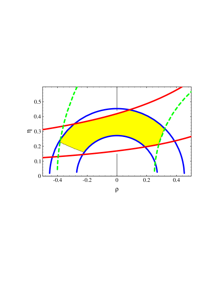
Figure 1: Range of allowed ($\eta$,$\rho$) values for $m_{t}^{\rm(pole)}$ = 169 GeV. See the text for explanations.

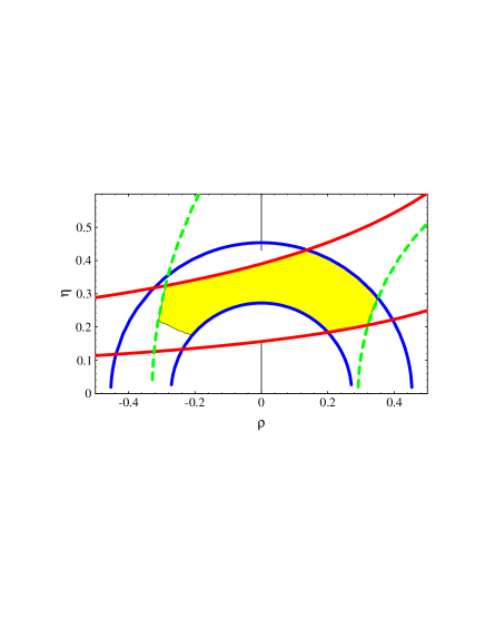
Figure 2: Same as in Fig. 1 for $m_{t}^{\rm(pole)}$ = 181 GeV.

Figs. 1 and 2 give the results of our analysis for the two extreme values of $m_{t}$: the area enclosed by the two black circumferences represents the constraint of eq. (54), the area between the two gray (dashed) circumferences is allowed by the bounds from eq. (55); the area enclosed by the two solid parabolic curves represents the solution of eq. (53) with the range of $\widehat{B}_{K}$ given in eq. (61) (notice that the upper parabolic curve corresponds to the minimal value of $V_{cb}$ and vice versa for the lower curve).

The gray region within the intersection of the curves is the range actually allowed after the correlation in $V_{cb}$ between eq. (53) and eq. (55) is taken into account. A further correlation is present when computing Im $\lambda_{t}$ from $\eta$ in eq. (63).

This procedure determines the allowed range for

$$\mathop{\mbox{Im}}\lambda_{t}\simeq\eta|V_{us}||V_{cb}|^{2}\,.$$ (63)

For a flat variation of the input parameters, including $\Lambda^{(4)}_{\rm QCD}$, we find

$$0.62\times 10^{-4}\leq\mathop{\mbox{Im}}\lambda_{t}\leq 1.4\times 10^{-4}\ .$$ (64)

For comparison, values of Im $\lambda_{t}$ between $0.86\times 10^{-4}$ and $1.7\times 10^{-4}$ are found in the most recent update of the Munich group [1] using $\widehat{B}_{K}=0.75\pm 0.15$. The larger values of $\widehat{B}_{K}$ we obtain reduce substantially the maximum values allowed for Im $\lambda_{t}$.

5 Estimating $\varepsilon^{\prime}/\varepsilon$ 

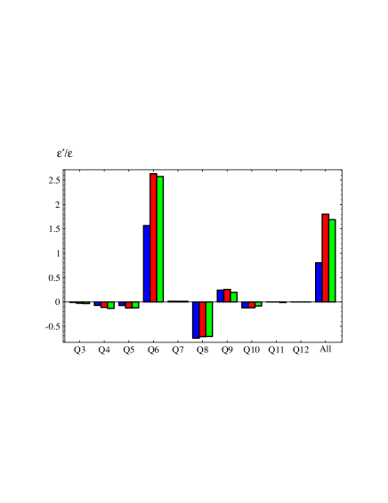
Figure 3: Anatomy of $\varepsilon^{\prime}/\varepsilon$ in units of $10^{-3}$ for central values of the input parameters: LO calculation (black), LO with chiral loops (half-tone), complete NLO result (gray). In the LO case we have taken $f=f_{\pi}$, whereas in the remaining hystograms the renormalized value $f=86$ MeV has been used.

We can now discuss our results for $\varepsilon^{\prime}/\varepsilon$ . Fig. 3 shows the impact on the final value of $\varepsilon^{\prime}/\varepsilon$ of each operator for the representative central values of all input parameters and $\mathop{\mbox{Im}}\lambda_{t}=1.0\times 10^{-4}$. The same figure also shows how the results vary from the LO predictions (black), once chiral loops (half-tone) and NLO (gray) corrections are included. The typical size of the $\chi$QM NLO corrections to the matrix elements of the quark operators is less than 10%.

The contribution of the chromomagnetic penguin $Q_{11}$ is very small for two reasons, as discussed in ref. [6]: its matrix element is vanishing at the LO, and the NLO result turns out to be proportional to $m_{\pi}^{2}$. Numerically, the matrix element of $Q_{11}$ is about 5% of the NLO corrections to the matrix element of $Q_{6}$.

The LO reduction of the contribution of the operator $Q_{8}$ caused by the $O(p^{2})$ correction terms is an important result of the present analysis. In fact, without them the contributions of $Q_{6}$ and $Q_{8}$ are at LO almost equal in absolute value thus leading to a vanishing value for $\varepsilon^{\prime}/\varepsilon$ . With the inclusion of the $O(p^{2})$ corrections the final value of $\varepsilon^{\prime}/\varepsilon$ turns out to be positive in the whole parameter range. It is important to remark that this result is also determined by the enhancement of the $Q_{6}$ matrix element due to the chiral loop corrections. In turn, this effect is related to the good fit of the amplitude $A_{0}(K^{0}\to\pi\pi)$ which we obtain in the same framework [7].

Figure 4: $\varepsilon^{\prime}/\varepsilon$ in units of $10^{-3}$ as a function of $\left\langle\bar{q}q\right\rangle$ ^1/3 (GeV) and $\lambda=$ Im $\lambda_{t}$ in units of $10^{-4}$, for central values of the other input parameters.

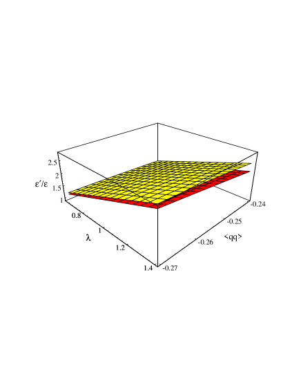
Figure 5: The dependence of $\varepsilon^{\prime}/\varepsilon$ in units of $10^{-3}$ on the matching scale $\mu$ as a function of $\left\langle\bar{q}q\right\rangle$ ^1/3 (GeV) and $\lambda=$ Im $\lambda_{t}$ in units of $10^{-4}$. The gray surface corresponds to $\mu=0.8$ GeV and the dark surface to $\mu=1$ GeV.

In order to understand the uncertainty in our estimate, we now present a detailed study of the determination of $\varepsilon^{\prime}/\varepsilon$ . The matrix elements depend on the values of the input parameters $\left\langle\bar{q}q\right\rangle$ and $\left\langle\alpha_{s}GG/\pi\right\rangle$ , besides that of the constituent quark mass $M$ characteristic of the $\chi$QM.

The range of values for $\left\langle\bar{q}q\right\rangle$ , $\left\langle\alpha_{s}GG/\pi\right\rangle$ and $M$ found in ref. [7] via the NLO best fit of the $\Delta I=1/2$ rule are reported in eqs. (18)–(20). Since the value of $\left\langle\alpha_{s}GG/\pi\right\rangle$ is not very important in the physics of penguin operators we can safely consider the central value of eq. (18) as a fixed input for our numerical analysis of $\varepsilon^{\prime}/\varepsilon$ .

A relevant parameter in determining the size of $\varepsilon^{\prime}/\varepsilon$ is $\mathop{\mbox{Im}}\lambda_{t}$, as discussed in the introduction. We use the overall range given by eq. (64).

Fig. 4 shows $\varepsilon^{\prime}/\varepsilon$ as a function of $\left\langle\bar{q}q\right\rangle$ and Im $\lambda_{t}$ for central values of the other input parameters. The stability of the result can be gauged by comparing the variation of the surface in Fig. 4 as we vary

• The matching scale $\mu$, between 0.8 and 1 GeV: Fig. 5;

• The values of $\Lambda_{\rm QCD}$ and $m_{t}$ in the ranges given in the appendix A: Fig. 6;

• The value of $M$ in the range of eq. (20): Fig. 7.

As we can see from Fig. 5, the dependence on the matching scale is very weak and vanishes within the range of $\left\langle\bar{q}q\right\rangle$ shown. We consider the scale stability a success of our approach.

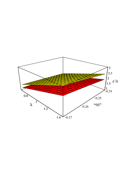
Figure 6: The dependence of $\varepsilon^{\prime}/\varepsilon$ (in units of $10^{-3}$) on $\Lambda_{\rm QCD}$ and $m_{t}$ as a function of $\left\langle\bar{q}q\right\rangle$ ^1/3 (GeV) and $\lambda=$ Im $\lambda_{t}$ in units of $10^{-4}$. The upper surface corresponds to $\Lambda^{(4)}_{\rm QCD}=380$ MeV and $m_{t}^{\rm(pole)}=169$ GeV while the lower surface corresponds to $\Lambda^{(4)}_{\rm QCD}=300$ MeV and $m_{t}^{\rm(pole)}=181$ GeV.

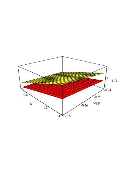
Figure 7: The dependence of $\varepsilon^{\prime}/\varepsilon$ in units of $10^{-3}$ on the constituent quark mass $M$ as a function of $\left\langle\bar{q}q\right\rangle$ ^1/3 (GeV) and $\lambda=$ Im $\lambda_{t}$ in units of $10^{-4}$. The upper surface corresponds to $M=197$ MeV, $\Lambda^{(4)}_{\rm QCD}=380$ MeV and $m_{t}^{\rm(pole)}=169$ GeV, while the lower surface corresponds to $M=205$ MeV, $\Lambda^{(4)}_{\rm QCD}=300$ MeV and $m_{t}^{\rm(pole)}=181$ GeV.

By varying $\Lambda_{\rm QCD}$, $m_{t}$, $\left\langle\bar{q}q\right\rangle$ and $\mathop{\mbox{Im}}\lambda_{t}$ in their respective ranges while keeping $M$ fixed at its central value, we find (Fig. 6)

$$\varepsilon^{\prime}/\varepsilon=1.7\ ^{+1.3}_{-0.9}\,\times\,10^{-3}\,.$$ (65)

The final source of uncertainty arises from the value of $M$. If we include its variation according to the range of eq. (20) we find (Fig. 7)

$$\varepsilon^{\prime}/\varepsilon=1.7\;^{+1.4}_{-1.0}\,\times\,10^{-3}\,.$$ (66)

The result in eq. (66) represents the most conservative estimate of the error in our prediction. The dependence on the remaining input parameter $m_{s}$ in the NLO corrections is small and can be safely neglected.

In comparing the present estimate with our previous one in ref. [3] (circa 1995), we may notice that the complete $O(p^{2})$ analysis of the bosonization of the operator $Q_{8}$ has reduced the impact of the electroweak corrections and accordingly $\varepsilon^{\prime}/\varepsilon$ is never negative. In addition, the inclusion in the present analysis of the effects of the rescattering phases, eqs. (8)–(9), enhances the $I=0$ channel, thus increasing the size of $\varepsilon^{\prime}/\varepsilon$ . As a consequence, the values of $\varepsilon^{\prime}/\varepsilon$ are now larger even though the NLO determination of the parameter $\widehat{B}_{K}=1.1\pm 0.2$ has made the maximum value of Im $\lambda_{t}$ roughly 30% smaller.

Finally, the updated new short-distance analysis, with the reduced range in $\Lambda^{(4)}_{\rm QCD}$, makes the whole estimate more stable.

5.1 Outlook

Our analysis, based on the implementation of the $\chi$QM and chiral lagrangian methods, takes advantage of the observation that the $\Delta I=1/2$ selection rule in kaon decays is well reproduced in terms of three basic parameters (the constituent quark mass $M$ and the quark and gluon condensates) in terms of which all hadronic matrix elements of the $\Delta S=1$ lagrangian can be expressed. We have used the best fit of the $\Delta I=1/2$ selection rule in kaon decays to constrain the allowed ranges of $M$, $\left\langle\bar{q}q\right\rangle$ and $\left\langle GG\right\rangle$ and have fed them in the analysis of $\varepsilon^{\prime}/\varepsilon$ based on the NLO $O(p^{4})$ determination of all hadronic matrix elements. Values of $\varepsilon^{\prime}/\varepsilon$ positive and of the order of $10^{-3}$ are preferred, even though values of $O(10^{-4})$ cannot be excluded.

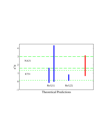
Figure 8: Present status of theoretical predictions and experimental values for $\varepsilon^{\prime}/\varepsilon$ (in units of $10^{-3}$). The two horizontal bands bounded by long- and short-dashed lines show the 1$\sigma$ experimental results of NA31 and E731 respectively. The vertical bars represent the theoretical predictions including the errors quoted by the authors. In gray we show our final estimate of eq. (66).

In Fig. 8 we have summarized the present status of the theoretical predictions for $\varepsilon^{\prime}/\varepsilon$. The two ranges we have reported for ref. [1] corresponds to taking two different determinations of $m_{s}$, namely, from left to right, $m_{s}(1.3\ {\rm GeV})=150\pm 20$ MeV and $m_{s}(1.3\ {\rm GeV})=100\pm 20$ MeV. The varying of $m_{s}$ in the approach of ref. [1] is the analogue of varying $\left\langle\bar{q}q\right\rangle$ in our LO matrix elements.

The smaller uncertainty in the lattice result [2] is due to the authors’ Gaussian treatment of the uncertainties in the input parameters, to be contrasted to a flat scanning. The results of ref. [1] as well as ours can be made proportionally smaller by a similar treatment of the errors.

Given the complexity of the computation, it is rewarding to find that so very different approaches lead to predictions that are reasonably in agreement with each other.

We would like to conclude by briefly discussing three issues that arise in comparing our present analysis with that of refs. [1] and [2]:

• The weight of the operator $Q_{4}$, that is negligible in our estimate (Fig. 3), is made sizable in those of refs. [1] and [2] by the assumption that the coefficient $B_{4}$ can be as large as 6. Such a large value comes from considering the relation

  $$Q_{4}=Q_{2}-Q_{1}+Q_{3}\ ,$$ (67)

  which is exact in the HV scheme, and the large value of the difference $\left\langle Q_{2}\right\rangle_{0}-\left\langle Q_{1}\right\rangle_{0}$ that is required in order to account for the $\Delta I=1/2$ rule. The $\chi$QM result of a negative $B_{3}$ shows that a large $\left\langle Q_{2}\right\rangle_{0}-\left\langle Q_{1}\right\rangle_{0}$ does not necessarily implies a correspondingly large value of $B_{4}$. A large value of $B_{4}$ makes $\varepsilon^{\prime}/\varepsilon$ smaller because the operator $Q_{4}$ gives a contribution of the opposite sign with respect to that of $Q_{6}$.

• In ref. [1] only the terms proportional to $G^{(0)}$ and $G^{b}_{LR}$ of the $\Delta S=1$ chiral lagrangian are included in the matrix elements of the operators $Q_{7,8}$. While the effect of the missing terms $G^{a,c}_{LR}$ is within the variation of the coefficient $B_{8}$ that is there considered, the central value of $\varepsilon^{\prime}/\varepsilon$ may be affected by such a choice.

• It is difficult to compare our approach to that of the lattice. We however notice that the contribution of the chiral term proportional to $G^{c}_{LR}$ only starts at the level of the $K\rightarrow 2\pi$ amplitude and therefore is not included when computing the two-point $K\rightarrow\pi$ transition, as currently done on the lattice. We would also like to stress the importance of always using the full $O(p^{2})$ $\Delta S=1$ chiral lagrangian (21) in computing the $K\rightarrow 2\pi$ from the $K\rightarrow\pi$ amplitude.

• Finally, the 20% enhancement of the $I=0$ amplitude due to the rescattering phase is included only in our analysis.

Appendix A Input Parameters

parameter	value
$\sin^{2}\theta_{W}(m_{Z})$	0.23
$m_{Z}$	91.187 GeV
$m_{W}$	80.33 GeV
$m_{t}^{\rm(pole)}$	$175\pm 6$ GeV
$m_{t}(m_{t})$	$167\pm 6$ GeV
$m_{t}(m_{W})$	$177\pm 7$ GeV
$m_{b}(m_{b})$	4.4 GeV
$m_{c}(m_{c})$	1.4 GeV
$m_{s}$ (1 GeV)	$178\pm 18$ MeV
$m_{u}+m_{d}$ (1 GeV)	$12\pm 2.5$ MeV
$\Lambda_{\rm QCD}^{(4)}$	$340\pm 40$ MeV
$V_{ud}$	0.9753
$V_{us}$	$0.2205\pm 0.0018$
$|V_{cb}|$	$0.040\pm 0.003$
$|V_{ub}/V_{cb}|$	$0.08\pm 0.02$
$\eta_{B}$	$0.55\pm 0.01$
$\sqrt{B_{B_{d}}}F_{B_{d}}$	$200\pm 40$ MeV
$\Delta M_{B_{d}}$	$0464\pm 0.018$ ps-1
$\widehat{B}_{K}$	$1.1\pm 0.2$
$\mathop{\mbox{Im}}\lambda_{t}$	$(1.0\pm 0.4)\times 10^{-4}$
$M$	$200\ ^{+5}_{-3}\>\mbox{MeV}$
$\left\langle\bar{q}q\right\rangle$	$-(240\ ^{+30}_{-10}\>\mbox{MeV})^{3}$
$\langle\alpha_{s}GG/\pi\rangle$	$(334\pm 4\>\mbox{MeV})^{4}$
$f$	86 $\pm$ 13 MeV
$f_{\pi}=f_{\pi^{+}}$	92.4 MeV
$f_{K}=f_{K^{+}}$	113 MeV
$m_{\pi}=(m_{\pi^{+}}+m_{\pi^{0}})/2$	138 MeV
$m_{K}=m_{K^{0}}$	498 MeV
$m_{\eta}$	548 MeV
$\Omega_{\eta+\eta^{\prime}}$	$0.25\pm 0.05$
$\cos\delta_{0}$	$0.8$
$\cos\delta_{2}$	$1.0$

Table 2: Table of the numerical values of the input parameters.

References

-
[1]
A.J. Buras, M. Jamin and M.E. Lautenbacher,
Phys. Lett. B 389 (1996) 749;
A.J. Buras and R. Fleischer, hep-ph/9704376 and references therein. -
[2]
M. Ciuchini, E. Franco, G. Martinelli and L. Reina, Phys. Lett. B 301 (1993) 263;
M. Ciuchini, E. Franco, G. Martinelli, L. Reina and L. Silvestrini, Z. Physik C 68 (1995) 239;
M. Ciuchini, hep-ph/9701278. - [3] S. Bertolini, J.O. Eeg and M. Fabbrichesi, Nucl. Phys. B 476 (1996) 225.
-
[4]
K. Nishijima, Nuovo Cim. 11 (1959) 698;
F. Gursey, Nuovo Cim. 16 (1960) 230 and Ann. Phys. (NY) 12 (1961) 91;
J.A. Cronin, Phys. Rev. 161 (1967) 1483;
S. Weinberg, Physica 96A (1979) 327;
A. Manohar and H. Georgi, Nucl. Phys. B 234 (1984) 189;
A. Manohar and G. Moore, Nucl. Phys. B 243 (1984) 55;
D. Espriu, E. de Rafael and J. Taron, Nucl. Phys. B 345 (1990) 22. -
[5]
J. Bijnens, C. Bruno and E. de Rafael, Nucl. Phys. B 390 (93) 501;
see, also: D. Ebert, H. Reinhardt and M.K. Volkov, in Prog. Part. Nucl. Phys. vol. 33, p. 1 (Pergamon, Oxford 1994);
J. Bijnens, Phys. Rep. 265 (1996) 369. -
[6]
S. Bertolini, M. Fabbrichesi and E. Gabrielli, Phys. Lett. B 327 (1994) 136;
S. Bertolini, J.O. Eeg and M. Fabbrichesi, Nucl. Phys. B 449 (1995) 197. - [7] S. Bertolini, J.O. Eeg, M. Fabbrichesi and E.I. Lashin, hep-ph/9705244.
- [8] G.D. Barr et al. (NA31 Coll.), Phys. Lett. B 317 (1993) 233.
- [9] L.K. Gibbons et al. (E731 Coll.),Phys. Rev. Lett. 70 (1993) 1203.
-
[10]
M.A. Shifman, A.I. Vainsthain and V.I. Zakharov,
Nucl. Phys. B 120 (1977) 316;
F.J. Gilman and M.B. Wise, Phys. Rev. D 20 (1979) 2392;
J. Bijnens and M.B. Wise, Phys. Lett. B 137 (1984) 245;
M. Lusignoli, Nucl. Phys. B 325 (1989) 33. -
[11]
A.J. Buras, M. Jamin, M.E. Lautenbacher and P.H. Weisz,
Nucl. Phys. B 370 (1992) 69, (Addendum) ibid. 375 (1992) 501; Nucl. Phys. B 400 (1993) 37;
A.J. Buras, M. Jamin and M.E. Lautenbacher, Nucl. Phys. B 400 (1993) 75; Nucl. Phys. B 408 (1993) 209;
M. Ciuchini, E. Franco, G. Martinelli and L. Reina, Nucl. Phys. B 415 (1994) 403; Phys. Lett. B 301 (1993) 263. - [12] V. Antonelli, S. Bertolini, J.O. Eeg, M. Fabbrichesi and E.I. Lashin, Nucl. Phys. B 469 (1996) 143.
- [13] A.E. Bergan and J.O. Eeg, Phys. Lett. B 390 (1997) 420.
-
[14]
S.M. Roy, Phys. Lett. B 36 (1971) 353;
J.-L. Basdevant, C.D. Froggatt and J.L. Petersen, Nucl. Phys. B 72 (1974) 413;
J.-L. Basdevant, P. Chapelle, C. Lopez and M. Sigelle, Nucl. Phys. B 98 (1975) 285;
C.D. Froggatt and J.L. Petersen, Nucl. Phys. B 129 (1977) 89. - [15] V. Antonelli, S. Bertolini, M. Fabbrichesi and E.I. Lashin, Nucl. Phys. B 469 (1996) 181.
- [16] A.J. Buras and J.M. Gerard, Phys. Lett. B 192 (1987) 156.
-
[17]
J.F. Donoghue et al., Phys. Lett. B 179 (1986) 361;
M. Lusignoli, Nucl. Phys. B 325 (1989) 33. - [18] J. Bijnens, Int. J. Mod. Phys. A 8 (1993) 3045.
- [19] M. Fabbrichesi and E.I. Lashin, Phys. Lett. B 387 (1997) 609.
- [20] M. Ciuchini, E. Franco, G. Martinelli and L. Reina, Estimates of , in The Second DANE Physics Handbook, eds. L. Maiani et al. (Frascati, 1995); Z. Physik C 68 (1995) 239 and references therein.
- [21] S.R. Sharpe, hep-lat/960929 and references therein.
- [22] A.J. Buras, M. Jamin and M.E. Lautenbacher, Nucl. Phys. B 408 (1993) 209
-
[23]
A.J. Buras, M. Jamin and P. H. Weisz, Nucl. Phys. B 347 (1990) 491;
S. Herrlich and U. Nierste, Nucl. Phys. B 419 (1994) 292; Phys. Rev. D 52 (1995) 6505; Nucl. Phys. B 476 (1996) 27. - [24] R.M. Barnett et al., Phys. Rev. D 54 (1996) 1 and 1997 off-year partial update for the 1998 edition available on the PDG WWW pages (URL: http://pdg.lbl.gov/).
- [25] V. Antonelli, S. Bertolini, M. Fabbrichesi and E.I. Lashin, Nucl. Phys. B 493 (1997) 281.
- [26] P.L. Tipton, in Proceedings of the 28th ICHEP (Warsaw), eds. Z. Ajduk and A.K. Wroblewski, page 123 (World Scientific, Singapore 1997).