QCD corrections to $b\rightarrow s\gamma\gamma$ induced decays:
$B\rightarrow X_{s}\gamma\gamma$ and $B_{s}\rightarrow\gamma\gamma$

Abstract

We present a complete calculation of the Leading Order QCD corrections to the quark level decay amplitude for $b\rightarrow s\gamma\gamma$ and study their relevance for both the inclusive branching ratio $BR(B\rightarrow X_{s}\gamma\gamma)$ and for the exclusive decay channel $B_{s}\rightarrow\gamma\gamma$. In addition to the uncertainties in the short distance calculation, due to the choice of the renormalization scale, an appreciable uncertainty in both $B_{s}\rightarrow\gamma\gamma$ and $B\rightarrow X_{s}\gamma\gamma$ is introduced by the matrix element calculation. We also briefly discuss some long distance effects, especially those due to the $\eta_{c}$ resonance for the inclusive rate. Finally, a brief analysis of the IR singularities of the two photon spectrum in the inclusive case is given.

1 Introduction

The radiative decays of the B meson are known to be very sensitive to strong interaction perturbative corrections as well as to the flavor structure of the electroweak interactions and to new physics beyond the Standard Model. In particular, both inclusive and exclusive processes induced by $b\rightarrow s\gamma$ have been studied in great detail [1, 2, 3, 4, 5] and two measurements already exist from the CLEO collaboration: $BR(B\rightarrow X_{s}\gamma)\!=\!(2.32\pm 0.57\pm 0.35)\times 10^{-4}$ and $BR(B\rightarrow K^{*}\gamma)\!=\!(4.2\pm 0.8\pm 0.6)\times 10^{-5}$.

Due to the impressive experimental effort which is being directed to the study of the physics of the B meson, we can be confident that much lower branching ratios will be measured in the future. Therefore it may be interesting to study processes induced at the quark level by a two photon radiative decay of the b quark, i.e. by $b\rightarrow s\gamma\gamma$.

The $b\rightarrow s\gamma\gamma$ decay has received some attention in the literature [6, 7, 8], because of the interest in the $B_{s}\rightarrow\gamma\gamma$ exclusive mode. More recently, in Ref. [9] we focused on the study of the inclusive $B\rightarrow X_{s}\gamma\gamma$ branching ratio. In the pure electroweak theory, without QCD corrections but after the necessary kinematical cuts to isolate the contribution into hard photons are imposed, both branching ratios are found to be of order $10^{-7}$. There is at present an experimental upper bound on the $BR(B_{s}\rightarrow\gamma\gamma)$, namely $BR(B_{s}\rightarrow\gamma\gamma)<1.48\times 10^{-4}$ [10].

As we know from the study of $b\rightarrow s\gamma$, the impact of QCD corrections on radiative B decays can be pretty dramatic. Therefore in this sequel, as we promised in [9], we now want to present the study of Leading Order QCD corrections to the quark level process $b\rightarrow s\gamma\gamma$. We will use this result to predict the QCD corrected branching ratios for both the inclusive $B\rightarrow X_{s}\gamma\gamma$ and the exclusive $B_{s}\rightarrow\gamma\gamma$ mode. In both cases QCD corrections increase the branching ratio by $60\%$ to more than $100\%$. On the other hand, the forward-backward asymmetry that was introduced in [9] turns out to be very robust with respect to QCD corrections and always varies by less than $15\%$.

In order to motivate the interest of our perturbative calculation we will also comment about some relevant long distance contributions and devote particular attention to the effect of the $\eta_{c}$ resonance in the inclusive case. Moreover, we will see how some uncertainty for both the inclusive and the exclusive branching ratio is introduced at the level of the matrix element calculation, due to the dependence on $m_{s}$.

Finally, we will give in Appendix A the detailed description of the treatment of the IR singularities which arise in the spectrum of the two photons for $B\rightarrow X_{s}\gamma\gamma$.

2 Leading Order QCD corrections to $b\rightarrow s\gamma\gamma$.

In this section we present the general structure of the leading Order QCD corrections to the quark level decay process $b\rightarrow s\gamma\gamma$. We will give the expression for the amplitude $A(b\rightarrow s\gamma\gamma)$, including a complete resummation of the leading QCD corrections to all orders in $(\alpha_{s}\log(\mu^{2}/M_{W}^{2}))^{n}$. The result will be then specialized in the following sections to the calculation of the inclusive branching ratio $BR(B\rightarrow X_{s}\gamma\gamma)$ and of the exclusive branching ratio for the decay $B_{s}\rightarrow\gamma\gamma$.

We will discuss QCD corrections in the well established framework of electroweak effective hamiltonians with renormalization group improved resummation of QCD corrections. For a complete review of the subject see Ref. [11]. The most general effective hamiltonian which describes radiative $b\rightarrow s$ decays with up to three emitted gluons or photons is given by [12, 13]

$$H_{eff}=-\frac{4G_{F}}{\sqrt{2}}V_{tb}V_{ts}^{*}\sum_{i=1}^{8}C_{i}(\mu)O_{i}\,\,\,,$$ (1)

where, as usual, $G_{F}$ denotes the Fermi coupling constant and $V_{ij}$ indicates some Cabibbo-Kobayashi-Maskawa (CKM) matrix element. In writing Eq. (1), we have used the unitarity of the CKM matrix and we have taken into account that for $b\rightarrow s$ transitions $V_{ub}V_{us}^{*}\ll V_{tb}V_{ts}^{*}\simeq V_{cb}V_{cs}^{*}$. The basis of local operators we use is obtained from the more general set of gauge invariant dimension five and six local operators with up to three external gauge bosons by appling the QED and QCD equations of motion [12, 13] and is expressed in terms of the following operators

$$O_{1} = (\bar{s}_{\alpha}\gamma^{\mu}Lc_{\beta})(\bar{c}_{\beta}\gamma_{\mu}Lb_{\alpha})\,\,\,,$$

$$O_{2} = (\bar{s}_{\alpha}\gamma^{\mu}Lc_{\alpha})(\bar{c}_{\beta}\gamma_{\mu}Lb_{\beta})\,\,\,,$$

$$O_{3,5} = (\bar{s}_{\alpha}\gamma^{\mu}Lb_{\alpha})\sum_{q=u,\ldots,b}(\bar{q}_{\beta}\gamma_{\mu}(L,R)q_{\beta})\,\,\,,$$ (2)

$$O_{4,6} = (\bar{s}_{\alpha}\gamma^{\mu}Lb_{\beta})\sum_{q=u,\ldots,b}(\bar{q}_{\beta}\gamma_{\mu}(L,R)q_{\alpha})\,\,\,,$$

$$O_{7} = \frac{e}{16\pi^{2}}\bar{s}_{\alpha}\sigma^{\mu\nu}(m_{b}R+m_{s}L)b_{\alpha}F_{\mu\nu}\,\,\,,$$

$$O_{8} = \frac{g_{s}}{16\pi^{2}}\bar{s}_{\alpha}\sigma^{\mu\nu}(m_{b}R+m_{s}L)t^{a}_{\alpha\beta}b_{\beta}G^{a}_{\mu\nu}\,\,\,,$$

where the chiral structure is specified by the projectors $L,R=(1\mp\gamma_{5})/2$, while $\alpha$ and $\beta$ are color indices. $F_{\mu\nu}$ and $G_{\mu\nu}^{a}$ denotes the QED and QCD field strength tensors respectively, also $e$ and $g_{s}$ stand for the electromagnetic and strong coupling constants.

The Wilson coefficients $C_{i}(\mu)$ are process independent and their renormalization is determined only by the basis of operators $\{O_{i}\}$. They depend on the renormalization scale $\mu$ which we will set eventually to $\mu\approx m_{b}$. This introduces an error in the theory that is quite significant when only Leading Order (LO) logarithms of the form $(\alpha_{s}\log(\mu^{2}/M_{W}^{2}))^{n}$ are taken into account and gets appreciably reduced when also Next-to-Leading Order (NLO) logarithms of the form $\alpha_{s}(\alpha_{s}\log(\mu^{2}/M_{W}^{2}))^{n}$ are resummed. The LO result for the Wilson coefficients in Eq. (1) is now a well established result [1] and recently the authors of Ref. [2] provided us with the first NLO calculation.

If we want to calculate the amplitude for $b\rightarrow s\gamma\gamma$ at LO we have to use the effective hamiltonian in Eq. (1) with LO Wilson coefficients and evaluate its matrix element for the $b\rightarrow s\gamma\gamma$ decay at $O(\alpha_{s}^{0})$. On the other hand, for a NLO result we have to use NLO Wilson coefficients and include $O(\alpha_{s})$ corrections to the matrix element.

In order to understand the impact of QCD corrections on this new class of rare radiative B-decays, we choose to perform our analysis including, for the time being, only LO corrections. Therefore we will take the LO regularization scheme independent Wilson coefficients from the literature [3] and will not consider explicitly the matrix elements due to the insertion of $O_{5}$ and $O_{6}$ into the one photon and one gluon penguin diagrams. In fact these matrix elements are reabsorbed into the scheme independent definition of $C_{7}(\mu)$ and $C_{8}(\mu)$

$$C_{7,8}^{\rm eff}(\mu)=C_{7,8}(\mu)+\vec{Z}_{7,8}^{T}\cdot\vec{C}(\mu)\,\,\,,$$ (3)

where $\vec{C}(\mu)$ is the vector of $C_{1}(\mu),\ldots,C_{6}(\mu)$, while the vectors $\vec{Z}_{7,8}$ depend on the regularization scheme: they are zero in the ’t Hooft-Veltman (HV) scheme and non zero in the Naïve Dimensional Reduction scheme (NDR) (see Ref. [3] for details). In our calculation, we use the $C_{i}^{\rm eff}$ effective coefficients, although we decide to drop the extra index to simplify the notation. We note that no new regularization scheme dependence enters in the calculation of the matrix elements for $b\rightarrow s\gamma\gamma$ through the new class of penguin diagrams with two external photons. In fact, a finite scheme dependence in the matrix element can arise only as a result of the product of the UV pole part of a Feynman diagram (or set of diagrams) times some $O(\epsilon)$ evanescent Dirac structure of the diagram itself. However, as we will see, the new penguins with two external photons are UV finite at $O(\alpha_{s}^{0})$. Therefore any difference between two regularization schemes can only give an unphysical $O(\epsilon)$ effect. We have performed the calculation of the following matrix elements in both the HV and NDR regularization schemes and, as expected, the results coincide. Therefore we do not specify any regularization scheme in the following discussion.

The amplitude for the decay $b(p)\rightarrow s(p^{\prime})+\gamma(k_{1})+\gamma(k_{2})$ can be expressed as

$$A=\sum_{i=1}^{7}A_{i}=-\frac{ie^{2}G_{F}}{\sqrt{2}\pi^{2}}\lambda_{t}\sum_{i=1}^{7}C_{i}(\mu)\bar{u}_{s}(p^{\prime})T_{i}^{\mu\nu}u_{b}(p)\epsilon_{\mu}(k_{1})\epsilon_{\nu}(k_{2})\,\,\,,$$ (4)

where $\lambda_{t}=V_{tb}V_{ts}^{*}$ and $\epsilon_{\mu}(k_{1})$ and $\epsilon_{\nu}(k_{2})$ are the polarization vectors of the two photons. The $C_{i}(\mu)$ coefficient are intended to be the LO ones, as explained before, while we have denoted by $T_{i}^{\mu\nu}$ the tensor structure of the transition amplitude induced by the operator $O_{i}$. The different $T_{i}^{\mu\nu}$ are obtained inserting the operators of Eq. (2) into the Feynman diagrams of Fig. 1, according to the color and chiral structure of the operators themselves.

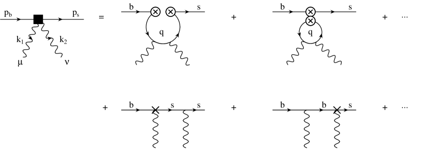
Figure 1: Examples of Feynman diagrams which contribute to the matrix element $\langle s\gamma\gamma|H_{\mathrm{eff}}|b\rangle$. The 1PI diagrams illustrate the two possible insertions of the operators $O_{1},\dots,O_{6}$ (double circled cross vertices), depending on their flavor, chiral and color structure, while the 1PR ones represent the insertion of $O_{7}$ (cross vertices). Moreover q indicates a generic quark flavor.

In particular, one has to be careful when dealing with penguin-like operators $O_{3,\ldots,6}$ due to their more complicated flavor structure. The $T_{i}^{\mu\nu}$ tensors can be summarized in a compact form as follows

$$T_{1}^{\mu\nu} = N_{c}Q_{u}^{2}\kappa_{c}W_{2}^{\mu\nu}\,\,\,,$$

$$T_{2}^{\mu\nu} = Q_{u}^{2}\kappa_{c}W_{2}^{\mu\nu}\,\,\,,$$

$$T_{3}^{\mu\nu} = \left\{N_{c}\left[Q_{d}^{2}\left(\kappa_{d}+\kappa_{s}+\kappa_{b}\right)+Q_{u}^{2}\left(\kappa_{u}+\kappa_{c}\right)\right]+Q_{d}^{2}\left(\kappa_{b}+\kappa_{s}\right)\right\}W_{2}^{\mu\nu}\,\,\,,$$

$$T_{4}^{\mu\nu} = \left\{\left[Q_{d}^{2}\left(\kappa_{d}+\kappa_{s}+\kappa_{b}\right)+Q_{u}^{2}\left(\kappa_{u}+\kappa_{c}\right)\right]+N_{c}Q_{d}^{2}\left(\kappa_{s}+\kappa_{b}\right)\right\}W_{2}^{\mu\nu}\,\,\,,$$ (5)

$$T_{5}^{\mu\nu} = -N_{c}\left[Q_{d}^{2}\left(\kappa_{d}+\kappa_{s}+\kappa_{b}\right)+Q_{u}^{2}\left(\kappa_{u}+\kappa_{c}\right)\right]W_{2}^{\mu\nu}+Q_{d}^{2}\left[m_{b}W_{5,b}^{\mu\nu}R+m_{s}W_{5,s}^{\mu\nu}L\right]\,\,\,,$$

$$T_{6}^{\mu\nu} = -\left[Q_{d}^{2}\left(\kappa_{d}+\kappa_{s}+\kappa_{b}\right)+Q_{u}^{2}\left(\kappa_{u}+\kappa_{c}\right)\right]W_{2}^{\mu\nu}+N_{c}Q_{d}^{2}\left[m_{b}W_{5,b}^{\mu\nu}R+m_{s}W_{5,s}^{\mu\nu}L\right]\,\,\,,$$

$$T_{7}^{\mu\nu} = Q_{d}W_{7}^{\mu\nu}\,\,\,,$$

where we note that there is no contribution from the chromo-magnetic operator $O_{8}$ at $O(\alpha_{s}^{0})$. In Eq. (2) $N_{c}$ denotes the number of colors ($N_{c}\!=\!3$), $Q_{u}\!=\!2/3$ and $Q_{d}\!=\!-1/3$ are the up-type and down-type quark electric charges and $m_{b}$ and $m_{s}$ indicate the masses of the bottom and of the strange quark respectively. Moreover all the $T_{i}^{\mu\nu}$ have been expressed in terms of only three tensor structures

$$W_{2}^{\mu\nu} = \left\{\frac{1}{k_{1}\cdot k_{2}}\left[k_{1}^{\nu}k_{1}\!\!\!\!/\gamma^{\mu}k_{2}\!\!\!\!/-k_{2}^{\mu}k_{1}\!\!\!\!/\gamma^{\nu}k_{2}\!\!\!\!/-k_{2}^{\mu}k_{1}^{\nu}\left(k_{1}\!\!\!\!/-k_{2}\!\!\!\!/\right)\right]+\right.$$ (6)

$$\,\,\,\,\,\,\,\,\,\left.\phantom{\frac{1}{k_{1}\cdot k_{2}}}\gamma^{\nu}\gamma^{\mu}\left(k_{1}\!\!\!\!/-k_{2}\!\!\!\!/\right)-g^{\mu\nu}\left(k_{1}\!\!\!\!/-k_{2}\!\!\!\!/\right)+2k_{1}^{\nu}\gamma^{\mu}\right\}L\,\,\,,$$

$$W_{5,q}^{\mu\nu} = \frac{1}{m_{q}^{2}}\left(\gamma^{\nu}k_{2}\!\!\!\!/\gamma^{\mu}k_{1}\!\!\!\!/+k_{1}\cdot k_{2}\gamma^{\nu}\gamma^{\mu}+g^{\mu\nu}k_{2}\!\!\!\!/\,k_{1}\!\!\!\!/-k_{2}^{\mu}\gamma^{\nu}k_{1}\!\!\!\!/-k_{1}^{\nu}k_{2}\!\!\!\!/\gamma^{\mu}\right)\left(1-2\kappa_{q}\right)+$$

$$\,\,\,\,\,\,\,\,\,4\left(g^{\mu\nu}-\frac{k_{1}^{\nu}k_{2}^{\mu}}{k_{1}\cdot k_{2}}\right)\kappa_{q}\,\,\,,$$

$$W_{7}^{\mu\nu} = \frac{1}{2}\left[-\frac{1}{2p\cdot k_{2}}k_{1}\!\!\!\!/\gamma^{\mu}(m_{b}R+m_{s}L)(p\!\!\!/-k_{2}\!\!\!\!/+m_{b})\gamma^{\nu}+\right.$$

$$\,\,\,\,\,\,\,\left.\frac{1}{2p^{\prime}\cdot k_{2}}\gamma^{\nu}(p\!\!\!/-k_{1}\!\!\!\!/+m_{s})k_{1}\!\!\!\!/\gamma^{\mu}(m_{b}R+m_{s}L)\right]\,+\,\left(\{k_{1},\mu\}\leftrightarrow\{k_{2},\nu\}\right)\,\,\,,$$

and the analytic coefficients $\kappa_{q}$ defined as

$$\kappa_{q}=\frac{1}{2}+\frac{Q_{0}(z_{q})}{z_{q}}=\frac{1}{2}+\frac{1}{z_{q}}\int_{0}^{1}\frac{dx}{x}\log(1-z_{q}x+z_{q}x^{2})\,\,\,,$$ (7)

for $z_{q}\!=\!2k_{1}\cdot k_{2}/m_{q}^{2}\,\,$. In derivng Eq. (2)-(7) we have checked the analogous results given in Refs. [15, 14] for the $b\rightarrow s\gamma g$ decay and we confirm all of them.

Finally, we observe that using the effective hamiltonian of Eq. (1) at $\mu\simeq M_{W}$ and in the absence of QCD corrections, we can reproduce the pure electroweak amplitude obtained in Refs. [6, 7, 8], as expected. Only two operators, $O_{2}$ and $O_{7}$, contribute in this case. Their Wilson coeffcients at $\mu\!=\!M_{W}$ read

$$C_{2}(M_{W}) = 1\,\,\,,$$

$$C_{7}(M_{W}) = F_{2}(x_{t})-F_{2}(x_{c})\,\,\,,$$ (8)

where $F_{2}(x_{i})$ is the Inami-Lim function for the on-shell $bs\gamma$ vertex [16]

$$F_{2}(x_{i})=\frac{3x_{i}^{3}-2x_{i}^{2}}{4(x_{i}-1)^{4}}\log x_{i}+\frac{-8x_{i}^{3}-5x_{i}^{2}+7x_{i}}{24(x_{i}-1)^{3}}\,\,\,.$$ (9)

The corresponding matrix elements are given in Eq. (2) and we can easily verify that $O_{2}$ reproduces the one particle irreducible part of the result of Refs. [6, 7, 8] while $O_{7}$ is responsible for the one particle reducible part.

3 Inclusive branching ratio for $b\rightarrow s\gamma\gamma$.

As already discussed in Ref. [9], the inclusive rate for $B\rightarrow X_{s}\gamma\gamma$ can be described to a good degree of accuracy by the quark level process. We can therefore directly use the results of Section 2 to evaluate the square amplitude. For this purpose, we rewrite the amplitude as

$$A=-\frac{ie^{2}G_{F}}{\sqrt{2}\pi^{2}}\lambda_{t}\bar{u}_{s}(p^{\prime})\left[F_{2}W_{2}^{\mu\nu}+F_{5}\left(m_{b}W_{5,b}^{\mu\nu}R+m_{s}W_{5,s}^{\mu\nu}L\right)+F_{7}W_{7}^{\mu\nu}\right]u_{b}(p)\epsilon_{\mu}(k_{1})\epsilon_{\nu}(k_{2})\,\,\,,$$ (10)

where the coefficients $F_{i}$ can be easily deduced from Eqs. (4)-(2), and are

$$F_{2} = (N_{c}C_{1}(\mu)+C_{2}(\mu))Q_{u}^{2}\kappa_{c}+$$ (11)

$$C_{3}(\mu)\left\{N_{c}\left[Q_{d}^{2}(\kappa_{d}+\kappa_{s}+\kappa_{b})+Q_{u}^{2}\left(\kappa_{u}+\kappa_{c}\right)\right]+Q_{d}^{2}(\kappa_{s}+\kappa_{b})\right\}+$$

$$C_{4}(\mu)\left\{\left[Q_{d}^{2}(\kappa_{d}+\kappa_{s}+\kappa_{b})+Q_{u}^{2}\left(\kappa_{u}+\kappa_{c}\right)\right]+N_{c}Q_{d}^{2}\left(\kappa_{s}+\kappa_{b}\right)\right\}-$$

$$(N_{c}C_{5}(\mu)+C_{6}(\mu))\left[Q_{d}^{2}(\kappa_{d}+\kappa_{s}+\kappa_{b})+Q_{u}^{2}\left(\kappa_{u}+\kappa_{c}\right)\right]\,\,\,,$$

$$F_{5} = (C_{5}(\mu)+N_{c}C_{6}(\mu))Q_{d}^{2}\,\,\,,$$

$$F_{7} = C_{7}(\mu)Q_{d}\,\,\,.$$

The square amplitude summed over spins and polarizations will then be given by

$$|A|^{2} = \frac{1}{4}\left(\frac{e^{2}G_{F}}{\sqrt{2}\pi^{2}}\lambda_{t}\right)^{2}m_{b}^{4}\left[|F_{2}|^{2}A_{22}+|F_{5}|^{2}A_{55}+|F_{7}|^{2}A_{77}+2\mbox{Re}(F_{7}F_{2}^{*})A_{27}+\right.$$

$$\left.2\mbox{Re}(F_{5}F_{2}^{*}(1-2\kappa_{b}))A_{25}^{b}+2\mbox{Re}(F_{5}F_{2}^{*}(1-2\kappa_{s}))A_{25}^{s}+2\mbox{Re}(F_{7}F_{5}^{*})A_{57}\right]\,\,\,,$$

where the quantities $A_{ij}$ denote the contractions between the tensors $W_{i}^{\mu\nu}$ and $W_{j}^{\mu\nu}$. In order to give them explicitily we introduce the following notation

$$s=\frac{2k_{1}\cdot k_{2}}{m_{b}^{2}}\,\,\,\,,\,\,\,\,t=\frac{2p\cdot k_{2}}{m_{b}^{2}}\,\,\,\,,\,\,\,\,u=\frac{2p\cdot k_{1}}{m_{b}^{2}}\,\,\,\,,\,\,\,\,\rho=\frac{m_{s}^{2}}{m_{b}^{2}}\,\,\,,$$ (13)

which satisfy the relation: $u+t-s=1-\rho$. In order to introduce a more compact notation, it can be useful to switch occasionaly to the ($\bar{s}$, $\bar{u}$, $\bar{t}$) invariants, defined as $\bar{s}\!=\!s/(1-\rho)$, $\bar{t}\!=\!t/(1-\rho)$ and $\bar{u}\!=\!u/(1-\rho)$. In this framework the $A_{ij}$ quantities are given by:

$$A_{22} = 2\left[(1-\rho)^{2}-(1+\rho)s\right]\,\,\,,$$

$$A_{55} = \left[16|\kappa_{b}|^{2}+|(1-2\kappa_{b})s+4\kappa_{b}|^{2}+\rho\left(16|\kappa_{s}|^{2}+|(1-2\kappa_{s})s/\rho+4\kappa_{s}|^{2}\right)\right](1-s+\rho)+$$

$$16\,\mbox{Re}\left\{8\rho\kappa_{b}\kappa_{s}^{*}+s\left[\kappa_{b}-2(1+\rho)\kappa_{b}\kappa_{s}^{*}+\rho\kappa_{s}^{*}\right]\right\}\,\,\,,$$

$$A_{25}^{b,s} = \pm s(1-\rho\mp s)\,\,\,,$$ (14)

$$A_{27} = -2\left[(1+\rho)s+\frac{\rho s^{2}}{(s-t)t}+\frac{\rho s^{2}}{(s-u)u}\right]\,\,\,,$$

$$A_{57} = \mbox{Re}\left\{\phantom{\frac{1}{2}}8(\kappa_{b}+\rho\kappa_{s})s-\left[4\rho(\kappa_{b}+\kappa_{s})+s\left((1-2\kappa_{s})+\rho(1-2\kappa_{b})\right)\right]\right.$$

$$\left.\left[\frac{s^{2}}{t(s-t)}+\frac{s^{2}}{u(s-u)}\right]\right\}\,\,\,,$$

$$A_{77} = (1+\rho)\left[(1-\rho)A_{77}^{(1)}-2A_{77}^{(2)}\right]+A_{77}^{(3)}\,\,\,,$$

with

$$A_{77}^{(1)} = \frac{1}{\bar{t}}\left[1+\bar{u}+\frac{2\bar{u}(\bar{u}-2)}{1-\bar{u}}\bar{t}+\frac{2\bar{u}-1}{1-\bar{u}}\bar{t}^{2}\right]+(\bar{t}\leftrightarrow\bar{u})\,\,\,,$$

$$A_{77}^{(2)} = \frac{1}{\bar{t}^{2}}\left[1-\frac{1+\rho}{1-\bar{u}}\bar{t}+\frac{\rho}{(1-\bar{u})^{2}}\bar{t}^{2}\right]+(\bar{t}\leftrightarrow\bar{u})\,\,\,,$$ (15)

$$A_{77}^{(3)} = -2\frac{s}{\bar{t}\bar{u}}\left\{(1+\rho)(2+\bar{u}\bar{t})+\frac{\rho}{1-\rho}\left[1-\frac{2(1+\rho)-\bar{t}\bar{u}}{(1-\bar{t})(1-\bar{u})}\right]\bar{s}\right\}\,\,\,.$$

We want to put particular emphasis on the structure of the $A_{77}$ part of the square amplitude because it will be a crucial ingredient in testing the cancellation of the IR divergences which appear in the calculation of the total rate. In fact, the total rate is obtained by integrating

$$d\Gamma=\frac{1}{2m_{b}(2\pi)^{2D-3}}\delta^{D}(p-p^{\prime}-k_{1}-k_{2})|A|^{2}\frac{d^{(D-1)}p^{\prime}}{2p^{\prime}_{0}}\frac{d^{(D-1)}k_{1}}{2\omega_{1}}\frac{d^{(D-1)}k_{2}}{2\omega_{2}}\,\,\,,$$ (16)

over the physical phase space, where we have denoted by $\omega_{1}$ and $\omega_{2}$ the energies of the two photons. All the terms in $|A|^{2}$ are both UV and IR finite except $A_{77}$ which gives origin to IR singularities upon integration over the phase space of the two photons. We chose to regularize the integrals working in $D=4-2\epsilon$ dimensions and to extract the existing IR singularities as poles in $1/\epsilon$. These IR divergences originate when either $\omega_{1}\rightarrow 0$ or $\omega_{2}\rightarrow 0$, and correspond to the well known IR singularities which arise in the bremstrahlung process when one or the other of the two photons becomes very soft. In this limit the $b\rightarrow s\gamma\gamma$ decay cannot be distinguished from $b\rightarrow s\gamma$ and the two processes have to be considered together in order to obtain meaningful (i.e., finite) physical quantities. In fact, we have checked that the IR singularities which arise from the integration of $A_{77}$ over the phase space cancel exactly with the $O(\alpha_{e})$ virtual corrections to the $b\rightarrow s\gamma$ amplitude (see Appendix A). Therefore $(\Gamma(b\rightarrow s\gamma)+\Gamma(b\rightarrow s\gamma\gamma))$ is free of IR singularities.

This problem has already been studied in detail in order to take into account the $O(\alpha_{s})$ bremstrahlung corrections for $b\rightarrow s\gamma$ [15, 14]. However our point of view here is slightly different. In our case the bremstrahlung process is not considered as an $O(\alpha_{e})$ correction to the $b\rightarrow s\gamma$ amplitude, but as a different process: the decay of a $b$ quark into an $s$ quark plus two hard photons. Therefore, the endpoints of the spectrum of each photon (where the IR singularities are present) do not in fact correspond to the process of interest. In order to calculate the physical rate of interest we just have to impose a cut on the energy of each photon, which will naturally correspond to the experimental cut imposed on the minimun energy for detectable photons.

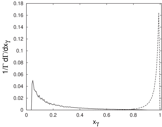
Figure 2: The spectrum of the two photons including QCD corrections, normalized to the total QCD corrected rate for $m_{s}\!=\!0.5$ GeV. The two photons are defined as the photon of lower energy (solid) and the photon of higher energy (dashed).

In Fig. 2 we illustrate the spectrum of the two photons, defined as the photon of higher energy and the photon of lower energy. We obtain this spectrum requiring the energy of each photon to be larger than $E_{\gamma}^{\rm min}\!=\!100$ MeV and the angles between any two outgoing particles to be bigger than $\theta_{ij}^{\rm min}\!=\!20^{\circ}$. This last constraint is not required analytically, but we think it is reasonable to exclude photons which are emitted too close to each other or to the outgoing s quark, in order to roughly incorporate the experimental requirements as we perceive them. Once the structure of the differential rate has been checked and the presence of IR singularities understood and treated, we can integrate Eq. (16) numerically and study the impact of QCD corrections on the total rate as well as on different distributions.

We find that QCD corrections enhance the rate by a factor of $\simeq 2-2.5$, depending on the numerical parameters we use. In our evaluation we fix $m_{b}\!=\!4.8$ GeV, $m_{c}\!=\!1.5$ GeV, $m_{t}\!=\!175$ GeV and $|\lambda_{t}|\!=\!|V_{tb}V_{ts}^{*}|\!=\!0.04$. As far as $m_{s}$ is concerned, we use $m_{s}\!\simeq\!M_{K}\!=\!0.5$ GeV. For this set of parameters and fixing $\mu\!=\!m_{b}$, the branching ratio for $B\rightarrow X_{s}\gamma\gamma$ goes from $\sim 1.7\times 10^{-7}$, without QCD corrections, to $\sim 3.7\times 10^{-7}$ when LO QCD corrections are included. We recall that we define the $BR(B\rightarrow X_{s}\gamma\gamma)$ in terms of the semileptonic branching ratio as follows

$$BR(B\rightarrow X_{s}\gamma\gamma)\simeq\left[\frac{\Gamma(b\rightarrow s\gamma\gamma)}{\Gamma(b\rightarrow cl\nu_{l})}\right]^{\mathrm{th}}\times BR(B\rightarrow X_{c}l\nu_{l})^{\mathrm{exp}}\,\,\,,$$ (17)

where no QCD corrections have to be included in the theoretical prediction of $\Gamma(b\rightarrow cl\nu_{l})$ at this order in $\alpha_{s}$ and we have used $BR(B\rightarrow X_{c}l\nu_{l})\simeq 0.11$ [17].

In principle, $m_{s}\!\simeq M_{K}$ should be used in the phase space integration, while in the perturbative calculation of the amplitude one may need to replace it by the current mass $m_{s}\!\simeq\!0.15$ GeV. However this introduces spurious instabilities in the numerical Montecarlo integration over the phase space. Since the numerical results change little as we replace $m_{s}$ over the range $0.15\!-\!0.5$ GeV, we prefer to use the same value of $m_{s}$ in both cases. Thus, in order to simulate the physical phase space correctly we set $m_{s}\!\simeq\!M_{K}$ everywhere.

Moreover, we have to account for the scale dependence introduced by QCD corrections at the level of the Wilson coefficients. This makes a $25-30\%$ uncertainty, as is the case for $B\rightarrow X_{s}\gamma$ case. For the sake of completion, we also give the values of the Wilson coefficients we use in Table 1, for three values of $\mu$, $\mu\!=\!m_{b}/2$, $m_{b}$ and $2m_{b}$ respectively, and for $m_{t}\!=\!175$ GeV and $\alpha_{s}(M_{W})\!=\!0.118$. We will comment about further uncertainties introduced by long distance QCD effects in Section 5.

$\mu$	$C_{1}$	$C_{2}$	$C_{3}$	$C_{4}$	$C_{5}$	$C_{6}$	$C_{7}$
$m_{b}/2$	-0.324	1.148	0.015	-0.033	0.009	-0.043	-0.344
$m_{b}$	-0.234	1.100	0.010	-0.024	0.007	-0.029	-0.308
$2m_{b}$	-0.162	1.065	0.007	-0.017	0.005	-0.019	-0.277

Table 1: Values of the regularization scheme independent LO Wilson coefficients for $\mu\!=m_{b}/2$, $\mu\!=m_{b}$, and $\mu\!=2m_{b}$, for $m_{b}\!=\!4.8$ GeV, $m_{t}\!=\!175$ GeV and $\alpha_{s}(M_{W})\!=\!0.118$.

In order to better understand the dynamics of QCD corrections, let us classify the different contributions to the rate into one particle reducible (1PR) and one particle irreducible (1PI), as we did in Ref. [9] for the pure electroweak case. In the language of the effective hamiltonian of Eq. (1) this corresponds to separating the cotribution of $O_{7}$ (which corresponds to the IPR part) from that of all the other operators. As we saw [9], the photon invariant mass distribution, $d\Gamma/ds$ is dominated for low $s$ by the 1PR diagrams, while for larger $s$ a non trivial $m_{c}$-dependent contribution from the 1PI diagrams starts being relevant. The effect of QCD corrections is to enhance even more the effect of $O_{7}$, as we could expect from the dramatic effect that QCD corrections have in $b\rightarrow s\gamma$, while lowering the impact of the 1PI contribution, because of the new mixing with many different four-quark operators. In particular, the contribution of $O_{2}$ is suppressed by the destructive interference with $O_{1}$. We verified that the contributions of different operators to the angular distribution of the two photons are very similar to each other, also after QCD corrections have been included.

On the other hand, as expected, the forward-backward asymmetry we introduced in [9]

$$A_{\mathrm{FB}}=\frac{\Gamma(\cos\theta_{s\gamma}\geq 0)-\Gamma(\cos\theta_{s\gamma}<0)}{\Gamma(\cos\theta_{s\gamma}\geq 0)+\Gamma(\cos\theta_{s\gamma}<0)}\,\,\,\,,$$ (18)

where $\theta_{s\gamma}$ is the angle between the s quark and the softer photon, is rather insensitive to QCD corrections, since the QCD corrections tend to cancel between the numerator and the denominator. In fact we find that QCD corrections affect $A_{\mathrm{FB}}$ by no more than $15\%$, changing it from 0.71 (without QCD corrections) to 0.78 (with LO QCD corrections), despite the fact that the total rate changes by as much as $60\%$ to $100\%$. Furthermore $A_{\mathrm{FB}}$ is practically insensitive to the choice of scale in the LO Wilson coefficients, while the branching ratio varies as much as $30\%$ with $\mu$. On the other hand, this observable will clearly benefit from the enhancement induced by QCD at the rate level. Once the process is measured the possibility of measuring this new observable should give us another handle in testing our understanding of the theory and in differentiating the Standard Model from its extensions as already explained in [9].

4 The exclusive decay $B_{s}\rightarrow\gamma\gamma$.

Using the quark level amplitude in Eq.(10) we can also estimate the rate for the $B_{s}\rightarrow\gamma\gamma$ rare decay and evaluate the impact of QCD corrections on it. In order to calculate the matrix element of (10) for the $B_{s}\rightarrow\gamma\gamma$ decay, we can work, for instance, in the weak binding approximation and assume that both the b and the s quarks are at rest in the $B_{s}$ meson. In the rest frame of the decaying $B_{s}$ meson we would have that

$$k_{1}\cdot k_{2}=\frac{M_{B_{s}}^{2}}{2}\,\,\,\,\,,\,\,\,\,\,p_{b}\cdot k_{1}=p_{b}\cdot k_{2}=\frac{1}{2}m_{b}M_{B_{s}}\,\,\,\,\,,\,\,\,\,\,p_{s}\cdot k_{1}=p_{s}\cdot k_{2}=\frac{1}{2}m_{s}M_{B_{s}}\,\,\,\,\,.$$ (19)

where $m_{b}$ and $m_{s}$ must now be traeted as constituent masses. The problem can also be rephrased in the language of Heavy Quark Effective Theory (HQET), assuming that the velocity of the b quark coincides with the velocity of the $B_{s}$ meson up to a residual momentum of order $\Lambda_{\mathrm{QCD}}$, i.e. $p_{b}^{\mu}=m_{b}v^{\mu}+k^{\mu}$. To first approximation, the scalar products of Eq. (19) are replaced by

$$k_{1}\cdot k_{2}=\frac{M_{B_{s}}^{2}}{2}\,\,\,\,\,,\,\,\,\,\,p_{b}\cdot k_{1}=p_{b}\cdot k_{2}=\frac{1}{2}m_{b}M_{B_{s}}\,\,\,\,\,,\,\,\,\,\,p_{s}\cdot k_{1}=p_{s}\cdot k_{2}=\frac{1}{2}(M_{B_{s}}-m_{b})M_{B_{s}}\,\,\,\,\,,$$ (20)

where we have used that $p_{s}^{\mu}\!=\!-(p_{b}-k_{1}-k_{2})^{\mu}$. We can see that, to this order, Eqs. (19) and (20) are compatible up to corrections of order $(\Lambda_{\mathrm{QCD}}/m_{b})$, if we assume $m_{s}\approx(M_{B_{s}}-m_{b})\approx\Lambda_{\mathrm{QCD}}$. Unless the HQET formalism is taken to beyond the leading order one cannot make a reliable distinction between the two predictions. Therefore, for concreteness, we give in the following the necessary matrix elements using the weak binding approximation. By further recalling that

$$\langle 0|\bar{s}\gamma^{\mu}\gamma_{5}b|B_{s}(P_{B_{s}})\rangle = -if_{B_{s}}P_{B_{s}}^{\mu}\,\,\,,$$ (21)

$$\langle 0|\bar{s}\gamma_{5}b|B_{s}\rangle = if_{B_{s}}M_{B_{s}}\,\,\,,$$

we obtain the following matrix elements for $W_{2}^{\mu\nu}$, $W_{5,q}^{\mu\nu}$ and $W_{7}^{\mu\nu}$

$$\langle 0|W_{2}^{\mu\nu}|B_{s}\rangle\epsilon_{\mu}(k_{1})\epsilon_{\nu}(k_{2}) = i\frac{1}{2}f_{B_{s}}\left(-iF_{\mu\nu}\tilde{F}^{\mu\nu}\right)\,\,\,$$ (22)

$$\langle 0|W_{5,b}^{\mu\nu}|B_{s}\rangle\epsilon_{\mu}(k_{1})\epsilon_{\nu}(k_{2}) = i\frac{1}{4}f_{B_{s}}M_{B_{s}}\left[-\left(\frac{1-2\kappa_{b}}{m_{b}}+\frac{8\kappa_{b}m_{b}}{M_{B_{s}}^{2}}\right)F_{\mu\nu}F^{\mu\nu}-\frac{1-2\kappa_{b}}{m_{b}}iF_{\mu\nu}\tilde{F}^{\mu\nu}\right]\,\,\,,$$

$$\langle 0|W_{5,s}^{\mu\nu}|B_{s}\rangle\epsilon_{\mu}(k_{1})\epsilon_{\nu}(k_{2}) = i\frac{1}{4}f_{B_{s}}M_{B_{s}}\left[\left(\frac{1-2\kappa_{s}}{m_{s}}+\frac{8\kappa_{s}m_{s}}{M_{B_{s}}^{2}}\right)F_{\mu\nu}F^{\mu\nu}-\frac{1-2\kappa_{s}}{m_{s}}iF_{\mu\nu}\tilde{F}^{\mu\nu}\right]\,\,\,,$$

$$\langle 0|W_{7}^{\mu\nu}|B_{s}\rangle\epsilon_{\mu}(k_{1})\epsilon_{\nu}(k_{2}) = i\frac{1}{4}f_{B_{s}}\frac{(m_{b}+m_{s})^{2}}{m_{b}m_{s}}\left[\frac{(m_{b}-m_{s})}{(m_{b}+m_{s})}F_{\mu\nu}F^{\mu\nu}-iF_{\mu\nu}\tilde{F}^{\mu\nu}\right]\,\,\,,$$

where $f_{B_{s}}$ denotes the $B_{s}$ meson decay constant. The amplitude $A(B_{s}\rightarrow\gamma\gamma)$ can therefore be expressed in terms of the only two tensor structures $F_{\mu\nu}F^{\mu\nu}$ and $F_{\mu\nu}\tilde{F}^{\mu\nu}$

$$A(B_{s}\rightarrow\gamma\gamma)=-i\frac{G_{F}e^{2}}{\sqrt{2}\pi^{2}}\lambda_{t}\left(A^{+}F_{\mu\nu}F^{\mu\nu}+i\,A^{-}F_{\mu\nu}\tilde{F}^{\mu\nu}\right)\,\,\,,$$ (23)

where $\tilde{F}^{\mu\nu}\!=\!1/2\,\epsilon^{\mu\nu\rho\sigma}F_{\rho\sigma}$. The coefficient $A^{+}$ and $A^{-}$ of the CP-even and of the CP-odd term can be easely derived from Eq.(22) and read

$$A^{+} = i\frac{1}{4}f_{B_{s}}\left[-M_{B_{s}}\left(\frac{1-2\kappa_{b}}{m_{b}}+\frac{8\kappa_{b}m_{b}}{M_{B_{s}}^{2}}\right)F_{5}+M_{B_{s}}\left(\frac{1-2\kappa_{s}}{m_{s}}+\frac{8\kappa_{s}m_{s}}{M_{B_{s}}^{2}}\right)F_{5}\right.$$ (24)

$$\left.\;\;\;\;\;\;\;\;\;\;\;\;+\frac{(m_{b}^{2}-m_{s}^{2})}{m_{b}m_{s}}F_{7}\right]\,\,\,$$

$$A^{-} = i\frac{1}{4}f_{B_{s}}\left[-2F_{2}-M_{B_{s}}\left(\frac{1-2\kappa_{b}}{m_{b}}+\frac{1-2\kappa_{s}}{m_{s}}\right)F_{5}-\frac{(m_{b}+m_{s})^{2}}{m_{b}m_{s}}F_{7}\right]\,\,\,.$$ (25)

The QCD corrected coefficients $F_{2}$, $F_{5}$ and $F_{7}$ can be taken from Eq. (11), while at $O(\alpha_{s}^{0})$ they are simply given by $F_{2}=Q_{u}^{2}\kappa_{c}C_{2}(M_{W})$, $F_{5}\!=\!0$ and $F_{7}\!=\!Q_{d}C_{7}(M_{W})$, for $C_{2}(M_{W})$ and $C_{7}(M_{W})$ in (2). We notice that the terms proportional to $F_{7}$ in both $A^{+}$ and $A^{-}$ are inversely proportional to $m_{s}$. This is a clear signal of the relevance of non-perturbative effects to the evaluation of the matrix element for the decay rate of $B_{s}\rightarrow\gamma\gamma$. In the absence of a calculation of the matrix elements for this process which takes into account the higher order corrections in the HQET expansion, we can only give the perturbative prediction and try to estimate the theoretical error we have on that. Therefore we will use Eqs. (23) and (24) and vary $m_{s}$ in the range $300\leq m_{s}\leq 500$ MeV.

Let us first estimate the impact of QCD corrections on the rate

$$\Gamma(B_{s}\rightarrow\gamma\gamma)=\frac{M_{B_{s}}^{3}}{16\pi}(-i\frac{G_{F}e^{2}}{\sqrt{2}\pi^{2}}\lambda_{t})^{2}\left(|A^{+}|^{2}+|A^{-}|^{2}\right)\,\,\,,$$ (26)

and on the ratio of the two coefficients $A^{+}$ and $A^{-}$

$$R=\frac{|A^{+}|^{2}}{|A^{-}|^{2}}\,\,\,.$$ (27)

As pointed out in Refs. [6, 8], the coefficients $A^{+}$ and $A^{-}$ correspond respectively to photons with parallel ($\epsilon(k_{1})\cdot\epsilon(k_{2})$) and perpendicular ($\epsilon(k_{1})\times\epsilon(k_{2})$) polarization. The interest in the ratio $R$ also crucially depends on the magnitude of the branching ratio itself and is therefore important to examine the impact of QCD corrections on both of them.

In the following we will use $f_{B_{s}}\!\simeq\!200$ MeV, $M_{B_{s}}\!=\!5.37$ GeV, $m_{b}\!=\!4.8$ GeV, $m_{c}\!=\!1.5$ GeV, $m_{t}\!=\!175$ GeV and $|\lambda_{t}|\!=\!|V_{tb}V_{ts}^{*}|\!=\!0.04$. Using the experimental life time of the $B_{s}$ meson, $\tau_{s}\!=\!1.61\cdot 10^{-12}$ s, we find that the branching ratio $BR(B_{s}\rightarrow\gamma\gamma)$ goes, for $m_{s}\!=\!0.5$ GeV, from $3.1\times 10^{-7}$ without QCD corrections to $5.0\times 10^{-7}$ with LO QCD corrections, therefore increasing by about $62\%$. As far as $A^{+}$ and $A^{-}$ are concerned, their ratio is substantially changed by the acion of QCD corrections. It goes from $R\!=\!0.28$ without QCD corrections to $R\!=\!0.55$ with LO QCD corrections. In fact at $O(\alpha_{s}^{0})$ both $A^{+}$ and $A^{-}$ depend on 1PR part of the amplitude ($O_{7}$) and only $A^{-}$ is sensitive to the 1PI part ($O_{2}$). When we switch on QCD corrections, the contribution of $O_{7}$ dominates and drives $A^{+}$ and $A^{-}$ closer and closer. This effect is amplified by the cancellation which takes place in the 1PI sector, mainly among $O_{2}$ and $O_{1}$.

The uncertainty on the perturbative calculation is dominated by the scale-dependence of the LO Wilson coefficients, which is around $25-30\%$. On the other hand, we estimate the uncertainty coming from non-perturbative QCD effects, i.e. from the calculation of the matrix element, to be of about $50\%$. Thus, attributing a $60\%$ uncertainty to the central value ($5\times 10^{-7}$), we expect the branching ratio to be about $2\!-\!8\times 10^{-7}$. It would be very useful to have a more accurate calculation of these effects, perhaps by using HQET beyond the leading order, so that a more precise theoretical prediction can be obtained. Indeed it is not inconceivable that those corrections will further increase the branching ratio for $B_{s}\rightarrow\gamma\gamma$.

5 Long distance QCD effects.

As far as the $B_{s}\rightarrow\gamma\gamma$ rare decay is concerned, as we discussed in the previous Section, we expect long-distance QCD corrections to be proportional to $1/m_{s}$ at the lowest order, introducing an uncertainty that asks for a more accurate computation of the matrix element. Other non perturbative effects could come from the formation of $\bar{c}c$ bound states in the decay process, i.e. from resonances. However in the $B_{s}\rightarrow\gamma\gamma$ case these resonant states would be far off-shell and they are not likely to give a significant contribution to the rate (similar to the $b\rightarrow s\gamma$ case).

The inclusive decay $B\rightarrow X_{s}\gamma\gamma$ is, in this respect, more problematic. In the region of invariant mass of the two photons around $s\!\simeq\!4m_{c}^{2}/m_{b}^{2}$, the rate is going to be dominated by the $\eta_{c}$ resonance, which subsequently decays into two photons, i.e. by $b\rightarrow\eta_{c}s\rightarrow s\gamma\gamma$. This could affect other regions of the spectrum and constitute a serious problem. Moreover, we remind that in the resonance region, the inclusive $B\rightarrow X_{s}\gamma\gamma$ decay cannot be approximated anymore by the quark level process, as is the case for $B\rightarrow X_{s}e^{+}e^{-}$ [4]. In order to understand the relevance of our perturbative calculation we need to include the resonance at the amplitude level and to estimate how it affects the invariant mass ditribution, $d\Gamma/ds$, away from the resonance peak. This will allow us to select those regions of the spectrum which are free from major long-distance pollutions. In principle we should include in our analysis all the possible resonant channels. However the $\eta_{c}$ resonance is dominant and is enough to provide us with an idea of the resonant effects.

In order to model the contribution of the $\eta_{c}$ resonance we need to provide an effective vertex both for the $b\rightarrow s\eta_{c}$ transition and for the $\eta_{c}\rightarrow\gamma\gamma$ decay that follows it. The $bs\eta_{c}$ vertex can be derived from the amplitude for the $b\rightarrow s\eta_{c}$ decay [18]. Using the effective hamiltonian in Eq. (1) and parametrizing the axial vector current matrix element

$$\langle 0|\bar{c}\gamma^{\mu}\gamma_{5}c|\eta_{c}\rangle=-if_{\eta_{c}}P_{\eta}^{\mu}$$ (28)

in terms of the decay constant $f_{\eta_{c}}\!\simeq\!300$ MeV [18], one gets

$$\langle s\eta_{c}|H_{\rm eff}|b\rangle = -i\frac{G_{F}}{\sqrt{2}}\lambda_{t}f_{\eta_{c}}\left[C_{1}+C_{3}-C_{5}+\frac{1}{N_{c}}(C_{2}+C_{4}-C_{6})\right]\times$$ (29)

$$\bar{u}_{s}\left[-m_{s}(1-\gamma_{5})+m_{b}(1+\gamma_{5})\right]u_{b}\,\,\,.$$

For the values of the parameters used in this paper and taking the LO Wilson coefficients from Table 1, we can estimate $BR(b\rightarrow\eta_{c}+\mathrm{anything})\simeq 4\times 10^{-3}$, more restrictive than the present experimental upper bound [17]

$$BR(b\rightarrow\eta_{c}+\mathrm{anything})<9\times 10^{-3}\,\,\,.$$ (30)

As far as the $\eta_{c}\gamma\gamma$ vertex is concerned, we can assume the amplitude for $\eta_{c}\rightarrow\gamma\gamma$ to be of the form

$$A(\eta_{c}\rightarrow\gamma\gamma)=iB^{-}F_{\mu\nu}\tilde{F}^{\mu\nu}\,\,\,,$$ (31)

and use the experimental measurement

$$BR(\eta_{c}\rightarrow\gamma\gamma)=3\times 10^{-4}$$ (32)

to estimate $|B^{-}|\!\simeq\!2.5-3\times 10^{-3}$, for $\Gamma_{\eta_{c}}\!=\!0.013$ GeV and $M_{\eta_{c}}\!\simeq\!3$ GeV. The relative sign between the perturbative continuum and the resonant contribution can be determined via the same kind of unitarity arguments applied in Ref. [19] to the $b\rightarrow s\psi$ case. In fact, in the resonance region the perturbative amplitude is much smaller than the resonant one and therefore the relative sign between the two terms of the amplitude has to be positive, as in [19].

The amplitude for the inclusive $b\rightarrow s\gamma\gamma$ decay can now be written as the sum of a non-resonant, $A_{NR}$, and of a resonant, $A_{R}$ part

$$A(b\rightarrow s\gamma\gamma)=A_{NR}+A_{R}=A_{NR}+\left(-i\frac{e^{2}G_{F}}{\sqrt{2}\pi^{2}}\lambda_{t}\right)\bar{u}_{s}(p^{\prime})F_{R}W_{R}^{\mu\nu}u_{b}(p)\epsilon_{\mu}(k_{1})\epsilon_{\nu}(k_{2})\,\,\,,$$ (33)

where $A_{NR}$, including LO QCD corrections, is given in Eq. (10) while $A_{R}$ has been expressed in terms of the following coefficient and matrix element

$$F_{R} = i\frac{\pi}{4\alpha_{e}}f_{\eta_{c}}B^{-}\left[C_{1}+C_{3}-C_{5}+\frac{1}{N_{c}}(C_{2}+C_{4}-C_{6})\right]\frac{1}{s-M_{\eta_{c}}^{2}+i\Gamma_{\eta_{c}}M_{\eta_{c}}}\,\,\,,$$

$$W_{R}^{\mu\nu} = 2i\epsilon^{\mu\nu\rho\sigma}k_{1\rho}k_{2\sigma}\left[-m_{s}(1-\gamma_{5})+m_{b}(1+\gamma_{5})\right]\,\,\,.$$ (34)

If we use Eq. (33) to compute the invariant mass distribution of the two photons, we see that the effect of the resonance is very well localized around the resonance peak and does not affect in particular the region for $s\!\leq\!0.3$. We can define in fact two regions, for $0.0\leq s\leq 0.3$ and for $s\geq 0.5$, in which the effect of the $\eta_{c}$ resonance is practically negligible, as one can see in Fig. 3.

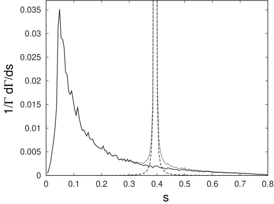
Figure 3: The invariant mass distribution of the two photons in the presence of the $\eta_{c}$ resonance, normalized to the total rate $\Gamma_{\mathrm{tot}}\!=\!5.7\times 10^{-7}$, as obtained for $m_{s}\!=\!0.5$ GeV. We show the pure non-resonant (solid), the pure resonant (dot-dashed) and the total distribution (dashed). The resonance peak is truncated in order to show the relevance of the different contributions both inside and outside the resonance region.

Over these regions we can assume the validity of our perturbative calculation of Section 3 as well as of our previous studies of the various kinematical distributions for $b\rightarrow s\gamma\gamma$ decay [9]. Disregarding in the perturbative calculation of Section 3 the contribution of the resonance region, which we conservatively define as $0.3\leq s\leq 0.5$, we find that the perturbative branching ratio is reduced by at most $14\%$. It would be very useful to verify experimentally that the effect of the $\eta_{c}$ resonance in the $B\rightarrow X_{s}\gamma\gamma$ case is not so relevant, in comparison with what we know to be the case for $B\rightarrow X_{s}e^{+}e^{-}$. In fact, if we consider the decay chain $b\rightarrow s\psi$ followed by $\psi\rightarrow e^{+}e^{-}$ and use both experimental [17] and theoretical [11, 20] inputs, we can estimate that

$$\frac{\Gamma(b\rightarrow s\psi)\Gamma(\psi\rightarrow e^{+}e^{-})}{\Gamma(b\rightarrow se^{+}e^{-})}\simeq 1.4\times 10^{2}\,\,\,,$$ (35)

while the analogous quantity for $b\rightarrow s\eta_{c}$ followed by $\eta_{c}\rightarrow\gamma\gamma$ amounts to

$$\frac{\Gamma(b\rightarrow s\eta_{c})\Gamma(\eta_{c}\rightarrow\gamma\gamma)}{\Gamma(b\rightarrow s\gamma\gamma)}\simeq 6\,\,\,.$$ (36)

This argument indirectly confirms the less dramatic impact that the $\eta_{c}$ resonance has on the invariant mass distribution of the two photons in the $b\rightarrow s\gamma\gamma$ decay.

Appendix A Study of the IR divergences of the rate.

In this appendix we want to show the explicit cancellation between the IR singularities arising respectively in the $b\rightarrow s\gamma\gamma$ rate from the bremstrahlung of a soft photon and in the $O(\alpha_{e})$ virtual corrections to the $b\rightarrow s\gamma$ amplitude. This will confirm our understanding of the endpoints of the photon spectrum in the $b\rightarrow s\gamma\gamma$ decay. Our calculation is very similar to what can be found in Refs. [15, 14] for the study of the gluon spectrum in $b\rightarrow s\gamma g$. Many results could be taken from there provided the different charge and color factors are adequately taken into account. We have indeed reproduced the calculation we report in this appendix and we can confirm a posteriori the results for $b\rightarrow s\gamma g$.

Moreover, as we already explained in Sec. 3, we are not going to include $O(\alpha_{e})$ virtual corrections to the $b\rightarrow s\gamma$ amplitude in the calculation of the rate for $b\rightarrow s\gamma\gamma$. In fact, we will just require the two photons to be hard, imposing a minimun energy cut. Therefore, in the present appendix we will consider only those aspects of the discussion which are necessary to show the cancellation of the IR poles.

In the reaction $b(p)\rightarrow s(p^{\prime})+\gamma(k_{1})+\gamma(k_{2})$, the spectrum of any of the two photons presents two sharp singularities in the vicinity of the endpoints, i.e. for $x_{\gamma}\rightarrow 0$ and for $x_{\gamma}\rightarrow 1$, where we define $x_{\gamma}\!=\!E_{\gamma}/E_{\gamma}^{\rm max}$ for $E_{\gamma}^{\rm max}=(m_{b}^{2}-m_{s}^{2})/2/m_{b}$. The variable $x_{\gamma}$ corresponds in general to the reduced energy of a given photon. To make contact with the notation introduced in (13), we can easily see that :

$$x_{\gamma_{1}}=\frac{u}{1-\rho}=\bar{u}\,\,\,\,\mbox{and}\,\,\,\,x_{\gamma_{2}}=\frac{t}{1-\rho}=\bar{t}\,\,\,\,.$$ (37)

This singular behavior at the endpoints of the spectrum corresponds to the presence of IR singularities in the rate for $b\rightarrow s\gamma\gamma$, when the energy of one or the other of two photons goes to zero, i.e. when $x_{\gamma}\rightarrow 0$ (the energy of the photon under consideration) or $x_{\gamma}\rightarrow 1$ (the energy of the other photon).

These IR singularities originate from the integration of the $A_{77}$ part of the square amplitude over the phase space of the two photons. As we can see from Eq. (3), $A_{77}$ is symmetric with respect to $(\bar{u}\leftrightarrow\bar{t})$, i.e. under the exchange of the two photons. Therefore the treatment of the two endpoints is symmetric. Given the spectrum of one photon, we will arbitrarily consider the endpoint $x_{\gamma_{1}}\rightarrow 1$. All our results will be valid in an analogous manner for the other endpoint, i.e. for $x_{\gamma_{2}}\rightarrow 1$.

Let us consider the contribution of $O_{7}$ only to the differential decay rate. Starting from Eq. (16) and working out the integration over the phase space in $D=4-2\epsilon$ dimension we get

$$\frac{d\Gamma_{7}}{d\bar{t}\,d\bar{u}}=(1-\rho)^{2}\frac{1}{4}\frac{\alpha_{e}}{\pi}\Gamma_{0}F_{7}^{2}\frac{(1-\rho)^{-4\epsilon}(8\pi\mu^{2}/m_{b}^{2})^{2\epsilon}}{\Gamma(2-2\epsilon)[\bar{t}\bar{u}(1-f(\bar{t},\bar{u})^{2})^{1/2}]^{2\epsilon}}A_{77}(\bar{t},\bar{u})\,\,\,,$$ (38)

where $A_{77}(\bar{t},\bar{u})$ is given in Eqs. (3) and (3) and the function

$$f(\bar{t},\bar{u})=1-\frac{2(\bar{u}+\bar{t}-1)}{(1-\rho)\bar{t}\bar{u}}$$ (39)

corresponds kinematically to the cosinus of the angle between the two photons in the rest frame of the b quark, when expressed in terms of the invariants $\bar{u}$ and $\bar{t}$. Moreover we denote by $\Gamma_{0}$ the quantity

$$\Gamma_{0}=\frac{G_{F}^{2}\alpha_{e}|\lambda_{t}|^{2}}{32\pi^{4}}m_{b}^{5}\,\,\,.$$ (40)

The origin of the singularity in $\bar{u}\rightarrow 1$ becomes evident after we integrate over $\bar{t}$ and similarly for the singularity in $\bar{t}\rightarrow 1$ when we integrate over $\bar{u}$. In particular, they are generated by the the first bracket in $A_{77}^{(2)}$ (see Eq. (3)), whose contribution, upon integration, reads

$$\frac{d\Gamma_{7,\bar{u}}^{\rm IR}}{d\bar{u}}=(1+\rho)(1-\rho)^{3}\frac{1}{4}\frac{\alpha_{e}}{\pi}\Gamma_{0}F_{7}^{2}C_{\epsilon}\left[-\frac{2(G^{(a)}+\epsilon G^{(b)})}{(1-\bar{u})^{1+2\epsilon}}\right]\,\,\,,$$ (41)

where

$$C_{\epsilon}=\frac{(1-\rho)^{-4\epsilon}(4\pi\mu^{2}/m_{b}^{2})^{2\epsilon}}{\Gamma(2-2\epsilon)\bar{u}^{2\epsilon}}\,\,\,,$$ (42)

and

$$G^{(a)} = \left(1+\frac{\rho}{1-u}\right)\bar{u}+\frac{1+\rho}{1-\rho}\log(1-u)\,\,\,,$$ (43)

$$G^{(b)} = \frac{\rho}{1-u}\left[2+\log(1-u)\right]\bar{u}-2\frac{1-u}{1-\rho}\log(1-u)+\frac{1+\rho}{1-\rho}\left[\frac{1}{2}\log^{2}(1-u)-2\mbox{Li}_{2}(u)\right]\,\,\,,$$

using the standard notation for the Spence function $\mbox{Li}_{2}(x)=-\int_{0}^{1}dt\log(1-xt)/t$. After the last integration over $\bar{u}$, the IR singularity for $\bar{u}\rightarrow 1$ appears as a pole in $\epsilon$, i.e.

$$\Gamma_{7,\bar{u}\rightarrow 1}^{\mathrm{IR}}(b\rightarrow s\gamma\gamma)=\int_{0}^{1}d\bar{u}\frac{d\Gamma_{7,\bar{u}}^{\mathrm{IR}}}{d\bar{u}}=(1+\rho)(1-\rho)^{3}\frac{1}{4}\frac{\alpha_{e}}{\pi}\Gamma_{0}F_{7}^{2}\frac{1}{\epsilon}\left[2+\frac{1+\rho}{1-\rho}\log\rho\right]\,\,+\,\,\cdots\,\,\,,$$ (44)

where the dots indicate all other kinds of terms arising from the integration. An analogous singularity arises for $\bar{t}\rightarrow 1$ when we integrate the second term of $A_{77}^{2}$ (see Eq. (3)) first over $d\bar{u}$ and then over $d\bar{t}$. Therefore the rate has a total IR singularity given by

$$\Gamma_{7}^{\mathrm{IR}}(b\rightarrow s\gamma\gamma)=\int_{0}^{1}d\bar{u}\frac{d\Gamma_{7}^{\mathrm{IR}}}{d\bar{u}}=(1+\rho)(1-\rho)^{3}\frac{1}{2}\frac{\alpha_{e}}{\pi}\Gamma_{0}F_{7}^{2}\frac{1}{\epsilon}\left[2+\frac{1+\rho}{1-\rho}\log\rho\right]\,\,+\,\,O(1)\,\,\,,$$ (45)

where we have indicated with $O(1)$ all the other non singular terms arising from the integration.

We will now show that the same IR singularity, but with opposite sign, arises from the $O(\alpha_{e})$ virtual corrections to the $b\rightarrow s\gamma$ amplitude induced, of course, by the same operators $O_{7}$. In this case, given the tree level $bs\gamma$ vertex induced by $O_{7}$, we have to consider both self-energy and vertex $O(\alpha_{e})$ corrections in the renormalized theory, i.e. taking into account the wave function renormalization constants of the b and of the s quark. The choice of gauge for the photon is not relevant if the calculation is consistently performed (we checked the result in both the Feynman and the Landau gauge) and the final result reads

$$\Gamma_{7}^{(\alpha_{e})}(b\rightarrow s\gamma) = (1+\rho)(1-\rho)^{3}\Gamma_{0}F_{7}^{2}(1+2K_{\alpha_{e}})\frac{\Gamma(1-\epsilon)}{\Gamma(2-2\epsilon)}\left(\frac{4\pi}{m_{b}^{2}}\right)^{\epsilon}(1-\rho)^{-2\epsilon}$$ (46)

$$= \,\,\,\,\ \Gamma_{7}^{(0)}+\delta\Gamma_{7}^{(\alpha_{e})}\,\,\,,$$

where

$$\Gamma_{7}^{(0)}(b\rightarrow s\gamma) = (1+\rho)(1-\rho)^{3}\Gamma_{0}F_{7}^{2}\,\,\,,$$ (47)

$$\delta\Gamma_{7}^{(\alpha_{e})}(b\rightarrow s\gamma) = (1+\rho)(1-\rho)^{3}\Gamma_{0}F_{7}^{2}2K_{\alpha_{e}}\frac{\Gamma(1-\epsilon)}{\Gamma(2-2\epsilon)}\left(\frac{4\pi}{m_{b}^{2}}\right)^{\epsilon}(1-\rho)^{-2\epsilon}\,\,\,,$$

and

$$K_{\alpha_{e}}=\frac{1}{4}\frac{\alpha_{e}}{\pi}(4\pi)^{\epsilon}\Gamma(1+\epsilon)\left[-\frac{1}{\epsilon}\left(2+\frac{1+\rho}{1-\rho}\log\rho\right)\,\,+\,\,O(1)\right]\,\,\,.$$ (48)

It is now easy to verify that the pole terms cancel between Eq. (45) and Eq. (46), such that

$$\Gamma_{7}^{\rm IR}(b\rightarrow s\gamma\gamma)+\delta\Gamma_{7}^{(\alpha_{e})}(b\rightarrow s\gamma)=O(1)\,\,\,.$$ (49)

In the previous discussion we may have disregarded terms of $O(\epsilon)$ when they do not happen to multiply a quantity containing $1/\epsilon$ poles and we have omitted all over a factor of $(m_{b}(m_{b})/m_{b})^{2}$ because it would not influence the cancellation of the IR poles.

References

[1] B. Grinstein, R. Springer, and M. Wise,
Nucl. Phys. B339 (1990) 269; R. Grigjanis, P.J. O’Donnel,
M. Sutherland and H. Navelet, Phys. Lett. B213 (1988) 355;
Phys. Lett. B286 (1992) E, 413; G. Cella, G. Curci, G. Ricciardi and
A. Viceré, Phys. Lett. B325 (1994) 227, Nucl. Phys. B431 (1994) 417;
M. Misiak, Nuc. Phys B393 (1993) 23, Erratum B439 (1995)
461;
M. Ciuchini, E. Franco, G. Martinelli, L. Reina and L.
Silvestrini, Phys. Lett. B316 (1993) 127; Nucl. Phys. B421 (1994) 41.
[2] K.G. Chetyrkin, M. Misiak and M. Münz,
hep-ph/9612313.
[3] M. Ciuchini, E. Franco, G. Martinelli, L. Reina
and L. Silvestrini, Phys. Lett. B316 (1993) 127; Nucl. Phys. B421 (1994)
41;
A.J. Buras, M. Misiak, M. Münz and S. Pokorski, Nucl. Phys. B424
(1994) 374.
[4] A.F. Falk, M. Luke and M.J. Savage, Phys. Rev. D49
(1994) 3367.
[5] M.B. Voloshin, Phys. Lett.B397 (1997) 275; Z. Ligeti,
L. Randall and M. Wise, hep-ph/9702322; A.K. Grant, A.G. Morgan,
S. Nussinov and R.D. Peccei hep-ph/9702380; G. Buchalla, G. Isidori
and S.J. Rey, hep-ph/9705253.
[6] G.-L. Lin, J. Liu and Y.-P. Yao, Phys. Rev. D42 (1990) 2314.
[7] H. Simma and D. Wyler, Nucl. Phys. B344 (1990) 283.
[8] S. Herrlich and J. Kalinowski, Nucl. Phys. B381 (1992) 501.
[9] L. Reina, G. Ricciardi and A. Soni, Phys. Lett. B396
(1997) 231.
[10] M. Acciarri et al., (L3 Collaboration), Phys. Lett. B363
(1995) 127.
[11] G. Buchalla, A.J. Buras and M.E. Lautenbacher,
Rev. Mod. Phys. 68 (1996) 1125.
[12] B. Grinstein, R. Springer and M.B. Wise, Nucl. Phys. B339 (1990) 269.
[13] H. Simma, Zeit. Phys. C61 (1994) 67.
[14] N. Pott, Phys. Rev. D54 (1996) 938.
[15] A. Ali and C. Greub, Phys. Lett. B259 (1991) 182;
Zeit. Phys. C49 (1991) 431; Phys. Lett. B361 (1995) 146.
[16] T. Inami and C.S. Lim, Prog. Th. Phys. 65
(1981) 297; Erratum, ibidem, 1772.
[17]Review of Particle Physics, Phys. Rev. D54 (1996).
[18] N.G. Deshpande and J. Trampetic, Phys. Lett. B339
(1994) 270