Techniques for computing two-loop QCD corrections to $b\to c$ transitions

Abstract

We have recently presented the complete ${\cal O}(\alpha_{s}^{2})$ corrections to the semileptonic decay width of the $b$ quark at maximal recoil. Here we discuss various technical aspects of that calculation and further applications of similar methods. In particular, we describe an expansion which facilitates the phase space integrations and the treatment of the mixed real–virtual corrections, for which Taylor expansion does not work and the so-called eikonal expansion must be employed. Several terms of the expansion are given for the ${\cal O}(\alpha_{s}^{2})$ QCD corrections to the differential semileptonic decay width of the $b$–quark at maximal recoil. We also demonstrate how the light quark loop corrections to the top quark decay rate can be obtained using the same methods. We briefly discuss the application of these techniques to the calculation of the ${\cal O}(\alpha_{s}^{2})$ correction to zero recoil sum rules for heavy flavor transitions.

I Introduction

Precise determination of $|V_{cb}|$, a parameter of the Cabibbo-Kobayashi-Maskawa (CKM) matrix, is an important goal of many experimental studies. The current experimental limit [1]

$$|V_{cb}|=0.036\mbox{ to }0.046\quad(90\%\mbox{ CL})$$ (1)

is based on measurements of the beauty hadron decays produced at the $\Upsilon(4S)$ resonance (by ARGUS and by CLEO II) and in $Z$-boson decays (by the four experiments at LEP). In the future large samples of the $b$-hadrons collected at $B$-factories (at SLAC and KEK) and at the hadron colliders will increase the statistical accuracy to a few percent level. To fully exploit the anticipated experimental improvement, the theoretical description of the $b$ decay must be known with comparable precision.

There are two methods of extracting the value of $|V_{cb}|$, based on measurements of the exclusive decay $B\to\bar{D^{\star}}\bar{l}\nu_{l}$ and of the inclusive semileptonic decay width of $b$-hadrons $\Gamma_{\rm sl}$. These two methods rely on very different theoretical considerations and experimental procedures and complement each other. Their merits and theoretical uncertainties are summarized e.g. in Ref. [2, 3]. One of the major sources of the theoretical error are the perturbative QCD corrections at the two loop level. For the exclusive decays at the zero recoil point these corrections have recently been calculated [4, 5]. This has significantly improved the accuracy of the theoretical prediction for the exclusive method.

Regarding the inclusive method, recently the ${\cal O}(\alpha_{s}^{2})$ corrections to differential semileptonic decay width of the $b$–quark at maximal recoil have been calculated [6]. Combined with the previously obtained value at zero (minimal) recoil, these results permitted an estimate of the complete ${\cal O}(\alpha_{s}^{2})$ correction to the total semileptonic decay width of the $b$–quark.

In the paper [6] we presented the results of that calculation and discussed its phenomenological relevance. The purpose of the present paper is a detailed description of the methods employed in that calculation. We would like to note that a complete calculation of two-loop corrections to a fermion decay width has never been performed before, neither in QCD nor in QED (a longstanding example are the two-loop QED corrections to the muon life time). Therefore, in the calculation we describe here we had to go beyond the traditional methods used in higher–orders calculation. We hope that a description of some technical aspects and methods will be of interest for the community.

Let us first mention the difficulties one encounters when trying to compute the fourth order corrections to the fermion decays. One of the problems is an appropriate treatment of the real radiation of one or two gluons. For the virtual radiative corrections there exists a number of algorithms, permitting an efficient, analytical treatment of a large number of complicated diagrams, which typically appear in such calculations. On the contrary, no similar algorithms were available so far for the treatment of the real radiation.

The reason why the real radiation at order ${\cal O}(\alpha^{2}_{s})$ is difficult to evaluate is that the particle in the initial state (the decaying $b$ quark) carries a color charge and therefore can radiate. It is the presence of the massive propagator of the initial quark which makes the integrations over the phase space very tough. The kinematical configuration, where the invariant mass of the leptons is equal to zero and the quark in the final state is massive is the first case where a complete analytical evaluation of the real radiation of two gluons in a decay of a fermion turns out possible.

Another potential problem is the treatment of diagrams which represent one–loop virtual corrections to a single gluon emission in the $b$–quark decay. The virtual corrections in such situation are one–loop. Therefore one might naively expect that this case does not require any sophisticated investigation. Unfortunately, the integration of the one–loop formulas (especially of the boxes) over the three body phase space is difficult. However, it turns out possible to express the result for the loop as an expansion which can be easily integrated over the phase space. With a systematic algorithm for the expansion, this approach shifts the burden of the calculation to the computer.

The idea which permitted us to calculate the contribution of the real radiation of one or two gluons is (qualitatively speaking) the expansion in the velocity of the final quark. In the limit $m_{c}\to m_{b}$ the charm quark in the final state is a slowly moving particle, with spatial components of its momentum of the order of $m_{b}-m_{c}$, much smaller than its mass. The momenta of gluons and of leptons (in the case when the invariant mass of the leptons is zero) are also of the order of $m_{b}-m_{c}$. It turns out that by a proper choice of the phase space variables one can systematically expand the amplitudes and the phase space in $\delta\equiv(m_{b}-m_{c})/m_{b}\ll 1$ (sometimes we also use an equivalent expansion parameter $\beta\equiv(m_{b}^{2}-m_{c}^{2})/m_{b}^{2}=\delta(2-\delta)$; throughout this paper we use $m_{b}$ as the unit of mass, putting $m_{b}=1$). The details of the phase space parameterization will be explained in detail.

A word of caution is in order here. Our technique proved to be very useful in problems where the mass of the quark in the final state does not differ too much from the mass of the quark in the initial state. In this respect an ideal application are semileptonic $b\to c$ transitions. On the other hand, for such problems as muon or top quark decay, the expansion parameter may be close to unity and it is not clear at present if our procedure is of any use there. We will, however, show an example where our procedure remains meaningful and delivers reliable predictions even in the case when the expansion parameter equals unity.

The paper is organized as follows. In the next section we discuss how the real radiation of two gluons can be computed. Section III is devoted to the treatment of tensor integrals. Then we present a detailed study of one–loop virtual corrections to a single gluon emission in the $b$–decay. We show that in such diagrams a new type of Feynman integrals appears and discuss their evaluation. Section V is devoted to the applications of our techniques. We present the result for the ${\cal O}(\alpha_{s}^{2})$ correction to the differential semileptonic decay width $b\to c\;l\;\nu_{l}$ up to $\delta^{11}$. We also demonstrate how the known light quark corrections to the top quark decay width can be obtained with good accuracy if the expansion up to high powers of $\delta$ is performed, and discuss an application of our technique to corrections to the zero recoil sum rules. In the last section we present conclusions.

II Emission of two gluons in semileptonic ${b}$ decays

We first consider the radiation of two real gluons in a semileptonic $b$–decay

$$b\to c+e+\nu_{e}+g_{1}+g_{2}$$

and discuss how its contribution to the width can be computed.

Throughout this paper we denote the particles and their four-momenta by the same letters, i.e. the momentum of the $b$–quark is $b$ etc. Moreover, we denote the momentum of the lepton pair $e+\nu_{e}$ as $W$ and often speak about the decay $b\to c+W$. All formulas in this paper apply to the case when the invariant mass of the leptons is zero, i.e. $W^{2}=0$, if not stated otherwise.

Our aim is to construct an expansion in $\delta=(m_{b}-m_{c})/m_{b}\ll 1$. In this case the spatial momentum of the $c$ quark is of the order of $m_{b}-m_{c}$. The momenta of the lepton pair and of the gluons are also of the order of $m_{b}-m_{c}$ because $W^{2}=g_{1}^{2}=g_{2}^{2}=0$. The smallness of these momenta permits an expansion in terms of $\delta$.

A Expansion of the propagators

To show that such an expansion is indeed possible, we list here all propagators of the virtual particles which appear in a calculation of the two gluon emission in the semileptonic $b$–decay:

$$P_{1} = \frac{1}{(b-g_{1})^{2}-m_{b}^{2}}=\frac{1}{-2bg_{1}},\qquad P_{2}=\frac{1}{(b-g_{2})^{2}-m_{b}^{2}}=\frac{1}{-2bg_{2}},$$ (2)

$$P_{3} = \frac{1}{(b-g_{1}-g_{2})^{2}-m_{b}^{2}}=\frac{1}{-2b(g_{1}+g_{2})+2g_{1}g_{2}}$$ (3)

$$P_{4} = \frac{1}{(c+g_{1})^{2}-m_{c}^{2}}=\frac{1}{2cg_{1}},\qquad P_{5}=\frac{1}{(c+g_{2})^{2}-m_{c}^{2}}=\frac{1}{2cg_{2}},$$ (4)

$$P_{6} = \frac{1}{(c+g_{1}+g_{2})^{2}-m_{c}^{2}}=\frac{1}{2c(g_{1}+g_{2})+2g_{1}g_{2}},\qquad P_{7}=\frac{1}{(g_{1}+g_{2})^{2}}=\frac{1}{2g_{1}g_{2}}$$ (5)

All these propagators are shown in the examples in Fig. 1. If we eliminate the momentum of the $c$ quark using momentum conservation, $c=b-W-g_{1}-g_{2}$, we can expand the propagators $P_{4}...P_{6}$ in the Taylor series with respect to the “small” momenta $g_{1}$, $g_{2}$, $W$. Explicitly, we have

$$P_{4} = \frac{1}{2bg_{1}}\sum_{j=0}^{\infty}\frac{(2g_{1}W+2g_{1}g_{2})^{j}}{(2bg_{1})^{j}},\qquad P_{5}=\frac{1}{2bg_{2}}\sum_{j=0}^{\infty}\frac{(2g_{2}W+2g_{1}g_{2})^{j}}{(2bg_{2})^{j}},$$ (6)

$$P_{6} = \frac{1}{2b(g_{1}+g_{2})-2g_{1}g_{2}}\sum_{j=0}^{\infty}\frac{[2(g_{1}+g_{2})W]^{j}}{[2b(g_{1}+g_{2})-2g_{1}g_{2}]^{j}}.$$ (7)

From these expressions we see that the expansion does not generate any new infrared divergences and, therefore, appears to be permissible. After this expansion only four different types of denominators remain. We list them for clarity:

$$P_{1}^{0} \equiv \frac{1}{2bg_{1}},\qquad P_{2}^{0}\equiv\frac{1}{2bg_{2}},$$ (8)

$$P_{3}^{0} \equiv \frac{1}{2b(g_{1}+g_{2})-2g_{1}g_{2}},\qquad P_{7}=\frac{1}{2g_{1}g_{2}}.$$ (9)

As will become clear from the discussion below, it is more convenient to use $P_{3}^{0}$ as one of the basic propagators than to expand it any further.

Let us emphasize at this point the advantages of the above expansion. As can be seen from the above expressions, the four–momentum of lepton pair $W$ and the momentum of the $c$–quark do not appear in the denominator. This immediately implies that the integral over the phase space of $W$ and $c$ factorizes. Therefore, the expansion suggests a simple way how the rather nontrivial integration over the phase space of four particles in the final state can be reduced to a more familiar case of the three body phase space. This reduction is described in the next section.

B Phase–space integration for the emission of two gluons

After we have checked that the propagators of all virtual particles can be expanded, the same must be demonstrated for the phase space element. This is done in the present section.

Considering the semileptonic decay of the $b$–quark and integrating first over the lepton phase space, one obtains the following phase space integration element (we consider only the point where the invariant mass of the lepton pair $W^{2}$ is zero):

$${\rm d}R_{4}=[dc][dW][dg_{1}][dg_{2}]\delta^{D}(b-c-g_{1}-g_{2}-W),$$

where a shorthand notation is

$$[dp]=\frac{{\rm d}^{D-1}p}{2p^{0}},\qquad D=4-2\epsilon.$$

It is convenient to introduce an auxiliary vector $H$ which equals to the sum of the momenta of the $c$–quark and $W$ boson, $H\equiv c+W$. With this notation the phase space integral becomes

$$dR_{4}=\int dH^{2}\int[dH][dg_{1}][dg_{2}]\delta^{D}(b-H-g_{1}-g_{2})\int[dW][dc]\delta^{D}(H-W-c).$$

The integration over the $(W,c)$ phase space gives (for now we assume the integrand contains no $W$ in the numerator; the tensor integrals with $W$ dependence will be analyzed in section III)

$$R_{2}^{Wc}=\int[dW][dc]\delta^{D}(H-W-c)=\frac{\Omega_{D-1}}{2^{D-1}}\frac{(H^{2}-m_{c}^{2})^{D-3}}{(H^{2})^{D/2-1}}$$

where

$$\Omega_{D-1}=\frac{2~{}~{}\pi^{3/2-\epsilon}}{\Gamma(3/2-\epsilon)}$$

is the volume of a $D-1$ dimensional sphere of a unit radius.

Having performed the integration over the $(W,c)$ phase space we are left with the three particle phase space of one massive ($H$) and two massless ($g_{1}$, $g_{2}$) particles and the integration over the square of the momentum $H$.

We use the variables (with $m_{b}^{2}\equiv 1$)

$$H^{2}=y,\qquad(g_{1}+g_{2})^{2}=u,\qquad(H+g_{2})^{2}=z,$$ (10)

and get the following expression for the four particle phase space [7]

$${\rm d}R_{4}=\Bigg{(}\frac{\Omega_{D-1}}{2^{D-1}}\Bigg{)}^{3}\frac{1}{B(1-\epsilon,1-\epsilon)}\int{\rm d}y{\rm d}z{\rm d}uu^{-\epsilon}z^{-\epsilon}(u_{m}-u)^{-\epsilon}\frac{(y-m_{c}^{2})^{1-2\epsilon}}{y^{1-\epsilon}},$$ (11)

with $u_{m}=(1-z)(z-y)/z$ and the following limits of integrations

$$m_{c}^{2}<y<1,\qquad y<z<1,\qquad 0<u<u_{m}.$$ (12)

In order to expand the phase space element in powers of $\beta=(m_{b}^{2}-m_{c}^{2})/m_{b}^{2}$ it is useful to change the variables in the above expression

$$y = 1-\beta x_{1},\qquad z=1-\beta x_{1}x_{2},\qquad u=u_{m}x_{3},$$ (13)

$$u_{m} = \frac{\beta^{2}x_{1}^{2}x_{2}(1-x_{2})}{1-\beta x_{1}x_{2}}.$$ (14)

The integration limits for all $x_{i}$ are the same:

$$0<x_{i}<1$$

Expressing the phase–space element through these variables and restoring proper dimensionality we find:

$${\rm d}R_{4}=R_{4}^{0}~{}\beta^{5-6\epsilon}\int_{0}^{1}{\rm d}x_{1}{\rm d}x_{2}{\rm d}x_{3}J(x_{1},x_{2},x_{3})\Bigg{[}\frac{1}{(1-\beta x_{1}x_{2})^{1-\epsilon}}\frac{1}{(1-\beta x_{1})^{1-\epsilon}}\Bigg{]},$$

where

$$J(x_{1},x_{2},x_{3}) = x_{1}^{3-4\epsilon}(1-x_{1})^{1-2\epsilon}x_{2}^{1-2\epsilon}(1-x_{2})^{1-2\epsilon}x_{3}^{-\epsilon}(1-x_{3})^{-\epsilon},$$ (15)

$$R_{4}^{0} = \frac{(m_{b}^{2})^{2-3\epsilon}}{B(1-\epsilon,1-\epsilon)}\Bigg{(}\frac{\Omega_{D-1}}{2^{D-1}}\Bigg{)}^{3}.$$ (16)

Our final aim is to expand ${\rm d}R_{4}$ in the limit of $m_{c}\to m_{b}$. The above expression is well suited for this purpose. Expanding it in powers of $\beta=(m_{b}^{2}-m_{c}^{2})/m_{b}^{2}$ gives rise to simple integrals which can be expressed by Beta functions:

$$\int{\rm d}x_{1}~{}{\rm d}x_{2}~{}{\rm d}x_{3}J(x_{1},x_{2},x_{3})x_{1}^{n}x_{2}^{m}x_{3}^{k}$$ (18)

$$\qquad\qquad=B(n+4-4\epsilon,2-2\epsilon)B(m+2-2\epsilon,2-2\epsilon)B(k+1-\epsilon,1-\epsilon).$$

C Basic propagators

The basic propagators $P_{1}^{0}$, $P_{2}^{0}$, $P_{3}^{0}$, and $P_{7}$, expressed in terms of the variables $\{x_{i}\}$ yield simple expressions which can be integrated over the phase space. We find

$$P_{1}^{0} = \frac{1}{2bg_{1}}=\frac{1}{\beta x_{1}x_{2}},\qquad P_{2}^{0}=\frac{1}{2bg_{2}}=\frac{1-\beta x_{1}x_{2}}{\beta x_{1}(1-x_{2})[1-\beta x_{1}x_{2}(1-x_{3})]},$$ (19)

$$P_{3}^{0} = \frac{1}{2b(g_{1}+g_{2})-2g_{1}g_{2}}=\frac{1}{\beta x_{1}},\qquad P_{7}=\frac{1}{2g_{1}g_{2}}=\frac{1-\beta x_{1}x_{2}}{\beta^{2}x_{1}^{2}x_{2}(1-x_{2})x_{3}}.$$ (20)

Clearly, the expansion of these quantities in terms of small $\beta$ is readily performed. The resulting integrals are very similar to the integrals in eq. (18) and can be expressed in terms of the Beta functions.

The same is true for all scalar products of the four momenta which enter the calculation. Therefore, the above discussion demonstrates that the part of the semileptonic decay width of the $b$–quark containing radiation of two gluons can be calculated by expanding the matrix element and the four particle phase space in powers of $\beta$. What is still missing in our discussion is the study of the integrals over the $(W,c)$ phase space when the numerator depends on $W$. We discuss this issue in the next section.

III Tensor integrals

The expansion of the propagators in terms of the momenta $W$, $g_{1}$, $g_{2}$, may result in high powers of the scalar products $(Wg_{1})^{a}(Wg_{2})^{b}$, which have to be integrated over the $(W,c)$ phase space. In this section we present efficient methods for such integrations. The results of this section are not restricted to the case $W^{2}=0$ and are likely to be useful for solving other problems.

The main object we are going to discuss is the following integral over the $(W,c)$ phase space:

$$I(a,b) = \int[dW][dc]\delta^{D}(H-W-c)(Wg_{1})^{a}(Wg_{2})^{b}$$ (21)

$$\equiv \langle(Wg_{1})^{a}(Wg_{2})^{b}\rangle_{H=W+c}$$ (22)

for arbitrary $a,b>0$. This integral can be rewritten as

$$I(a,b) = g_{1}^{\mu_{1}}....g_{1}^{\mu_{a}}~{}g_{2}^{\mu_{a+1}}....g_{2}^{\mu_{a+b}}~{}T_{\mu,a+b}$$ (23)

$$T_{\mu,n} \equiv \langle W_{\mu_{1}}....W_{\mu_{n}}\rangle_{H=W+c}.$$ (24)

The important property of the tensor $T$ is that it depends on a single external vector only ($H$). This property simplifies the calculation of the necessary integrals. We discuss below two approaches to such calculation; their relative merits depend on the capabilities of the symbolic manipulation languages, if the algorithm is to be implemented using a computer.

A Method 1

The first approach is more general and potentially more efficient. To fully exploit the dependence on the single external momentum we can extract the component of the vector $W$ which is parallel to it. For this purpose we write:

$$W=W_{\bot}+c_{1}H,\qquad W_{\bot}H=0,\qquad~{}c_{1}=\frac{WH}{H^{2}}$$ (25)

The value of $c_{1}$ is then fixed, because in the general case $W^{2}\neq 0$ we have

$$WH=\frac{1}{2}(H^{2}+W^{2}-m_{c}^{2}).$$ (26)

Therefore, if we use the above substitution for $W$ in the tensor integral $T^{\mu,n}$, we obtain a sum of tensor integrals over transverse components of the $W$ (with respect to $H$):

$$T_{\bot}^{\mu,n}\equiv\langle W_{\bot}^{\mu_{1}}.....W_{\bot}^{\mu_{n}}\rangle_{H=W+c}.$$ (27)

Evidently, the tensor structure of this integral is trivial: since $W_{\bot}H=0$, $T_{\bot}^{\mu,n}$ must be proportional to the absolutely symmetric tensor of the $(D-1)$ dimensional space. The “building block” is the metric tensor of $(D-1)$ dimensional space: $g_{\mu\nu}-H_{\mu}H_{\nu}/H^{2}$. We note that only tensors of even rank contribute. The generation of the absolutely symmetric tensor of $D-1$ dimensional space can be easily encoded in a symbolic manipulation program. Hence, the algorithm described above permits an efficient treatment of the tensor integrals which appear in the problem at hand.

B Method 2

Using the same idea as in the previous section we can advance slightly further with the analytical calculation of the integral $I(a,b)$.

After writing $W=W_{\bot}+c_{1}H$ and noticing that $g_{1}H$ and $g_{2}H$ are constants in the $(W,c)$ phase space, we conclude that the non-trivial integrals to be computed are

$$I_{\bot}(a,b)\equiv\langle(W_{\bot}g_{1})^{a}(W_{\bot}g_{2})^{b}\rangle_{H=W+c}=\langle(W_{\bot}g_{1\bot})^{a}(W_{\bot}g_{2\bot})^{b}\rangle_{H=W+c},$$ (28)

with $g_{i\bot}$ (i=1,2) defined in analogy to $W_{\bot}$.

The integral $I_{\bot}$ is a Lorentz–scalar and we can choose an arbitrary frame for its calculation. For instance, we consider $H$ to have only the zeroth component and put the $z$–axis of the $D-1$ dimensional space along the vector $g_{1\bot}$. Then, rewriting $g_{2\bot}$ as

$$g_{2\bot}=g_{2a}+c_{2}g_{1\bot},\qquad g_{2a}g_{1\bot}=0,\qquad c_{2}=g_{2\bot}g_{1\bot}/g_{1\bot}^{2},$$ (29)

we find that $I_{\bot}$ is expressed as a sum of integrals of the from:

$$I_{1}(a,b)=\langle(W_{\bot}g_{1\bot})^{a}(W_{\bot}g_{2a})^{b}\rangle_{H=W+c}.$$ (30)

This integral is non-zero only if both $a$ and $b$ are even integers.

Since $g_{2a}g_{1\bot}=0$, we can put the $x$-axis of the $D-1$ dimensional space along the vector $g_{2a}$. Then we have:

$$I_{1}(a,b) = R_{2}^{Wc}|W_{\bot}|^{(a+b)}|g_{1\bot}|^{a}|g_{2a}|^{b}I_{2}(a,b)$$ (31)

$$I_{2}(a,b) = \int\frac{d\Omega_{D-1}}{\Omega_{D-1}}\Bigg{(}\frac{W_{\bot}g_{1\bot}}{|W_{\bot}||g_{1\bot}|}\Bigg{)}^{a}\Bigg{(}\frac{W_{\bot}g_{2a}}{|W_{\bot}||g_{2a}|}\Bigg{)}^{b}.$$ (32)

The integration element is

$${\rm d}\Omega_{D-1}=\prod_{i=1}^{D-2}\sin^{D-2-i}\theta_{i}~{}{\rm d}\theta_{i},\qquad 0<\theta_{i}<\pi\quad(i\neq D-2),\qquad 0<\theta_{D-2}<2\pi.$$ (33)

If we choose $z$ and $x$ axes as described above, we get

$$\frac{W_{\bot}g_{1\bot}}{|W_{\bot}||g_{1\bot}|} = -\cos\theta_{1},$$ (34)

$$\frac{W_{\bot}g_{2a}}{|W_{\bot}||g_{2a}|} = -\sin\theta_{1}\cos\theta_{2}.$$ (35)

The minus sign in the above equations arises because the transverse vectors here are spacelike. In calculating $I_{2}(a,b)$ the following formula is useful:

$$\int_{0}^{\pi}{\rm d}\theta\sin^{\alpha}\theta\cos^{\beta}\theta=B\left(\frac{1+\alpha}{2},\frac{1+\beta}{2}\right).$$ (36)

This formula is valid for even and positive $\beta$. Using it we get the result for the integral $I_{2}(a,b)$:

$$I_{2}(a,b)={(-1)^{a+b}\Gamma\left({3\over 2}-\epsilon\right)\Gamma\left({1+a\over 2}\right)\Gamma\left({1+b\over 2}\right)\over\pi\Gamma\left({a+b+3-2\epsilon\over 2}\right)}$$ (37)

In order to use these results for the further integration over the phase space $(H,g_{1},g_{2})$ it is necessary to express the modulus of the vectors $W_{\bot}$, $g_{1\bot}$, $g_{2a}$ in terms of the variables $\{x_{i}\}$ introduced in the previous section. This is a cumbersome but straightforward task and we do not discuss it here in any detail.

The steps described above allow an easy implementation in any symbolic manipulation program. They provide an efficient and uniform treatment of the tensor integrals which appear in this calculation.

IV One loop virtual correction and one real gluon

Another source of the $O(\alpha_{s}^{2})$ corrections are the one–loop virtual corrections accompanied by a radiation of an additional real gluon. Again, we would like to expand those diagrams in powers of $\delta=(m_{b}-m_{c})/m_{b}$. The purpose of this section is to provide a suitable algorithm.

There is a principal difference from the radiation of two real gluons in this part of the corrections. Namely, it is not sufficient here to perform a Taylor expansion of the relevant diagrams.

To see this, let us analyze a simple example. We consider a diagram where the $b$–quark radiates a gluon and then a one–loop self–energy correction is inserted on the $b$ quark line (see Fig. 2). Taking the limit $m_{b}\to m_{c}$ in such situation implies that the momentum of the real gluon goes to zero. Therefore the self–energy diagram should be calculated close to the mass shell of the $b$–quark. It is well–known that in this limit the self–energy diagram has an on-shell logarithmic singularity of the form

$$\log(M^{2}-p^{2})\sim\log(M^{2}-m^{2})\sim\log(\delta).$$

Since this diagram contains $\log(\delta)$ it is clear that it cannot be calculated as a Taylor expansion with respect to $\delta$. Therefore, a more sophisticated procedure is needed and the method of eikonal expansions [8, 9] is used in this case. We illustrate this approach in the following example.

A An example of the eikonal expansion

In this subsection we consider a simple example of a one–loop integral, where a result obtained from the eikonal expansion can be compared with an exact formula. We calculate the scalar self–energy diagram:

$$B(p^{2},m^{2})=\int\frac{{\rm d}^{D}k}{(2\pi)^{D}}\frac{1}{k^{2}[(k+p)^{2}-m^{2}]}.$$ (38)

Performing Feynman parameterization, integrating over the loop momenta, and expanding in $\rho=(m^{2}-p^{2})/p^{2}$ we get (using $p^{2}=1$ here):

$$B(p^{2},m^{2})=\frac{i\Gamma(1+\epsilon)}{(4\pi)^{D/2}}\left(\frac{1}{\epsilon}+2-\rho+\rho\ln\rho-\frac{\rho^{2}}{2}+\frac{\rho^{3}}{6}-\frac{\rho^{4}}{12}+\ldots\right)$$ (39)

The appearance of the $\log(\rho)$ term in this result signals that the Taylor expansion of the integrand will be insufficient. In order to get the correct result we add the eikonal expansion. For this purpose we write

$$B(p^{2},m^{2})=B_{\rm t}+B_{\rm eik}$$ (40)

The Taylor expansion term $B_{\rm t}$ is obtained by expanding the integrand in (38) in a Taylor series in $\rho$. This yields a set of one–loop on–shell integrals which are well known. The validity of such an expansion is determined by the condition $k^{2}+2pk\gg\rho p^{2}$. If this is not the case, the Taylor expansion breaks down. This breakdown gives rise to an infrared singularity which occurs in the region where $\rho p^{2}\sim 2pk$ and $k^{2}\ll\rho p^{2}$. This spurious divergence can be cancelled by adding an expansion of the integrand in $k^{2}$ (for a more detailed discussion see [8, 9]).

One should note in addition that if any power of $k^{2}$ appears in the numerator we get an integral of the form:

$$I(n)=\int\frac{{\rm d}^{D}k}{(2\pi)^{D}}\frac{(k^{2})^{n}}{2pk-p^{2}\rho},\qquad~{}~{}~{}n\geq 0.$$

An important point is that such integrals are zero within the dimensional regularization framework. One simple reason for this is that the integral over transverse components of $k$ is scaleless.

Hence, the only term in the eikonal expansion we should consider is the one with $k^{2}$ neglected in the second propagator. The eikonal integral therefore reads:

$$B_{\rm eik}=\int\frac{{\rm d}^{D}k}{(2\pi)^{D}}\frac{1}{k^{2}(2pk-p^{2}\rho)}.$$ (41)

It is evident that this integral scales with $\rho$ as $B_{\rm eik}\propto\rho^{1-2\epsilon}$. It is this dependence on $\epsilon$ which gives $\log(\rho)$ in the final result.

Consider $B_{\rm eik}$ in the rest frame of $p$. Performing the integration over the time component of the loop momenta first, one gets a simple integral representation over the transverse components of the loop momenta which can be easily calculated. More sophisticated eikonal integrals are considered in the next section, where all necessary formulas can be found.

B Eikonal integrals: preliminaries

Here we provide a set of formulas for dealing with integrals appearing in the eikonal expansions. As is clear from the example presented above, the region of integration in which we are interested here is characterized by the values of the virtual momentum of the order of the momentum of the real gluon emitted in the decay.

We denote the loop momentum by $k$ and the momentum of the real gluon by $g$; explicitly, the eikonal expansion of the propagator

$$P(k)=\frac{1}{(k+b-g)^{2}-m_{b}^{2}}=\frac{1}{k^{2}+2k(b-g)-2bg}$$

is given by

$$P(k)_{\rm eik}=\frac{1}{2kb-2bg}\sum_{0}^{\infty}\left(\frac{2kg-k^{2}}{2kb-2bg}\right)^{j}.$$

The basic eikonal integral in the one–loop correction then reads

$$I^{\pm}(n,m,a,b)=\int\frac{{\rm d}^{D}k}{(2\pi)^{D}}\frac{(kW)^{a}(kg)^{b}}{(k^{2}+i\delta)(2kQ\pm 2Qg+i\delta)^{n}(2kQ+i\delta)^{m}}$$ (42)

In the actual calculation $Q$ is always a time–like vector which for different diagrams can be $b,~{}b-g,~{}c+g$.

As we pointed out above, the integrals with any power of $k^{2}$ in the numerator vanish. There are several ways to see this. First, the integrals over transverse (with respect to $Q$) components of the loop momenta are scaleless; also if there is no $k^{2}$ in the denominator, the poles of the integrand are located only on one side of the $k^{0}$ integration axis. Also, if $n<0$, the integral in eq. (42) is zero because it is scaleless.

Let us describe the most economic way to calculate $I^{\pm}$. We choose the Lorentz frame in which $Q=(Q^{0},0,\ldots,0)$. The integration over the time-like component of the vector $k$ can be performed using the residues. If the integration contour is closed in the upper half–plane, only that pole in $1/k^{2}$ contributes for which $k_{0}=-k_{\bot}$.

After $k_{0}$, the integration over the $D-1$ dimensional space should be performed. To discuss the integration over $k_{\bot}$ we first note that after integrating over $k_{0}$ the denominator of the integral $I^{\pm}(n,m,a,b)$ depends on $k_{\bot}^{2}$ only. Therefore, all tensor integrals which appear due to the numerator structure are simply related to the $D-1$ absolutely symmetric tensor of the corresponding rank. Hence, the tensor integrals here are similar to the ones discussed in Section III.

Finally, we are left with the radial integration over the modulus of $k_{\bot}$. The following formulas are useful:

$$I^{-}(n,m,m_{1}) = \int\frac{{\rm d}^{D}k}{(2\pi)^{D}}\frac{(k_{\bot}^{2})^{m_{1}/2}}{(k^{2}+i\delta)(2kQ-2Qg+i\delta)^{n}(2kQ+i\delta)^{m}}$$ (43)

$$= \frac{i\Omega_{D-1}}{(2\pi)^{D-1}}B(2-m+m_{1}-2\epsilon,n+m-m_{1}-2+2\epsilon)$$ (45)

$$\times(Qg)^{2-m+m_{1}-n-2\epsilon}(Q^{2})^{-1-m_{1}/2+\epsilon}(-1)^{n+m+m_{1}+1}2^{-m-n-1}$$

$$I^{+}(n,m,m_{1}) = \int\frac{{\rm d}^{D}k}{(2\pi)^{D}}\frac{(k_{\bot}^{2})^{m_{1}/2}}{(k^{2}+i\delta)(2kQ+2Qg+i\delta)^{n}(2kQ+i\delta)^{m}}$$ (46)

$$= \frac{i\Omega_{D-1}}{(2\pi)^{D-1}}(Qg)^{2-m+m_{1}-n-2\epsilon}(Q^{2})^{-1-m_{1}/2+\epsilon}$$ (49)

$$\times\frac{(-1)^{n+m+m_{1}+1}2^{-m-n-1}}{(n-1)!}~{}\frac{\Gamma(2-m+m_{1}-2\epsilon)}{\Gamma(3-n-m+m_{1}-2\epsilon)}$$

$$\times\Big{[}\psi(2-m+m_{1}-2\epsilon)-\psi(-1+m-m_{1}+2\epsilon)\Big{]},$$

with

$$\psi(z)=\frac{1}{\Gamma(z)}\frac{{\rm d}\Gamma(z)}{{\rm d}z}.$$ (50)

In the above formulas $\Omega_{D-1}$ is the volume of the $D-1$ dimensional sphere of unit radius.

There is one subtle point concerning the expressions presented above. Namely, it is easy to see that the integrals $I^{+}$ have an additional singularity after the integration over $k_{0}$ has been performed. This singularity corresponds to the appearance of the imaginary part in some of Feynman diagrams which contribute to the result. Below we explain how this singularity was treated.

In the singular integrals the integration over the modulus of the transverse momenta is

$$I^{+}\sim\int_{0}^{\infty}{\rm d}k_{\bot}\frac{k_{\bot}^{\alpha}}{(k_{\bot}-1-i\delta)^{n}}.$$

The singularity is located at the point $k_{\bot}=1$. To make this integral meaningful we rewrite it as

$$I^{+}\sim\left.\frac{1}{(n-1)!}\left(\frac{{\rm d}}{{\rm d}x}\right)^{(n-1)}\int_{0}^{\infty}{\rm d}k_{\bot}\frac{k_{\bot}^{\alpha}}{k_{\bot}-x-i\delta}\right|_{x=1}.$$

Rescaling $k_{\bot}\to x~{}k_{\bot}$ we get:

$$I^{+}\sim\left.\frac{1}{(n-1)!}\left(\frac{{\rm d}}{{\rm d}x}\right)^{(n-1)}x^{\alpha}\int_{0}^{\infty}{\rm d}k_{\bot}\frac{k_{\bot}^{\alpha}}{k_{\bot}-1-i\delta}\right|_{x=1}.$$

For the derivative we use

$$\left(\frac{{\rm d}}{{\rm d}x}\right)^{(n-1)}x^{\alpha}=\frac{\Gamma(1+\alpha)}{\Gamma(2+\alpha-n)}x^{\alpha-n+1}.$$

Finally, after performing the remaining integration over $k_{\bot}$ using

$${\rm Re}\int_{0}^{\infty}{\rm d}x\frac{x^{\alpha}}{x-1+i\delta}=\psi(1+\alpha)-\psi(-\alpha),$$

we arrive at the formula for $I^{(+)}$ quoted above.

C Eikonal integrals for the graphs with the gluon self–coupling

The graphs with a triple gluon coupling lead to the most difficult eikonal integrals. The difficulty originates from the fact that in such graphs one has two massless (gluon) propagators. A typical integral reads

$$\int\frac{{\rm d}^{D}k}{(2\pi)^{D}}\frac{1}{k^{2}~{}(k-g)^{2}~{}((k+b-g)^{2}-m_{b}^{2})((c+k)^{2}-m_{c}^{2})}.$$

The Taylor expansion of such integral is easy. However, in the eikonal expansion one cannot expand massless propagators. Therefore, the master integral in this case is

$$I(n,m)=\int\frac{{\rm d}^{D}k}{(2\pi)^{D}}\frac{1}{k^{2}~{}(k-g)^{2}(2kQ-2Qg)^{n}(2kQ)^{m}},$$

where $Q$ is again a “large” time-like vector, as described in the previous section.

Note also, that in this case the terms with $k^{2}$ or $(k-g)^{2}$ in the numerator do contribute to the result.

Let us describe in detail how such integrals can be calculated. For this purpose we first combine the massless denominators:

$$\frac{1}{k^{2}~{}(k-g)^{2}}=\int_{0}^{1}\frac{{\rm d}x}{(k^{2}-2kgx)^{2}}=\int_{0}^{1}\frac{{\rm d}x}{((k-gx)^{2})^{2}}$$

Next, we decompose the product of two eikonal propagators

$$\frac{1}{(2kQ-2Qg)^{n}(2Qk)^{m}}$$

using partial fractions. The integral $I(m,n)$ becomes now a sum of the integrals of the following type:

$$I_{1}(n) = \int_{0}^{1}~{}{\rm d}x~{}\int\frac{{\rm d}^{D}k}{(2\pi)^{D}}\frac{1}{[(k-gx)^{2}]^{2}(2kQ-2gQ)^{n}},$$ (51)

$$I_{2}(n) = \int_{0}^{1}~{}{\rm d}x~{}\int\frac{{\rm d}^{D}k}{(2\pi)^{D}}\frac{1}{[(k-gx)^{2}]^{2}(2kQ)^{n}}.$$ (52)

In both integrals we shift the integration momentum $k\to k+xg$ and get

$$I_{1}(n) = \int_{0}^{1}~{}{\rm d}x~{}\int\frac{{\rm d}^{D}k}{(2\pi)^{D}}\frac{1}{(k^{2})^{2}[2kQ-2gQ(1-x)]^{n}},$$ (53)

$$I_{2}(n) = \int_{0}^{1}~{}{\rm d}x~{}\int\frac{{\rm d}^{D}k}{(2\pi)^{D}}\frac{1}{(k^{2})^{2}(2kQ+2gQx)^{n}}.$$ (54)

Now, in the first integral one makes the change of variables $x\to 1-x$ and then rescales the integration momenta $k\to xk$ in both $I_{1}$ and $I_{2}$. The integration over $x$ factorizes and can be done using

$$\int_{0}^{1}{\rm d}x\;x^{\alpha}=\frac{1}{\alpha+1}.$$

The integrals over $k$ differ from the integral in the previous section by the presence of two powers of $k^{2}$ in the denominator. In this case it is useful to perform a transformation (similar to the technique of integration by parts [10]), which reduces the integrals with the second power of $k^{2}$ in the denominator to the integrals with the first power only.

To write down this transformation we introduce the notation

$$I^{\pm}(\alpha,n,m)=\int\frac{{\rm d}^{D}k}{(2\pi)^{D}}\frac{1}{(k^{2})^{\alpha}(2kQ\pm 2Qg)^{n}(2kQ)^{m}}.$$

Then

$$I^{\pm}(2,n,m)=Q^{2}~{}\Big{[}-2(m+1)I^{\pm}(1,n,m+2)-2~{}n~{}I^{\pm}(1,n+1,m+1)\Big{]}.$$

Using this formula we end up with integrals with the first power of $k^{2}$ in the denominator, for which the formulas of the previous section are applicable.

D Integration over the single gluon phase space

In the treatment of the radiation of one gluon with ${\cal O}(\alpha_{s}^{2})$ accuracy, the last step one has to do is to perform the integration over the phase space of the real gluon. The eikonal expansion, described above in detail, gives the virtual corrections in terms of powers and logarithms of the small parameters. This form of the intermediate result simplifies the final integration over the phase space of the decay products. This would not be the case if we had an exact result for the loop: that would certainly contain dilogarithms of complicated arguments.

The phase space integration with a single gluon is in its general structure similar to the case of two real gluons, discussed in section II B. For completeness, we give a short account of necessary formulas.

In the present case the phase space element is:

$${\rm d}R_{3} = \int[dc][dW][dg]\delta^{D}(b-c-g-W),$$ (55)

$$= \left(\frac{\Omega_{D-1}}{2^{D-1}}\right)^{2}m_{b}^{2-4\epsilon}\beta^{3-4\epsilon}\int_{0}^{1}{\rm d}xJ(x)\frac{1}{(1-\beta x)^{1-\epsilon}}$$ (56)

$$J(x) = x^{1-2\epsilon}(1-x)^{1-2\epsilon}$$ (57)

with

$$H = W+c,\qquad H^{2}=1-\beta x,$$ (58)

$$bH = 1-\frac{\beta x}{2},\qquad bg~{}=~{}Hg~{}=\frac{\beta x}{2}.$$ (59)

The master integral in this case reads:

$$\int_{0}^{1}{\rm d}xJ(x)x^{n}=B(n+2-2\epsilon,2-2\epsilon).$$ (60)

The results of the eikonal integrals require a slight modification of the master integral. As we saw in section IV B, those results contain $(bg)^{-2\epsilon}$ which results in an extra factor $x^{-2\epsilon}$. In this case the master integral is

$$\int_{0}^{1}{\rm d}xJ(x)x^{n-2\epsilon}=B(n+2-4\epsilon,2-2\epsilon).$$ (61)

V Applications

In this section we discuss some applications of the techniques described above.

First, we give a complete result for the ${\cal O}(\alpha_{s}^{2})$ correction to the differential semileptonic decay width of the $b$–quark at the maximal recoil point. We next re-derive the BLM ${\cal O}(\alpha_{s}^{2})$ corrections to the quark top decay width into massless $W$–boson and $b$ quark with the help of the expansions presented above. As will be explained below, the expansion parameter in this case is unity. It not obvious that the techniques described above can be of any use there. Therefore it is interesting to check how the procedure works in such extreme limit. Finally, we comment on the applications to zero recoil sum rules.

A Two–loop QCD correction to semileptonic $b$–decay at maximal recoil

The measurement of the inclusive semileptonic decay width permits a determination of the CKM matrix parameter $|V_{cb}|$ with a small theoretical uncertainty [2, 3]. The magnitude of the perturbative corrections ${\cal O}(\alpha_{s}^{2})$ to this quantity has been subject of discussions in the recent literature. We addressed this problem in ref. [6] where the exact calculation of the ${\cal O}(\alpha_{s}^{2})$ corrections at maximal recoil was used to estimate the total 4th order correction to the $b$ quark semileptonic width. Here we present more complete results of that calculation.

We consider semileptonic decay of the $b$–quark $b\to cl\nu_{l}$. The momentum carried away by leptons is denoted by $q$. We write differential semileptonic decay width of the decay $b\to cl\nu_{l}$ at $q^{2}=0$ as

$$\left[\frac{{\rm d}\Gamma_{\rm sl}}{{\rm d}q^{2}}\right]_{q^{2}=0}\;=\;\Gamma_{0}\left[\Delta_{\rm Born}+\frac{\alpha_{s}}{\pi}C_{F}\Delta_{1}+\left(\frac{\alpha_{s}}{\pi}\right)^{2}C_{F}\Delta_{2}\right]$$ (62)

where $\Gamma_{0}=\frac{G_{F}^{2}m_{b}^{3}}{96\pi^{3}}|V_{cb}|^{2}$. $\Delta_{\rm Born}=(1-m_{c}^{2}/m_{b}^{2})^{3}$ and $\Delta_{1}$ is also known in a closed analytical form [11, 12]. $\Delta_{2}$ is the new result which gives ${\cal O}(\alpha_{s}^{2})$ correction to the differential semileptonic decay width of the $b$-quark at the point of zero invariant mass of leptons.

For the purpose of the presentation we write the 4th order correction as

$$\Delta_{2}=\delta^{3}\left[(C_{F}-C_{A}/2)\Delta_{F}+C_{A}\Delta_{A}+T_{R}N_{L}\Delta_{L}+T_{R}\Delta_{H}\right].$$ (63)

In the above equation $\delta=(1-m_{c}/m_{b})$ is the expansion parameter. $\Delta_{H}$ describes the contribution of the massive $b$ and $c$ quark loops.

For the $SU(3)$ group the color factors are $C_{A}=3$, $C_{F}=4/3$, $T_{R}=1/2$. $N_{L}$ is the number of light quark flavors whose masses were neglected.

In ref. [6] we have presented analytical results for the functions $\Delta_{F,A,L,H}$ up to $\delta^{4}$, though actual calculations have been done up to $\delta^{8}$. Our complete formulas for these functions are presented in Appendix A.

B BLM ${\cal O}(\beta_{0}\alpha_{s}^{2})$ corrections to the decay width of the top quark

As another application of the above techniques we consider the decay of the top quark $t\to Wb$. It is well known that this decay width (at least at the Born and the one–loop level) can be well approximated by neglecting the masses of the $W$–boson and the $b$–quark. In such case, since $W^{2}=0$, the techniques presented in the main part of this paper can be readily applied. In particular, the formula (62) can be rewritten in such form that it gives the correction to the two-body decay width $t\to QW$ (where $Q$ is a heavy quark):

$$\Gamma(t\to QW)=\widetilde{\Gamma}_{0}\left[\Delta_{\rm Born}+\frac{\alpha_{s}}{\pi}C_{F}\Delta_{1}+\left(\frac{\alpha_{s}}{\pi}\right)^{2}C_{F}\Delta_{2}\right].$$ (64)

The $\Delta_{i}$ functions here are the same as in eq. (62), with $m_{b}$ and $m_{c}$ replaced by $m_{t}$ and $m_{Q}$. The problem, however, is that the procedures described above were based on the expansion of the rate in the mass difference of the final and initial quarks. In the case of the top quark decay with a $b$ quark in the final state this means that the expansion parameter $\delta=(m_{t}-m_{b})/m_{t}$ is close to 1 for realistic values of $m_{t}$ and $m_{b}$.

Little is known about convergence properties of the series described in this paper. Fortunately, part of the ${\cal O}(\alpha_{s}^{2})$ correction to the top quark width is known exactly; it is the contribution of the massless quarks, calculated for $m_{W}=m_{b}=0$ in [13, 14] (the relevant diagrams are shown if Fig. 3). We can use that limiting case to check if we can reproduce it with our techniques.

The exact formula for the massless quark correction reads (in the $\overline{\rm MS}$–scheme and for one generation of massless fermions)

$$\Gamma^{{\rm ferm}}(t\to Wb) = \left(\frac{\alpha_{s}}{\pi}\right)^{2}\frac{C_{F}T_{R}}{16}\widetilde{\Gamma}_{0}\left[2\zeta(3)+\frac{23}{9}\zeta(2)-\frac{8}{9}\right],$$ (65)

$$\widetilde{\Gamma}_{0} = \frac{G_{F}~{}m_{t}^{3}}{8\;\sqrt{2}\;\pi}.$$ (66)

It should be mentioned that the diagrams with real or virtual massless fermions represent the simplest case for the described algorithms. The reason is their simple planar topology, which allows the computer programs to work very fast. For this particular type of diagrams we can expand the width up to a very high power in $\delta$.

We write the result of this expansion as

$$\Gamma^{{\rm ferm}}(t\to bW)=\left(\frac{\alpha_{s}}{\pi}\right)^{2}C_{F}~{}T_{R}\widetilde{\Gamma}_{0}~{}F(\delta),$$

where the function $F(\delta)$ is given as a series of powers and logs of $\delta$; we have computed this expansion up to terms of the order $\delta^{21}$. The first few terms of that expansion are given by the function $\Delta_{L}$ in the appendix.

The numerical value of the exact result is

$$F(1)=\frac{1}{16}\left(2\zeta(3)+\frac{23}{9}\zeta(2)-\frac{8}{9}\right)=0.3574\ldots.$$

The values of the approximate result $F(\delta)$ for $\delta=1$ are, for three numbers $N$ of the summed terms,

$$N = 21,\qquad F(1)=0.3266,$$ (67)

$$N = 15,\qquad F(1)=0.3210,$$ (68)

$$N = 11,\qquad F(1)=0.3176.$$ (69)

Comparing these numbers with the exact result we see that already the first 11 terms of the expansion give the accuracy of about $10\;\%$. Unfortunately, the accuracy does not improve significantly with the growing number of terms in the expansion. This slow convergence of the series is caused by the logarithms of the small ($b$ quark) mass. Although these terms are suppressed by powers of that mass (and should give no contribution to the final result if $m_{b}=0$), they spoil the convergence of the expansion. It would be very useful (and we think it is possible) to find a systematic way of eliminating those parts of the integrands which give rise to these logs.

On the other hand, from the perspective of practical applications (like top physics at the Next Linear Collider) it would be sufficient to know the two–loop QCD correction to the top quark decay width even with $10$ percent accuracy. It is tempting to apply our algorithms to this problem and extrapolate the result to the point $\delta=1$; on the other hand, at present we do not know any reliable method for estimating the uncertainty of such result.

C Zero recoil sum rules for $b\to c$ transition with ${\cal O}(\alpha_{s}^{2})$ accuracy

Another useful application of the techniques described above is connected with the so-called zero recoil (ZR) sum rules [2]. In this subsection we would like to discuss this point. A more detailed discussion of ZR sum rules with the ${\cal O}(\alpha_{s}^{2})$ corrections will be given in a future publication [17].

The ZR sum rules are important for the estimates of the zero recoil transition form factors such as $F_{B\to D^{*}}$ for $B\to D^{*}$ transition or $F_{B\to D}$ for $B\to D$ transition. In turn, the formfactor $F_{B\to D^{*}}$ is a crucial ingredient for $|V_{cb}|$ determination from the exclusive semileptonic $B\to D^{*}l\nu_{l}$ decays.

The sum rules for exclusive heavy–to–heavy flavor transitions are based on the operator product expansion (OPE) of the hadronic amplitudes in terms of the inverse quark masses. The zeroth order term in this expansion is the parton model where free quarks are substituted for real hadrons both in initial and final state. Here we disregard the non-perturbative corrections and discuss how the perturbative corrections ${\cal O}(\alpha_{s}^{2})$ to the sum rules can be evaluated.

We consider a transition of a $b$ quark at rest to a $c$ quark and massless partons which occurs under the influence of the external current $J_{\mu}$. The momentum carried away by the external current is $q=(q_{0},0)$, where

$$q_{0}=m_{b}-m_{c}-\epsilon,\qquad\epsilon\leq\mu\ll m_{b},m_{c}.$$

The quantity which is of primary importance for the perturbative corrections to ZR sum rules can be schematically written as:

$$\int\limits_{0}^{\mu}{\rm d}\epsilon\;w_{J}(\epsilon),~{}~{}~{}w_{J}(\epsilon)=\Gamma_{J}(b\to c+X\;|\;q_{0}).$$

In this equation we have shown explicitly the dependence of the transition rate $\Gamma_{J}(b\to c\;|\;q_{0})$ both on the external momenta transfer $q_{0}$ and on the Lorentz structure of the current.

If $\epsilon=0$, the transition is elastic; the final state is a single $c$–quark at rest. The ${\cal O}(\alpha_{s}^{2})$ corrections in this case reduce to the renormalization of the external current $J_{\mu}$. For vector and axial currents they were calculated in [4, 5].

On the other hand, if $\epsilon\neq 0$ the $c$ quark starts moving and can radiate. The second order corrections ${\cal O}(\alpha_{s})$ were calculated in [2, 15, 16]. Aiming at the fourth order, i.e. at ${\cal O}(\alpha_{s}^{2})$ accuracy, one has to consider the final state with the $c$–quark and two real gluons or light quarks and also the ${\cal O}(\alpha_{s})$ correction to the single gluon emission in $b\to c$ transition.

Due to the hierarchy of scales, $\epsilon<\mu\ll m_{b},m_{c}$, the final $c$–quark is moving slowly by definition; this is therefore a nice place where the techniques described in this paper can be applied. In particular, an algorithm for performing eikonal expansions with the subsequent integration over the phase space appears to be very useful here. This topic will be discussed in detail in ref. [17].

VI Conclusion

In this paper we have described techniques used in the calculation of the ${\cal O}(\alpha_{s}^{2})$ corrections to the semileptonic decay width $b\to cl\nu_{l}$ at maximal recoil [6].

The technical tool we used for that calculation is an expansion of the decay rate in powers and logarithms of the mass difference between the initial and final quarks. We presented a detailed discussion of the algorithm, which enables one to construct such expansion. We treated virtual corrections, emission of one gluon, and emission of two gluons separately. Therefore, these algorithms can be used for the analyses of less inclusive quantities than the total decay rate, at least in principle.

In case of two–loop virtual corrections and emission of two real gluons, the expansion in $\delta=(m_{b}-m_{c})/m_{b}$ is a Taylor expansion. In the case of one–loop corrections to the amplitude of single gluon emission in $b$-decay, the Taylor expansion is insufficient. An appropriate method is provided by the eikonal expansions, recently introduced in refs. [8, 9]. When this procedure is used, a new type of Feynman integrals appears. These integrals and methods which were used for their evaluation were described here in some detail.

The whole construction works well if the mass difference between initial and final state quarks is not too large. This is the case for the semileptonic $b\to c$ transitions, where the expansion parameter $(m_{b}-m_{c})/m_{b}\sim 0.7$. In this case we calculated the expansion up to the eleventh power of $\delta$; the estimated accuracy of the final result is better than $1\%$.

There is, however, a number of other applications where the initial quark is significantly heavier than the final one. It is not obvious to what extend the present method can be useful in such situation. There is an indication, however, that our procedures give meaningful results even in that limit. As an example, we analyzed the light quark corrections to the width of the top quark decay into massless $W$ boson and a $b$-quark. We have shown that the first several terms of the expansion in $\delta_{t}=(m_{t}-m_{b})/m_{t}$ approximate the known exact result with a $10\%$ accuracy.

Finally, we have argued that the same techniques can be applied to the corrections to the zero recoil sum rules for the heavy flavor transitions.

A Results for the maximal recoil

In this appendix we present the first nine terms of the expansion of the coefficient functions for the $b$ quark decay rate at maximal recoil, as defined in (63):

$$\Delta_{A}=-{355\over 36}+{2\over 3}\pi^{2}+\delta\left({89\over 8}-\pi^{2}\right)$$ (A8)

$$+\delta^{2}\left(-{2422517\over 32400}+{1708\over 45}\ln(2\delta)-{44\over 9}\ln^{2}(2\delta)+{8\over 9}c_{1}+{257\over 90}\pi^{2}\right)$$

$$+\delta^{3}\left({2956607\over 64800}-{854\over 45}\ln(2\delta)+{22\over 9}\ln^{2}(2\delta)-{4\over 9}c_{1}-{307\over 180}\pi^{2}\right)$$

$$+\delta^{4}\left(-{5789957\over 1323000}+{4663\over 4725}\ln(2\delta)+{2\over 5}\ln^{2}(2\delta)+{4\over 45}c_{1}+{412\over 1575}\pi^{2}\right)$$

$$+\delta^{5}\left(-{4413299\over 1984500}+{13063\over 9450}\ln(2\delta)+{1\over 5}\ln^{2}(2\delta)+{233\over 4725}\pi^{2}+{2\over 45}c_{1}\right)$$

$$+\delta^{6}\left(-{303218053\over 222264000}+{290963\over 264600}\ln(2\delta)+{251\over 1260}\ln^{2}(2\delta)+{3349\over 132300}\pi^{2}+{23\over 630}c_{1}\right)$$

$$+\delta^{7}\left(-{510931331\over 444528000}+{104561\over 105840}\ln(2\delta)+{167\over 840}\ln^{2}(2\delta)+{4573\over 264600}\pi^{2}+{41\over 1260}c_{1}\right)$$

$$+\delta^{8}\left(-{179575376107\over 172889640000}+{48009667\over 52390800}\ln(2\delta)+{1859\over 9450}\ln^{2}(2\delta)+{18679\over 1496880}\pi^{2}+{4\over 135}c_{1}\right)$$

$$\Delta_{F}=-{23\over 6}+{8\over 3}c_{2}+{8\over 3}\pi^{2}+\delta\left({23\over 4}-4c_{2}-4\pi^{2}\right)+\delta^{2}\left({1697\over 360}-{8\over 3}\ln(2\delta)+{22\over 5}c_{2}+{359\over 135}\pi^{2}\right)$$ (A15)

$$+\delta^{3}\left(-{3347\over 720}+{4\over 3}\ln(2\delta)-{23\over 15}c_{2}-{179\over 270}\pi^{2}\right)$$

$$+\delta^{4}\left({4957991\over 396900}-{1460\over 189}\ln(2\delta)+{16\over 9}\ln^{2}(2\delta)-{139\over 600}\pi^{2}+{2\over 7}c_{2}\right)$$

$$+\delta^{5}\left({1803791\over 793800}-{394\over 189}\ln(2\delta)+{8\over 9}\ln^{2}(2\delta)-{139\over 1200}\pi^{2}+{1\over 7}c_{2}\right)$$

$$+\delta^{6}\left({352922723\over 142884000}-{55093\over 28350}\ln(2\delta)+{4\over 5}\ln^{2}(2\delta)-{35671\over 352800}\pi^{2}+{29\over 252}c_{2}\right)$$

$$+\delta^{7}\left({221825423\over 95256000}-{34273\over 18900}\ln(2\delta)+{34\over 45}\ln^{2}(2\delta)-{22049\over 235200}\pi^{2}+{17\over 168}c_{2}\right)$$

$$+\delta^{8}\left({93748812373\over 43222410000}-{3067283\over 1819125}\ln(2\delta)+{1133\over 1575}\ln^{2}(2\delta)-{10703293\over 119750400}\pi^{2}+{211\over 2310}c_{2}\right)$$

$$\Delta_{L}={14\over 9}-\delta+\delta^{2}\left({82217\over 4050}-{544\over 45}\ln(2\delta)+{16\over 9}\ln^{2}(2\delta)-{16\over 27}\pi^{2}\right)$$ (A22)

$$+\delta^{3}\left(-{103667\over 8100}+{272\over 45}\ln(2\delta)-{8\over 9}\ln^{2}(2\delta)+{8\over 27}\pi^{2}\right)$$

$$+\delta^{4}\left({1322183\over 496125}-{2404\over 1575}\ln(2\delta)+{8\over 45}\ln^{2}(2\delta)-{8\over 135}\pi^{2}\right)$$

$$+\delta^{5}\left({1653341\over 1984500}-{1202\over 1575}\ln(2\delta)+{4\over 45}\ln^{2}(2\delta)-{4\over 135}\pi^{2}\right)$$

$$+\delta^{6}\left({18480089\over 27783000}-{4831\over 7350}\ln(2\delta)+{23\over 315}\ln^{2}(2\delta)-{23\over 945}\pi^{2}\right)$$

$$+\delta^{7}\left({33623843\over 55566000}-{26651\over 44100}\ln(2\delta)+{41\over 630}\ln^{2}(2\delta)-{41\over 1890}\pi^{2}\right)$$

$$+\delta^{8}\left({1620326143\over 2881494000}-{1053959\over 1871100}\ln(2\delta)+{8\over 135}\ln^{2}(2\delta)-{8\over 405}\pi^{2}\right)$$

$$\Delta_{H}={460\over 9}-{16\over 3}\pi^{2}+\delta\left(-74+8\pi^{2}\right)+\delta^{2}\left({9821\over 81}-{344\over 27}\pi^{2}\right)$$ (A27)

$$+\delta^{3}\left(-{33883\over 810}-{32\over 9}\ln(2\delta)+{136\over 27}\pi^{2}\right)$$

$$+\delta^{4}\left({3754\over 405}-{154\over 135}\pi^{2}\right)+\delta^{5}\left({174907\over 28350}-{88\over 135}\ln(2\delta)-{77\over 135}\pi^{2}\right)$$

$$+\delta^{6}\left(-{853453\over 18900}-{88\over 135}\ln(2\delta)+{17489\over 3780}\pi^{2}\right)+\delta^{7}\left(-{56241287\over 793800}-{586\over 945}\ln(2\delta)+{54623\over 7560}\pi^{2}\right)$$

$$+\delta^{8}\left(-{35304151\over 297675}-{556\over 945}\ln(2\delta)+{39073\over 3240}\pi^{2}\right)$$

with $c_{1}={21\over 2}\zeta_{3}-\pi^{2}\ln\left(2\delta\right)$ and $c_{2}={3\over 2}\zeta_{3}-\pi^{2}\ln 2$.

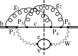
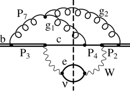
                                           (a) (b)

FIG. 1.: Notation used for the propagators $P_{i}$ in diagrams contributing to semileptonic $b$ decays: examples with two gluons (a) QED-like and (b) with a nonabelian coupling.

         

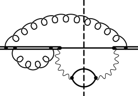
FIG. 2.: The simplest diagram in which the Taylor expansion in $(m_{b}-m_{c})/m_{c}$ leads to spurious divergences and must be supplemented by an eikonal expansion.

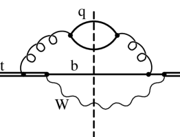
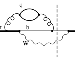
                                           (a) (b)

FIG. 3.: Examples of the light-quark loop corrections to the top quark decay.

REFERENCES

• [1] Particle Data Group, Phys. Rev. D54, 1 (1996).
• [2] M. Shifman, N.Β G. Uraltsev, and A. Vainshtein, Phys. Rev. D51, 2217 (1995), erratum: ibid. D52, 3149 (1995).
• [3] M. Neubert, preprint hep-ph/9702375, to appear in A. Buras and M. Lindner (eds.), Heavy Flavours, 2nd edition, (World Scientific, Singapore).
• [4] A. Czarnecki, Phys. Rev. Lett. 76, 4124 (1996).
• [5] A. Czarnecki and K. Melnikov, hep-ph/9703277, submitted to Nucl. Phys. B (unpublished).
• [6] A. Czarnecki and K. Melnikov, Phys. Rev. Lett. 78, 3630 (1997).
• [7] A. Czarnecki, in New computing techniques in physics research IV, edited by B. Denby and D. Perret-Gallix (World Scientific, Singapore, 1995), pp.Β 319–323, Proceedings of the International Workshop AINHEP 1995, Pisa, Italy.
• [8] V.Β A. Smirnov, Phys. Lett. B394, 205 (1997).
• [9] A. Czarnecki and V.Β A. Smirnov, Phys. Lett. B394, 211 (1997).
• [10] K.Β G. Chetyrkin and F. Tkachov, Nucl. Phys. B192, 159 (1981).
• [11] M. JeΕΌabek and J.Β H. KΓΌhn, Nucl. Phys. B314, 1 (1989).
• [12] A. Czarnecki and S. Davidson, Phys. Rev. D 48, 4183 (1993).
• [13] B.Β H. Smith and M.Β B. Voloshin, Phys. Lett. B340, 176 (1994).
• [14] A. Czarnecki, Acta Phys. Pol. B26, 845 (1995).
• [15] J.Β G. KΓΆrner, K. Melnikov, and O. Yakovlev, Z. Phys. C69, 437 (1996).
• [16] A. Kapustin, Z. Ligeti, M.Β B. Wise, and B. Grinstein, Phys. Lett. B375, 327 (1996).
• [17] A.Β Czarnecki, K.Β Melnikov,Β N.Β G.Β Uraltsev, in preparation.