hep-ph/9706210 FERMILAB–Pub–97/163–T

Saclay–SPhT–T97/54

DTP/97/42

Jet Investigations Using the Radial Moment
W. T. Giele
Fermi National Accelerator Laboratory, P. O. Box 500,
Batavia, IL 60510, U.S.A.

E. W. N.  Glover
Physics Department, University of Durham,
Durham DH1 3LE, England

and

David A. Kosower
Service de Physique Théorique, Centre d’Etudes de Saclay,
F–91191 Gif-sur-Yvette cedex, France

We define the radial moment, $\langle r\rangle$, for jets produced in hadron-hadron collisions. It can be used as a tool for studying, as a function of the jet transverse energy and pseudorapidity, radiation within the jet and the quality of a perturbative description of the jet shape. We also discuss how non-perturbative corrections to the jet transverse energy affect $\langle r\rangle$.

Prospectors for new physics congregrate at the high-energy frontier. Their searches require confronting experimental data with theoretical expectations. Confidence in their claims of new physics presupposes not only a proper comparison of data to theory, but also a solid understanding of systematic uncertainties in both theory and experiment. An interesting case study is the allegation of new physics based on the high-energy tail of the single-jet inclusive transverse energy distribution measured by the CDF and DØ detectors at Fermilab [1, 2]. Data from both experiments agree well with both the theory (EKS [3] for CDF and Jetrad [4, 5, 6] for DØ ) and with each other for jets of transverse energy less than about 200 GeV, while at higher energies the CDF data appear to be somewhat larger than expected (see for example [7]). A genuine rise above theoretical expectations at large transverse energies would be the signal of one of a whole panoply of new physics possibilities. Confidence in such a claim, however, requires that we first rule out more prosaic explanations, such as an uncertainty in the distributions of partons inside the colliding nucleons [8, 9], one of the non-perturbative inputs to the theoretical computation. In order to help resolve the apparent discrepancies between the experiments, and also to clarify puzzling aspects of the cross sections measured at lower energies [11, 12], we feel it is important to examine other observable quantities in the same high transverse-energy events. For example, Ellis, Khoze and Stirling [10] have proposed studying the radiation between jets in order to identify the underlying color structure of the hard scattering.

In this paper, we advocate studying the radiation within a jet, and its use as a diagnostic tool for the quality of the perturbative description of the jet shape as a function of transverse energy. Both CDF [13] and DØ [14] have measured the transverse-energy profile of jets, where the integrated density as a function of the radius $r$ from the jet axis,

$$\Psi(r,E_{T},\eta)=\frac{\int_{0}^{r}\,E_{T}(r^{\prime})dr^{\prime}\frac{d\sigma}{dE_{T}d\eta}}{\int_{0}^{R}\,E_{T}(r^{\prime})dr^{\prime}\frac{d\sigma}{dE_{T}d\eta}}.$$

In terms of particle (tower) $i$ within the jet and lying at a distance $r_{i,{\rm jet}}$ from the jet axis, where,

$$r^{2}_{i,{\rm jet}}=(\Delta\phi_{i,{\rm jet}})^{2}+(\Delta\eta_{i,{\rm jet}})^{2},$$ (1)

we have,

$$\Psi(r,E_{T},\eta)=\frac{\left\langle\sum_{i,r_{i,{\rm jet}}<r}E_{Ti}(r_{i,{\rm jet}})\frac{d\sigma}{dE_{T}d\eta}\right\rangle_{\rm jets}}{\left\langle\sum_{i}E_{Ti}(r_{i,{\rm jet}})\frac{d\sigma}{dE_{T}d\eta}\right\rangle_{\rm jets}}.$$

The summation runs over all particles (towers) in the jet and $\sum_{i}E_{Ti}(r_{i,{\rm jet}})=E_{T{\rm jet}}$. These profiles have also been discussed from the theoretical point of view by Ellis, Kunzst and Soper [15, 16] and more recently by Klasen and Kramer [17].

While one can make a qualitative or semi-quantitative comparison with theoretical predictions, the language of jet profiles does not lend itself readily to the extraction of fundamental quantities, or to identifying possible problems with underlying events or the energy calibration of jets. It would be better to summarize the jet profiles in a small set of numbers, whose variation with $E_{T}$ and $\eta$ can then be mapped more easily. The simplest such number is the radial moment of the transverse energy distribution within the jet, which we shall denote $\langle r\rangle$,

$$\langle r\rangle=\frac{\left\langle\sum_{i}r_{i,{\rm jet}}E_{Ti}(r_{i,{\rm jet}})\frac{d\sigma}{dE_{T}d\eta}\right\rangle_{\rm jets}}{\left\langle\sum_{i}E_{Ti}(r_{i,{\rm jet}})\frac{d\sigma}{dE_{T}d\eta}\right\rangle_{\rm jets}}.$$ (2)

In the central region, $E_{T}\sim E$, and $r\sim\theta$; for massless partons within narrow jets, $rE_{T}$ is then roughly $\theta E\sim|{\bf k}|\sin\theta$, where $\theta$ is the angle between the parton and the jet axis. This quantity is simply the transverse momentum of the parton with respect to the jet axis. The radial moment can thus be understood for narrow jets in the central region as the average transverse momentum with respect to the jet axis, divided by the jet’s $E_{T}$. In the context of two-jet inclusive distributions, the triply-differential distribution $d^{3}\sigma/dE_{T}d\eta_{1}d\eta_{2}$ we have discussed previously [18] extracts as much global information about the event as possible, from the viewpoint of perturbative QCD. The moment $\langle r\rangle$ is independent of this distribution, and its comparison with theoretical predictions may provide us with additional information. As we shall discuss below, the moment is sensitive to the size of the underlying event as well as to the experimental jet algorithm.

The moment vanishes in a lowest-order calculation of jet cross sections, since jets at that order are approximated by lone partons; a next-to-leading order calculation of jet cross sections thus gives the leading non-vanishing calculation of the moment. Using the Jetrad implementation [4, 5, 6] of ${\cal O}(\alpha_{s}^{3})$ parton scattering processes [19], it is straightforward to evaluate $\langle r\rangle$ for an arbitrary jet algorithm. The dependence of the moment on $E_{T}$ using a perturbative implementation of the Snowmass algorithm with $R=0.7$ is displayed in fig. 1. To mimic the DØ acceptance, the jets have been restricted to the central rapidity region, $|\eta|<0.2$. For reference, we use the CTEQ4M parton distribution set together with a renormalization/factorization scale $\mu=0.5E_{T}$.

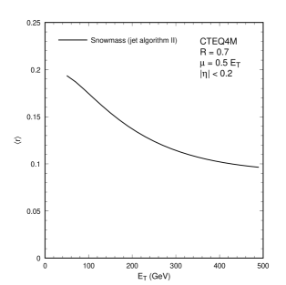
Figure 1: The moment $\langle r\rangle$ as a function of the jet transverse energy at $\sqrt{s}=1800$ GeV using the CTEQ4M parton distributions, for jets with $|\eta|<0.2$ reconstructed using a perturbative implementation of the Snowmass algorithm (jet algorithm II defined in eq. 7) for the jet cone size $R=0.7$. The renormalization and factorization scales have been chosen to be equal to $0.5E_{T}$. These parameters form our baseline choice.

For narrow central jets, we can model the radiation pattern we expect using the collinear approximation to the matrix elements. We find,

$$\langle r\rangle\sim g^{2}(\mu)\int r\frac{dsdz}{16\pi^{2}}\frac{1}{s}P(z)\,,$$ (3)

where $P(z)$ is an Altarelli-Parisi splitting function. The dependence on the hard cross section, including the dependence on the parton distribution functions, disappears; only the dependence on $\alpha_{s}$ remains. With $\theta_{i}$ the angle between the jet axis and parton $i$,

$$s = 2z(1-z)E^{2}(1-\cos(\theta_{1}+\theta_{2}))$$ (4)

$$\sim z(1-z)E^{2}(\theta_{1}+\theta_{2})^{2}.$$

Balancing of transverse momentum within the jet gives the additional relation,

$$z\theta_{1}=(1-z)\theta_{2}.$$

With the change of variables, $r_{1}=z\theta_{1}$, $r_{2}=(1-z)\theta_{2}$, we have,

$$\langle r\rangle\sim\frac{g_{s}^{2}(\mu)}{4\pi^{2}}\left(\int dz\,zP(z)\int d\theta_{1}+\int dz\,(1-z)P(1-z)\int d\theta_{2}\right).$$

The limits in our integral are determined by the clustering in the jet algorithm we are using. At next-to-leading order in perturbation theory, there are two distinct choices for whether or not the two partons will be clustered to form a jet of cone-size $R$, depending on whether the parton-parton or parton-jet distance is constrained to be less than $R$;

$${\rm I}.~{}~{}~{} r_{12}<R,$$ (5)

$${\rm II}.~{}~{}~{} r_{i,{\rm jet}}<R.$$ (6)

In this latter algorithm, two partons with equal transverse energy will combine to form a single jet even if $r_{12}=2R$. In this case, the jet will have all the transverse energy lying on the edge of the jet. It is unlikely that an experimental jet, made up of transverse energy smeared over many calorimeter cells will reconstruct such a jet; it is much more likely to find two (smaller $E_{T}$ jets), with an overlapping region. This is impossible to model accurately at next-to-leading order when at most two partons can merge. However, it is usually [15, 16, 17] approximated by the constraint,

$${\rm III}.~{}~{}~{}r_{i,{\rm jet}}<R\qquad{\rm and}\qquad r_{12}<R_{\rm sep}R,$$ (7)

where $1<R_{\rm sep}<2$. When $R_{\rm sep}=1$, we find jet algorithm ${\rm I}$, while for $R_{\rm sep}=2$ we obtain algorithm ${\rm II}$. Even after choosing the clustering criterion, there still remains a choice of recombination scheme. The most common choice is the Snowmass recombination method [20] originally designed to make semi-analytic theoretical calculations feasible. Since this is a reasonable approximation to the CDF and DØ  recombination schemes in the central region we choose to adopt this scheme for the calculation of $\langle r\rangle$ at ${\cal O}(\alpha_{s}^{3})$.

For the jet cluster algorithm ${\rm III}$, and assuming $\theta_{1}>\theta_{2}$, we have the constraints $\theta_{1}<R$ and $\theta_{1}<(1-z)R_{\rm sep}R$. This translates into the bounds, $\theta_{1}<R$ and $\theta_{2}<zR/(1-z)$ for $z<(R_{\rm sep}-1)/R_{\rm sep}=x$ while $\theta_{1}<(1-z)R_{\rm sep}R$ and for $(R_{\rm sep}-1)/R_{\rm sep}<z<1/2$. Summing over both partons (and including a factor of 2 for the case $\theta_{2}>\theta_{1}$), yields,

$$\langle r\rangle_{{\rm III}} = \frac{\alpha_{s}(\mu)}{\pi}\left(\int_{0}^{x}dz\,zP(z)\int_{0}^{R}d\theta_{1}+\int_{x}^{\frac{1}{2}}dz\,(z)P(z)\int_{0}^{(1-z)R_{\rm sep}R}d\theta_{1}\right.$$ (8)

$$\quad\left.+\int_{x}^{\frac{1}{2}}dz(1-z)P(1-z)\int_{0}^{zR_{\rm sep}R}d\theta_{2}+\int_{0}^{x}dz\,(1-z)P(1-z)\int_{0}^{zR/(1-z)}d\theta_{2}\right)\,$$

$$\equiv \frac{\alpha_{s}(\mu)}{\pi}R{\cal P}^{{\rm III}},$$

There are two possibilities to consider: where the parent parton is (a) a quark or (b) a gluon. Integrating the appropriate splitting functions, we obtain,

$${\cal P}^{{\rm III}}_{gluon} = \frac{(60\ln(R_{\rm sep})+5+60/R_{\rm sep}+10/R_{\rm sep}^{3}-3/R_{\rm sep}^{4}-30/R_{\rm sep}^{2}-21R_{\rm sep})N}{15}$$

$$+\frac{(20-30/R_{\rm sep}+30/R_{\rm sep}^{2}-20/R_{\rm sep}^{3}+6/R_{\rm sep}^{4}-3R_{\rm sep})n_{f}}{30},$$

$${\cal P}^{{\rm III}}_{quark} = \frac{(8\ln(R_{\rm sep})+2+6/R_{\rm sep}-3R_{\rm sep}-2/R_{\rm sep}^{2})(N^{2}-1)}{4N}.$$ (9)

Inserting the numerical values $N=3$ and $n_{f}=5$ and fixing $R_{\rm sep}=1$ we obtain the radial moments for jet cluster criterion ${\rm I}$,

$${\cal P}^{{\rm I}}_{gluon} = \frac{14N+n_{f}}{10}=4.7,$$

$${\cal P}^{{\rm I}}_{quark} = \frac{3(N^{2}-1)}{4N}=2,$$ (10)

while for $R_{\rm sep}=2$ and jet cluster criterion ${\rm II}$, we find,

$${\cal P}^{{\rm II}}_{gluon} = \frac{(192\ln(2)-43)N+7n_{f}}{48}=6.36,$$

$${\cal P}^{{\rm II}}_{quark} = \frac{(16\ln(2)-3)(N^{2}-1)}{8N}=2.70.$$ (11)

As expected, this gives rise to somewhat fatter jets. However, in both cases, ${\cal P}_{gluon}/{\cal P}_{quark}\sim 2.35$ so that the relative fatness of ‘gluon’ and ‘quark’ jets is preserved. Furthermore, ${\cal P}^{{\rm II}}_{gluon}/{\cal P}^{{\rm I}}_{gluon}\sim{\cal P}^{{\rm II}}_{quark}/{\cal P}^{{\rm I}}_{quark}\sim 1.35.$ Other choices for $R_{\rm sep}$ yield values smoothly dispersed between these two extremes but preserving the relative fatness of the types of jets.

As the jet-defining radius $R$ increases, the collinear approximation gets worse, but nonetheless we expect the general features of this simple model to survive: the moment should be roughly a constant times $\alpha_{s}(\mu)$, where $\mu$ is a scale characterizing the jet. In particular, it should be nearly independent of the parton distribution function. However, the parton distributions do play an important role. As we increase the hardness of the scattering we sample different types of jet. The matrix elements for the different subprocesses are (within color factors) rather similar for scattering at $\sim 90^{\circ}$, and the dominant effect is due to the variation of the quark and gluon parton densities with $x$. This is illustrated in fig. 2 where we show the fraction of ‘quark’ and ‘gluon’ jets at $\sqrt{s}=1800$ GeV as a function of the jet transverse energy for the CTEQ4M parton distributions [22]. While ‘gluon’ jets dominate at $E_{T}<120$ GeV, as the quark density functions become more important, the fraction of ‘gluon’ jets diminishes. Different parton distributions give quite different results. In particular, the CTEQ fit to the supposed excess of jets high transverse momentum CTEQ4HJ [22] containing an enhanced gluon at large $x$ generates a larger fraction of ‘gluon’ jets at high $E_{T}$.

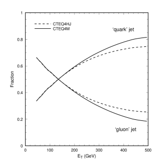
Figure 2: The fraction of ‘quark’ and ‘gluon’ jets for $|\eta|<0.2$ and $\sqrt{s}=1800$ GeV as a function of the jet transverse energy for the CTEQ4M and CTEQ4HJ parton density functions.

This variation of $\langle r\rangle$ with the choice of distribution function set is contrasted in fig. 3 with the relatively greater sensitivity of the inclusive-jet spectrum. To make a fair comparison, we use the CTEQ4 fit with an enhanced gluon at large $x$ that describes the single jet inclusive distribution well at high $E_{T}$, CTEQ4HJ [22], and a ‘normal’ fit by the MRS collaboration [23] with a similar value of $\alpha_{s}(M_{Z})$. The relative insensitivity to parton distribution functions makes this moment a useful tool for measuring the strong coupling constant.

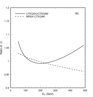
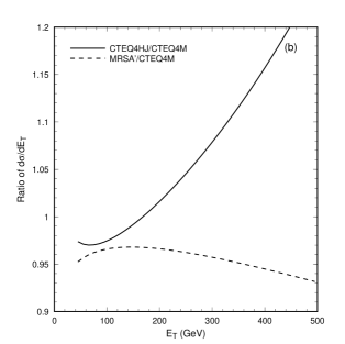
Figure 3: (a) The ratio of $\langle r\rangle$ for the CTEQ4HJ and MRSA^′ $(\alpha_{s}(M_{Z})=0.115)$ distribution sets to that for the CTEQ4M set, as a function of the jet transverse energy. (b) The ratio of the single-jet inclusive cross section computed for the CTEQ4HJ and MRSA^′ $(\alpha_{s}(M_{Z})=0.115)$ distribution sets to that for the CTEQ4M set. In both cases the renormalization and factorization scales are equal to $0.5E_{T}$ and $|\eta|<0.2$ and $R=0.7$.

The radial moment is also somewhat more sensitive to the jet algorithm than the single-jet inclusive cross section, as illustrated in fig. 4 for jet algorithms ${\rm I}$ and ${\rm III}$ with $R=0.7$ and $R_{\rm sep}=1.3$ relative to algorithm ${\rm II}$. Once again, the jets are constrained to lie centrally, $|\eta|<0.2$. We see that both the normalization, and to a lesser extent, the rate of decrease of $\langle r\rangle$ vary more than the single-jet $E_{T}$ spectrum under changes of the jet algorithm.

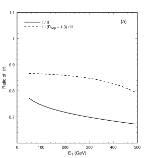
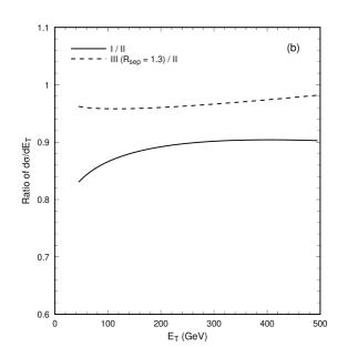
Figure 4: (a) The ratio of $\langle r\rangle$ for the jet algorithms defined in the text as function of the jet transverse energy. (b) The ratio of the single-jet inclusive cross section for the same jet algorithms. In both cases, CTEQ4M parton distributions have been used with renormalization and factorization scales equal to $0.5E_{T}$ and $|\eta|<0.2$ and $R=0.7$.

Of course, the calculations presented here will suffer a significant renormalization-scale dependence, as they are leading-order calculations of the radial moment; a measurement of $\alpha_{s}$ would require a next-to-leading order calculation of this quantity. To estimate the scale uncertainty, we compute the ratio of $\langle r\rangle$ computed with $\mu=0.25E_{T}$ and $\mu=E_{T}$ relative to the same quantity at our reference scale choice $\mu=0.5E_{T}$ for jet clustering algorithm ${\rm II}$. We see in fig. 5, the scale variation is still sizeable and affects the normalization considerably. On the other hand, varying the scale hardly changes the shape.

Armed with the perturbative predictions, we can ask whether the radial moment is sensitive to non-perturbative contributions, either to the jet energy or to the pattern of radiation within the jet. These may arise from various sources, such as power ($1/Q$) corrections to the hard scattering process, spectator interactions, or soft hadrons in the proton/antiproton remnants spilling into the jet cone. Another source of uncertainty is detector-related effects such as the jet energy-scale uncertainty. For example, the debris of the hard scattering tends to form a roughly uniform distribution in pseudorapidity and azimuth. Shower models are used to estimate this underlying event and thereby correct the jet energy. These have been extensively tuned at moderate energies where the data are plentiful. However, if the underlying event was not properly modelled as a function of $E_{T}$, a residual jet energy correction could occur.

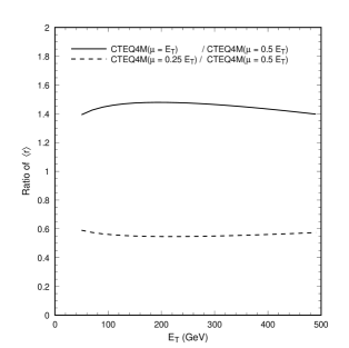
Figure 5: The radial moment $\langle r\rangle$ for renormalization/factorization scale $\mu=\lambda E_{T}$ relative to that for $\mu=E_{T}$ for central jets, $|\eta|<0.2$ using the cluster criterion ${\rm II}$ and the Snowmass recombination procedure. The solid (dashed) lines shown the change for $\lambda=0.5$ (2.0). In all cases, the MRSA^′ parton distributions have been utilized.

In the simplest string-like hadronization model [24], we expect to find a contribution of order $C\sim 1$ GeV to the transverse momentum $p_{t}$ with respect to the jet axis in a central jet. Since the average $p_{t}$ is roughly $\langle r\rangle E_{T}$, this implies a non-perturbative correction of order $C/(\langle r\rangle E_{T})$. We expect the corrections to the radial moment to be of the same order. The underlying event is also expected to contribute a $1/Q$ correction. If we assume that the energy is deposited uniformly, we expect a contribution to $\langle r\rangle$ of order

$$\frac{\pi E_{u}}{E_{T}}\left(\frac{2R}{3}-\langle r\rangle\right)\,,$$ (12)

where $E_{u}$ is the underlying event transverse energy density (per unit rapidity per radian). In minimum-bias events, this is $\sim 0.55\pm 0.1$ GeV according to ref. [25]. Some of this is subtracted as part of the experimental analysis. Since $\langle r\rangle$ varies from $\sim 0.25$ to $\sim 0.07$, this correction should anyway be much smaller than that due to hadronization.

A determination of $\alpha_{s}$, which is less sensitive to the parton distributions than other determinations at hadron colliders, and the possible identification of detector and/or physics based non-perturbative contributions are both interesting to pursue. This gives the jet-shape analysis a well defined physics goal, and motivates the determination of jet shapes over a large range of transverse energies. While a sensible analysis requires at least the next-to-leading order contributions to the jet shape, we can already confront the published CDF and DØ data on the quantity $\Psi(r,E_{T},\eta)$ defined in eq. 1 with the leading-order calculations. This allows us to explore the potential utility of this measurement, and indicate expected uncertainties and problems.

The current published data on the jet shape from both CDF and DØ are very limited. The CDF collaboration published results based on 4.2 pb^-1 with only three bins of transverse energy, while DØ used 13 pb^-1 with four bins in transverse energy. A full analysis of current data would include on the order of 100 pb^-1 from each collaboration, preferably using the same binning in $E_{T}$ as used in the one-jet inclusive transverse-energy distribution. Substantial experimental improvements to the results presented here are thus possible. In addition, we expect the next-to-leading order theoretical corrections to be available soon. The latter will enable us to extract the next-to-leading order $\alpha_{s}$ and determine the uncertainty on the radial moment, and will be crucial in understanding the magnitude of non-perturbative effects.

We must first determine the radial moment $\langle r\rangle$ from the published results for the quantity $\Psi$. In an analysis along the lines suggested in this paper one would of course determine the radial moment as a function of transverse energy directly from the data without resorting to extracting the explicit shapes. This would reduce the experimental uncertainties significantly, especially the systematic uncertainties. For now, we have to reconstruct the radial moment from the quantity $\Psi$:

$$\langle r(E_{T},\eta)\rangle=\int_{0}^{R}r\frac{\partial\Psi(r,E_{T},\eta)}{\partial r}d\,r\ .$$ (13)

The values of $\langle r\rangle$ extracted from the published data are shown in Table 1. Both experiments use $R=1$, but the allowed range of rapidity for the jets is different. CDF consider jets in the range $0.1<|\eta|<0.7$ while DØ have a tighter restiction, $|\eta|<0.2$.

$E_{T}$-bin (GeV)	$\langle E_{T}\rangle$ (GeV)	experiment	$\langle r\rangle|_{\mbox{experiment}}$
40–60	45	CDF	0.31 $\pm$ 0.02
45–70	53	DØ	0.29 $\pm$ 0.01
65–90	75	CDF	0.24 $\pm$ 0.02
70–105	81	DØ	0.23 $\pm$ 0.01
95–120	100	CDF	0.22 $\pm$ 0.02
105–140	118	DØ	0.19 $\pm$ 0.01
140–900	166	DØ	0.17 $\pm$ 0.01

Table 1: The DØ and CDF experimental results for $\langle r\rangle$ extracted from the published jet shapes.

For the theoretical prediction, we could repeat the experimental extraction, by first determining $\Psi$ using the same binning as the experiments and extract $\langle r\rangle$ from this quantity. This will simulate any effects on $\langle r\rangle$ due to binning and functional parametrization. However, these effects are in practice small and instead we determine $\langle r\rangle$ directly as was done in fig. 1, For the theoretical prediction, we use the CTEQ4M parton distribution set, with $\alpha_{s}(M_{Z})=0.116$. The renormalization and factorization scales were chosen to be half the jet transverse energy. To match the experimental cuts, we use $R=1$ and $R_{\rm sep}=1.3$ was used to simulate the jet splitting and merging effects, which are not modelled at this order in perturbation theory.

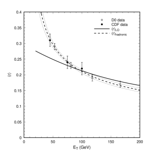
Figure 6: The extracted values for $\langle r\rangle$ for DØ (open circles) and CDF (solid circles). The theoretical prediction for $|\eta|<0.2$, CT 4M parton distributions, $R=1$ and $R_{\rm sep}=1.3$ and $\mu=0.5E_{T}$ is shown as a solid line. The fitted theoretical result with an additional non-perturbative component as described in eq. 14 and $C=1.09$ and $K=0.56$ is given by the dashed line; the dotted lines indicate the 1$\sigma$ variations in the fit.

The extracted experimental values for $\langle r\rangle$ are shown in fig. 6 along with the theoretical prediction as a function of $E_{T}$. We see that the CDF and DØ points are compatible with each other (despite the fact that the experiments use slightly different rapidity cuts on the jet). On the other hand, the leading-order predictions cannot describe the data, as its $E_{T}$ dependence is substantially different from that of the data. As was already demonstrated in fig. 5 while the normalization of the leading-order prediction has a strong dependence on the choice of the renormalization/factorization scale, the shape is mostly independent of this choice. Thus, although we assume that higher-order corrections will modify the normalization, it is reasonable to assume that they will not modify the shape substantially.

This suggests that the explanation of the shape of the data lies in hadronization effects (i.e. power corrections). To test this hypothesis, we will assume that the perturbative prediction $\langle r\rangle_{\it perturbative}$ is a constant $K$ times the leading-order prediction $\langle r\rangle_{LO}$. We model the hadronization effects as described earlier, so that

$$\langle r\rangle_{\it hadronic} = \langle r\rangle_{\it partonic}+\frac{C}{\langle r\rangle_{\it partonic}E_{T}^{\rm jet}}$$ (14)

$$= K\langle r\rangle_{\rm LO}+\frac{C}{K\langle r\rangle_{\rm LO}E_{T}^{\rm jet}}$$

where the non-perturbative scale $C$ should be close to 1 GeV. We then perform a fit of this model to the data varying both the $K$-factor and the hadronization scale $C$. The fit result with a hadronization scale $C=1.09\pm 0.05$ GeV and $K=0.56\pm 0.11$ is shown in fig. 6. Other choices of renormalization scale give roughly the same value of $C$. This is not surprising because $C$ changes the shape of the curve while the renormalization scale affects primarily the normalization. This shows that the above model might explain the observed differences between the leading-order predictions and the data. The $K$-factor has a strong dependence on the renormalization scale, as expected.

Only a next-to-leading order calculation of $\langle r\rangle$ can confirm that power corrections, rather than higher-order corrections, are responsible for the observed behavior of the data. Such a calculation requires the one-loop five-parton matrix elements [26] as well as the six-parton tree-level ones [27], all of which are available in the literature. With such NLO predictions, one could extract both an NLO $\alpha_{s}$ (sensitive to the normalization and the high-$E_{T}$ dependence of $\langle r\rangle$) and the hadronization scale $C$ (sensitive to the low-$E_{T}$ dependence of $\langle r\rangle$). In order to perform such an extraction, however, we need a much more extensive measurement of the $E_{T}$ dependence of $\langle r\rangle$. With current CDF and DØ data sets, it should be possible to cover a much larger $E_{T}^{\rm jet}$ range (both lower and higher than the current published results) with a finer binning. This would enable a study of power corrections and their impact on the uncertainty in an extracted $\alpha_{s}$.

A few remarks are in order. The current iterative cone algorithm will be rather problematic in such an NLO calculation (these are the problems one would encounter in a next-to-next-to-leading order calculation of jet differential cross sections). For the studies performed in this paper, we used a phenomenological parameter $R_{\rm sep}=1.3$ to model jet splitting and merging. At the next order in perturbation theory, one should either abandon this parameter (relying on the theory to model jet splitting and merging), or else one must introduce an additional $R_{\rm sep}^{\rm NLO}$. For the purposes considered here, $R_{\rm sep}$ is anyway an especially suspect parameter because it is purely phenomenological and may well be $E_{T}$ dependent [17]. Indeed, as we have seen in this paper, jets get narrower as their energy increases. With this observation one could argue that $R_{\rm sep}$ should in fact decrease with increasing energy of the jet. A simple way out of this morass is to use the $K_{T}$ jet algorithm [28, 16]. It has good perturbative behaviour and no additional phenomenological parameters are needed.

The analysis discussed in the present paper suggests that it should be possible to use the hadronic dijet system to determine both $\alpha_{s}$ and the proton’s gluon distribution with great accuracy. The gluon distribution would be determined by the triply-differential distribution, and, once the next-to-leading order calculations are available, $\alpha_{s}$ would be determined by the radial moment. Only the quark distributions would be taken from deeply-inelastic scattering data. Use of the full current data set would allow a much finer jet $E_{T}$ binning as well as much higher jet $E_{T}$ to be used, reducing the experimental uncertainties on $\langle r\rangle$ significantly reduced, and thereby reducing the significance of power corrections. If the higher-order perturbative corrections are also small, as suggested by the phenomenological study performed in this paper, the theoretical uncertainties should be competitively small as well. We may also expect the high-$E_{T}$ jet profiles to be especially sensitive to jet production from new physics, and thus the $E_{T}$ dependence of the radial moment should be a good probe of the presence (or absence) of physics beyond the standard model.

References

- [1] F. Abe et al, CDF Collaboration, Phys. Rev. Lett. 77, 438 (1996).
- [2] G. C. Blazey for the DØ Collaboration, Proceedings 31st Rencontres de Moriond: ”QCD and High-energy Hadronic Interactions”, Les Arcs, France, (1996), p 155.
- [3] S.D. Ellis, Z. Kunszt and D.E. Soper, Phys. Rev. Lett. 62, 726 (1989); Phys. Rev. D40, 2188 (1989); Phys. Rev. Lett. 64, 2121 (1990).
- [4] W. T. Giele, E. W. N. Glover, and D. A. Kosower, Phys. Rev. Lett. 73:2019 (1994) [hep-ph/9403347]
- [5] W. T. Giele, E. W. N. Glover and D. A. Kosower, Nucl. Phys. B403, 633 (1993).
- [6] W. T. Giele and E. W. N. Glover, Phys. Rev. D46, 1980 (1992).
- [7] H. L. Lai and W.-K. Tung, ‘Comparison of CDF and DØ Inclusive Jet Cross Sections’, hep-ph/9605269.
- [8] E. W. N. Glover, A. D. Martin, R. G. Roberts and W. J. Stirling, Phys. Lett. B381, 353 (1996).
- [9] J. Huston et al, CTEQ Collaboration, Phys. Rev. Lett. 77, 444 (1996). [hep-ph/9511386]
- [10] J. Ellis, V.A. Khoze and W.J. Stirling, ‘Hadronic Antenna Patterns to Distinguish Production Mechanisms for Large- Jets’, hep-ph/9608486.
- [11] T. Devlin for the CDF Collaboration, XXVIIIth International Conference on High Energy Physics, Warsaw, Poland, July 1996.
- [12] J. Krane for the D0 Collaboration, DPF96; Annual Divisional Meeting of the Division of Particles and Fields of the American Physical Society, Minnesota, U.S.A., August 1996.
- [13] F. Abe et al, CDF Collaboration, Phys. Rev. Lett. 70, 713 (1993).
- [14] S. Abachi et al, DØ Collaboration, Phys. Lett. B357, 500 (1995).
- [15] S.D. Ellis, Z. Kunszt and D.E. Soper, Phys. Rev. Lett. 69, 3615 (1992).
- [16] S.D. Ellis and D.E. Soper, Phys. Rev. D48, 3160 (1993).
- [17] M. Klasen and G. Kramer, ‘Jet Shapes in and Collisons in NLO QCD’, hep-ph/9701247.
- [18] W. T. Giele, E. W. N. Glover, and D. A. Kosower, Phys. Rev. D52:1486 (1995) [hep-ph/9412338]
- [19] R. K. Ellis and J. Sexton, Nucl. Phys. B269, 445 (1986).
- [20] S. D. Ellis, J. Huth, N. Wainer, K. Meier, N. Hadley, D. Soper, and M. Greco, in Research Directions for the Decade, Proceedings of the Summer Study, Snowmass, Colorado, 1990, ed. E. L. Berger (World Scientific, Singapore, 1992), p134.
- [21] E.W.N. Glover and D.A. Kosower, Phys. Lett. 367B, 369 (1996).
- [22] H.L. Lai et al, CTEQ Collaboration, Phys. Rev. D55, 1280 (1997). [hep-ph/9606399]
- [23] A. D. Martin, R. G. Roberts and W. J. Stirling, Phys. Rev. D50, 6734 (1994); Phys. Lett. B354, 155 (1995).
-
[24]
R. P. Feynman, Photon-Hadron Interactions,
W. A. Benjamin (New York, 1972);
B. R. Webber, Lectures at the Summer School on Hadronic Aspects of Collider Physics, Zuoz, Switzerland, August 1994 [hep-ph/9411384]. - [25] B.K. Abbott, Ph.D. thesis, Purdue University, UMI-95-23307 (1994).
-
[26]
Z. Bern, L. Dixon, and D. A. Kosower,
Phys. Rev. Lett. 70:2677 (1993) [hep-ph/9302280];
Z. Bern, L. Dixon, and D. A. Kosower, Nucl. Phys. B437:259 (1995) [hep-ph/9409393];
Z. Kunszt, A. Signer, Z. Trocsanyi, Phys. Lett. B336:529 (1994) [hep-ph/9405386]. - [27] see M. L. Mangano and S.J. Parke, Phys. Reports, 200, 301 (1991) and references therein.
- [28] Yu.L. Dokshitzer, Contribution to the Workshop on Jets at LEP and HERA, J. Phys. G17 (1991) 1441; S. Catani, Yu.L. Dokshitzer, M.H. Seymour and B.R.Webber, Nucl. Phys. B406, 187 (1993).