Nonequilibrium inflaton dynamics and reheating:
Back reaction of parametric particle creation and curved spacetime effects

Abstract

We present a detailed and systematic analysis of the nonperturbative, nonequilibrium dynamics of a quantum field in the reheating phase of inflationary cosmology, including full back reactions of the quantum field on the curved spacetime, as well as the fluctuations on the mean field. We use the O$(N)$ field theory with unbroken symmetry in a spatially flat Friedmann-Robertson-Walker (FRW) universe to study the dynamics of the inflaton in the post-inflation, preheating stage. Oscillations of the inflaton’s zero mode induce parametric amplification of quantum fluctuations, resulting in a rapid transfer of energy to the inhomogeneous modes of the inflaton field. The large-amplitude oscillations of the mean field, as well as stimulated emission effects require a nonperturbative formulation of the quantum dynamics, while the nonequilibrium evolution requires a statistical field theory treatment. We adopt the coupled nonperturbative equations for the mean field and variance derived in a preceding paper [1] by means of a two-particle-irreducible (2PI), closed-time-path (CTP) effective action for curved spacetimes while specialized to a dynamical FRW background, up to leading order in the $1/N$ expansion. Adiabatic regularization is employed to yield a covariantly conserved, renormalized energy-momentum tensor. The renormalized dynamical equations are evolved numerically from initial data which are generic to the end state of slow roll in many inflationary cosmological scenarios. The initial conditions consist of a large-amplitude, quasiclassical, oscillating mean field $\langle\Phi\rangle$ with variance $\langle\Phi^{2}\rangle-\langle\Phi\rangle^{2}$ around the de Sitter-invariant vacuum. We find that for sufficiently large initial mean-field amplitudes $\gtrsim\text{$M_{\text{{P}}}$}/300$ (where $M_{\text{{P}}}$ is the Planck mass) in this model, the parametric resonance effect alone (in a collisionless approximation) is not an efficient means to “preheat” the quantum field. For small initial mean-field amplitude, damping of the mean field via parametric amplification of quantum fluctuations is seen to occur, and in this case can be adequately described by prior analytic studies with approximations based on field theory in Minkowski spacetime. Our results indicate that the self-consistent dynamics of spacetime plays an important role in determining the physics of the post-inflationary Universe. This study calls into question the validity of general claims made without full consideration of the self-consistent dynamics of spacetime and quantum fields.

I Introduction and summary

The inflationary Universe [2, 3, 4, 5, 6, 7, 8, 9, 10, 11, 12, 13] has for over a decade been the new paradigm for addressing many basic issues in cosmology such as the flatness-entropy problem, the horizon-homogeneity problem, and the fluctuation-structure formation problem. The linkage between observations, especially those from the recent Cosmic Background Explorer (COBE) data, and theory, based on grand unified theories (GUT’s) and Friedmann-Robertson-Walker– (FRW–)de Sitter models, has been pursued in earnest, but most theoretical discussions to date are largely phenomenological and somewhat utilitarian in nature [14, 15]. This lack of rigor and precision is understandable for at least two reasons: the precise physical conditions between the Planck and GUT scales (when the most cosmologically significant inflationary evolutions are believed to have taken place) have not been clearly understood, and the theoretical framework for the treatment of processes affecting the inception and completion of inflation were not well developed. As stressed by one of us earlier [16, 17], the important physical processes which can determine whether inflation can occur, sustain, and finish with the necessary features are affected by at least three aspects: the geometry, topology, and dynamics of the spacetime [18], the quantum field theory aspects pertaining to the analysis of infrared behavior, and the statistical mechanical aspects pertaining to nonequilibrium processes. These quantum and statistical processes include phase transition, particle creation, entropy generation, fluctuation or stochastic dynamics, and structure formation [19, 20]. Most of these invoke the quantum field and statistical mechanical aspects, and for processes occurring at the Planck scale (which are instrumental in starting certain models of inflation, such as proposed in [6, 21, 22]), also the geometry and topology of spacetime. Two important problems involving field theory in curved spacetime [18], namely, the back reaction of cosmological particle creation [23, 24, 25, 26, 27] on the structure and dynamics of spacetimes [21, 26, 28, 29, 30, 31, 32, 33, 34, 35], and the effects of geometry and topology of spacetime on cosmological phase transitions [17, 22, 36, 37, 38, 39], were investigated systematically and comprehensively in the 1970s and 1980s. The statistical mechanical aspect has not been considered with equal mastery.

The statistical mechanical aspect enters into all three stages of inflationary cosmology: (i) At the inception: What conditions would be most conducive to starting inflation? Do there exist metastable states for the Higgs boson field which can generate inflation [40]? Can thermal or quantum fluctuations assist the inflaton in hopping or tunneling out of the potential barrier in the spinodal or nucleation pictures? Most depictions so far have been based on the finite temperature effective potential, which assumes an unrealistic equilibrium condition and a constant background field. However, when asking such questions in critical dynamics one should be using a Langevin or Fokker-Planck equation (a generalized time-dependent Landau-Ginzberg equation [41]) incorporating dynamic dissipation and intrinsic noise consistently. (ii) During inflation, the dynamics of the inflaton field can be more easily understood in terms of a Kadanoff-Migdal exponential scaling transform [42]. The reason why the inflaton evolves as a classical stochastic field [43, 44, 45] at late times involves the process of decoherence, caused by noise and fluctuations from environmental fields [46]; this necessitates statistical mechanical considerations. The evolution of the classical density contrast (containing the seedings of structures) from quantum fluctuations of the inflaton also requires both quantum and stochastic field theory considerations [47, 48, 49, 50, 51, 52, 53, 54, 55, 56]. (iii) In the reheating epoch, particle creation induces dissipation of the inflaton field, and the interaction of quantum fields is the source for reheating the Universe. This last epoch is the focus of much recent work, as we shall detail below.

The construction of a viable theoretical framework for treating quantum statistical processes in the early Universe has been the aim of research of one of us for the past decade (for a review, see [57]). This framework has now been successfully established, and its application to the problems mentioned above has just begun. The cornerstones are the Schwinger-Keldysh closed-time-path (CTP) [58, 59, 60, 61, 62, 63, 64, 65, 66, 67, 68, 69, 70] effective action and the Feynman-Vernon influence functional [71, 72, 73, 74, 75, 76, 77] formalisms. They are useful for treating particle creation back reaction [68, 70], fluctuation or noise, and dissipation or entropy problems [54, 55, 77]. Other essential ingredients include the Wigner function [78, 79], the $n$-particle-irreducible ($n$PI) effective action [80, 38, 69, 1], and the correlation hierarchy [81, 82] for treating kinetic theory processes [69, 83] and phase transition problems [84, 55]. In this and three following papers we apply these techniques to the problems of inflaton dissipation due to parametric particle creation [85, 86] and reheating due to particle interaction [87] (in the third epoch depicted above). In parallel, these newly developed methods in statistical field theory are now being applied to derive the classical stochastic dynamics of the inflaton (in the second epoch) [46], and the statistical field theory of spinodal decomposition (in the first epoch) [41].

A Background and issues

All inflationary cosmologies share the feature of a period of cosmic expansion driven by a nearly constant vacuum energy density $\rho$ (a “vacuum-dominated” era with effective equation of state, $p=-\rho$): In a Friedmann-Robertson-Walker (FRW) spacetime, the scale factor expands exponentially in cosmic time, resulting in extreme redshifting of the energy density of all other forms of matter and fields. As long as the interaction time scale of any physical process involving given fields is longer than the cosmic expansion time $H^{-1}$, the fields will remain in disequilibrium. This condition can prevail in all three stages of inflation, and one should use a fully nonequilibrium, nonperturbative treatment of the dynamics of the inflation field. The physics of the reheating epoch is important because it directly determines several important cosmological parameters which are relevant to later evolution of the Universe, and in principle verifiable by observational data. For example, the reheating temperature is a vital link between the inflationary Universe scenario and GUT scale baryogenesis [88].

It is generally believed that at the end of inflation, the state of the inflaton field can be approximately described by a condensate of zero-momentum particles undergoing coherent quasioscillations about the true minimum of the effective potential [11, 12, 89]. The reheating problem involves describing the processes by which the many light fields coupled to the inflaton become populated with quanta, and eventually thermalize. It is commonly believed that if the fields interact sufficiently rapidly and strongly, the Universe thermalizes and turns into the radiation-dominated condition described by the standard Friedmann solution, but this has not been proven satisfactorily.

There has been a great deal of work over the past 15 years on the reheating problem, and in attempting to understand reheating, a wealth of interesting physics has been revealed (see, e.g., [90]). To date, the work on particle production during reheating largely follows two distinct approaches, each pursued in two stages.

In the first stage of work on the reheating problem (group 1A, [91, 92, 93, 94]), time-dependent perturbation theory was used to compute the rate of particle production into light fields (usually fermions) coupled to the inflaton. Particle production rates were computed in flat space assuming an eternally sinusoidally oscillating inflaton field. The inflaton evolution in FRW spacetime was modeled with a phenomenological c-number equation involving the Hubble parameter $H$ and the classical inflaton amplitude $\phi$,

$$\frac{d^{2}\phi}{dt^{2}}+m^{2}\phi+(\Gamma+3H)\frac{d\phi}{dt}=0,$$ (1)

where $\Gamma$, given by the imaginary part of the self-energy of $\phi$, is the total perturbative decay rate. Bose enhancement of particle production into the spatial Fourier modes of the inflaton fluctuation field $\varphi$ (and light Bose fields coupled to the inflaton) was not taken into account.

In the second stage of this first approach to the reheating problem (group 1B, [95, 96, 97, 98]) Eq. (1) was still utilized to model the mean-field dynamics, but with $\Gamma$ computed beyond first-order in perturbation theory. In the work of Shtanov, Traschen, and Brandenberger [96] and Kofman, Linde, and Starobinsky (KLS) [95], $\Gamma$ was computed for a real self-interacting scalar inflaton field $\phi$ which was both Yukawa-coupled to a spinor field $\psi$, and bi-quadratically coupled to a scalar field $\chi$ (KLS studied both the $\phi\rightarrow-\phi$ symmetry-breaking and unbroken symmetry cases). From the one-loop equations for the quantum modes of the $\chi$, $\varphi$, and $\psi$ fields (in which the mean field $\hat{\phi}$ appears quadratically as an effective mass), approximate expressions for the growth rate of occupation numbers were derived, assuming a quasi-oscillatory mean field $\hat{\phi}$. For bosonic decay-product fields, it was found that first-order time-dependent perturbation theory drastically underestimates the particle production rate for modes which are in an instability band (due to parametric resonance). Parametric amplification of quantum fluctuations in Bose decay-product fields can result in rapid out-of-equilibrium transfer of energy from the inflaton mean field to the (spatially) inhomogeneous inflaton modes and light Bose fields coupled to the inflaton. This phenomenon was called preheating by KLS. It has been suggested that exponential growth of quantum fluctuations can in some cases lead to out-of-equilibrium (nonthermal) symmetry restoration in the “new” inflation models with a spontaneously broken symmetry [99, 100]. (See, however, the work of Boyanovsky et al., which reached a different conclusion on the possibility of nonequilibrium symmetry restoration [101].) This may have interesting implications for baryogenesis, defect formation, and generation of primordial density perturbations [90, 95, 100].

In both stages of this first approach, the back reaction of the variance of the inflaton on the mean-field dynamics, and of the variance on the quantum mode functions, were not treated self-consistently. The effect of spacetime dynamics was either excluded entirely, or not included self-consistently using the semiclassical Einstein equation. Due to the potentially large initial inflaton amplitude at the onset of reheating, particularly in the case of chaotic inflation [12], the effect of cosmic expansion on quantum particle production needs to be included. Since the mean field and variance (mean-squared fluctuations) are coupled, the back reaction of particle production on the mean-field dynamics must be accounted for in a self-consistent manner.

In the decade before the advent of inflationary cosmology, there was active research on quantum processes in curved spacetimes. An important class of problems is vacuum particle creation [23, 24, 25, 26, 27] and its effect on the dynamics and structure of the early Universe [26, 28, 29, 30, 31, 32, 33, 34, 35] at the Planck time. The effect of spacetime dynamics and the importance of parametric amplification on cosmological particle creation were realized very early [23, 25, 27]. Most of the effort in the latter part of the 1970s was focused on obtaining both a regularized energy-momentum tensor and a viable formalism for the treatment of back reaction effects. The wisdom gained from work in that period before the inflationary cosmology program was initiated is particularly relevant to the reheating problem. Simply put, for obtaining a finite energy-momentum tensor for a quantum field in a cosmological spacetime, the adiabatic [27, 102, 103, 104] and dimensional [105] regularization methods are the most useful. For studying the back reaction of particle creation, the Schwinger-Keldysh (CTP, “in-in”) effective action formalism [58, 60, 64, 65, 66, 67, 68, 70] is more appropriate than the usual Schwinger-DeWitt (“in-out”) method [106, 107].

The second approach to the post-inflationary reheating problem is built upon the body of earlier work on cosmological particle creation. Following the application of closed-time-path techniques to nonequilibrium relativistic field theory problems [68, 69], several authors (which we call group 2A) derived perturbative mean-field equations for a scalar inflaton with cubic [70] and quartic [108] self-couplings, as well as for a scalar inflaton Yukawa-coupled to fermions [109]. The closed-time-path method yields a real and causal mean-field equation with back reaction from quantum particle creation taken into account. For the case of Bose particle production, perturbation theory in the coupling constant is known to break down for sufficiently large occupation numbers, which occurs on the time scale $\tau_{1}$ for parametric resonance effects to become important [110, 111]. It is, therefore, necessary to employ nonperturbative techniques in order to study reheating in most inflationary models.

The second stage of work in this second approach to the reheating problem used the closed-time-path method to derive self-consistent mean-field equations for an inflaton coupled to lighter quantum fields (group 2B, [112, 113, 114, 115, 116, 117, 118]). In the first of these studies [112, 113, 114, 115], the coupled one-loop mean-field and mode-function equations were solved numerically in Minkowski space, implicitly carrying out an ad hoc nonperturbative resummation in $\hbar$. In the one-loop equations, the variances for the inflaton $\langle\varphi^{2}\rangle$ and light Bose fields $\langle\chi^{2}\rangle$ do not back-react on the mode functions directly. However, mean-field equations were derived for an O$(N)$-invariant linear $\sigma$ model (with a $\lambda\Phi^{4}$ self-interaction) at leading order in the large-$N$ approximation by Boyanovsky et al. [110]. In this approximation, the variance does back-react on the quantum mode functions. At leading order in the $1/N$ expansion, the unbroken symmetry dynamical equations for the quartic O$(N)$ model are formally similar to the dynamical equations for a single $\lambda\Phi^{4}$ field theory in the time-dependent Hartree-Fock approximation [80]. The nonequilibrium dynamics of the quartically self-interacting O$(N)$ field theory in Minkowski space has been numerically studied at leading order in the $1/N$ expansion in both the unbroken symmetry [101, 110, 119] and symmetry-broken [101, 110, 120] cases. Some analytic work has been done on the self-consistent Hartree-Fock mean-field equations for a quartic scalar field in Minkowski space [111]. In addition, the Hartree-Fock equations for a $\lambda\Phi^{4}$ field in the slow-roll regime have been studied numerically in Minkowski space [121] and in FRW spacetime [122]. However, the effect of spacetime dynamics on reheating in the O$(N)$ field theory has not (to our knowledge) been studied using the coupled, self-consistent semiclassical Einstein equation and matter-field dynamical equations, though some simple analytic work has been done on curvature effects in reheating [97, 116]. The semiclassical equations for one-loop reheating in FRW spacetime were derived in [117]. The $\phi^{2}\chi^{2}$ theory has been studied in FRW spacetime by [54, 118, 123]. In addition, numerical work has been done on symmetry-breaking phase transitions in both a $\lambda\Phi^{4}$ scalar field in de Sitter spacetime [124], and an O$(N)$ theory in FRW spacetime [125, 126]. The group 2B studies represent the state of the art on the preheating problem.

B Our work – how it differs from others

In the present work we study the nonperturbative, out-of-equilibrium dynamics of a minimally coupled scalar O$(N)$ field theory (with quartic self-interaction) in a spatially flat FRW universe whose dynamics is given self-consistently by the semiclassical Einstein equation. The purpose of this study is to understand the preheating period in inflationary cosmology, with particular emphasis on the effect of spacetime dynamics on the phenomenon of particle production via parametric amplification of quantum fluctuations. Of primary interest is obtaining the dynamics of the inflaton (including back reaction from created particles) using rigorous methods of nonequilibrium field theory in curved spacetime [69]. We have chosen to focus in this paper on parametric amplification of quantum fluctuations because this phenomenon can be the dominant effect in the preheating stage of unbroken symmetry inflationary scenarios, among which the chaotic inflation scenarios most directly necessitate (through initial conditions) considerations of Planck-scale physics. “New” inflationary scenarios which involve a spontaneously broken symmetry often contain additional subtleties (e.g., infrared divergences, spinodal instabilities), and are the subject of ongoing investigation [41, 86]. The results of our work are, therefore, particularly relevant to chaotic inflation scenarios [127]. The additional interactions which should be included to treat the broken-symmetry case are discussed in [1].

In the preceding paper [1] we have derived the evolution equations for the mean field $\langle\Phi_{\text{{H}}}\rangle$ (subscript H denotes the Heisenberg field operator) and mean-squared fluctuations (variance) $\langle\Phi_{\text{{H}}}^{2}\rangle-\langle\Phi_{\text{{H}}}\rangle^{2}$ using the closed-time-path (CTP), two-particle-irreducible (2PI) effective action [80] in a fully covariant form. Here we use these results for the case of spatially flat FRW spacetime. The quantum state for the field theory (in the case of FRW spacetime) consists of a coherent state for the spatially homogeneous field mode, and the adiabatic vacuum state for the spatially inhomogeneous modes. At conformal past infinity, the spacetime is assumed to be asymptotically de Sitter, and the mean field is chosen to be asymptotically constant.

In this paper we study the O$(N)$ field theory using the $1/N$ expansion, which yields nonperturbative dynamics in the regime of strong mean field. This is particularly important for chaotic inflation scenarios [6], in which the inflaton mean-field amplitude can be as large as $\text{$M_{\text{{P}}}$}/3$ at the end of the slow-roll period [12, 128]. Treatments of the reheating problem which rely on time-dependent perturbation theory do not apply to such cases where the inflaton undergoes large-amplitude oscillations, in contrast with nonperturbative methods such as large $N$.

We now summarize the principal distinctions between our work and previous treatments of preheating in inflationary cosmology. Our work improves on the group 1A methodology by including parametric resonance effects. As it is based on first-order, time-dependent perturbation theory, the group 1A approach cannot correctly describe the inflaton dynamics with large initial mean-field amplitude. In addition, our work improves on both the group 1A and group 1B studies by including the effect of back reaction from quantum particle creation on both the mean field and the inhomogeneous modes. We are treating the inflaton dynamics from first principles, without assuming a phenomenological equation (with a damping term $\Gamma\dot{\phi}$ put in by hand) for the mean field. In our approach the damping of the mean field is due to back reaction from quantum particle production in the self-consistent equations for the mean field and its variance. In contrast, the analytic results of the group 1A and 1B work are based on the assumption of either large-amplitude mean-field oscillations ($\lambda\text{$\hat{\phi}$}^{2}/2\gg m^{2}$) or harmonic oscillations ($m^{2}\gg\text{$\hat{\phi}$}^{2}/2$), and, therefore, cannot describe the interesting case of inflaton dynamics in which neither term dominates the tree-level effective mass, i.e., $m^{2}\sim\lambda\text{$\hat{\phi}$}^{2}$. Furthermore, our work improves on group 1A, group 1B, and group 2A in that the closed-time-path effective action is computed in curved spacetime without assuming that $H^{-1}\gg\tau_{0}$ (where $\tau_{0}$ is the period of mean-field oscillations). In our work, the dynamics of the two-point function (which reflects quantum particle production) is formulated in curved spacetime assuming only that semiclassical gravity is valid, i.e., $\text{$M_{\text{{P}}}$}\gg H$.

Most significantly, our work improves on all the previous treatments in that it includes curved spacetime effects systematically using the coupled, self-consistent semiclassical Einstein equation and matter field equations. Among the group 2B studies of preheating dynamics, inflaton dynamics has been studied primarily in fixed background spacetimes: Minkowski space [101, 110], de Sitter space [124, 126, 129], and in radiation-dominated, spatially flat FRW spacetime [126]. In the present work, the spacetime is dynamical, with the renormalized trace of the semiclassical Einstein equation governing the dynamics of the scale factor $a$. This permits quantitative study of the transition of the spacetime from the (slow-roll) period of vacuum-dominated expansion to the radiation-dominated (“standard”) FRW cosmology. In particular, our method yields the spacetime dynamics naturally, without making reference to an “effective Hubble constant” (which has been used in calculations on a fixed background spacetime [129]).

With additional couplings (see [1]), our method may also be used to study preheating in “new” inflationary scenarios [5]. In new inflation, the vacuum-dominated expansion of the Universe is typically driven by the classical potential energy of the mean field as it rolls towards the symmetry-broken ground state. In one of the group 2B studies (Boyanovsky et al. [129]), a quench-induced phase transition is studied with small initial mean-field amplitude, in which the classical terms in the mean-field equation are dominated by spinodal fluctuations. As a result, the mean field in their model does not oscillate about the symmetry-broken ground state as is generally expected in a new inflation preheating scenario (this point was emphasized in [130]). The initial conditions studied in [129] are more appropriate to a study of defect formation in a quench-induced phase transition than preheating dynamics in new inflation.

In addition, the renormalization scheme employed in [129] is not generally covariant (as can be seen by comparing it with [131]), and covariant conservation of the renormalized energy-momentum tensor is put in by hand. The regularization scheme employed here is the well-tested adiabatic regularization [27, 102, 103, 104], which is simple to use and physically intuitive. It also ensures both covariant conservation of the regularized energy-momentum tensor and agreement with manifestly covariant regularization procedures such as point splitting [131].

A related difference between our approach and that of some of the group 2B studies is the choice of vacuum state. The choice of initial conditions for the quantum mode functions in most studies of reheating in FRW spacetime [118, 122, 132] has been to instantaneously diagonalize the matter-field Hamiltonian at the initial-data hypersurface. However, as has been pointed out long ago [133], this method does not correspond to the vacuum state which registers the least particle flux on a comoving detector. In our work we use the de Sitter-invariant (or Bunch-Davies) vacuum, obtained via the adiabatic construction; the adiabatic vacuum most closely aligns with an intuitive notion of vacuum state in a cosmological spacetime [18].

In many of the group 2B studies [110, 126, 129] the large-$N$ equations for the mean field and variance are derived using a factorization method which does not readily generalize to next-to-leading order in the $1/N$ expansion. In all of the group 2B studies of nonperturbative inflaton dynamics of which we are aware, the equations for the mean field and variance are not derived using methods which encompass higher-order correlations in the Schwinger-Dyson hierarchy. As found in earlier studies of phase transitions [38, 84], this is necessary in order to derive the correct infrared behavior of a quantum field in a study of critical phenomena. In the present work, we use the result of the preceding paper [1] in which the CTP two-particle-irreducible (2PI) formalism is derived. It has a direct generalization in terms of the $n$-particle-irreducible ($n$PI) “master” effective action [82]. The master effective action can be used to derive a self-consistent truncation of the Schwinger-Dyson equations to arbitrary order in the correlation hierarchy [82]. The techniques employed here are, therefore, most readily generalized to the study of phase transitions in curved spacetime, where higher-order correlation functions can become important [41].

In summary, our approach to the inflaton dynamics problem has the following advantages: it is nonperturbative and fully covariant; it is based on rigorous methods of nonequilibrium field theory in curved spacetime; we use the correct adiabatic vacuum construction; and we employ an approximation scheme which can be systematically generalized beyond leading order, within a fully covariant and self-consistent theoretical framework.

C Summary of major findings

Our results are obtained by solving the mean-field and spacetime dynamics self-consistently using the coupled matter-field and semiclassical Einstein equations in a FRW spacetime, including the effect of back reaction of the variance on the mean field. Within the leading-order, large $N$ approximation used here, we find that (using the conventional value for the self-coupling, $\lambda=10^{-14}$) for sufficiently large initial mean-field amplitude, parametric amplification of quantum fluctuations is not an efficient mechanism of energy transfer from the mean field to the inhomogeneous field modes. In this case the energy density of the inhomogeneous modes remains negligible in comparison to the mean-field energy density for all times. This can be understood from the time scales for the competing processes of parametric resonance and cosmic expansion. When the time scale for parametric amplification of quantum fluctuations $\tau_{1}$ is of the same order as (or greater than) the time scale for cosmic expansion $H^{-1}$, cosmic expansion redshifts the energy density of the inhomogeneous modes faster than it increases due to parametric resonance. We find that this occurs when $\text{$\hat{\phi}$}\gtrsim\text{$M_{\text{{P}}}$}/300$, for the model and coupling studied here.

In many chaotic inflation scenarios, the mean-field amplitude at the end of the slow-roll period can be as large as $\text{$M_{\text{{P}}}$}/3$ [12, 128]. In light of our result, in such models, it is clearly essential to include the effect of spacetime dynamics in order to study mean-field dynamics and resonant particle production during reheating. In addition, our result indicates that for the case of a minimally coupled $\lambda\Phi^{4}$ inflaton with unbroken symmetry, parametric amplification of its own quantum fluctuations is not a viable mechanism for reheating, unless the coupling is significantly strengthened (see [55, 56]). Parametric amplification of quantum fluctuations may still play a dominant role in the reheating of chaotic inflaton models with an inflaton coupled to other fields, e.g., a $\phi^{2}\chi^{2}$ model. This is the subject of a forthcoming paper [86].

For more moderate cosmic expansion, where $H^{-1}\gtrsim 100\;\tau_{1}$, parametric amplification of quantum fluctuations is an efficient mechanism of energy transfer to the inhomogeneous modes, and the asymptotic effective equation of state is found to agree with the prediction of a two-fluid model consisting of the elliptically oscillating mean field and relativistic energy density contained in the inhomogeneous mode occupations. In a collisionless approximation, the mean field eventually decouples from the mean-squared fluctuations (variance) and at late times undergoes asymptotic oscillations which are damped solely by cosmic expansion [128]. For the case when cosmic expansion is subdominant, $H^{-1}\gg\tau_{1}$, the mean-field dynamics and the growth of quantum fluctuations are in agreement with results of studies of preheating in Minkowski space [101]. In particular, the total adiabatically regularized energy density is found to be constant (to within the limits of numerical precision) for the case of $H^{-1}\rightarrow\infty$, in agreement with the predictions of field theory in Minkowski space.

While there has been a large volume of work on the preheating period and particle production, the thermalization of inflationary models has not yet been understood from first principles. From the nonperturbative inflaton dynamics, Boyanovsky et al. claimed that [101] the Boltzmann equation is inadequate for studying collisional thermalization at the end of the preheating stage. In particular, in the leading-order, large-$N$ approximation employed here (and in the one-loop approximation which it contains), this model also does not thermalize. However, it still may approach a radiation-dominated effective equation of state in Minkowski space as found in [101]. Clearly, a first-principles analysis of thermalization is necessary. Continuing the early work of kinetic field theory [69], and the recent work on correlation hierarchy [82], we know that such a first-principles analysis should involve at a minimum the full two-loop, two-particle-irreducible effective action (or alternatively, next-to-leading order in the large-$N$ approximation). Since it represents a rigorous truncation of the full Schwinger-Dyson hierarchy, in this sense it is the most natural generalization of the collisionless approximations used previously to study reheating. However, the equations derived from it for the mean-field and gap equation are nonlocal and hence difficult to solve even numerically [119]. This paper is, therefore, concerned only with preheating via parametric resonance particle creation; work on thermalization is in progress[87].

D Organization and notation

This paper is organized as follows. In Sec. II we present the general theory of nonequilibrium dynamics of a scalar field in curved spacetime, including a summary discussion of reheating in inflationary cosmology. In Sec. III we specialize to the case of spatially flat FRW spacetime, and derive the dynamical equations. The results of numerically solving the evolution equations are contained in Sec. IV C. Discussion and conclusions follow in Sec. V.

Throughout this paper we use units in which $c=1$. Planck’s constant $\hbar$ is shown explicitly (i.e., not set equal to 1) except in those sections where noted. In these units, Newton’s constant is $G=\hbar\text{$M_{\text{{P}}}$}^{-2}$, where $M_{\text{{P}}}$ is the Planck mass. We work with a four-dimensional spacetime manifold, and follow the sign conventions of Birrell and Davies [18] for the metric tensor $g_{\mu\nu}$, the Riemann curvature tensor $R_{\mu\nu\sigma\rho}$, and the Einstein tensor $G_{\mu\nu}$. We use greek letters to denote spacetime indices. The beginning latin letters $a,b,c,d,e,f$ indicate the time branch (see [1], Sec. II), and the middle latin letters $i,j,k,l,m,n$ are reserved as indices in the O$(N)$ space (see Sec. III A). Einstein summation convention over repeated indices is employed.

II $\lambda\Phi^{4}$ Inflaton Dynamics in FRW spacetime

A $\lambda\Phi^{4}$ quantum fields in curved spacetime

As a simple model of inflation, let us consider a scalar $\lambda\Phi^{4}$ field in semiclassical gravity, where the matter field is quantized on a classical, dynamical background spacetime. The classical action has the form

$$S[\phi,g^{\mu\nu}]=S^{\text{{G}}}[g^{\mu\nu}]+S^{\text{{F}}}[\phi,g^{\mu\nu}],$$ (2)

where $S^{\text{{F}}}$ is the matter field action, which for the scalar $\lambda\Phi^{4}$ theory takes the form

$$S^{\text{{F}}}[\phi,g^{\mu\nu}]=-\frac{1}{2}\int\!d^{\,4}x\text{{\hbox{\sqrt{-g}}}}\left[\phi(\square+m^{2}+\xi R)\phi+\frac{\lambda}{12}\phi^{4}\right],$$ (3)

and for a renormalizable theory, the gravity action $S^{\text{{G}}}$ must have the form [18, 135]

$$S^{\text{{G}}}[g^{\mu\nu}]=\frac{1}{16\pi G}\int\!d^{\,4}x\text{{\hbox{\sqrt{-g}}}}\left[R-2\Lambda+cR^{2}+bR^{\alpha\beta}R_{\alpha\beta}+aR^{\alpha\beta\gamma\delta}R_{\alpha\beta\gamma\delta}\right].$$ (4)

In Eqs. (3) and (4), $\lambda$ is the coupling constant (with dimensions of inverse mass times inverse length), $m$ is the “mass” (with dimensions of inverse length), $\xi$ is the dimensionless coupling to gravity, $G$ is Newton’s constant (with dimensions of length divided by mass), and $a$, $b$, and $c$ are constants with dimensions of length squared. The symbol $\square$ denotes the Laplace-Beltrami operator in terms of the covariant derivative $\nabla_{\mu}$, $R$ is the scalar curvature, $R_{\mu\nu}$ is the Ricci tensor, $R_{\alpha\beta\gamma\delta}$ is the Riemann tensor, and $\sqrt{-g}$ is the square root of minus the determinant of the metric tensor $g_{\mu\nu}$.

The inflaton field $\phi$ is then quantized on the classical background spacetime; we denote the Heisenberg field operator by $\Phi_{\text{{H}}}$, and the quantum state by $|\phi\rangle$. Of particular interest in a study of inflaton dynamics are the mean field

$$\text{{\hbox{\hat{\phi}}}}(x)\equiv\langle\phi|\Phi_{\text{{H}}}(x)|\phi\rangle,$$ (5)

the fluctuation field

$$\varphi_{\text{{H}}}(x)\equiv\Phi_{\text{{H}}}(x)-\text{{\hbox{\hat{\phi}}}}(x),$$ (6)

and the mean-squared fluctuations, or variance

$$\langle\phi|\varphi_{\text{{H}}}^{2}(x)|\phi\rangle=\langle\phi|\Phi_{\text{{H}}}^{2}(x)|\phi\rangle-\langle\phi|\Phi_{\text{{H}}}(x)|\phi\rangle^{2}.$$ (7)

In a previous paper [1], a systematic procedure was presented for deriving real and causal evolution equations for the mean field, two-point function, and the metric tensor in semiclassical gravity. Assuming a globally hyperbolic spacetime, one can evolve the coupled evolution equations forward from initial data specified at an initial Cauchy hypersurface. The evolution equations follow from functional differentiation (and subsequent field identifications) of the closed-time-path (CTP) two-particle-irreducible (2PI) effective action, $\Gamma[\text{$\hat{\phi}$}_{\pm},G_{\pm\pm},g^{\mu\nu}_{\pm}]$. The CTP-2PI effective action is a functional of the mean field $\hat{\phi}$, two-point function $G$, and metric tensor $g^{\mu\nu}$, which now carry not only spacetime labels but also time branch labels, which have an index set $\{+,-\}$. The evolution equations for $\hat{\phi}$, $\langle\varphi^{2}\rangle$, and $g_{\mu\nu}$ then follow from

$$\left.\frac{\delta({\mathcal{S}}^{\text{{G}}}[g^{\mu\nu}_{\pm}]+\Gamma[\text{$\hat{\phi}_{\pm}$},G_{\pm\pm},g^{\mu\nu}_{\pm}])}{\delta g^{\mu\nu}_{a}}\right|_{\text{$\hat{\phi}_{+}$}=\text{$\hat{\phi}_{-}$}=\text{$\hat{\phi}$};\;\;\;g^{\mu\nu}_{+}=g^{\mu\nu}_{-}=g^{\mu\nu}} = 0,$$ (9)

$$\left.\frac{\delta\Gamma[\text{$\hat{\phi}_{\pm}$},G_{\pm\pm},g^{\mu\nu}_{\pm}]}{\delta\text{$\hat{\phi}$}_{a}}\right|_{\text{$\hat{\phi}_{+}$}=\text{$\hat{\phi}_{-}$}=\text{$\hat{\phi}$};\;\;\;g^{\mu\nu}_{+}=g^{\mu\nu}_{-}=g^{\mu\nu}} = 0,$$ (10)

$$\left.\frac{\delta\Gamma[\text{$\hat{\phi}_{\pm}$},G_{\pm\pm},g^{\mu\nu}_{\pm}]}{\delta G_{ab}}\right|_{\text{$\hat{\phi}_{+}$}=\text{$\hat{\phi}_{-}$}=\text{$\hat{\phi}$};\;\;\;g^{\mu\nu}_{+}=g^{\mu\nu}_{-}=g^{\mu\nu}} = 0.$$ (11)

The variance is related to the coincidence limit of CTP two-point function as follows:

$$\langle\varphi_{\text{{H}}}^{2}(x)\rangle=\hbar G_{ab}(x,x)$$ (12)

for all $a,b\in\{+,-\}$. The energy-momentum tensor $\langle T_{\mu\nu}\rangle$ is defined by

$$\langle T_{\mu\nu}\rangle=\left.\frac{2}{\text{{\hbox{\sqrt{-g}}}}}\left(\frac{\delta\Gamma[\text{{\hbox{\hat{\phi}_{\pm}}}},G_{\pm\pm},g^{\mu\nu}_{\pm}]}{\delta g^{\mu\nu}_{+}}\right)\right|_{\text{{\hbox{\hat{\phi}_{+}}}}=\text{{\hbox{\hat{\phi}_{-}}}}=\text{{\hbox{\hat{\phi}}}};\;\;\;g^{\mu\nu}_{+}=g^{\mu\nu}_{-}=g^{\mu\nu}},$$ (13)

which (after renormalization) enters as the source of the semiclassical Einstein field equation:

$$G_{\mu\nu}=-8\pi G\langle T_{\mu\nu}\rangle.$$ (14)

Eqs. (9)–(11) constitute a set of coupled, nonlocal, nonlinear equations for the mean field, two-point function, and metric tensor. The renormalized versions are what enter into the description of inflaton dynamics. The CTP-2PI effective action can be computed using diagrammatic methods described in the previous paper, where a covariant expression for $\Gamma$ was computed in a general curved spacetime (truncated at two loops).

B Inflaton dynamics in FRW spacetime

We now consider a spatially flat Friedmann-Robertson-Walker (FRW) spacetime, which is spatially homogeneous, isotropic, and conformally flat. Its line element can be written in the form

$$ds^{2}=a(\eta)^{2}\left[d\eta^{2}-\sum_{i=1}^{3}(dx^{i})^{2}\right],$$ (15)

where $a$ is the scale factor, $x^{i}$ ($i\in\{1,2,3\}$) are the physical position coordinates on the spatial hypersurfaces of constant conformal time $\eta$ (related to the cosmic time $t$ by $\eta=\int dt/a$). The Hubble parameter, which measures the rate of cosmic expansion, is

$$H(\eta)=\frac{\dot{a}}{a},$$ (16)

where the over-dot denotes differentiation with respect to cosmic time $t$. Given our choice of sign convention and metric signature, the Ricci tensor in the FRW coordinates is given by

$$R_{00} = 3\left[\frac{a^{\prime\prime}}{a}-\frac{(a^{\prime})^{2}}{a^{2}}\right],$$ (18)

$$R_{ij} = -\left[\frac{a^{\prime\prime}}{a}+\frac{(a^{\prime})^{2}}{a^{2}}\right]\delta_{ij},$$ (19)

where the prime denotes differentiation with respect to $\eta$, and $R_{00}$ is the component of the Ricci tensor proportional to $d\eta\otimes d\eta$. The scalar curvature is

$$R=\frac{6a^{\prime\prime}}{a^{3}},$$ (20)

and the Einstein tensor is

$$G_{00} = -\frac{3(a^{\prime})^{2}}{a^{2}},$$ (22)

$$G_{ij} = \left[\frac{2a^{\prime\prime}}{a}-\frac{(a^{\prime})^{2}}{a^{2}}\right]\delta_{ij}.$$ (23)

Finally, the volume form on $M$ is

$$\mathchoice{{\hbox{\boldmath$\displaystyle\epsilon$}}}{{\hbox{\boldmath$\textstyle\epsilon$}}}{{\hbox{\boldmath$\scriptstyle\epsilon$}}}{{\hbox{\boldmath$\scriptscriptstyle\epsilon$}}}_{\text{{M}}}=a^{4}(d\eta\wedge dx^{1}\wedge dx^{2}\wedge dx^{3}).$$ (24)

The higher-order (e.g., $R^{2}$) geometric terms in the geometrodynamical field equation are not shown because the renormalized constants $b$ and $c$ are set to zero in Sec. III D.

In restricting the spacetime to be a spatially flat FRW, we are reducing the number of degrees of freedom in the metric:

$$g_{\mu\nu}\rightarrow a(\eta)^{2}\eta_{\mu\nu}.$$ (25)

This reduction should not be carried out in the 2PI generating functional $\Gamma[\text{$\hat{\phi}$},G,g^{\mu\nu}]$, but only in the equations of motion (9)–(11). This is because functional differentiation of $\Gamma[\text{$\hat{\phi}$},G,a^{-2}\eta^{\mu\nu}]$ with respect to the scale factor $a$ gives only the trace of the energy-momentum tensor, $a^{-2}\eta^{\mu\nu}\langle T_{\mu\nu}\rangle$, and not the additional constraint equation which the initial data must satisfy.

The spatial homogeneity and isotropy of FRW spacetime permits only two algebraically independent components of the energy-momentum tensor, which in the FRW coordinates of Eq. (15) are given by $\langle T_{00}\rangle$ and $\langle T_{ii}\rangle$; all other components are zero. These must be functions of $\eta$ only (due to spatial homogeneity). For the purpose of numerically solving the semiclassical Einstein equation, it is convenient to work with the trace

$${\mathcal{T}}=g^{\mu\nu}\langle T_{\mu\nu}\rangle=a^{-2}\eta^{\mu\nu}\langle T_{\mu\nu}\rangle,$$ (26)

instead of $\langle T_{ii}\rangle$. The trace ${\mathcal{T}}$ enters into the dynamical equation for $a(\eta)$, and $\langle T_{00}\rangle$ enters into the constraint equation.

Another consequence of the spatial symmetries of FRW spacetime is the restriction on the generality with which we may specify initial data for dynamical evolution. Let us choose to specify initial data on a Cauchy hypersurface $\Sigma_{\eta_{0}}$ of constant conformal time $\eta_{0}$. In the Heisenberg picture, for consistency with spatial homogeneity, the quantum state $|\phi\rangle$ must satisfy

$$\langle\phi|\Phi_{\text{{H}}}(\eta_{0},\vec{x})|\phi\rangle = \text{$\hat{\phi}$}(\eta_{0}),$$ (28)

$$\langle\phi|\Phi_{\text{{H}}}^{\prime}(\eta_{0},\vec{x})|\phi\rangle = \text{$\hat{\phi}$}^{\prime}(\eta_{0}),$$ (29)

for all $\vec{x}\in{\mathbb{R}}^{3}$, where $\Phi_{\text{{H}}}$ is the Heisenberg field operator for the scalar field. The values of $\text{$\hat{\phi}$}(\eta_{0})$ and $\text{$\hat{\phi}$}^{\prime}(\eta_{0})$ constitute initial data for the mean field. In addition, the quantum state must satisfy

$$\langle\phi|\text{$\varphi$}_{\text{{H}}}(\eta_{0},\vec{x})\text{$\varphi$}_{\text{{H}}}(\eta_{0},\vec{x}^{\prime})|\phi\rangle = F(\eta_{0},|\vec{x}-\vec{x}^{\prime}|),$$ (31)

$$\frac{\partial}{\partial\eta}_{|\eta_{0}}\!\langle\phi|\text{$\varphi$}_{\text{{H}}}(\eta,\vec{x})\text{$\varphi$}_{\text{{H}}}(\eta,\vec{x}^{\prime})|\phi\rangle = F^{\prime}(\eta_{0},|\vec{x}-\vec{x}^{\prime}|),$$ (32)

in terms of an equal-time correlation function $F(\eta_{0},|\vec{x}-\vec{x}^{\prime}|)$ which is invariant under simultaneous translations and rotations of $\vec{x}$ and $\vec{x}^{\prime}$. As defined in Eq. (6), $\text{$\varphi$}_{\text{{H}}}$ denotes the Heisenberg field operator for the fluctuation field. The spatial Fourier transform of $F$ is related to the power spectrum of quantum fluctuations at $\eta_{0}$ for the quantum state $|\phi\rangle$. Alternatively, we may say that $F(\eta_{0},r)$ and $F^{\prime}(\eta_{0},r)$ give initial data for the evolution of the two-point function $G_{++}$ via the gap equation (11). The symmetry conditions (28), (29), (31), (32), along with the spatial symmetries of the classical action in FRW spacetime, guarantee that the mean field and two-point function satisfy spatial homogeneity and isotropy for all time, i.e.,

$$\langle\Phi_{\text{{H}}}(x)\rangle = \text{$\hat{\phi}$}(\eta),$$ (34)

$$G_{++}(x,x^{\prime}) = G_{++}(\eta,\eta^{\prime},|\vec{x}-\vec{x^{\prime}}|),$$ (35)

for all $x\in M$. The conditions (34), (35) permit a formal solution of the gap equation (11) for $G_{++}$ in terms of homogeneous mode functions, via a Fourier transform in comoving momentum $\vec{k}$, as shown in Sec. III B. By rotational invariance, the Fourier transform depends only on the magnitude $k\equiv\sqrt{\vec{k}\cdot\vec{k}}$. Of course, the quantum state $|\phi\rangle$ is not uniquely defined by the spatial symmetries; a unique choice of the initial conditions for $\hat{\phi}$ and $G_{ab}$ at $\Sigma_{\eta_{0}}$ is (in the Gaussian wave-functional approximation) equivalent to choosing $|\phi\rangle$. The choice of quantum state depends on the physics of the problem we wish to study.

As a consequence of covariant conservation of the energy-momentum tensor

$$\nabla^{\mu}\langle T_{\mu\nu}\rangle=0,$$ (36)

the functions $\langle T_{00}(\eta)\rangle$ and $\langle T_{ii}(\eta)\rangle$ satisfy

$$\frac{d}{d\eta}\Bigl{(}a\langle T_{00}\rangle\Bigr{)}=-\frac{\langle T_{ii}\rangle}{a^{2}}\frac{d}{d\eta}\left(a^{3}\right),$$ (37)

which comes from taking the $\nu=0$ component of Eq. (36). In analogy with the continuity relation for a classical perfect fluid in FRW spacetime,

$$\frac{d}{d\eta}\left(a^{3}\rho\right)=-p\frac{d}{d\eta}\left(a^{3}\right),$$ (38)

we may define the energy density $\rho$ and pressure $p$, by

$$\rho(\eta) = \frac{1}{a^{2}}\langle T_{00}(\eta)\rangle,$$ (40)

$$p(\eta) = \frac{1}{a^{2}}\langle T_{ii}(\eta)\rangle.$$ (41)

However, the quantity $p$ should not be interpreted as the true hydrodynamic pressure until a perfect-fluid condition is shown to exist; otherwise, bulk viscosity corrections can enter into Eq. (41) [136]. The effective equation of state is defined as a time average (over the time scale $\tau_{1}$ for the matter field dynamics, to be discussed in Sec. II D) of the ratio $p/\rho$,

$$\bar{\gamma}\equiv\frac{p}{\rho}.$$ (42)

The effective equation of state $\bar{\gamma}$ (where the bar denotes a time average) is an important quantity in differentiating between the various stages of inflationary cosmology.

Several solutions to the semiclassical Einstein equation (14) for idealized equations of state are of particular interest in cosmology. The effective equation of state $\bar{\gamma}=-1$ (eternally “vacuum dominated”) leads to a solution $a(\eta)=-1/(H\eta)$, for $-\infty<\eta<0$, where $H=\sqrt{8\pi G\rho/3}$ and $\rho$ is a constant. This solution corresponds to the “steady-state” coordinatization covering one-half of the de Sitter manifold [18]. The effective equation of state $\bar{\gamma}=0$ corresponds to nonrelativistic matter, in which case the scale factor conformal-time dependence is $a\propto\eta^{2}$. The effective equation of state $\bar{\gamma}=1/3$ corresponds to relativistic matter, and its scale factor conformal-time dependence is $a\propto\eta$.

C Initial conditions for post-inflaton dynamics

In most realizations of inflationary cosmology, the Universe evolves through a period in which a dominant portion of the energy density $\rho$ comes from a quantum field $\Phi_{\text{{H}}}$, the inflaton field, whose effective equation of state [defined as in Eq. (42)] is $\bar{\gamma}\simeq-1$. In chaotic inflation, this condition is due to the fact that the inflaton field is in a quantum state $|\phi\rangle$ in which the Heisenberg field operator $\Phi_{\text{{H}}}$ acquires a large (approximately spatially homogeneous) expectation value, defined by

$$\text{{\hbox{\hat{\phi}}}}(\eta)\equiv\langle\phi|\Phi_{\text{{H}}}(x)|\phi\rangle.$$ (43)

A requirement for chaotic inflation is that the potential energy $V(\text{$\hat{\phi}$})$ of the expectation value $\hat{\phi}$ dominates over both the spatial gradient energy [coming from $\langle(\nabla\text{$\varphi$}_{\text{{H}}})^{2}\rangle$] and kinetic energy for the inflaton field, and the energy density of all other quantum fields coupled to the inflaton. The potential energy $V(\text{$\hat{\phi}$})$ gives a contribution to the energy-momentum tensor satisfying precisely $\gamma=-1$. During inflation, the scale factor grows by a factor of approximately $\exp(H\Delta t)$, where $\Delta t$ is the interval of inflation in cosmic time, typically larger than $60H^{-1}$. While the Universe is inflating, the expectation value $\langle\Phi_{\text{{H}}}\rangle$ is slowly rolling toward the true minimum of the effective potential. (In reality, the situation is much more complicated than this. The effective potential is an inadequate tool for studying out-of-equilibrium mean-field dynamics [16, 137].) Assuming the Universe was in local thermal equilibrium prior to inflation, the temperature during inflation decreases in proportion to $1/a$. The energy density of any relativistic (nonrelativistic) fields coupled to the inflaton is proportional to $1/a^{4}$ ($1/a^{3}$). The contribution to the quantum energy density from spatial gradients of fluctuations about the inflaton field is proportional to $1/a^{4}$ (see Sec. III below). Most importantly, any inhomogeneous modes $\delta\text{$\hat{\phi}$}_{k}$ of the mean field which might exist at the onset of inflation are redshifted. The physical momentum of a quantum mode, $k_{\text{{phys}}}=k/a,$ decreases as $1/a$ relative to the comoving momentum $k$. The quantum state of any field coupled to the inflaton at the end of inflation is, therefore, approximately given by the vacuum state. The inflaton field is well approximated by a spatially homogeneous mean field, with vacuum fluctuations around the mean-field configuration. The mean field can be thought of as representing the coherent oscillations of a condensate of zero-momentum inflaton particles.

Let us consider the case of inflation driven by a single self-interacting scalar field $\phi$ (with unbroken symmetry) in spatially flat FRW spacetime. The above arguments imply that one can model post-inflationary physics with a quantum state $|\phi\rangle$ which at $\eta_{0}$ corresponds to a coherent state for the field operator $\Phi_{\text{{H}}}$ [in which $\langle\phi|\Phi_{\text{{H}}}(x)|\phi\rangle=\text{$\hat{\phi}$}(\eta)$], and the fluctuation field $\text{$\varphi$}_{\text{{H}}}\equiv\Phi_{\text{{H}}}-\text{$\hat{\phi}$}$ is very nearly in the vacuum state. Then for $\eta<\eta_{0}$, $\langle T_{00}\rangle$ is dominated by the classical energy density of the mean field $\hat{\phi}$. The 00 component of the Einstein equation then yields

$$\frac{a^{\prime}}{a^{2}}=\sqrt{\frac{8\pi G\rho_{\text{{C}}}}{3}},$$ (44)

where $\rho_{\text{{C}}}$ is the classical energy density of the mean field, defined by

$$\rho_{\text{{C}}}=\frac{1}{2a^{2}}(\text{{\hbox{\hat{\phi}}}}^{\prime})^{2}+V(\text{{\hbox{\hat{\phi}}}}).$$ (45)

The mean field $\hat{\phi}$ satisfies the classical equation

$$\text{{\hbox{\hat{\phi}}}}^{\prime\prime}+\frac{2a^{\prime}}{a}\text{{\hbox{\hat{\phi}}}}^{\prime}+a^{2}V^{\prime}(\text{{\hbox{\hat{\phi}}}})=0,$$ (46)

where $V(\text{$\hat{\phi}$})$ denotes the classical potential. For the $\lambda\Phi^{4}$ theory, the potential is [from the Minkowski-space limit of Eq. (2)]

$$V(\text{{\hbox{\hat{\phi}}}})=\frac{1}{2}m^{2}\text{{\hbox{\hat{\phi}}}}^{2}+\frac{\lambda}{24}\text{{\hbox{\hat{\phi}}}}^{4}.$$ (47)

The assumption that the Universe is inflating (i.e., $\bar{\gamma}\simeq-1$) for $\eta<\eta_{0}$ requires that the energy density $\rho_{\text{{C}}}$ be potential dominated,

$$V(\text{{\hbox{\hat{\phi}}}})\gg\frac{1}{2a^{2}}(\text{{\hbox{\hat{\phi}}}}^{\prime})^{2},$$ (48)

and that the mean field satisfies the slow-roll condition,

$$\text{{\hbox{\hat{\phi}}}}^{\prime\prime}\ll\frac{2a^{\prime}}{a}\text{{\hbox{\hat{\phi}}}}^{\prime}.$$ (49)

Given Eqs. (48) and (49), an approximate “0th adiabatic order” solution to the Einstein equation can be obtained [normalized to $a(\eta_{0})=1$],

$$a(\eta)\simeq\frac{1}{1+H(\eta)(\eta-\eta_{0})},$$ (50)

where $H$ is a slowly varying function of $\eta$, given by

$$H(\eta)=\sqrt{\frac{8\pi G\rho_{\text{{C}}}(\eta)}{3}}.$$ (51)

From Eq. (51), we can evaluate the expansion rate nonadiabaticity parameter $\bar{\Omega}_{H}$ [42] for $\eta<\eta_{0}$ using Eq. (51). During slow-roll it follows from conditions (48) and (49) that

$$\bar{\Omega}_{H}\equiv\frac{H^{\prime}}{H^{2}}=\frac{V^{\prime}(\text{{\hbox{\hat{\phi}}}})\text{{\hbox{\hat{\phi}}}}^{\prime}}{\sqrt{\frac{32\pi G}{3}V(\text{{\hbox{\hat{\phi}}}})^{3}}}\ll 1.$$ (52)

The solution (50) for $a(\eta)$ is exact in the limit of constant $H$ (corresponding to a constant $\hat{\phi}$ at the tree level). For simplicity, let us assume that $\hat{\phi}$ goes to a constant value $\gtrsim\text{$M_{\text{{P}}}$}$ in the asymptotic past, $\eta\rightarrow-\infty$. The spacetime is then asymptotically de Sitter, with the scale factor having an asymptotic cosmic-time dependence $a(t)\simeq\exp(Ht)$. Because the enormous cosmic expansion during the slow-roll period redshifts away all nonvacuum energy in the Universe, it is reasonable to assume that the quantum state $|\phi\rangle$ would register no particles for a comoving detector coupled to the fluctuation field $\varphi$ at conformal-past infinity; i.e., that the fluctuation field $\varphi$ is in the vacuum state at $\eta\rightarrow-\infty$. This would mean that $a\simeq 1/(H\eta)$ at $\eta\rightarrow-\infty$. This spacetime is not asymptotically static in the past, but it is conformally static with a conformal factor whose nonadiabaticity parameter vanishes at conformal-past infinity. Therefore, the best approximation to a “no-particle” state for a comoving detector in the asymptotic past is given by the adiabatic vacuum [102] constructed via matching at $\eta\rightarrow-\infty$. All higher-order adiabatic vacua will in this case agree at conformal past infinity.

To construct the $n$th-order adiabatic vacuum matched at an equal-time hypersurface $\Sigma_{\eta_{m}}$, one first exactly solves the conformal-mode function equation for the quantum field [see Eq. (72) below]. Since the mode-function equation is second order, each $k$ mode has two independent solutions, which can be represented as $u_{k}$ and $u_{k}^{\star}$. A particular solution consists of a linear combination of $u_{k}$ and $u_{k}^{\star}$. The adiabatic vacuum is constructed by choosing (for each $k$) a linear combination which smoothly matches the $n$th-order positive frequency WKB mode function at $\Sigma_{\eta_{m}}$. The resulting orthonormal basis of mode functions is then used to expand the Heisenberg field operator $\Phi_{\text{{H}}}(x)$ in terms of $a_{k}$ and $a_{k}^{\dagger}$. The vacuum state is defined by $a_{k}|\text{vac}\rangle=0$ for all $k$, which can be shown to correspond (in the $\eta_{m}\rightarrow-\infty$ limit) to the de Sitter-invariant, adiabatic (Bunch-Davies) vacuum.

D Post-inflation preheating

Inflation ends when the mean field has rolled down to the point where condition (49) ceases to be valid, which we assume occurs at conformal time $\eta_{0}$. The inflaton mean field then begins to oscillate about the true minimum of the effective potential, leading to a change in the effective equation of state. A harmonically oscillating scalar mean field ($m^{2}\gg\lambda\text{$\hat{\phi}$}^{2}/6$) has an effective equation of state $\bar{\gamma}=0$, and a scalar inflaton undergoing extreme large-amplitude oscillations ($\lambda\text{$\hat{\phi}$}^{2}/6\gg m^{2}$) has an effective equation of state $\bar{\gamma}=1/3$ [11]. In realistic models, the inflaton field is coupled to various lighter fields consisting of fermions and/or bosons. These couplings, as well as the inflaton’s self-coupling, provide mechanisms for damping of the mean-field oscillations via back reaction from quantum particle production, and energy transfer to the lighter fields and the inflaton’s inhomogeneous modes.

Let us consider the scalar $\lambda\Phi^{4}$ field theory with unbroken symmetry in Minkowski space [with classical action given by the Minkowski-space limit of Eq. (2)], and suppose that the mean field $\hat{\phi}$ oscillates about the stable equilibrium configuration $\text{$\hat{\phi}$}=0$ with initial amplitude $\text{$\hat{\phi}$}_{0}$. For the moment we are neglecting the effect of spacetime dynamics, i.e., assuming $a(\eta)=1$. The time scale for oscillations of the mean field is given by [101]

$$\tau_{0}=\frac{4K(k)}{m\sqrt{1+f^{2}}},$$ (53)

where $f$ and $k$ are defined by

$$f = \sqrt{\frac{\lambda}{6}}\frac{\text{$\hat{\phi}$}_{0}}{m},$$ (55)

$$k = \frac{f}{\sqrt{2(1+f^{2})}},$$ (56)

and $K(k)$ is the complete elliptic integral of the first kind [138]. For harmonic oscillations where

$$\frac{\lambda}{6}\text{{\hbox{\hat{\phi}}}}_{0}^{2}\ll m^{2},$$ (57)

time-dependent perturbation theory was used in the group 1A studies (see Sec. I) to compute the damping rate $\Gamma$ for the mean field in the $\lambda\Phi^{4}$ model. At lowest order in $\lambda$, the damping rate for the mean field $\hat{\phi}$ corresponds to the rate for four zero-momentum, free-field excitations of the inflaton to decay into a $\varphi$ (fluctuation field) particle pair, due to the $\lambda\phi^{4}$ self-coupling [96],

$$\Gamma_{\phi}\simeq O(1)\frac{(\lambda\text{{\hbox{\hat{\phi}}}}_{0})^{2}}{4\pi m},$$ (58)

with vacuum initial state for $\varphi$. The symbol $O(1)$ denotes a constant of order unity. In addition to the assumption (57), there is another crucial assumption in the derivation of Eq. (58), namely, that the dominant contribution to the decay rate is given by the lowest order, $|\text{vac}\rangle\rightarrow|1_{\vec{k}},\;1_{-\vec{k}}\rangle$ process, where the occupation numbers are for the fluctuation field $\varphi$. It can be shown [23, 139] that for this (bosonic) case, the perturbative decay rate into the $\vec{k}$ momentum shell for the fluctuation field $\varphi$ is enhanced by $1+2n$ when the occupation of the $\vec{k}$ shell is $n$. This is a stimulated emission effect due to Bose statistics. The use of Eq. (58) to estimate the damping rate thus implicitly assumes that for all $\vec{k}$, the fluctuation field occupation numbers are small, i.e., $n_{\vec{k}}\ll 1$. This is because time-dependent perturbation theory in terms of the $\lambda\Phi^{4}$ interaction corresponds to an expansion of the field theory around the vacuum configuration. Equivalently, it corresponds to an amplitude expansion (in powers of the “classical field” $\hat{\phi}_{\pm}$) of the 1PI closed-time-path effective action $\Gamma[\text{$\hat{\phi}$}_{+},\text{$\hat{\phi}$}_{-}]$, which is defined in Eq. (2.11) in Ref. [1]. When $\lambda\text{$\hat{\phi}$}_{0}^{2}$ is sufficiently large at $\eta_{0}$, or on a time scale for $n_{\vec{k}}$ to grow to order unity, the perturbative expansion in $\lambda$ breaks down.

In many inflationary scenarios, condition (57) does not hold at $\eta_{0}$. A correct analysis of the dynamics of the inflaton field must, therefore, be nonperturbative, if the inflaton is self-interacting and/or coupled to Bose fields. Again, of interest in “preheating” is the time scale for damping of the mean field $\hat{\phi}$ due to back reaction from particle production into the inhomogeneous modes of the fluctuation field. This quantum particle production is known to occur by parametric amplification of quantum vacuum fluctuations, for the zero-temperature, unbroken symmetry system under study here. Boyanovsky et al. [101] have obtained an approximate analytic expression (in Minkowski space) for the time scale $\tau_{1}$ for the variance $\langle\text{$\varphi$}_{\text{{H}}}^{2}\rangle$ to grow to the point where $\lambda\langle\text{$\varphi$}_{\text{{H}}}^{2}\rangle/2$ is of the same order of magnitude as the tree-level effective mass $m^{2}+\lambda\text{$\hat{\phi}$}^{2}/6$,

$$\tau_{1}=\frac{m^{-1}}{B(f)}\text{ln}\left(\frac{(1+f^{2}/2)}{\lambda\sqrt{B(f)}/(8\pi^{2})}\right).$$ (59)

The function $B(f)$ is of order unity, and in terms of the asymptotic value of $f$ at $\eta\rightarrow\infty$, $B[f(\eta\rightarrow\infty)]\simeq 0.285\,953$. Their result is valid in flat space and based on a solution of the one-loop dynamics which neglects the back reaction of particle production on the mode functions. The essential feature of the time scale $\tau_{1}$ is that it depends on the $\text{ln}(\lambda^{-1})$. As a consequence of the analytic solution to the classical mean-field equation and the estimate for $\tau_{1}$, it is possible to estimate (for the case of Minkowski space) the effective equation of state $\bar{\gamma}_{\text{{C}}}$ for the mean field [101],

$$\bar{\gamma}_{\text{{C}}}\equiv\left(\overline{\frac{p_{\text{{C}}}}{\rho_{\text{{C}}}}}\right)=\frac{-\frac{1}{6}f_{0}^{2}\left[1-\frac{1}{2}f_{0}^{2}\right]+\frac{2}{3}(1+f_{0}^{2})\left[1-\frac{E(k)}{K(k)}\right]}{\frac{1}{2}f_{0}^{2}\left[1+\frac{1}{2}f_{0}^{2}\right]},$$ (60)

where $E(k)$ is the complete elliptic integral of the second kind [138], $p_{\text{{C}}}$ is the pressure of the mean field, and $\rho_{\text{{C}}}$ is the energy density of the mean field, defined in Eq. (45). The late-time effective equation of state can be studied using an idealized two-fluid model consisting of the classical mean-field oscillations $\bar{\gamma}_{\text{{C}}}$ and a relativistic component corresponding to the energy density in the quantum modes $\rho_{\text{{Q}}}$ [defined in Eq. (86) below].

The physical processes discussed above neglect collisional scattering of excitations of the inhomogeneous modes due to the $\lambda\Phi^{4}$ self-interaction, for example, binary scattering. These scattering processes ultimately lead to thermalization of the system. A quantitative understanding of the time scales for such processes in the nonperturbative regime studied here within a rigorous field-theoretic framework is at present lacking. A perturbative treatment of collisional thermalization of the system using the Boltzmann equation assumes a separation of time scales for collisionless processes ($\tau_{1}$) and thermalization. However, due to the nonperturbatively large occupation numbers which arise in the resonance band of the inhomogeneous field modes on the time scale $\tau_{1}$, such a naive approach would predict that the time scale for thermalization is on the order of (or earlier than) the preheating time scale $\tau_{1}$. A nonperturbative approach to studying the collisional thermalization of the system is, therefore, required. However, within the $1/N$ expansion (to be discussed in Sec. III A), the collisional scattering processes are subleading order in $1/N$, and thus the separation of time scales is assured within this controlled expansion [101]. Let us denote the time scale for scattering by $\tau_{2}$.

In typical inflationary scenarios, the self-coupling $\lambda$ of the inflaton is very weak [11], in the range $10^{-12}$–$10^{-14}$ (see, however, [55, 56]). In our numerical work, $f$ is initially unity, in which case the three time scales $\tau_{0}$, $\tau_{1}$ and $\tau_{2}$ separate dramatically,

$$\tau_{1}/\tau_{0}\simeq O\left[\text{ln}\left(\frac{1}{\lambda}\right)\right],$$ (62)

$$\tau_{2}/\tau_{1}\simeq O(N).$$ (63)

The period leading up to $\tau_{1}$ is called preheating, because (i) the energy transfer from the mean field is entirely nonequilibrium in origin, and (ii) the occupation numbers of the fluctuation field are extremely nonthermal. In this regime, since $\tau_{2}\gg\tau_{1}$, collisional effects can be neglected. In a collisionless approximation, the damping of the mean field is due to energy transfer into the inhomogeneous quantum modes, a process similar to Landau damping in plasma physics [119].

So far in this section we have not included the effect of spacetime dynamics on the particle production and back reaction processes. Cosmic expansion introduces an additional time scale $H^{-1}$, where $H$ is the Hubble parameter defined in Eq. (51). In typical chaotic inflation scenarios, the initial inflaton amplitude can be as large as $\text{$M_{\text{{P}}}$}/3$, leading to

$$H^{-1}\simeq\frac{3\tau_{0}}{\sqrt{2\pi}}$$ (64)

at the onset of reheating. In this case, $H^{-1}\ll\tau_{1}$ when $\lambda$ is very small. Clearly, for sufficiently large initial inflaton amplitude, it is necessary to include the effect of spacetime dynamics in a systematic study of preheating dynamics of the inflaton field.

III O$(N)$ inflaton dynamics in FRW spacetime

In this section, we study the nonequilibrium dynamics of a quartically self-interacting, minimally coupled, O$(N)$ field theory (with unbroken symmetry) in spatially flat FRW spacetime. We use the covariant evolution equations derived in [1], in order to study the dynamics of the mean field, variance, and the spacetime, at leading order in the $1/N$ expansion.

A The O$(N)$ model in the $1/N$ expansion

The classical action for the unbroken symmetry O$(N)$ model in a general curved spacetime is

$$S^{\text{{F}}}[\phi^{i},g_{\mu\nu}]=-\frac{1}{2}\int_{M}\!d^{\,4}x\text{{\hbox{\sqrt{-g}}}}\left[\text{{\hbox{\vec{\phi}}}}\cdot(\square+m^{2}+\xi R)\text{{\hbox{\vec{\phi}}}}+\frac{\lambda}{4N}(\text{{\hbox{\vec{\phi}}}}\cdot\text{{\hbox{\vec{\phi}}}})^{2}\right],$$ (65)

where the O$(N)$ inner product is defined by

$$\text{{\hbox{\vec{\phi}}}}\cdot\text{{\hbox{\vec{\phi}}}}=\phi^{i}\phi^{j}\delta_{ij}.$$ (66)

As in Eq. (2), $\lambda$ is a coupling constant with dimensions of $1/\hbar$, and $\xi$ is the dimensionless coupling to gravity (and is necessary in order for the quantized theory to be renormalizable).

In [1], the covariant mean-field equation, gap equation, and geometrodynamical field equation were computed for this model at leading order in the $1/N$ expansion. The evolution equations follow from Eqs. (9)–(11), with the 2PI, CTP effective action truncated at leading order in the $1/N$ expansion. At leading order in the $1/N$ expansion, we need only keep track of one component of the CTP two-point function $G_{ab}(x,x^{\prime})$; we choose $G_{++}(x,x^{\prime})$, which is the Green function with Feynman boundary conditions. The covariant gap equation for $G_{++}$ at leading order in the $1/N$ expansion is

$$\left(\square_{x}+m^{2}+\xi R(x)+\frac{\lambda}{2}\text{{\hbox{\hat{\phi}}}}^{2}(x)+\frac{\hbar\lambda}{2}G_{++}(x,x)\right)G_{++}(x,x^{\prime})=\delta^{4}(x-x^{\prime})\frac{-i}{\text{{\hbox{\sqrt{-g'}}}}},$$ (67)

plus terms of $O(1/N)$. The covariant $\delta$ function is defined in Ref. [18]. The mean-field equation is, at leading order in $1/N$,

$$\left(\square+m^{2}+\xi R+\frac{\lambda}{2}\text{{\hbox{\hat{\phi}}}}^{2}+\frac{\hbar\lambda}{2}G_{++}(x,x)\right)\text{{\hbox{\hat{\phi}}}}(x)=0,$$ (68)

where we note that $G_{++}(x,x)=G_{ab}(x,x)$ for all $a,b\in\{+,-\}$. The coincidence limit $G_{++}(x,x)$ is divergent in four spacetime dimensions, and the regularization method is described in Sec. III C below. The geometrodynamical field equation is

$$G_{\mu\nu}+\Lambda g_{\mu\nu}+c\;^{(1)\!}H_{\mu\nu}+b\;^{(2)\!}H_{\mu\nu}=-8\pi G\langle T_{\mu\nu}\rangle$$ (69)

in terms of the (unrenormalized) energy-momentum tensor computed at leading order in the $1/N$ expansion, which is shown in Eqs. (5.37) and (5.38) in Ref. [1].

B Restriction to FRW spacetime

Let us now specialize to the spatially flat FRW universe, with initial conditions appropriate to post-inflation dynamics of the inflaton field. As discussed in Sec. II C, initial Cauchy data for $\hat{\phi}$, $G_{++}$, and $a$ are specified on a spacelike hypersurface $\Sigma_{\eta_{0}}$ (at conformal time $\eta_{0}$). The spatial symmetries of $\hat{\phi}$ and $G_{++}$ for a quantum state $|\phi\rangle$ consistent with a spatially homogeneous and isotropic cosmology are given in (34–b). As a consequence of these symmetries, both the mean field $\hat{\phi}$ and variance $\langle\text{$\varphi$}_{\text{{H}}}^{2}\rangle$ are spatially homogeneous, i.e., functions of conformal time only.

Eq. (67) for $G_{++}$ in spatially flat FRW spacetime has the formal solution

$$G_{++}(x,x^{\prime})=a(\eta)^{-1}a(\eta^{\prime})^{-1}\int\frac{d^{\,3}k}{(2\pi)^{3}}e^{i\vec{k}\cdot(\vec{x}-\vec{x}^{\prime})}\bigl{[}\Theta(\eta^{\prime}-\eta) \tilde{u}_{k}(\eta)^{\star}\tilde{u}_{k}(\eta^{\prime})$$ (71)

$$+\Theta(\eta-\eta^{\prime})\tilde{u}_{k}(\eta^{\prime})\tilde{u}_{k}(\eta)^{\star}\bigr{]},$$

in terms of conformal-mode functions $\tilde{u}_{k}$ which satisfy a harmonic oscillator equation with conformal-time-dependent effective frequency,

$$\left(\frac{d^{2}}{d\eta^{2}}+\Omega_{k}^{2}(\eta)\right)\tilde{u}_{k}=0.$$ (72)

The fact that $\tilde{u}_{k}(\eta)$ depends only on $\eta$ and $k$ (where $k$ is comoving momentum) implies that $G_{++}$ is invariant under simultaneous spatial translations and rotations of $\vec{x}$ and $\vec{x}^{\prime}$. The effective frequency $\Omega_{k}(\eta)$ appearing in Eq. (72) is defined by

$$\Omega_{k}^{2}(\eta) = k^{2}+a^{2}{\mathfrak{M}}^{2}(\eta),$$ (74)

$${\mathfrak{M}}^{2}(\eta) = M^{2}(\eta)+\left(\xi-\frac{1}{6}\right)R(\eta),$$ (75)

$$M^{2}(\eta) = m^{2}+\frac{\lambda}{2}\text{$\hat{\phi}$}^{2}(\eta)+\frac{\lambda}{2}\langle\text{$\varphi$}_{\text{{H}}}^{2}(\eta)\rangle.$$ (76)

Initial conditions for the positive frequency conformal mode functions $\tilde{u}_{k}(\eta)$ must be specified (for all $k$) at $\eta_{0}$. A choice of initial conditions corresponds to a choice of quantum state $|\phi\rangle$ for the fluctuation field $\text{$\varphi$}_{\text{{H}}}$; initial conditions are discussed in Sec. IV A below. The (bare) variance $\langle\text{$\varphi$}_{\text{{H}}}^{2}\rangle$ has a simple representation in terms of the conformal-mode functions:

$$\langle\phi|\text{{\hbox{\varphi}}}_{\text{{H}}}(x)^{2}|\phi\rangle=\hbar G_{++}(x,x)=\frac{\hbar}{a^{2}}\int\frac{d^{3}k}{(2\pi)^{3}}|\tilde{u}_{k}(\eta)|^{2}.$$ (77)

It should be noted that this expression is divergent, in consequence of our having computed the variance in terms of the bare (unrenormalized) constants of the theory. In terms of a physical upper momentum cutoff $K$, $G_{++}(x,x)$ diverges like $K^{2}$; there is additionally a logarithmic dependence on $K$. In addition, the mode functions $\tilde{u}_{k}$ depend on $\langle\text{$\varphi$}_{\text{{H}}}^{2}\rangle$ through Eq. (76). The leading-order, large-$N$, mean-field equation in spatially flat FRW spacetime becomes

$$\text{{\hbox{\hat{\phi}}}}^{\prime\prime}+\frac{2a^{\prime}}{a}\text{{\hbox{\hat{\phi}}}}^{\prime}+a^{2}M^{2}(\eta)\text{{\hbox{\hat{\phi}}}}=0,$$ (78)

where the time-dependent bare effective mass $M(\eta)$ is given by Eq. (76). For simplicity of notation, we will henceforth write $M$ instead of $M(\eta)$, and similarly for ${\mathfrak{M}}(\eta)$.

Finally, we can express the bare energy-momentum tensor in terms of the conformal-mode functions $\tilde{u}_{k}(\eta)$. As discussed in Sec. II B, it is convenient to work with the 00 component and the trace of the energy-momentum tensor. The components of the classical part of the energy-momentum tensor are spatially homogeneous, and given by

$$T_{00}^{\text{{C}}}(\eta) = \frac{1}{2}(\text{$\hat{\phi}$}^{\prime})^{2}-\frac{3\xi}{2}\left(\text{$\hat{\phi}$}^{\prime\prime}+\frac{2a^{\prime}}{a}\text{$\hat{\phi}$}^{\prime}\right)\text{$\hat{\phi}$}+\frac{1}{2}a^{2}\left(m^{2}+\frac{\lambda}{4}\text{$\hat{\phi}$}^{2}+\frac{3\xi(a^{\prime})^{2}}{2a^{4}}\right)\text{$\hat{\phi}$}^{2},$$ (80)

$${\mathcal{T}}^{\text{{C}}}(\eta) = \frac{1}{a^{2}}\left\{(6\xi-1)(\text{$\hat{\phi}$}^{\prime})^{2}+6\xi\left(\text{$\hat{\phi}$}^{\prime\prime}+\frac{2a^{\prime}}{a}\text{$\hat{\phi}$}^{\prime}\right)\text{$\hat{\phi}$}\right\}+2\left(m^{2}+\frac{\lambda}{4}\text{$\hat{\phi}$}^{2}+\frac{\xi}{2}R\right)\text{$\hat{\phi}$}^{2}.$$ (81)

The quantum energy-momentum tensor components are also spatially homogeneous. We find for the 00 component,

$$T^{\text{{Q}}}_{00}(\eta)=\frac{\hbar}{2a^{2}}\int\frac{d^{\,3}k}{(2\pi)^{3}}\Biggl{[}|\tilde{u}_{k}^{\prime}|^{2}+\Bigl{(}k^{2}+a^{2}M^{2}+(1 -6\xi)\frac{(a^{\prime})^{2}}{a^{2}}\Bigr{)}|\tilde{u}_{k}|^{2}$$ (83)

$$+(6\xi-1)\frac{a^{\prime}}{a}\Bigl{[}(\tilde{u}_{k}^{\prime})^{\star}\tilde{u}_{k}+\tilde{u}_{k}^{\prime}\tilde{u}_{k}^{\star}\Bigr{]}\Biggr{]},$$

and for the trace,

$${\mathcal{T}}^{\text{{Q}}}(\eta)=\frac{\hbar}{a^{4}}\int\frac{d^{\,3}k}{(2\pi)^{3}}\Biggl{[}(6\xi-1)\biggl{\{}|\tilde{u}_{k}^{\prime}|^{2}-(k^{2} +a^{2}M^{2})|\tilde{u}_{k}|^{2}-\frac{a^{\prime}}{a}\Bigl{[}(\tilde{u}_{k}^{\prime})^{\star}\tilde{u}_{k}+\tilde{u}_{k}^{\prime}\tilde{u}_{k}^{\star}\Bigr{]}$$ (85)

$$+\biggl{(}\frac{(a^{\prime})^{2}}{a^{2}}-\xi a^{2}R\biggr{)}|\tilde{u}_{k}|^{2}\biggr{\}}+a^{2}M^{2}|\tilde{u}_{k}|^{2}\Biggr{]}.$$

It can be shown by asymptotic analysis that, in terms of a physical upper momentum cutoff $K$, the bare $T_{00}^{\text{{Q}}}$ is quartically divergent, i.e., $O(K^{4})$, and that (for minimal coupling) ${\mathcal{T}^{\text{{Q}}}}$ is quadratically divergent. In addition, the components of the bare energy-momentum tensor contain the effective mass $M^{2}$, which contains the divergent variance $\langle\text{$\varphi$}_{\text{{H}}}^{2}\rangle$. The energy density $\rho_{\text{{Q}}}$ of quantum modes of the $\varphi$ field is defined in terms of $T^{\text{{Q}}}_{00}$ by

$$\rho_{\text{{Q}}}=\frac{1}{a^{2}}T^{\text{{Q}}}_{00}-\frac{\lambda}{8}\langle\text{{\hbox{\varphi}}}_{\text{{H}}}^{2}\rangle^{2}.$$ (86)

We shall also refer to $\rho_{\text{{Q}}}$ as the energy density of the “fluctuation field.”

C Renormalization of the dynamical equations

The variance $\langle\text{$\varphi$}_{\text{{H}}}^{2}\rangle$ and quantum energy-momentum tensor components $T_{00}^{\text{{Q}}}$ and ${\mathcal{T}}^{\text{{Q}}}$ are divergent in four spacetime dimensions, and must be regularized within the context of a systematic, covariant renormalization procedure. In the “in-out” formulation of quantum field theory, renormalization may be carried out via addition of counterterms to the effective action, which amounts to renormalization of the constants in the classical action [140]. The closed-time-path formulation of the effective dynamics is renormalizable provided the theory is renormalizable in the “in-out” formulation [32, 68], as is the case with the O$(N)$ field theory in curved spacetime [1, 141, 142]. For our purposes it is convenient (in this model) to carry out renormalization in the leading-order, large-$N$, evolution equations, rather than in the CTP effective action [67].

In this study we employ the adiabatic regularization method of Parker, Fulling, and Hu [102, 103]. The idea is to define an adiabatic approximation to the conformal mode function, and then to construct a regulator for the integrands of the bare energy-momentum tensor and variance from the adiabatic mode functions [133]. Renormalization occurs when we define the renormalized variance and energy-momentum tensor to be the difference between the bare expressions and the regulators and simultaneously replace the bare quantities $m,$ $\lambda,$ $G,$ $b,$ $c,$ $\Lambda,$ and $\xi$ by their renormalized counterparts. The equivalence of this procedure to other manifestly covariant methods (such as dimensional continuation) is well established [143]. We implement renormalization as a two-step process: First, we adiabatically regularize the variance and renormalize $\xi$, $m$, and $\lambda$; Second, we adiabatically regularize the energy-momentum tensor and renormalize the semiclassical geometrodynamical field equation.

We define the adiabatic order of a conformal mode function as follows: let $\Omega_{k}(\eta)\rightarrow\Omega_{k}(\eta/T)$, where $T$ is introduced as a time scale which is formally taken to be unity at the end of the calculation. Then the adiabatic order of an expression involving derivatives of $\Omega_{k}$ is simply the inverse power of $T$, of the leading-order term in an asymptotic expansion about $T\rightarrow\infty$. However, in order for the adiabatically regulated energy-momentum tensor for an interacting scalar field theory to agree with the renormalized energy-momentum tensor obtained by manifestly covariant methods (e.g., covariant point splitting [131]), it is necessary to define the adiabatic order of expressions involving $\lambda$ and derivatives with respect to $\eta$, such as $\lambda(\text{$\hat{\phi}$}^{2})^{\prime\prime}$, as the sum of the exponent of $\hat{\phi}$ and the number of conformal time differentiations [144]. Therefore, $\lambda\langle\text{$\varphi$}_{\text{{H}}}^{2}\rangle^{\prime\prime}$ is considered fourth adiabatic order, as is $\lambda(\text{$\hat{\phi}$}^{2})^{\prime\prime}$.

Having defined adiabatic order, we now construct the adiabatic mode functions. It is well known that the WKB ansatz

$$\tilde{u}_{k}(\eta)=\frac{1}{\sqrt{2W(\eta)}}\exp\left(i\int^{\eta}d\eta^{\prime}W(\eta^{\prime})\right)$$ (87)

turns the harmonic oscillator equation (with time-dependent frequency $\Omega_{k}$) into a nonlinear differential equation for $W$,

$$W(\eta)^{2}=\Omega_{k}^{2}(\eta)+\frac{3[W^{\prime}(\eta)]^{2}}{4W^{2}(\eta)}-\frac{W^{\prime\prime}(\eta)}{2W(\eta)}.$$ (88)

Starting with the lowest-order ansatz $W^{(0)}(\eta)=\Omega_{k}(\eta)$, one can iterate this equation; the $n$th-order iteration yields the $n$th-order WKB approximation for $\tilde{u}_{k}$. For the free field theory, the $n$th-order WKB approximation gives an expression for $\tilde{u}_{k}$ which is of adiabatic order $2n$. In the interacting case, the above definition of adiabatic order calls for removing terms such as $\lambda(\text{$\hat{\phi}$}^{2})^{\prime\prime\prime\prime}$ at 4th adiabatic order. Thus we have a method of deriving expressions for $T^{\text{{Q}}}_{00}$, ${\mathcal{T}}^{\text{{Q}}}$, and $\langle\text{$\varphi$}_{\text{{H}}}^{2}\rangle$ at fourth, fourth, and second adiabatic orders, respectively. One then sets $T=1$ in the truncated expression. We can thus obtain a fourth-order adiabatic approximation to the quantum energy-momentum tensor $(T_{\mu\nu}^{\text{{Q}}})_{\text{{ad4}}}$, and a second-order adiabatic approximation to the variance $\langle\text{$\varphi$}_{\text{{H}}}\rangle_{\text{{ad2}}}$. By subtracting $(T_{\mu\nu}^{\text{{Q}}})_{\text{{ad4}}}$ from the divergent $T_{\mu\nu}^{\text{{Q}}}$ and $\langle\text{$\varphi$}_{\text{{H}}}^{2}\rangle_{\text{{ad2}}}$ from the divergent $\langle\text{$\varphi$}_{\text{{H}}}^{2}\rangle$, finite expressions for the renormalized energy-momentum tensor and variance are obtained.

First we regularize the variance $\langle\text{$\varphi$}_{\text{{H}}}^{2}\rangle$, and carry out a renormalization of $\lambda$, $m$, and $\xi$. In the leading-order, large-$N$ approximation, no terms appear in the mode-function equation (72) which would permit addition of counterterms; therefore, $\Omega_{k}$ must be finite [145]. The effective frequency $\Omega_{k}$ which appears in Eq. (74) is the “bare” effective frequency, which we denote by $(\Omega_{k})_{\text{{B}}}$. In conjunction with the adiabatic regularization procedure, we fix the renormalization scheme by demanding equivalence of the bare and renormalized effective mass [119],

$$(\Omega_{k}^{2})_{\text{{R}}}=(\Omega_{k}^{2})_{\text{{B}}},$$ (89)

where the “R” subscripted quantities are renormalized. Using Eqs. (74) and (75), we have

$$\xi_{\text{{R}}}R+M^{2}_{\text{{R}}}=\xi_{\text{{B}}}R+M^{2}_{\text{{B}}},$$ (90)

where $M^{2}_{\text{{B}}}$ is defined in Eq. (76),

$$M^{2}_{\text{{B}}}=m_{\text{{B}}}^{2}+\frac{\lambda_{\text{{B}}}}{2}\text{{\hbox{\hat{\phi}}}}^{2}+\frac{\lambda_{\text{{B}}}}{2}\langle\text{{\hbox{\varphi}}}_{\text{{H}}}^{2}\rangle_{\text{{B}}},$$ (91)

and $M^{2}_{\text{{R}}}$ is defined similarly,

$$M^{2}_{\text{{R}}}=m_{\text{{R}}}^{2}+\frac{\lambda_{\text{{R}}}}{2}\text{{\hbox{\hat{\phi}}}}^{2}+\frac{\lambda_{\text{{R}}}}{2}\langle\text{{\hbox{\varphi}}}_{\text{{H}}}^{2}\rangle_{\text{{R}}}.$$ (92)

Now, $\lambda_{\text{{B}}}$, $m_{\text{{B}}}$, and $\xi_{\text{{B}}}$ are the bare constants of the theory which appeared (without B’s) in the classical action (65). The renormalized quantities in Eq. (74) are defined below. The bare $\langle\text{$\varphi$}_{\text{{H}}}^{2}\rangle_{\text{{B}}}$ is a conformal-time-dependent function defined by Eq. (77),

$$\langle\text{{\hbox{\varphi}}}_{\text{{H}}}^{2}(\eta)\rangle_{\text{{B}}}=\frac{\hbar}{a^{2}}\int\frac{d^{\,3}k}{(2\pi)^{3}}|\tilde{u}_{k}(\eta)|^{2},$$ (93)

where the conformal-mode functions $\tilde{u}_{k}(\eta)$ obey Eq. (72). Now we demand that the renormalized theory be minimally coupled, i.e., we set $\xi_{\text{{R}}}=0$. Because of Eq. (89), we can formally use $(\Omega_{k}^{2})_{\text{{R}}}$ in computing the adiabatic regulator for the variance $\langle\text{$\varphi$}_{\text{{H}}}^{2}\rangle_{\text{{B}}}$. Computing the asymptotic series (in $1/T$) of the quantity $|\tilde{u}_{k}(\eta)|^{2}$ to $O(1/T^{2})$, where $\Omega_{k}^{2}(\eta/T)$ is the effective frequency, we obtain (after setting $T=1$)

$$\langle\text{{\hbox{\varphi}}}_{\text{{H}}}\rangle_{\text{{ad2}}}=\frac{\hbar}{2C}\int\frac{d^{\,3}k}{(2\pi)^{3}}\left[\frac{1}{\tilde{\omega}_{k}}-\frac{(C^{\prime})^{2}-2CC^{\prime\prime}}{8C^{2}\tilde{\omega}_{k}^{3}}+\frac{M^{2}_{\text{{R}}}C^{\prime\prime}}{8\tilde{\omega}_{k}^{5}}-\frac{5M^{4}_{\text{{R}}}(C^{\prime})^{2}}{32\tilde{\omega}_{k}^{7}}\right],$$ (94)

in terms of auxiliary functions

$$C(\eta)=a^{2}(\eta),$$ (95)

and

$$D(\eta)=\frac{C^{\prime}(\eta)}{C(\eta)}.$$ (96)

In Eq. (94) the symbol $\tilde{\omega}_{k}$ is defined as follows

$$\tilde{\omega}_{k}^{2}=k^{2}+a^{2}M^{2}_{\text{{R}}}.$$ (97)

In the adiabatic prescription, the renormalized variance $\langle\text{$\varphi$}_{\text{{H}}}^{2}\rangle_{\text{{R}}}$ appearing in Eq. (92) is defined by

$$\langle\text{{\hbox{\varphi}}}_{\text{{H}}}^{2}\rangle_{\text{{R}}}=\langle\text{{\hbox{\varphi}}}_{\text{{H}}}^{2}\rangle_{\text{{B}}}-\langle\text{{\hbox{\varphi}}}_{\text{{H}}}^{2}\rangle_{\text{{ad2}}},$$ (98)

where the first term on the right-hand side is given by Eq. (93), and the second term on the right-hand side is given by Eq. (94). Everything on the right hand side can be expressed in terms of renormalized quantities, so this procedure is well defined. Written out explicitly, the renormalized variance satisfies the equation

$$\langle\text{{\hbox{\varphi}}}_{\text{{H}}}^{2}\rangle_{\text{{R}}}=\frac{\hbar}{C}\int\frac{d^{\,3}k}{(2\pi)^{3}}\left[|\tilde{u}_{k}|^{2}-\frac{1}{2\tilde{\omega}_{k}}-\frac{(C^{\prime})^{2}-2CC^{\prime\prime}}{16C^{2}\tilde{\omega}_{k}^{3}}+\frac{M^{2}_{\text{{R}}}C^{\prime\prime}}{16\tilde{\omega}_{k}^{5}}-\frac{5M^{4}_{\text{{R}}}(C^{\prime})^{2}}{64\tilde{\omega}_{k}^{7}}\right].$$ (99)

One can use the WKB approximation for $\tilde{u}_{k}(\eta)$ to compute the asymptotic series for the integrand in Eq. (99) in the limit $k\rightarrow\infty$, and show that the integral is convergent. Since $M^{2}_{\text{{R}}}$ is contained in the integrand above, Eq. (99) leads to an integral equation for the renormalized effective mass $M_{\text{{R}}}$,

$$M_{\text{{R}}}^{2}=m_{\text{{R}}}^{2}+\frac{\lambda_{\text{{R}}}}{2}\text{{\hbox{\hat{\phi}}}}^{2}+\frac{\hbar\lambda_{\text{{R}}}}{2C}\int\frac{d^{\,3}k}{(2\pi)^{3}}\left[|\tilde{u}_{k}|^{2}-\frac{1}{2\tilde{\omega}_{k}}-\frac{(C^{\prime})^{2}-2CC^{\prime\prime}}{16C^{2}\tilde{\omega}_{k}^{3}}+\frac{M^{2}_{\text{{R}}}C^{\prime\prime}}{16\tilde{\omega}_{k}^{5}}-\frac{5M^{4}_{\text{{R}}}(C^{\prime})^{2}}{64\tilde{\omega}_{k}^{7}}\right].$$ (100)

Eqs. (99) and (90) together define $\lambda_{\text{{R}}}$ and $m_{\text{{R}}}$. All physical quantities should now be expressed in terms of the renormalized parameters $m_{\text{{R}}}$ and $\lambda_{\text{{R}}}$ of the theory. The renormalized mean-field equation now reads

$$\text{{\hbox{\hat{\phi}}}}^{\prime\prime}+\frac{2a^{\prime}}{a}\text{{\hbox{\hat{\phi}}}}^{\prime}+a^{2}M^{2}_{\text{{R}}}\text{{\hbox{\hat{\phi}}}}=0,$$ (101)

where $M_{\text{{R}}}^{2}$ is given by Eq. (100), and the mode functions in Eq. (100) obey the homogeneous equation,

$$\left(\frac{d^{2}}{d\eta^{2}}+k^{2}+a^{2}M_{\text{{R}}}^{2}\right)\tilde{u}_{k}=0.$$ (102)

The initial conditions for the conformal-mode functions at $\eta_{0}$ are discussed in Sec. IV A below.

Having obtained a renormalized mean-field equation, we now turn our attention to regularizing the quantum energy-momentum tensor. As a consequence of Eq. (89), we can substitute $M\rightarrow M_{\text{{R}}}$ and $\xi\rightarrow\xi_{\text{{R}}}$ in the equations for the components of the quantum energy-momentum tensor, Eqs. (83, 85). Since we wish to study the minimal coupling case, we set $\xi_{\text{{R}}}=0$. To avoid confusion we denote the bare energy-momentum tensor components (83) and (85) by $(T^{\text{{Q}}}_{00})_{\text{{B}}}$ and $({\mathcal{T}}^{\text{{Q}}})_{\text{{B}}}$, respectively. Let us also relabel the bare constants $b$, $c$, $G$, and $\Lambda$ appearing in the bare semiclassical Einstein equation (69) as $b_{\text{{B}}}$, $c_{\text{{B}}}$, $G_{\text{{B}}}$, and $\Lambda_{\text{{B}}}$. Applying the method described above to construct the adiabatic regulator, for $T^{\text{{Q}}}_{00}$ we find

$$\left(T_{00}^{\text{{Q}}}\right)_{\text{{ad4}}}=\frac{\hbar}{4C}\int\frac{d^{\,3}k}{(2\pi)^{3}}\Biggl{\{} 2\tilde{\omega}_{k}+\frac{(C^{\prime})^{2}}{4C^{2}\tilde{\omega}_{k}}+\biggl{[}\frac{M_{\text{{R}}}^{2}(C^{\prime})^{2}}{4C}-\frac{9(C^{\prime})^{4}}{64C^{4}}$$ (109)

$$+\frac{C^{\prime}(M_{\text{{R}}}^{2})^{\prime}}{4}+\frac{(C^{\prime})^{2}C^{\prime\prime}}{4C^{3}}+\frac{(C^{\prime\prime})^{2}}{16C^{2}}-\frac{C^{\prime}C^{\prime\prime\prime}}{8C^{2}}\biggr{]}\frac{1}{\tilde{\omega}_{k}^{3}}$$

$$+\biggl{[}\frac{M_{\text{{R}}}^{4}(C^{\prime})^{2}}{16}+\frac{M_{\text{{R}}}^{2}}{32C^{3}}\Bigl{(}-5(C^{\prime})^{4}+4C^{4}(C^{\prime})(M_{\text{{R}}}^{2})^{\prime}$$

$$+10C(C^{\prime})^{2}C^{\prime\prime}+2C^{2}(C^{\prime\prime})^{2}-4C^{2}C^{\prime}C^{\prime\prime\prime}\Bigr{)}\biggr{]}\frac{1}{\tilde{\omega}_{k}^{5}}$$

$$+\biggl{(}\frac{M_{\text{{R}}}^{4}}{128C^{2}}\biggr{)}\biggl{[}-5(C^{\prime})^{4}+40(C^{\prime})^{2}C^{\prime\prime}+2C^{2}(C^{\prime\prime})^{2}$$

$$-4C^{2}C^{\prime}C^{\prime\prime\prime}\biggr{]}\frac{1}{\tilde{\omega}_{k}^{7}}+\frac{7M_{\text{{R}}}^{6}(C^{\prime})^{2}}{128C}\Bigl{(}-5(C^{\prime})^{2}+2CC^{\prime\prime}\Bigr{)}\frac{1}{\tilde{\omega}_{k}^{9}}$$

$$-\frac{105M_{\text{{R}}}^{8}(C^{\prime})^{4}}{1024}\frac{1}{\tilde{\omega}_{k}^{11}}\Biggr{\}},$$

where $\tilde{\omega}_{k}$ is defined in Eq. (97). For ${\mathcal{T}}$, we find

$$({\mathcal{T}}^{\text{{Q}}})_{\text{{ad4}}}=\frac{\hbar}{2C^{2}}\int\frac{d^{\,3}k}{(2\pi)^{3}} \Biggl{\{}\Bigl{(}M_{\text{{R}}}^{2}C-\frac{(C^{\prime})^{2}}{2C^{2}}+\frac{C^{\prime\prime}}{2C}\Bigr{)}\frac{1}{\tilde{\omega}_{k}}$$ (119)

$$+\biggl{[}\frac{M_{\text{{R}}}^{2}}{8C}\Bigl{(}-3(C^{\prime})^{2}+4CC^{\prime\prime}\Bigr{)}+\frac{1}{16C^{4}}\Bigl{(}9(C^{\prime})^{4}+4C^{4}C^{\prime}(M_{\text{{R}}}^{2})^{\prime}$$

$$-21C(C^{\prime})^{2}C^{\prime\prime}+6C^{2}(C^{\prime\prime})^{2}+4C^{5}(M_{\text{{R}}}^{2})^{\prime\prime}+8C^{2}C^{\prime}C^{\prime\prime\prime}$$

$$-2C^{3}C^{\prime\prime\prime\prime}\Bigr{)}\biggr{]}\frac{1}{\tilde{\omega}_{k}^{3}}+\biggl{[}\frac{M_{\text{{R}}}^{4}}{8}\Bigl{(}-3(C^{\prime})^{2}+CC^{\prime\prime}\Bigr{)}$$

$$+\frac{M_{\text{{R}}}^{2}}{128C^{3}}\Bigl{(}87(C^{\prime})^{4}-64C^{4}C^{\prime}(M_{\text{{R}}}^{2})^{\prime}-208C(C^{\prime})^{2}C^{\prime\prime}$$

$$+60C^{2}(C^{\prime\prime})^{2}+16C^{5}(M_{\text{{R}}}^{2})^{\prime\prime}+80C^{2}C^{\prime}C^{\prime\prime\prime}-16C^{3}C^{\prime\prime\prime\prime}\Bigr{)}\biggr{]}\frac{1}{\tilde{\omega}_{k}^{5}}$$

$$+\biggl{[}-\frac{5CM_{\text{{R}}}^{6}}{32}(C^{\prime})^{2}+\frac{M_{\text{{R}}}^{4}}{32C^{2}}\Bigl{(}15(C^{\prime})^{4}-10C^{4}C^{\prime}(M_{\text{{R}}}^{2})^{\prime}$$

$$-40C(C^{\prime})^{2}C^{\prime\prime}+15(C^{\prime})^{2}(C^{\prime\prime})^{2}+20C^{2}C^{\prime}C^{\prime\prime\prime}-C^{3}C^{\prime\prime\prime\prime}\Bigr{)}\biggr{]}\frac{1}{\tilde{\omega}_{k}^{7}}$$

$$+\biggl{[}\frac{7M_{\text{{R}}}^{6}}{256C}\Bigl{(}15(C^{\prime})^{4}-80C(C^{\prime})^{2}C^{\prime\prime}+6C^{2}(C^{\prime\prime})^{2}+8C^{2}C^{\prime}C^{\prime\prime\prime}\Bigr{)}\Biggr{]}\frac{1}{\tilde{\omega}_{k}^{9}}$$

$$+\frac{21M_{\text{{R}}}^{8}(C^{\prime})^{2}}{256}\Bigl{(}15(C^{\prime})^{2}-11CC^{\prime\prime}\Bigr{)}\frac{1}{\tilde{\omega}_{k}^{11}}+\frac{1155CM_{\text{{R}}}^{10}}{2048}(C^{\prime})^{4}\frac{1}{\tilde{\omega}_{k}^{13}}\Biggr{\}}.$$

In the free-field limit ($\lambda_{\text{{R}}}=0$), the regulators (109) and (119) agree with the minimal-coupling, spatially flat limit of the adiabatic regulators obtained by Bunch [143].

The renormalization procedure for the semiclassical Einstein equation (69) can now be precisely stated. According to the adiabatic prescription, we define the quantum energy-momentum tensor by

$$(T_{\mu\nu}^{\text{{Q}}})_{\text{{R}}}=(T_{\mu\nu}^{\text{{Q}}})_{\text{{B}}}-(T_{\mu\nu}^{\text{{Q}}})_{\text{{ad4}}}.$$ (120)

It can be checked that the momentum-integral expressions for the two independent components of Eq. (120) are convergent. In terms of $(T^{\text{{Q}}}_{\mu\nu})_{\text{{R}}}$, the total energy-momentum tensor (after renormalization) is

$$\langle T_{\mu\nu}\rangle_{\text{{R}}}=(T^{\text{{C}}}_{\mu\nu})_{\text{{R}}}+(T^{\text{{Q}}}_{\mu\nu})_{\text{{R}}}-\frac{\lambda_{\text{{R}}}}{8}\left(\langle\text{{\hbox{\varphi}}}_{\text{{H}}}^{2}\rangle_{\text{{R}}}\right)^{2}g_{\mu\nu},$$ (121)

where $(T^{\text{{C}}}_{\mu\nu})_{\text{{R}}}$ stands for $T^{\text{{C}}}_{\mu\nu}$, and renormalized quantities are substituted for bare quantities. The bare quantities $G_{\text{{B}}}$, $\Lambda_{\text{{B}}}$, $b_{\text{{B}}}$, and $c_{\text{{B}}}$ are now replaced by $G_{\text{{R}}}$, $\Lambda_{\text{{R}}}$, $b_{\text{{R}}}$, and $c_{\text{{R}}}$ in the renormalized semiclassical geometrodynamical field equation,

$$G_{\mu\nu}+\Lambda_{\text{{R}}}g_{\mu\nu}+c_{\text{{R}}}\,^{(1)}H_{\mu\nu}+b_{\text{{R}}}\,^{(2)}H_{\mu\nu}=-8\pi G_{\text{{R}}}\langle T_{\mu\nu}\rangle_{\text{{R}}}.$$ (122)

D Renormalized semiclassical Einstein equation

Using semiclassical methods to study the dynamics of the inflaton field in FRW spacetime requires that the Hubble parameter be much less than the Planck mass, $H\ll\text{$M_{\text{{P}}}$}.$ On dimensional grounds, $c_{\text{{R}}}$ and $b_{\text{{R}}}$ are likely to be of order $\hbar^{2}\text{$M_{\text{{P}}}$}^{-2}$, in which case $R\gg c_{\text{{R}}}R^{2},$ and $R\gg b_{\text{{R}}}R^{\alpha\beta}R_{\alpha\beta}$, provided $R_{\alpha\beta}\neq 0$. Let us, therefore, set $b_{\text{{R}}}=0$ and $c_{\text{{R}}}=0$, and additionally, let us choose $\Lambda_{\text{{R}}}=0$, so that Eq. (122) becomes the renormalized semiclassical Einstein equation (without cosmological constant),

$$G_{\mu\nu}=-8\pi G_{\text{{R}}}\left[(T_{\mu\nu}^{\text{{C}}})_{\text{{R}}}+(T_{\mu\nu}^{\text{{Q}}})_{\text{{R}}}-\frac{\lambda_{\text{{R}}}}{8}(\langle\text{{\hbox{\varphi}}}_{\text{{H}}}^{2}\rangle_{\text{{R}}})^{2}\right].$$ (123)

Taking the trace of Eq. (123) in spatially flat FRW spacetime, we find

$$\frac{6a^{\prime\prime}}{a^{3}}=8\pi G_{\text{{R}}}\left[({\mathcal{T}}^{\text{{C}}})_{\text{{R}}}+({\mathcal{T}}^{\text{{Q}}})_{\text{{R}}}-\frac{\lambda_{\text{{R}}}}{2}\langle(\text{{\hbox{\varphi}}}_{\text{{H}}}^{2}\rangle_{\text{{R}}})^{2}\right].$$ (124)

Recalling that $\xi_{\text{{R}}}=0$, and using Eq. (81), the classical part of the trace of the renormalized energy-momentum tensor is given by

$$({\mathcal{T}}^{\text{{C}}})_{\text{{R}}}=\frac{1}{a^{2}}\left[-(\text{{\hbox{\hat{\phi}}}}^{\prime})^{2}+2\left(m_{\text{{R}}}^{2}+\frac{\lambda_{\text{{R}}}}{4}\text{{\hbox{\hat{\phi}}}}^{2}\right)\text{{\hbox{\hat{\phi}}}}^{2}\right],$$ (125)

and the quantum trace of the renormalized energy-momentum tensor is given by

$$({\mathcal{T}}^{\text{{Q}}})_{\text{{R}}}=-\frac{\hbar}{a^{4}}\int\frac{d^{\,3}k}{(2\pi)^{3}}\Biggl{[}|\tilde{u}^{\prime}_{k}|^{2}-(k^{2}-2a^{2}M_{\text{{R}}}^{2})|\tilde{u}_{k}|^{2}-\frac{a^{\prime}}{a}\left[(\tilde{u}_{k}^{\prime})^{\star}\tilde{u}_{k}+\tilde{u}_{k}^{\prime}\tilde{u}_{k}^{\star}\right] +\frac{(a^{\prime})^{2}}{a^{2}}|\tilde{u}_{k}|^{2}\Biggr{]}$$ (127)

$$-({\mathcal{T}}^{\text{{Q}}})_{\text{{ad4}}},$$

where $({\mathcal{T}}^{\text{{Q}}})_{\text{{ad4}}}$ is defined in Eq. (119). As discussed in Sec. II B, the 00 component of the semiclassical Einstein equation is a constraint, and is given by

$$\frac{3(a^{\prime})^{2}}{a^{2}}=8\pi G_{\text{{R}}}\left[(T^{\text{{C}}}_{00})_{\text{{R}}}+(T^{\text{{Q}}}_{00})_{\text{{R}}}-\frac{\lambda_{\text{{R}}}}{8}a^{2}(\langle\text{{\hbox{\varphi}}}_{\text{{H}}}^{2}\rangle_{\text{{R}}})^{2}\right].$$ (128)

From Eq. (80), the expression for the classical part of the 00 component of the renormalized energy-momentum tensor is given by

$$(T^{\text{{C}}}_{00})_{\text{{R}}}=\frac{1}{2}(\text{{\hbox{\hat{\phi}}}}^{\prime})^{2}+\frac{1}{2}a^{2}\left(m_{\text{{R}}}^{2}+\frac{\lambda_{\text{{R}}}}{4}\text{{\hbox{\hat{\phi}}}}^{2}\right)\text{{\hbox{\hat{\phi}}}}^{2},$$ (129)

and the quantum part of the 00 component of the renormalized energy-momentum tensor is given by

$$(T^{\text{{Q}}}_{00})_{\text{{R}}}=\frac{\hbar}{2a^{2}}\int\frac{d^{\,3}k}{(2\pi)^{3}}\left[|\tilde{u}^{\prime}_{k}|^{2}+\left(k^{2}+a^{2}M_{\text{{R}}}^{2}\right)|\tilde{u}_{k}|^{2}-\frac{a^{\prime}}{a}\left[(\tilde{u}_{k}^{\prime})^{\star}\tilde{u}_{k}+\tilde{u}_{k}^{\prime}\tilde{u}_{k}^{\star}\right]\right]-(T^{\text{{Q}}}_{00})_{\text{{ad4}}},$$ (130)

where $(T^{\text{{Q}}}_{00})_{\text{{ad4}}}$ is defined in Eq. (109).

Eqs. (124) and (101) are coupled differential equations for $a$ and $\hat{\phi}$, involving complex homogeneous conformal-mode functions $\tilde{u}_{k}$ which satisfy Eq. (102). The conformal mode functions are related to the variance $\langle\text{$\varphi$}_{\text{{H}}}^{2}\rangle_{\text{{R}}}$ by Eq. (99). This is a closed, time-reversal-invariant system of equations. The initial data at $\eta_{0}$ must satisfy the constraint equation (128). We now drop all “R” subscripts, because we will henceforth work only with renormalized quantities.

E Reduction of derivative orders

The adiabatic regulators (94), (109), (119) for the variance and energy-momentum tensor contain derivatives of up to fourth order in $a$ and up to second order in $\text{$\hat{\phi}$}^{2}$ and $\langle\text{$\varphi$}_{\text{{H}}}^{2}\rangle$. The presence of the former can be understood as resulting in part from the well-known trace anomaly for a quantum field in curved spacetime [146], which contains higher-derivative local geometric terms, e.g., $\square R$. In addition, there are nonanomalous finite terms which result from the renormalization of the energy-momentum tensor and the choice of minimal coupling.

The effect of higher derivatives in the semiclassical Einstein equation has been much studied in the literature [147, 148, 149, 150, 151]. The higher-derivative evolution equations for $a$ and $\hat{\phi}$ have a much larger solution space than the classical Einstein and mean-field equations, and in general, the higher-derivative semiclassical Einstein equation is expected to have many solutions which are unphysical. In addition, the semiclassical Einstein equation (which is fourth order in $a$) requires more initial data than the classical Einstein equation in order to uniquely specify a solution. However, Simon and Parker [150, 151], following the methods of Jaén, Llosa, and Molina [152], have shown that in one-loop semiclassical gravity, there exists a procedure for consistently removing the unphysical solutions within the perturbative ($\hbar$) expansion in which the equations are derived. The procedure corresponds to the addition of perturbative constraints, thereby yielding second-order equations which require the same amount of initial data as does the classical Einstein equation. Their method involves reducing the order of the $a^{\prime\prime\prime}$ and $a^{\prime\prime\prime\prime}$ terms in the semiclassical Einstein equation using strict perturbation theory in $\hbar$.

In this study we follow the approach of Simon and Parker to reduce the order of the equations for $\hat{\phi}$, $a$, and $\langle\text{$\varphi$}_{\text{{H}}}^{2}\rangle$ to second order. We replace all expressions involving $a^{\prime\prime\prime}$ and $a^{\prime\prime\prime\prime}$ with expressions $a_{\text{{cl}}}^{\prime\prime\prime}$ and $a_{\text{{cl}}}^{\prime\prime\prime\prime}$ obtained from the classical Einstein equation, i.e., Eq. (124) with $\hbar=0$. This procedure is physically justifiable in this model for the following reason: At early times, the dominant contribution to the energy-momentum tensor is classical, $T^{\text{{C}}}_{\mu\nu}$. Therefore, the deviations $a^{\prime\prime\prime}-a^{\prime\prime\prime}_{\text{{cl}}}$ and $a^{\prime\prime\prime\prime}-a^{\prime\prime\prime\prime}_{\text{{cl}}}$, which are entirely quantum in origin and $\propto\hbar$, are at early times expected to be very small. In addition, at late times the Universe is expected to become asymptotically radiation dominated, in which case $a^{\prime\prime\prime}=a^{\prime\prime\prime\prime}=0$. The classical approximations to the late-time behavior of $a^{\prime\prime\prime}$ and $a^{\prime\prime\prime\prime}$ should also have this property, regardless of whether the mean-field oscillations are harmonic or elliptic. This procedure is, therefore, physically justifiable in the system studied here.

IV Analysis

Having derived coupled dynamical equations (101), (124), (102) for the mean field $\hat{\phi}$, scale factor $a$, and conformal-mode functions $\tilde{u}_{k}$, respectively, we now proceed to solve them.

A Initial conditions

At the Cauchy hypersurface at $\eta_{0}$, we specify initial conditions on the conformal-mode functions $\tilde{u}_{k}$ which correspond to a choice of quantum state for the fluctuation field $\text{$\varphi$}_{\text{{H}}}$. Based on the analysis in Sec. II C, we choose boundary conditions at $\eta_{0}$ which correpsond to the adiabatic vacuum state for $\text{$\varphi$}_{\text{{H}}}$ at $\eta\rightarrow-\infty$. From the semiclassical Einstein equation (14), the slow-roll condition (49), the potential-dominated condition (48), and assuming that the variance $\langle\text{$\varphi$}_{\text{{H}}}^{2}\rangle$ satisfies

$$\frac{\lambda}{2}\langle\text{{\hbox{\varphi}}}_{\text{{H}}}^{2}\rangle\ll m^{2}+\frac{\lambda}{2}\text{{\hbox{\hat{\phi}}}}^{2}$$ (131)

for $\eta<\eta_{0}$, it follows that the spacetime is asymptotically de Sitter at conformal-past infinity. Using the approximate solution (50) for the scale factor for $\eta<\eta_{0}$, we can solve the mode function equation (102) for $\eta<\eta_{0}$ at the same (0th) adiabatic order. The general solution is of the form

$$\tilde{u}_{k}(\eta)\simeq\left(\frac{\pi(\eta-H^{-1}-\eta_{0})}{4}\right)^{\frac{1}{2}}\Bigl{[}c^{1}_{k}H_{\nu}^{(1)}\bigl{\{}k(\eta-H^{-1}(\eta)-\eta_{0})\bigr{\}}+c^{2}_{k}H_{\nu}^{(2)}\bigl{\{}k(\eta-H^{-1}(\eta)-\eta_{0})\bigr{\}}\Bigr{]},$$ (132)

where $H^{(1)}$ and $H^{(2)}$ are the Hankel functions of first and second kind, respectively [138], and $\nu$ is defined by

$$\nu^{2}=\frac{9}{4}-\frac{M^{2}}{H^{2}}.$$ (133)

The function $H(\eta)$ is defined as in Eq. (51),

$$H(\eta)=\sqrt{\frac{8\pi G\rho_{\text{{C}}}}{3}},$$ (134)

where now $\rho_{\text{{C}}}=a^{2}T^{\text{{C}}}_{00}$. The Hubble parameter must be slowly varying for this approximation to hold, i.e., the expansion rate nonadiabaticity parameter [42]

$$\bar{\Omega}_{H}\equiv\frac{H^{\prime}}{H^{2}}\ll 1.$$ (135)

The Wronskian condition on the mode functions (which comes from the canonical field commutation relations) requires that

$$|c^{1}_{k}|^{2}+|c^{2}_{k}|^{2}=1.$$ (136)

By choosing $c^{1}_{k}$ and $c^{2}_{k}$, different vacua are obtained. The 0th-order adiabatic vacuum (matched at $\eta=-\infty$) is constructed by choosing $c^{1}_{k}$ and $c^{2}_{k}$ so that $\tilde{u}_{k}$ smoothly matches the positive-frequency 0th-order WKB mode function at $\eta=-\infty$. This corresponds to $c^{2}_{k}=1$ and $c^{1}_{k}=0$, for all $k$. Using the asymptotic properties of the Hankel function, the adiabatic limit $k,|\eta|\rightarrow\infty$, can be derived, and verified to have the correct form,

$$\lim_{k,|\eta|\rightarrow\infty}\tilde{u}_{k}\simeq\frac{1}{\sqrt{2k}}e^{-ik\eta}.$$ (137)

In addition, the high-momentum, flat-space limit ($k,H^{-1}\rightarrow\infty$) gives the same result. The initial conditions for the $\tilde{u}_{k}$ at $\eta_{0}$ are then defined by demanding that the $\tilde{u}_{k}$ functions smoothly match the approximate adiabatic mode function solutions (for $\eta<\eta_{0}$) at $\eta=\eta_{0}$. This leads to the following initial conditions for the conformal-mode functions:

$$\tilde{u}_{k}(\eta_{0}) = \left(\frac{-\pi}{4H_{0}}\right)^{1/2}H_{\nu}^{(2)}(-kH^{-1}_{0}),$$ (139)

$$\tilde{u}^{\prime}_{k}(\eta_{0}) = \frac{d}{d\eta}\left[\left(\frac{\pi\eta}{4}\right)^{1/2}H_{\nu}^{(2)}(k\eta)\right]_{|\eta=-H^{-1}_{0}},$$ (140)

where $H_{0}=H(\eta_{0})$. The above conditions are valid only at 0th order in the above-defined adiabatic approximation, where terms of order $H^{\prime}/H$ are discarded. It is straightforward to show that Eq. (135) is valid given the slow-roll (49) and inflation (48) assumptions. In addition to the initial conditions for $\tilde{u}_{k}$ at $\eta_{0}$, we may freely choose initial values for $\text{$\hat{\phi}$}(\eta_{0})$ and $\text{$\hat{\phi}$}^{\prime}(\eta_{0})$, subject to the constraint that $\text{$\hat{\phi}$}^{\prime}$ must be small enough that conditions (48) and (49) are valid. We are already assuming that $a(\eta_{0})=1$. The initial value of $a^{\prime}(\eta_{0})$ is fixed by the constraint equation (128).

B Numerical solution

In this section we describe the methods we used to solve the coupled evolution equations for $\hat{\phi}$ [Eq. (101)], $a$ [Eq. (124)], and $\tilde{u}_{k}$ [Eq. (102)] numerically. We evolved a representative sampling of mode functions $\tilde{u}_{k}$ for the region of momentum space $0\leq k\leq Ka$, where $K$ is a physical upper momentum cutoff. Employing a physical [153], as opposed to comoving, momentum cutoff is necessary because a comoving cutoff would require the use of the renormalization group equation to track how the renormalized parameters flow as the scale factor $a$ increases at each time step. For a comoving cutoff the quadratic divergence in the variance would be proportional to $1/a^{2}$, requiring a time-dependent renormalization (see [122], for example). The use of a physical upper momentum cutoff yields a quadratic divergence which can be removed by a non-time-dependent mass renormalization [153].

We chose a variety of values of $K/m$ between $50$ and $70$. The sampling of momentum-space is carried out with a uniform binning, with total number of bins $N_{\text{{bins}}}$. Various values of $N_{\text{{bins}}}$ were used, all greater than $10^{4}$. Eq. (100) was solved by iteration, and the momentum space integrations were performed numerically using the $O(1/N_{\text{{bins}}}^{4})$ extended Simpson rule. The differential equations (124) and (101) were evolved using 4th-order Runge-Kutta with adaptive step-size control; the target precision for the time steps varied between $10^{-6}$ and $10^{-8}$. Cutoff independence was verified a posteriori by explicitly checking that the results of the numerical solution were insensitive to a rescaling of $K/m$. The solutions were computed to a conformal-time scale of $400\;m^{-1}$. A typical solution computed according to the above methods required on the order of 300 h of CPU time on a modern workstation.

C Results

A primary goal of this work is the quantitative study of the effect of spacetime dynamics on the parametric resonance energy-transfer mechanism in nonequilibrium zero-mode oscillations of a quantum field. As discussed in Sec. II D, this energy transfer, and the corresponding damping of the mean field due to back reaction, occur on a time scale of order $\tau_{1}$ defined in Eq. (59). We numerically evolved the evolution equations for $a$, $\hat{\phi}$, and $\langle\text{$\varphi$}_{\text{{H}}}^{2}\rangle$ for various values of $\text{$M_{\text{{P}}}$}/m$, ranging from very large values (corresponding to Minkowski space), to small values (corresponding to a strong-curvature, rapid-expansion regime). Figs. 1–19 show the resulting time dependences for the mean field $\hat{\phi}$, the scale factor $a$, the variance, $\lambda\langle\text{$\varphi$}_{\text{{H}}}^{2}\rangle/2$, the energy density $\rho$, the energy density in quantum modes $\rho_{\text{{Q}}}$ [defined in Eq. (86)], and the pressure-to-energy-density ratio $\gamma$. The different solutions plotted correspond to different values of $\text{$M_{\text{{P}}}$}/m$, with $\lambda=10^{-14}$, $K/m=50$, and $\phi(\eta_{0})/m=2.0\times 10^{7}$. As discussed in Sec. IV B, a physical momentum cutoff $K$ was used. The values chosen for $\text{$M_{\text{{P}}}$}/m$ were $10^{14}$, $10^{12}$, $6\times 10^{10}$, and $6\times 10^{9}$. The choice of $\text{$\hat{\phi}$}(\eta_{0})$ and $\lambda$ fixes $\eta_{0}$ by Eq. (50) and $H_{0}$ by Eq. (51). Table I shows the values of $\text{$M_{\text{{P}}}$}/m$, the inverse Hubble constant $H^{-1}(\eta_{0})$, and the figure numbers in which the corresponding solutions are plotted.

The time scales defined in Sec. II D can now be explicitly computed. Using Eqs. (55) and (51), we have $f(\eta_{0})=\sqrt{2}$, $\rho_{0}=\text{$\hat{\phi}$}^{2}_{0}$, and

$$H(\eta_{0})=\sqrt{\frac{8\pi\text{{\hbox{\hat{\phi}}}}_{0}^{2}}{3\text{{\hbox{M_{\text{{P}}}}}}^{2}}}\equiv H_{0}.$$ (141)

Using Eq. (53), we find $\tau_{0}\simeq 4.118\,32\;m^{-1}$. The value of $\tau_{1}$ predicted by Eq. (59) is 132.624 $m^{-1}$, which is very close to the value predicted by Eq. (62), 132.759 $m^{-1}$. For the cases $\text{$M_{\text{{P}}}$}/m=10^{14}$ and $10^{12}$, it is clear from Table I that $H^{-1}_{0}\gg\tau_{1}$, so that the effect of cosmic expansion is expected to be insignificant on the preheating time scale $\tau_{1}$. For the case $\text{$M_{\text{{P}}}$}=6\times 10^{10}$, $1/(H_{0}\tau_{1})\sim 7.8$, so that the effect of cosmic expansion should be apparent and non-negligible. For the case $\text{$M_{\text{{P}}}$}=6\times 10^{9}$, $1/(H_{0}\tau_{1})\sim 0.78$, and cosmic expansion should have a significant effect on parametric amplification of quantum fluctuations.

Figs. 1–8 show the dynamics of the mean field and variance in the regime of very weak cosmic expansion, $H^{-1}\ll\tau_{1}$. As expected, under the influence of the elliptically oscillating mean field, the variance $\langle\text{$\varphi$}_{\text{{H}}}^{2}\rangle$ grows exponentially in time until $\lambda\langle\text{$\varphi$}_{\text{{H}}}^{2}\rangle/2$ is of the same order as $m^{2}+\lambda\text{$\hat{\phi}$}^{2}/2$, at which point back reaction shuts off the resonant transfer of energy to the inhomogeneous modes. The time scale for the variance to become of order unity can be clearly seen to be $\sim\tau_{1}$. As seen previously in studies of preheating dynamics in Minkowski space [101], on the time scale $\sim\tau_{1}$, the mean field decouples from its own fluctuations and oscillates with an asymptotically finite amplitude, given by [101] $\lambda\bar{\text{$\hat{\phi}$}^{2}}/(2m^{2})=0.914$. In the Minkowski space limit, corresponding to $\text{$M_{\text{{P}}}$}/m\rightarrow\infty$, covariant conservation of the energy-momentum tensor implies that $d{\rho}/dt=0$. This was verified for the case of $\text{$M_{\text{{P}}}$}/m=10^{14}$, where no change in $\rho$ was detected to within the numerical precision of our algorithm, as expected from dimensional analysis of Eq. (124). The increase in the scale factor for these cases was within a few parts in $10^{6}$ of the initial value $a(\eta_{0})=1$. The asymptotic equation of state plotted in Fig 13 is observed to be $\bar{\gamma}\sim 0.18$. This is exactly what would be predicted for a two-fluid model consisting of a mean field with equation of state given by Eq. (60), $\bar{\gamma}_{\text{{C}}}\simeq 0.0288$, and a relativistic gas corresponding to the energy density of the $\varphi$ field, with $\bar{\gamma}_{\text{{Q}}}\simeq 0.3333$. The average $\bar{\gamma}_{\text{{Q}}}+\bar{\gamma}_{\text{{C}}}=0.182$.

For the case $\text{$M_{\text{{P}}}$}/m=6\times 10^{10}$, the effect of cosmic expansion is clearly visible in Figs. 9–14. In Fig. 9, the coherent oscillations of the mean field for the time period $0<\eta-\eta_{0}<\;\sim 27\tau_{0}$ are clearly seen to be redshifted by the usual $1/a$ factor expected from the Hubble damping term in Eq. (101). The expected asymptotic equation of state (taking into account cosmic expansion) computed from a simple two-fluid model is $\sim 0.133$, in agreement with Fig. 13.

Figs. 15–19 show the solution for $\text{$M_{\text{{P}}}$}/m=6\times 10^{9}$. In this case, $1/(H_{0}\tau_{1})\sim 0.781$. From Fig. 17, we clearly see that cosmic expansion renders parametric amplification of quantum fluctuations an inefficient mechanism of energy transfer to the inhomogeneous modes. The very rapid oscillations of the mean field at late times are due to the conformal time scale used here, in which the oscillation period of the mean field decreases inversely with $a$. Damping of the mean field due to cosmic expansion is the dominant effect in Fig. 15. The power-law decrease in energy density consistent with matter having an effective equation of state $\bar{\gamma}\simeq 0.0288$ can be seen in Fig. 18. At $\eta=300\;m^{-1}$, the ratio $\rho_{\text{{Q}}}/\rho\sim 0.0002$, so the fraction of energy density in the inhomogeneous modes is negligible in comparison to the classical, mean-field contribution. Since the variance $\langle\text{$\varphi$}_{\text{{H}}}^{2}\rangle$ is never large enough that it dominates the effective mass $M$, the mode functions approximately obey the one-loop equation, in which the effective frequency is $k^{2}+a^{2}(m^{2}+\lambda\text{$\hat{\phi}$}^{2})$, neglecting the $a^{\prime\prime}/a$ term. The width of the resonance can then be shown to be approximately given by $k^{2}\leq\lambda\text{$\hat{\phi}$}^{2}_{0}/2$. The variance is damped by $1/a^{2}$ due to cosmic redshift, so when $H^{-1}\sim\tau_{1}$, the variance never grows to be of order unity.

In addition to varying $M_{\text{{P}}}$, the coupling $\lambda$ was varied, with results in agreement with Eq. (59), showing a logarithmic dependence of $\tau_{1}$ on $\lambda^{-1}$.

V Discussion

The main objective of this series of papers is to investigate the nonperturbative and nonequilibrium quantum processes in the reheating epoch of inflationary cosmology. In this paper we use the minimally coupled, quartically self-interacting scalar O$(N)$ field theory as a model for the inflaton field, and study its nonequilibrium dynamics nonperturbatively in a spatially flat FRW spacetime whose evolution is driven by the quantum field. We solve the coupled, self-consistent semiclassical Einstein equation, mean-field equation, and conformal-mode-function equations numerically. Our goal in this paper is to study the effects of spacetime dynamics on the mean field, and parametric amplification of quantum fluctuations. This process of energy transfer from the mean field to the inhomogeneous modes is inherently nonperturbative and nonequilibrium. It requires the use of the closed-time-path formalism and the two-particle-irreducible effective action. As our focus in this paper is on the parametric amplification of quantum fluctuations, we assume unbroken symmetry. Our analysis is, therefore, most relevant to reheating in chaotic inflation scenarios. We use the two-loop, covariant equations for the mean field and the two-point function for the fluctuation field derived in the preceding paper [1], and study the case of leading order in the $1/N$ expansion, an approximation which is valid on time scales much shorter than the mean-free time for multiparticle scattering ($\tau_{2}$). For FRW spacetimes, we use the well-established adiabatic regularization procedure to obtain finite expressions for the renormalized variance and energy-momentum tensor which enter into the mean-field equation, conformal-mode function equations, and the semiclassical Einstein equation. In our approach, covariant conservation of the energy-momentum tensor is preserved at all times, as it should be. (It should not and need not be put in by hand, as was done in a recent study of reheating in a fixed background FRW spacetime [129].) We use the adiabatic vacuum construction (matched at conformal-past infinity) to define the quantum state for the fluctuation field in FRW spacetime with asymptotic de Sitter initial conditions; this is the most physical vacuum construction given the decidedly nonadiabatic conditions which prevail at the end of inflation. The instantaneous Hamiltonian diagonalization constructions used in earlier studies of reheating in curved spacetime [126, 118] are known to be problematic [133].

We evolved the coupled dynamical equations for the mean field, variance, and scale factor using standard numerical methods, for time scales of 400 $m^{-1}$, where the initial period of mean-field oscillations is 4.11832 $m^{-1}$. Several regimes for the parameters of the system were investigated. From the solutions of the dynamical equations we studied the behavior of the scale factor $a$, the mean field $\hat{\phi}$, the energy density $\rho$, pressure-to-energy-density ratio $\gamma$, and the inhomogeneous-mode (fluctuation-field) energy density $\rho_{\text{{Q}}}$. The solutions of the dynamical equations were analyzed for a variety of values for $\text{$M_{\text{{P}}}$}\tau_{0}$, the parameter which controls the rate of cosmic expansion relative to the time scale for mean-field oscillations in the model. In the case of negligible cosmic expansion, corresponding to very small initial inflaton amplitude, the dynamics is identical to that seen in the group 2B (see Sec. I A) studies of O$(N)$ preheating in Minkowski space [101]. In particular, the conservation of energy and logarithmic dependence of the preheating time scale $\tau_{1}$ on the inverse coupling $\lambda^{-1}$ [as shown in Eq. (59)] are confirmed. For the case of moderate cosmic expansion, $H(\eta_{0})\tau_{1}\sim 10$ [where $H(\eta_{0})$ is the Hubble parameter at the initial time $\eta_{0}$], energy transfer via parametric amplification of quantum fluctuations is still efficient, and the dynamics can be understood using the analytic results of [101] (for Minkowski space), in terms of the conformally transformed mean-field amplitude $\tilde{\text{$\hat{\phi}$}}=\text{$\hat{\phi}$}/a$ and oscillation period $\tilde{\tau}_{0}=\tau_{0}/a$. The asymptotic effective equation of state is found to be consistent with the prediction of a simple two-fluid description of the late-time behavior of the system.

The most significant physical result concerns the case of rapid cosmic expansion, where $H^{-1}(\eta_{0})\simeq\tau_{1}$. In this case we find that parametric amplification of quantum fluctuations (via parametric resonance) is an inefficient mechanism of energy transfer to the inhomogeneous modes of the inflaton, because the parametric resonance effect is inhibited both by redshifting of the mean-field amplitude and by the redshifting of the physical momenta of the modes out of the resonance band. The energy density of particles produced through parametric resonance is in this case redshifted so rapidly that, in our model, the term $\lambda\langle\text{$\varphi$}_{\text{{H}}}^{2}\rangle/2$ never grows to be of the order of the tree-level effective mass, $m^{2}+\lambda\text{$\hat{\phi}$}^{2}/2$. As the mean-field amplitude is damped ($\propto 1/a$) due to cosmic expansion, eventually the resonant particle production ceases, and the mean field oscillates with a damped envelope at late times. This leads us to the following conclusions: (i) On the physical level, in chaotic inflation scenarios with a $\lambda\Phi^{4}$ inflaton minimally coupled to gravity and with a large initial inflaton amplitude at the end of slow roll, parametric amplification of the inflaton’s own quantum fluctuations is not a viable mechanism for reheating the Universe, unless the self-coupling is significantly increased. This does not imply that the phenomenon of parametric amplification of quantum fluctuations does not play a vital role in the “preheating” period of inflationary cosmology, for different models and/or couplings. The interesting case of a $\phi^{2}\chi^{2}$ model will be addressed in a future publication [86]. (ii) On a more methodological level, we conclude that a correct study of the reheating period in a chaotic inflation model with large inflaton amplitude at the onset of reheating must take into account the effects of spacetime dynamics. This should be carried out self-consistently using the coupled semiclassical Einstein equation and matter-field equations, so that no ad hoc assumptions need be made about the effective equation of state and/or the relevant time scales involved.

A full two-loop treatment of the unbroken symmetry mean-field dynamics of the O$(N)$ field theory [which involves solving the nonlocal, integro-differential equations (5.24) and (5.25) of Ref. [1]] includes multiparticle scattering processes, which provide a mechanism for reheating; but they are of a qualitatively different nature than the parametric resonance energy-transfer mechanism studied here. In addition, the nonlocal nature of the gap equation in the full two-loop analysis makes numerical solution of the coupled Einstein and matter equations difficult. In our model, multiparticle scattering occurs on a time scale $\tau_{2}$ which is significantly longer than the time scale $\tau_{1}$ for parametric amplification of quantum fluctuations. Therefore, in this model the leading-order, large-$N$ (collisionless) approximation is sufficient for a study of parametric amplification of quantum fluctuations. In addition, realistic models of inflation invariably involve couplings of the inflaton to other fields, which provides additional mechanisms of energy transfer away from the inflaton mean field, and into its (or other fields’) quantum modes.

The issues involved in a systematic study of the thermalization stage of post-inflationary physics are more complex. A quantum kinetic field theory treatment taking into account multiparticle scattering is required. The two-loop, 2PI effective action is the simplest and most generally applicable rigorous formalism which contains the leading-order multiparticle scattering processes. The leading-order, $1/N$ approximation is a collisionless subcase of the two-loop, 2PI effective action; it is employed in this study in order to obtain local dynamical equations which can be solved numerically, and is adequate for a study of parametric amplification of quantum fluctuations. In addition, the growth of entropy must be understood within the context of a physically meaningful coarse graining of the full time-reversal-invariant quantum dynamics of the field theory. This, together with a first-principles analysis of the thermalization stage, is currently under investigation [85, 86, 87].

VI Acknowledgments

This work was supported in part by NSF Grant No. PHY94-21849. Part of this work was carried out at the Institute for Advanced Study, Princeton, NJ where B.L.H. was a Dyson Visiting Professor. We enjoyed the hospitality of Los Alamos National Laboratory during the Santa Fe workshop on Nonequilibrium Phase Transitions sponsored by the Center for Nonlinear Studies, and thank Drs. D. Boyanovsky, E. Calzetta, and E. Mottola for general discussions. S.A.R. wishes to thank G. Stephens, J. Simon, A. Raval, and Professor T. Jacobson for illuminating discussions. Finally, we wish to thank Professor E. Williams at the University of Maryland and D. Benton at the University of Pennsylvania for the use of their respective groups’ computer facilities.

Figures	$\text{$\hat{\phi}$}(\eta_{0})$	$\lambda$	$M_{\text{{P}}}$	$K$	$H^{-1}(\eta_{0})$
1–4	$2\times 10^{7}$	$1\times 10^{-14}$	$1\times 10^{14}$	50.0	$1.7275\times 10^{6}$
5–8	$2\times 10^{7}$	$1\times 10^{-14}$	$1\times 10^{12}$	50.0	$1.7275\times 10^{4}$
9–14	$2\times 10^{7}$	$1\times 10^{-14}$	$6\times 10^{10}$	50.0	$1.0364\times 10^{3}$
15–19	$2\times 10^{7}$	$1\times 10^{-14}$	$6\times 10^{9}$	50.0	103.65

TABLE I.: Values of parameters for numerical solutions of Eqs. (101), (124), (102) in units where $m=1$, and the corresponding figures in which the solutions are plotted. The $H^{-1}(\eta_{0})$ column is the initial inverse Hubble constant, which gives the initial time scale for cosmic expansion. Figs. 1–19 plot the resulting solutions.

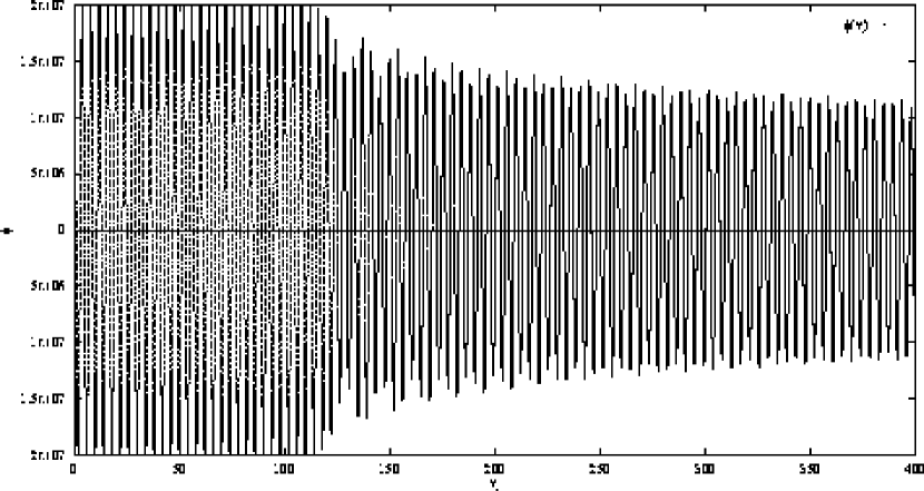
FIG. 1.: Plot of $\phi$ vs $\eta$, with $\text{$M_{\text{{P}}}$}/m=1.0\times 10^{14}$.

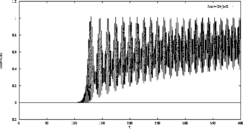
FIG. 2.: Plot of $\lambda\langle\text{$\varphi$}^{2}\rangle/2$ vs $\eta$, with $\text{$M_{\text{{P}}}$}/m=1.0\times 10^{14}$.

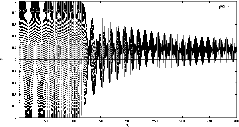
FIG. 3.: Plot of $\gamma$ vs $\eta$, with $\text{$M_{\text{{P}}}$}/m=1.0\times 10^{14}$.

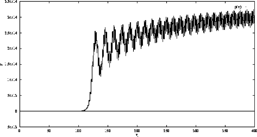
FIG. 4.: Plot of $\rho_{\text{{Q}}}$ vs $\eta$, with $\text{$M_{\text{{P}}}$}/m=1.0\times 10^{14}$.

FIG. 5.: Plot of $\phi$ vs $\eta$, with $\text{$M_{\text{{P}}}$}/m=1.0\times 10^{12}$.

FIG. 6.: Plot of $\lambda\langle\text{$\varphi$}^{2}\rangle/2$ vs $\eta$, with $\text{$M_{\text{{P}}}$}/m=1.0\times 10^{12}$.

FIG. 7.: Plot of $\gamma$ vs $\eta$, with $\text{$M_{\text{{P}}}$}/m=1.0\times 10^{12}$.

FIG. 8.: Plot of $\rho_{\text{{Q}}}$ vs $\eta$, with $\text{$M_{\text{{P}}}$}/m=1.0\times 10^{12}$.

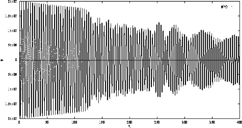
FIG. 9.: Plot of $\phi$ vs $\eta$, with $\text{$M_{\text{{P}}}$}/m=6.0\times 10^{10}$.

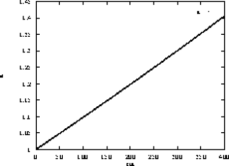
FIG. 10.: Plot of $a$ vs $\eta$, with $\text{$M_{\text{{P}}}$}/m=6.0\times 10^{10}$.

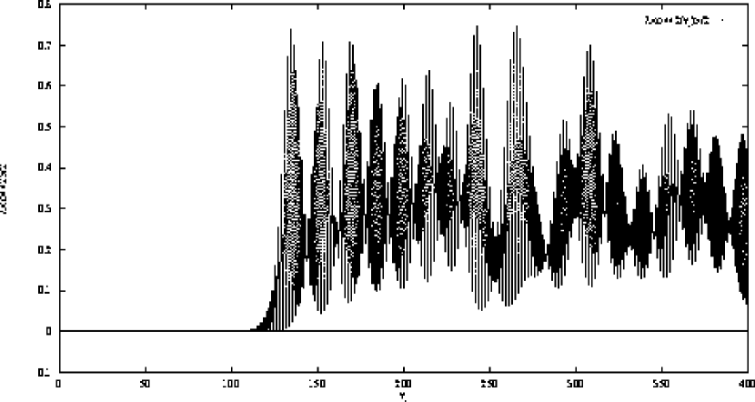
FIG. 11.: Plot of $\lambda\langle\text{$\varphi$}^{2}\rangle/2$ vs $\eta$, with $\text{$M_{\text{{P}}}$}/m=6.0\times 10^{10}$.

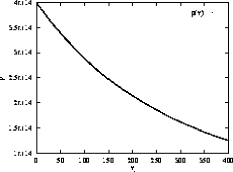
FIG. 12.: Plot of $\rho$ vs $\eta$, with $\text{$M_{\text{{P}}}$}/m=6.0\times 10^{10}$.

FIG. 13.: Plot of $\gamma$ vs $\eta$, with $\text{$M_{\text{{P}}}$}/m=6.0\times 10^{10}$.

FIG. 14.: Plot of $\rho_{\text{{Q}}}$ vs $\eta$, with $\text{$M_{\text{{P}}}$}/m=6.0\times 10^{10}$.

FIG. 15.: Plot of $\phi$ vs $\eta$, with $\text{$M_{\text{{P}}}$}/m=6.0\times 10^{9}$.

FIG. 16.: Plot of $a$ vs $\eta$, with $\text{$M_{\text{{P}}}$}/m=6.0\times 10^{9}$.

FIG. 17.: Plot of $\lambda\langle\text{$\varphi$}^{2}\rangle/2$ vs $\eta$, with $\text{$M_{\text{{P}}}$}/m=6.0\times 10^{9}$.

FIG. 18.: Plot of $\rho$ vs $\eta$, with $\text{$M_{\text{{P}}}$}/m=6.0\times 10^{9}$.

FIG. 19.: Plot of $\rho_{\text{{Q}}}$ vs $\eta$, with $\text{$M_{\text{{P}}}$}/m=6.0\times 10^{9}$.

REFERENCES

- [1] S. A. Ramsey and B. L. Hu, this issue, Phys. Rev. D 56, xxx (1997) [Report No. gr-qc/9706001].
- [2] A. H. Guth, Phys. Rev. D 23, 347 (1981).
- [3] K. Sato, Phys. Lett. B 99, 66 (1981).
- [4] A. Albrecht and P. J. Steinhardt, Phys. Rev. Lett. 48, 1220 (1982).
- [5] A. D. Linde, Phys. Lett. B 114, 431 (1982).
- [6] A. D. Linde, Phys. Lett. B 162, 281 (1985).
- [7] A. A. Starobinsky, in Field Theory, Quantum Gravity and Strings, Proceedings of the Seminar Series, Meudon and Paris, 1984–1985, edited by H. J. de Vega and N. Sánchez (Springer-Verlag, Berlin, 1986).
- [8] J. M. Bardeen and G. J. Bublik, Class. Quantum Grav. 4, 473 (1987).
- [9] R. H. Brandenberger, Rev. Mod. Phys. 57, 1 (1985), and references therein.
- [10] L. F. Abbott and S.-Y. Pi, Inflationary Cosmology (World Scientific, Singapore, 1986).
- [11] E. W. Kolb and M. S. Turner, in The Early Universe (Addison-Wesley, Redwood, CA, 1990), Chap. 8.
- [12] A. D. Linde, Particle Physics and Inflationary Cosmology (Harwood Academic, Chur, Switzerland, 1990).
- [13] A. D. Linde, “Prospects for Inflationary Cosmology,” 1996, Report No. astro-ph/9610077, (unpublished).
- [14] P. J. Steinhardt and M. S. Turner, Phys. Rev. D 29, 2162 (1984).
- [15] J. E. Lidsey et al., “Reconstructing the inflaton potential—an Overview,” 1995, Report No. astro-ph/9508078 (unpublished).
- [16] B. L. Hu, in Inner Space/Outer Space: The Interface Between Cosmology and Particle Physics, Fermilab, edited by E. W. Kolb et al. (University of Chicago Press, Chicago, 1986), pp. 479–488.
- [17] B. L. Hu, in Recent Developments in General Relativity: Proc. 4th Marcel Grossman Meeting, Rome, 1985, edited by R. Ruffini (North-Holland, Amsterdam, 1986).
- [18] N. D. Birrell and P. C. W. Davies, Quantum Fields in Curved Space (Cambridge University Press, Cambridge, United Kingdom, 1982), and references therein.
- [19] B. L. Hu, in Quantum Physics and the Universe, Proceedings of the Waseda Conference, edited by M. Namiki et al. (Pergamon Press, Tokyo, 1993), [Vistas Astron. 37, 391 (1993)].
- [20] B. L. Hu, in Proceedings of the Second Paris Cosmology Colloquium, Observatoire de Paris, June, 1994, edited by H. J. de Vega and N. Sánchez (World Scientific, Singapore, 1995), p. 111 [Report No. hep-th/9412052].
- [21] A. A. Starobinsky, Phys. Lett. B 91, 99 (1980).
- [22] B. L. Hu and D. J. O’Connor, Phys. Rev. D 34, 2535 (1986).
- [23] L. Parker, Phys. Rev. 183, 1057 (1969).
- [24] R. U. Sexl and H. K. Urbantke, Phys. Rev. 179, 1247 (1969).
- [25] Y. B. Zel’dovich, Zh. Eksp. Teor. Fiz. Pis. Red. 12, 443 (1970), [JETP Lett. 12, 307 (1971)].
- [26] Y. B. Zel’dovich and A. A. Starobinsky, Zh. Eksp. Teor. Fiz. 61, 2161 (1971), [Sov. Phys. JETP 34(6), 1159 (1972)].
- [27] B. L. Hu, Phys. Rev. D 9, 3263 (1974).
- [28] Y. B. Zel’dovich and A. A. Starobinsky, Zh. Eksp. Teor. Fiz. Pis. Red. 26, 323 (1977), [JETP Lett. 28, 252 (1977)].
- [29] B. L. Hu and L. Parker, Phys. Lett. A 63, 217 (1977).
- [30] B. L. Hu and L. Parker, Phys. Rev. D 17, 933 (1978).
- [31] F. V. Fischetti, J. B. Hartle, and B. L. Hu, Phys. Rev. D 20, 1757 (1979).
- [32] J. B. Hartle and B. L. Hu, Phys. Rev. D 20, 1772 (1979).
- [33] J. B. Hartle and B. L. Hu, Phys. Rev. D 21, 2756 (1980).
- [34] B. L. Hu, Phys. Lett. B 103, 331 (1981).
- [35] P. A. Anderson, Phys. Rev. D 29, 615 (1984).
- [36] D. J. O’Connor, B. L. Hu, and T. C. Shen, Phys. Lett. B 130, 31 (1983).
- [37] T. C. Shen, B. L. Hu, and D. J. O’Connor, Phys. Rev. D 31, 2401 (1985).
- [38] B. L. Hu and D. J. O’Connor, Phys. Rev. D 36, 1701 (1987).
- [39] A. L. Berkin, Phys. Rev. D 46, 1551 (1992).
- [40] B. L. Hu and D. J. O’Connor, Phys. Rev. Lett. 56, 1613 (1986).
- [41] E. Calzetta, B. L. Hu, and S. A. Ramsey, “Spinodal Decomposition via Correlation Dynamics of Quantum Fields” (in preparation).
- [42] B. L. Hu, Class. Quantum Grav. 10, S93 (1993).
- [43] A. H. Guth and S.-Y. Pi, Phys. Rev. D 32, 1899 (1985).
- [44] J. M. Cornwall and R. Bruinsma, Phys. Rev. D 38, 3146 (1988).
- [45] O. E. Buryak, Phys. Rev. D 53, 1763 (1996).
- [46] B. L. Hu, S. A. Ramsey, and A. Raval, “Nonequilibrium Inflaton Dynamics: Decoherence and Classical Stochastic Equations” (in preparation).
- [47] A. H. Guth and S.-Y. Pi, Phys. Rev. Lett. 49, 1110 (1982).
- [48] A. A. Starobinsky, Phys. Lett. B 117, 175 (1982).
- [49] S. W. Hawking, Phys. Lett. B 115, 295 (1982).
- [50] J. M. Bardeen, P. J. Steinhardt, and M. S. Turner, Phys. Rev. D 28, 679 (1983).
- [51] R. Brandenberger, R. Kahn, and W. H. Press, Phys. Rev. D 28, 1809 (1983).
- [52] V. F. Mukhanov, H. A. Feldman, and R. H. Brandenberger, Phys. Rep. 215, 203 (1992).
- [53] N. Deruelle, C. Gundlach, and D. Langlois, Phys. Rev. D 46, 5337 (1992).
- [54] B. L. Hu, J. P. Paz, and Y. Zhang, in The Origin of Structure in the Universe, edited by E. Gunzig and P. Nardone (Kluwer, Dordrecht, 1993), p. 227.
- [55] E. Calzetta and B. L. Hu, Phys. Rev. D 52, 6770 (1995).
- [56] A. Matacz, Phys. Rev. D 55, 1860 (1997).
- [57] B. L. Hu, in Proceedings of the Third International Workshop on Thermal Field Theory and Applications, Banff, Canada, 1993, edited by R. Kobes and G. Kunsatter (World Scientific, Singapore, 1994) [Report No. gr-qc/9403061].
- [58] J. Schwinger, J. Math. Phys. (N.Y.) 2, 407 (1961).
- [59] P. M. Bakshi and K. T. Mahanthappa, J. Math. Phys. (N.Y.) 4, 1 (1963); 4, 12 (1963).
- [60] L. V. Keldysh, Zh. Eksp. Teor. Fiz. 47, 1515 (1964) [Sov. Phys. JETP 20, 1018 (1965)].
- [61] A. Niemi and G. Semenoff, Ann. Phys. (N.Y.) 152, 105 (1981).
- [62] A. Niemi and G. Semenoff, Nucl. Phys. B230 [FS10], 181 (1984).
- [63] N. P. Landsman and C. G. van Weert, Phys. Rep. 145, 141 (1987).
- [64] G. Zhou, Z. Su, B. Hao, and L. Yu, Phys. Rep. 118, 1 (1985).
- [65] Z. Su, L. Y. Chen, X. Yu, and K. Chou, Phys. Rev. B 37, 9810 (1988).
- [66] B. S. DeWitt, in Quantum Concepts in Space and Time, edited by R. Penrose and C. J. Isham (Clarendon Press, Oxford, United Kingdom, 1986).
- [67] R. D. Jordan, Phys. Rev. D 33, 444 (1986).
- [68] E. Calzetta and B. L. Hu, Phys. Rev. D 35, 495 (1987).
- [69] E. Calzetta and B. L. Hu, Phys. Rev. D 37, 2878 (1988), and references therein.
- [70] E. Calzetta and B. L. Hu, Phys. Rev. D 40, 656 (1989).
- [71] R. P. Feynman and J. F. L. Vernon, Ann. Phys. (N.Y.) 24, 118 (1963).
- [72] R. P. Feynman and A. R. Hibbs, Quantum Mechanics and Path Integrals (McGraw-Hill, New York, 1965).
- [73] A. O. Caldeira and A. J. Leggett, Physica A 121, 587 (1983).
- [74] H. Grabert, P. Schramm, and G. L. Ingold, Phys. Rep. 168, 115 (1988).
- [75] B. L. Hu, J. P. Paz, and Y. Zhang, Phys. Rev. D 45, 2843 (1992).
- [76] B. L. Hu, J. P. Paz, and Y. Zhang, Phys. Rev. D 47, 1576 (1993).
- [77] E. Calzetta and B. L. Hu, Phys. Rev. D 49, 6636 (1994).
- [78] E. P. Wigner, Phys. Rev. 40, 749 (1932).
- [79] M. Hillery, R. F. O’Connell, M. O. Scully, and E. P. Wigner, Phys. Rep. 106, 121 (1984).
- [80] J. M. Cornwall, R. Jackiw, and E. Tomboulis, Phys. Rev. D 10, 2428 (1974).
- [81] E. Calzetta and B. L. Hu, in Directions in General Relativity, edited by B. L. Hu and T. A. Jacobson (Cambridge University Press, Cambridge, United Kingdom, 1993), Vol. 2 [Report No. gr-qc/9302013].
- [82] E. Calzetta and B. L. Hu, in Heat Kernel Techniques and Quantum Gravity, Vol. 4 of Discourses in Mathematics and Its Applications, edited by S. A. Fulling (Texas A&M University Press, College Station, TX, 1995) [Report No. hep-th/9501040].
- [83] E. Calzetta, S. Habib, and B. L. Hu, Phys. Rev. D 37, 2901 (1988).
- [84] E. Calzetta, Ann. Phys. (N.Y.) 190, 32 (1989).
- [85] S. A. Ramsey, B. L. Hu, and A. Stylianopoulos, “Nonequilibrium inflaton dynamics and reheating. II. Yukawa coupling and fermion production” (in preparation).
- [86] S. A. Ramsey and B. L. Hu, “Nonequilibrium inflaton dynamics and reheating. III. Fluctuations, dissipation, and entropy generation” (in preparation).
- [87] S. A. Ramsey and B. L. Hu, “Nonequilibrium inflaton dynamics and reheating. IV. Particle interaction and collisional thermalization” (in preparation).
- [88] E. W. Kolb, A. Linde, and A. Riotto, Phys. Rev. Lett. 77, 4290 (1996).
- [89] J. H. Traschen and R. H. Brandenberger, Phys. Rev. D 42, 2491 (1990).
- [90] L. A. Kofman, in Relativistic Astrophysics: A Conference in Honor of Igor Novikov’s 60th Birthday, edited by B. Jones and D. Markovic (Cambridge University Press, Cambridge, United Kingdom, 1996) [Report No. astro-ph/9605155].
- [91] L. F. Abbott, E. Farhi, and M. B. Wise, Phys. Lett. B 117, 29 (1982).
- [92] A. Albrecht, P. J. Steinhardt, M. S. Turner, and F. Wilczek, Phys. Rev. Lett. 48, 1437 (1982).
- [93] A. D. Dolgov and A. D. Linde, Phys. Lett. B 116, 329 (1982).
- [94] A. D. Dolgov and D. P. Kirilova, Yad. Fiz. 51, 273 (1990) [Sov. J. Nucl. Phys. 51 (1), 172 (1990)].
- [95] L. Kofman, A. Linde, and A. A. Starobinsky, Phys. Rev. Lett. 73, 3195 (1994).
- [96] Y. Shtanov, J. Traschen, and R. Brandenberger, Phys. Rev. D 51, 5438 (1995).
- [97] A. Dolgov and K. Freese, Phys. Rev. D 51, 2693 (1995).
- [98] R. Allahverdi and B. A. Campbell, Phys. Lett. B 395, 169 (1997).
- [99] L. Kofman, A. Linde, and A. A. Starobinsky, Phys. Rev. Lett. 76, 1011 (1996).
- [100] I. I. Tkachev, Phys. Lett. B 357, 35 (1996).
- [101] D. Boyanovsky, H. J. de Vega, R. Holman, and J. F. J. Salgado, Phys. Rev. D 54, 7570 (1996).
- [102] L. Parker and S. D. Fulling, Phys. Rev. D 9, 341 (1974).
- [103] S. A. Fulling, L. Parker, and B. L. Hu, Phys. Rev. D 10, 3905 (1974); 11, 1714(E) (1975).
- [104] S. A. Fulling and L. Parker, Ann. Phys. (N.Y.) 87, 176 (1974).
- [105] L. S. Brown and J. P. Cassidy, Phys. Rev. D 15, 2810 (1977).
- [106] J. Schwinger, Phys. Rev. 82, 664 (1951).
- [107] B. S. DeWitt, Dynamical Theory of Groups and Fields (Gordon and Breach, New York, 1965).
- [108] J. P. Paz, Phys. Rev. D 42, 529 (1990).
- [109] A. Stylianopoulos, Ph.D. thesis, University of Maryland, College Park, 1991.
- [110] D. Boyanovsky et al., Phys. Rev. D 51, 4419 (1995).
- [111] D. T. Son, Phys. Rev. D 54, 3745 (1996).
- [112] D. Boyanovsky et al., “Reheating the Post Inflationary Universe,” 1995, Report No. hep-ph/9505220 (unpublished).
- [113] D. Boyanovsky et al., in Proceedings of the School on String Gravity and Physics at the Planck Scale, Erice, Sicily, edited by N. Sánchez (World Scientific, Singapore, 1995) [Report No. hep-ph/9511361].
- [114] D. Boyanovsky et al., Phys. Rev. D 52, 6805 (1995).
- [115] J. Baacke, K. Heitmann, and C. Patzold, Phys. Rev. D (to be published).
- [116] D. I. Kaiser, Phys. Rev. D 53, 1776 (1996).
- [117] F. D. Mazzitelli, J. P. Paz, and C. El Hasi, Phys. Rev. D 40, 955 (1989).
- [118] S. Y. Khlebnikov and I. I. Tkachev, Phys. Lett. B 390, 80 (1997).
- [119] F. Cooper, S. Habib, Y. Kluger, E. Mottola, J. P. Paz, and P. Anderson, Phys. Rev. D 50, 2848 (1994).
- [120] F. Cooper, S. Habib, Y. Kluger, and E. Mottola, Phys. Rev. D 55, 6471 (1997).
- [121] D. Boyanovsky and H. J. de Vega, Phys. Rev. D 47, 2343 (1993).
- [122] D. Boyanovsky, H. J. de Vega, and R. Holman, Phys. Rev. D 49, 2769 (1994).
- [123] Y. Zhang, Ph.D. thesis, University of Maryland, College Park, 1991.
- [124] D. Boyanovsky, R. Holman, and S. P. Kumar, “Inflaton decay in de Sitter spacetime,” 1996, Report No. hep-ph/9606208 (unpublished).
- [125] G. F. Mazenko, Phys. Rev. D 34, 2223 (1986).
- [126] D. Boyanovsky et al., “Preheating in FRW Universes,” 1996, Report No. hep-ph/9609527 (unpublished).
- [127] A. D. Linde, Phys. Lett. B 129, 177 (1983).
- [128] A. D. Linde, “Lectures on Inflationary Cosmology,” 1994, Report No. hep-th/9410082 (unpublished).
- [129] D. Boyanovsky, D. Cormier, H. J. de Vega, and R. Holman, Phys. Rev. D 55, 373 (1997).
- [130] L. A. Kofman, “Comments on ‘Analytic and Numerical Study of Preheating Dynamics’,” 1996, Report No. hep-ph/9608341 (unpublished).
- [131] T. S. Bunch and P. C. W. Davies, Proc. R. Soc. London A 360, 117 (1978).
- [132] S. Y. Khlebnikov and I. I. Tkachev, Phys. Rev. Lett. 77, 219 (1996).
- [133] S. A. Fulling, Aspects of Quantum Field Theory in Curved Spacetime (Cambridge University Press, Cambridge, United Kingdom, 1989), Chap. 7.
- [134] C. W. Misner, K. S. Thorne, and J. A. Wheeler, Gravitation (Freemen, San Francisco, 1973).
- [135] B. S. DeWitt, Phys. Rep., Phys. Lett. 19C, 297 (1975).
- [136] S. Weinberg, Gravitation and Cosmology: Principles and Applications of the General Theory of Relativity (Wiley, New York, 1972).
- [137] G. F. Mazenko, W. G. Unruh, and R. M. Wald, Phys. Rev. D 31, 273 (1985).
- [138] I. S. Gradshteyn and I. M. Ryzhik, Tables of Integrals, Series, and Products (Academic Press, New York, 1964).
- [139] B. L. Hu and H. E. Kandrup, Phys. Rev. D 35, 1776 (1987).
- [140] P. Ramond, Field Theory: A Modern Primer (Addison-Wesley, Redwood, CA, 1990).
- [141] D. J. Toms, Phys. Rev. D 26, 2713 (1982).
- [142] F. D. Mazzitelli and J. P. Paz, Phys. Rev. D 39, 2234 (1989).
- [143] T. S. Bunch, J. Phys. A 13, 1297 (1980).
- [144] J. P. Paz and F. D. Mazzitelli, Phys. Rev. D 37, 2170 (1988).
- [145] R. G. Root, Phys. Rev. D 10, 3322 (1974).
- [146] B. L. Hu, Phys. Lett. A 71, 169 (1979).
- [147] P. A. Anderson, Phys. Rev. D 32, 1302 (1985).
- [148] W.-M. Suen, Phys. Rev. D 35, 1793 (1987).
- [149] W.-M. Suen and P. R. Anderson, Phys. Rev. D 35, 2940 (1987).
- [150] J. Z. Simon, Phys. Rev. D 41, 3720 (1990).
- [151] L. Parker and J. Z. Simon, Phys. Rev. D 47, 1339 (1993).
- [152] X. Jaén, J. Llosa, and A. Molina, Phys. Rev. D 34, 2302 (1986).
- [153] A. Ringwald, Ann. Phys. (N.Y.) 177, 129 (1987).