Abstract

We describe the physics potential of $e^{+}e^{-}$ linear colliders in this report. These machines are planned to operate in the first phase at a center–of–mass energy of 500 GeV, before being scaled up to about 1 TeV. In the second phase of the operation, a final energy of about 2 TeV is expected. The machines will allow us to perform precision tests of the heavy particles in the Standard Model, the top quark and the electroweak bosons. They are ideal facilities for exploring the properties of Higgs particles, in particular in the intermediate mass range. New vector bosons and novel matter particles in extended gauge theories can be searched for and studied thoroughly. The machines provide unique opportunities for the discovery of particles in supersymmetric extensions of the Standard Model, the spectrum of Higgs particles, the supersymmetric partners of the electroweak gauge and Higgs bosons, and of the matter particles. High precision analyses of their properties and interactions will allow for extrapolations to energy scales close to the Planck scale where gravity becomes significant. In alternative scenarios, like compositeness models, novel matter particles and interactions can be discovered and investigated in the energy range above the existing colliders up to the TeV scale. Whatever scenario is realized in Nature, the discovery potential of $e^{+}e^{-}$ linear colliders and the high–precision with which the properties of particles and their interactions can be analysed, define an exciting physics programme complementary to hadron machines.

1 Synopsis

High-energy $e^{+}e^{-}$ colliders have been essential instruments to search for the fundamental constituents of matter and their interactions. Merged with the experimental observations at hadron accelerators, a coherent picture of the structure of matter has evolved, that is adequately described by the Standard Model. The matter particles, leptons and quarks, can be classified in three families with identical symmetries. The electroweak and strong forces are described by gauge field theories, based on the symmetry group ${\rm SU}(3)_{C}\times{\rm SU}(2)_{L}\times{\rm U}(1)_{Y}$ [1, 2]. The third component of the Standard Model, still hypothetical, is the Higgs mechanism [3] through which the masses of the fundamental fermions and gauge bosons are generated.

The Standard Model has been tremendously successful in predicting the properties of new particles and the structure of the basic interactions. In many of its facets it has been tested at an accuracy significantly better than 1 percent. The Higgs mechanism however has not been established experimentally so far.

Despite the success in describing leptons, quarks and their interactions, the Standard Model cannot be considered as the ultima ratio of Nature. Neither the fundamental parameters, masses and couplings, nor the symmetry pattern are accounted for; these elements are merely built into the model. Moreover, gravity, with a nature quite different from the electroweak and strong forces, is not incorporated in the theory.

First steps which could lead us to solutions of these problems are associated with the unification of the electroweak and strong interactions [4], and with a possible supersymmetric extension of the model [5]. Supersymmetry provides a bridge from the presently explored energy scales to the scale of grand unified theories, which is close to the Planck scale where gravity becomes important. No such path is known, at the present time, for alternative compositeness scenarios which may include several new layers of matter between the low energy scale and the Planck scale.

Two strategies can be followed in future experiments to explore the area beyond the Standard Model and to reveal the signals of new physical phenomena. First, the properties of the particles and forces in the Standard Model may be affected by new energy scales. Precision studies of the top quark and the electroweak gauge bosons can thus reveal clues to the physics beyond the Standard Model. Second, if the machine energies are high enough to cross the relevant thresholds, new phenomena can be searched for directly and studied thoroughly. This is of course the prime raison d’$\hat{e}$tre for any new accelerator. While the presently operating collider facilities, the $e^{+}e^{-}$ collider LEP2, the $ep$ collider HERA and the $p\overline{p}$ collider Tevatron, cover the energy range up to a scale of 200 to 300 GeV, the $pp$ collider LHC and $e^{+}e^{-}$ linear colliders will enable us to explore the energy range up to the TeV scale.

On the basis of this dual approach, a variety of fundamental problems can be investigated that are so far unresolved within the Standard Model, and that demand experiments at energies beyond the range of the existing accelerators.

$(i)$ The mass of the top quark is much larger than the masses of all the other quarks and leptons, and even of the electroweak gauge bosons. Understanding the r$\hat{\rm o}$le of this particle in Nature is therefore a key element of future experiments. The experimental analysis of the $t\overline{t}$ threshold region in $e^{+}e^{-}$ collisions will allow the measurement of the top quark mass to an accuracy less than 200 MeV, improving the accuracy of about 2 GeV at the LHC significantly. This is a highly desirable goal since future theories of flavor dynamics should provide relations among the lepton masses, quark masses and mixing angles in which the heavy top quark is expected to play a key role. In addition, stringent tests of the electroweak sector in the Standard Model can be carried out at the quantum level when the top mass is known accurately. Analyses of the ($\gamma/Zt\bar{t}$) production vertices and of the $(tbW)$ decay vertex will determine the magnetic dipole moments of the top quark and the chirality of the decay current. Bounds on the ${\cal{CP}}$ violating electric dipole moments of the $t$ quark can be set in a similar way.

$(ii)$ The experimental study of the dynamics of the electroweak gauge bosons is an equally important task at high energy $e^{+}e^{-}$ colliders. The form and the strength of the triple and quartic couplings of these particles are uniquely prescribed by the non-abelian gauge symmetry of the Standard Model. The triple gauge boson couplings define the electroweak charges, the magnetic dipole moments and the electric quadrupole moments of the $W^{\pm}$ bosons. Any small deviation from the values of these parameters predicted in the Standard Model, will destroy the unitarity cancellations of the gauge theories. Their effect will therefore be magnified by increasing the energy, and the bounds will tighten considerably with rising energy.

$(iii)$ While the LHC can cover the canonical mass range, $e^{+}e^{-}$ colliders with an energy between 300 and 500 GeV are ideal instruments to search for Higgs particles throughout the mass range characterized by the scale of electroweak symmetry breaking. The mass of the Higgs particle is not determined by existing theory, but the intermediate mass range below $\sim 200$ GeV is theoretically a most attractive region for Higgs masses. In this scenario, Higgs particles remain weakly interacting up to the scale of grand unification, thus providing a path for the renormalization of the electroweak mixing angle $\sin^{2}\theta_{w}$ from the symmetry value 3/8 in grand unified theories down to $\sim 0.2$ which is close to the experimentally observed value 0.23. Once the Higgs particle is found, its properties can be studied thoroughly, i.e. the external quantum numbers ${\cal J}^{\cal{PC}}$ and the Higgs couplings, including the self-couplings of the particle. These are fundamental tests to establish the nature of the Higgs mechanism experimentally.

Even though many aspects of the Standard Model are experimentally supported to a very high accuracy, the embedding of the model into a more comprehensive theory is to be expected. The argument is based on the mechanism of the electroweak symmetry breaking. If the Higgs boson is light, the Standard Model can naturally be embedded in a grand unified theory. The large gap which exists between the low electroweak scale and the high grand unification scale in this scenario, can be stabilized by supersymmetry. If the Higgs boson is very heavy, or if no fundamental Higgs boson exists, new strong interactions between the massive electroweak gauge bosons are predicted by unitarity at the TeV scale. Thus, the next generation of accelerators which will operate in the TeV energy range, can uncover the structure of physics beyond the Standard Model.

The following two disgruent theories are the opposite endpoints in the arch of possible physics scenarios. They will be considered in detail:

$(i)$ The electroweak and strong forces are traced back to a common origin in Grand Unified Theories. This idea can be realized in various scenarios some of which predict new vector bosons and a plethora of new fermions. The mass scales of these novel particles could be as low as a few hundred GeV.

Intimately related to the grand unification of the gauge symmetries is Supersymmetry. This symmetry unifies matter and forces by pairing the associated fermionic and bosonic particles in multiplets. Several arguments strongly support the hypothesis that this symmetry is realized in Nature. (a) As argued before, supersymmetry stabilizes light masses of Higgs particles in the context of high energy scales as realized in grand unified theories. (b) The Higgs mechanism itself can be generated in supersymmetric theories as a quantum effect. The breaking of the electroweak gauge symmetry ${\rm SU}(2)_{L}\times{\rm U}(1)_{Y}$ can be induced radiatively while leaving the electromagnetic gauge symmetry ${\rm U}(1)_{EM}$ and the color gauge symmetry ${\rm SU}(3)_{C}$ unbroken for a top quark mass between 150 and 200 GeV. (c) This symmetry concept is strongly supported by the successful prediction of the electroweak mixing angle in the minimal version of the theory. The particle spectrum in this theory drives the evolution of the electroweak mixing angle from the GUT value 3/8 down to $\sin^{2}\theta_{w}$ = 0.2336 $\pm$ 0.0017; this prediction coincides with the experimentally measured value $\sin^{2}\theta_{w}^{exp}$ = 0.2315 $\pm$ 0.0003, within the theoretical uncertainty of less than 2 permille.

A spectrum of several neutral and charged Higgs bosons is predicted in supersymmetric theories. In nearly all scenarios, the mass of the lightest Higgs boson is less than $\sim 150$ GeV while the heavy Higgs particles have masses of the order of the electroweak symmetry breaking scale. Many other novel particles are predicted in supersymmetric theories. The scalar partners of the leptons could have masses in the range of $\sim 200$ GeV whereas squarks are expected to be considerably heavier. The lightest supersymmetric states are likely to be non-colored gaugino/higgsino states with masses possibly in the 100 GeV range. Searching for these supersymmetric particles will be one of the most important tasks at the LHC and at future $e^{+}e^{-}$ colliders. Moreover, the high accuracy which can be achieved in measurements of masses and couplings, will allow the reconstruction of the key elements of the underlying grand unified theories, which may be generated within the supersymmetric extension of gravity.

$(ii)$ In the alternative scenario of heavy or no fundamental Higgs bosons, strong interactions between electroweak bosons would be observed in the elastic scattering of these particles at TeV energies. New resonances would be formed, the properties of which would uncover the nature of the underlying microscopic interactions.

Not only would the properties and interactions of the electroweak bosons be affected but also those of the fundamental fermions, leptons and quarks in such a scenario. In the most dramatic departure from the Standard Model, these particles would be built up by new subconstituents corresponding to a new layer in the structure of matter. This alternative scenario would manifest itself in non-zero radii of quarks and leptons and the existence of novel bound states such as leptoquarks [6].

While new vector bosons and particles carrying color quantum numbers can be searched for very efficiently at the hadron collider LHC, $e^{+}e^{-}$ colliders provide in many ways unique opportunities to discover and explore the non-colored particles. This is most obvious in supersymmetric theories. Combining LEP2 analyses with future searches at the LHC, the individual light and heavy Higgs bosons can be found only in part of the supersymmetry parameter space; even if all channels are combined, the coverage of the entire parameter space is guaranteed only if non-supersymmetric decay modes of the Higgs bosons prevail. Squarks and gluinos can be searched for very efficiently at the LHC. Yet, the detailed experimental study of their properties is very difficult at this machine. Likewise, cascade decays proceeding in several steps, will allow the search for other, non-colored supersymmetric particles, yet a general model–independent analysis of gauginos/higgsinos and scalar sleptons can only be carried out at $e^{+}e^{-}$ colliders with well-defined kinematics at the level of the individual subprocesses. They will allow to perform high-precision studies which are impossible or very difficult to carry out at hadron colliders. Only the detailed knowledge of all the properties of the colored and non-colored supersymmetric states, gathered both at the LHC and $e^{+}e^{-}$ experiments, will finally enable us to reveal the structure of the underlying theory.

The physics programme of $e^{+}e^{-}$ linear colliders [?–?], summarized briefly in Table 1, is in many aspects complementary to the programme of the proton collider LHC. The properties of the top quark, the electroweak gauge bosons, the Higgs particles, the supersymmetric or other novel particles can be explored with high accuracy in a universal way, independent of favorable circumstances. These analyses will enable us to cover the energy range above the existing machines up to the TeV region in a conclusive form. This will provide essential information for elucidating the structure of matter at a much more basic level than accessible today – in particular, if grand unified theories are true, we will gain insight into the most fundamental levels of all.

THE ENERGY–PHYSICS MATRIX
  Top Gauge Bosons Higgs SUSY Compositeness   LC350 mass $W$ mass intermediate light Higgs/profile radii of   decays $\sin^{2}\theta_{w}$ Higgs/profile light $\tilde{\chi},\tilde{l}$ particles;   LC500 static elw. self-couplings intermediate light Higgs/profile excited   parameters new bosons/fermions Higgs/profile light $\tilde{\chi},\tilde{l}$ states;   LC1000 stat. param. self-couplgs. refined heavy Higgs/ heavy Higgs, $\tilde{\chi},\tilde{l}$ novel   refined new bosons/fermions profile light $\tilde{t},\tilde{b}$ particles:   LC2000 stat. param. new bosons/fermions heavy Higgs spectrum in toto: leptoquarks   refined strong $WW$ interact. Higgs potential $H,\tilde{\chi},\tilde{l},\tilde{q},\tilde{g}$ dileptons etc.

Table 1: The physics spectrum that can be explored in experiments at $e^{+}e^{-}$ linear colliders with energies extending from LEP up to 2 TeV.

The discussion in this report will focus on the physics with $e^{+}e^{-}$ colliders in the first phase, corresponding to center-of-mass energies above LEP2 up to $\sqrt{s}=500$ GeV; it will be assumed that the energy will be upgraded adiabatically up to about 800 GeV. Where necessary, we will refer to the second high-energy phase of the machine, anticipating an energy of about 1.6 TeV. To cover some physical scenarios it is necessary to extend the energy of the two phases up to 1 and 2 TeV, respectively. The integrated luminosity for energies at and below 500 GeV will in general be taken as $\int{\cal{L}}=$ 50 fb^-1, corresponding to operating the machine at these energies over 1 to 2 years. Above 500 GeV, the required integrated luminosity will be assumed to increase with the square of the c.m. energy. This implies about $\int{\cal{L}}$ = 125 fb^-1 at 800 GeV and 500 fb^-1 at 1.6 TeV.

The polarization of the electron and positron beams is a powerful tool in $e^{+}e^{-}$ colliders. At a technical level, the polarization of the beams can be used to enhance signals and to suppress backgrounds; quite often, polarized electron beams are sufficient for this purpose. At a deeper level, the polarization is of great advantage in performing the microscopic diagnosis of the properties of the fundamental particles, their interactions and the underlying symmetry concepts.

For some specific problems, operating linear colliders in the $e^{-}e^{-}$ and the $e\gamma$ or $\gamma\gamma$ satellite modes will be very useful. The high energy photons can be generated by Compton back-scattering of laser light on the high energy electron (and positron) bunches of the collider. The luminosities in these modes will be slightly reduced compared with the $e^{+}e^{-}$ collisions; in contrast to electron and positron bunches, electron–photon and photon–photon bunches do not attract each other while electron–electron bunches even repel each other. Longitudinal and transverse photon polarizations can be generated in Compton colliders by choosing the appropriate polarizations of the initial electron/positron and laser $\gamma$ beams.

The problems which can be tackled in the $e^{-}e^{-}$ [10] and the $\gamma$ [11] collider modes of the machine, will be addressed in the appropriate physics context. Initial states with exotic lepton quantum numbers are generated in $e^{-}e^{-}$ collisions, which are the proper basis for studies of dilepton states, doubly charged Higgs bosons and other particles, in particular Majorana neutrinos. $e\gamma$ and $\gamma\gamma$ collisions provide one of the most complex test grounds for QCD at high energies. Moreover, important aspects of Higgs physics and other areas in the electroweak sector can only be studied in $\gamma\gamma$ collisions.

In many examples the physics potential of $e^{+}e^{-}$ linear colliders will be compared with the results which are expected at the high-energy hadron-collider LHC. Any such comparison cannot be complete since only a selected set of processes has been simulated experimentally in detail so far. However, this set includes most of the problems associated with electroweak symmetry breaking and the Higgs mechanism, and essential elements of supersymmetry analyses at the LHC. The LHC comments are based primarily on the material presented in the ATLAS and CMS Technical Proposals [12], analyses of the DPF studies Ref.[13], and results presented at the LHCC Workshop on Supersymmetry [14].

2 Basic Standard Processes

The study of Standard Model processes at high energy colliders serves several purposes. On the one hand, high-precision analyses of these classical processes can be exploited to determine the properties of the particles in the Standard Model very accurately, and to detect or set limits on anomalous properties, such as anomalous multipole moments or potentially non-pointlike structures of the particles. On the other hand, Standard Model reactions are often unwanted background processes, which mask novel reactions predicted in the physical scenarios beyond the Standard Model and which should therefore be suppressed as much as possible.

Figure 1: (a) The basic processes of the Standard Model: $e^{+}e^{-}$ annihilation to pairs of fermions and gauge bosons. The cross sections are given for polar angles between $10^{0}<\theta<170^{0}$ in the final state. (b) Elastic/inelastic Compton scattering and $\gamma\gamma$ reactions. $\sqrt{s}$ is the invariant $e\gamma$ and $\gamma\gamma$ energy. The polar angle of the final state particles is restricted as in (a); in addition, the invariant $\mu^{+}\mu^{-}$ and $q\overline{q}$ masses in the inelastic Compton processes are restricted to $M_{inv}>50$ GeV.

a) Rates of the Basic Standard Processes

The theoretical basis of the standard processes is familiar from low-energy $e^{+}e^{-}$ collider experiments and will not be described in detail here.

The total cross sections are shown in Fig.1a for fermion pair production in $e^{+}e^{-}$ annihilation: $e^{+}e^{-}$ $\rightarrow f\bar{f}$. These processes are mediated by $s$–channel $\gamma$ and $Z$ exchanges, except for the Bhabha process which can also be generated by $t$–channel $\gamma$ and $Z$ exchanges. A cut in the polar angle of the observed electrons and positrons in the final state, $10^{0}<\theta<170^{0}$ corresponding to $|\cos\theta\mid<0.985$, has been introduced to remove the Rutherford pole; the size of the cut is slightly larger than the masks for the detector around the beam pipe. The magnitude of the cross sections, apart from the Bhabha process, varies typically between 0.5 and 8 pb at an energy of $\sqrt{s}$ = 500 GeV, corresponding to 2,500 to 15,000 events for an integrated luminosity of $\int{{\cal{L}}}=$ $50\mbox{ fb}^{-1}$. The cross section for Møller scattering follows closely the Bhabha cross section. [Program: CompHEP Ref.[15]].

The cross sections for $e^{+}e^{-}$ annihilation to pairs of gauge bosons, $e^{+}e^{-}$ $\rightarrow\gamma\gamma,Z\gamma,ZZ$ and $W^{+}W^{-}$, are presented in the same figure. Since the angular distributions peak strongly in the forward/backward directions, the same cut in the polar angle has been adopted as for Bhabha events. The size of the cross sections is similar to that for the fermionic annihilation cross sections.

The corresponding cross sections for initial state photons and mixed electron-photon states are collected in Fig.1b: $e\gamma\rightarrow e\gamma,eZ,ef\bar{f}$ and $\gamma\gamma\rightarrow WW,f\bar{f}$. [The cross sections of the $e\gamma$ and $\gamma\gamma$ processes are shown for the invariant $e\gamma$ and $\gamma\gamma$ energy $\sqrt{s}$; the results for the cross sections after folding with the Weizsäcker–Williams and Compton back-scattering spectra are discussed later.] The same polar-angle cut has been applied as before. Moreover, the difermion invariant masses in the inelastic Compton processes have been restricted to $M[f\bar{f}]>$ 50 GeV. Though still of similar overall size, the cross sections are in general slightly smaller than the annihilation cross sections for the cuts applied in the present analysis.

b) Polarization of Electron and Positron Beams

The polarization of the electron and positron beams gives a very effective means to control the effect of the Standard Model processes on the experimental analyses. By choosing the polarizations appropriately, different mechanisms which build up the Standard Model processes, can be switched on and off so that the rates of the various backgrounds can be studied and eventually much reduced. This is best-known for $W$ pair production in $e^{+}e^{-}$ annihilation, where the cross section for right-handed electrons is much smaller than the cross section for left-handed electrons.

Figure 2: The effect of beam polarization on the cross section for the production of $W^{+}W^{-}$ pairs. $U$ denotes unpolarized electron and positron beams, R:80 denotes 80% right-handedly polarized electron beams, and L:60 denotes 60% left-handedly polarized positron beams.

Beam polarization is also an indispensable tool for the identification and study of new particles and their interactions. In some cases, the event rates can be increased considerably by choosing the most suitable beam polarization for a specific reaction; for example, the cross section for Higgs production in $WW$ fusion increases by a factor 4 if the electron and positron beams are polarized. In others, the observation of polarization phenomena can add qualitatively new information on the basic properties of particles and interactions; a well-known example in this context is the analysis of mixed gaugino/higgsino and L/R sfermion states in supersymmetric theories.

In practice, the degree of polarization of electron beams is expected to be approximately 80%. Polarized positron beams are more difficult to generate, with a degree of polarization presumably in the range of 60% to 65%.

A few typical examples of Standard Model processes should illustrate the impact of beam polarizations on the analysis.

Fermion pair production $e^{+}e^{-}$ $\rightarrow f\bar{f}$. The dynamical impact of beam polarization on fermion-pair production through the annihilation channel is very modest. The polarization of the electron determines the polarization of the positron to be opposite in the annihilation process since gauge fields couple chirally flipped particles and antiparticles. Moreover, since the photon couplings are left/right symmetric, as well as the $Z$ couplings for electrons/positrons in the axial limit $\sin^{2}\theta_{w}\rightarrow 1/4$, the polarization does not have a dynamical impact on the total cross sections, but only the statistical weight affects the cross sections. If $\sigma_{p}$ is the annihilation cross section for both beams polarized, the cross section for polarized electrons/unpolarized positrons and for both beams unpolarized are both given approximately by $\frac{1}{2}\sigma_{p}$.

$W$ pair production $e^{+}e^{-}$ $\rightarrow W^{+}W^{-}$. This process is mediated by $t$–channel $\nu_{e}$ exchange, and $s$–channel $\gamma$ and $Z$ exchanges. A large fraction of the events is generated in the forward direction by the $t$–channel $\nu_{e}$-exchange mechanism. Choosing right-handedly polarized electrons, this mechanism is switched off. [Additional left-handed polarization of the positrons is statistically helpful but dynamically not required.] Moreover, the $s$–channel exchange diagrams are switched off at high energies for right-handedly polarized electrons; they do not couple to the $W^{3}$ component of the gauge fields in the intermediate state which is projected out by the charged $W$’s in the final state. The impact of the beam polarization on the differential cross section is demonstrated in Fig.2 where the cross sections for (partially) polarized beams are compared with the unpolarized cross section.

Single $W$ production. $W$ bosons are generated singly in the reactions $e^{+}e^{-}$ $\rightarrow e^{+}\nu_{e}W^{-}$ and $e^{+}e^{-}$ $\rightarrow\overline{\nu}_{e}e^{-}W^{+}$. These reactions are almost exclusively generated by Weizsäcker–Williams photons $e\to e\gamma$ and the subsequent processes $\gamma e^{-}\rightarrow W^{-}\nu_{e}$ and $e^{+}\gamma\rightarrow\overline{\nu}_{e}W^{+}$. The electron and positron beams both must be polarized in the right/left state to suppress this background reaction. This is one of the few cases where the suppression of a possible background requires the polarization of both beams.

c) Photon Beams

Intense high-energy photon beams can be generated by back-scattering of laser light off the incoming electrons and positron [16]. A large fraction of the energy can be transferred from the leptons to the photons in this configuration. The photon spectrum is rather broad however for unpolarized lepton and laser beams. The monochromaticity can be improved significantly if the incoming leptons and laser photons have opposite helicities, $P_{e}P_{\gamma}=-1$; the energy spectrum is given by:

$$P(y)=\frac{1}{1-y}+1-y-4r(1-r)-2P_{e}P_{\gamma}x_{0}r(2r-1)(2-y)$$ (1)

The fraction of energy transferred from the lepton to the final-state photon is denoted by $y$ and $r=y/[(1-y)x_{0}]$; the maximum value of $y$ follows from $y\leq x_{0}/(1+x_{0})$ with $x_{0}=4E\omega_{0}/m^{2}_{e}$. By tuning the frequency $\omega_{0}$ of the laser, the parameter $x_{0}$ must be chosen less than 4.83 to suppress kinematically the copious $e^{+}e^{-}$ pair production in the collision between the primary laser and the secondary high-energy photons.

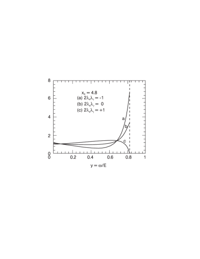
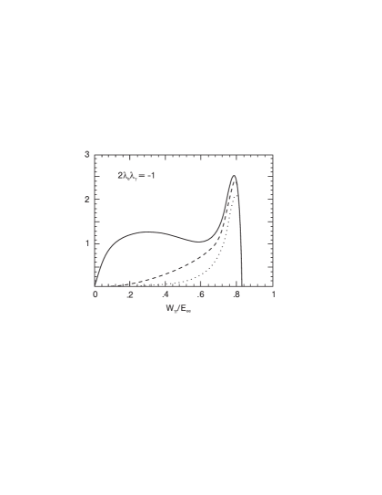
Figure 3: Left: The $\gamma$ energy spectrum in Compton back-scattering of laser light for three values of initial laser and electron beam helicities [17]. Right: The distribution of the $\gamma\gamma$ invariant mass in Compton back-scattering of laser light with opposite laser/electron helicities. The dashed curves demonstrate how the monochromaticity can be sharpened by separating the conversion from the collision point; c.f. Ref.[16].

The high-energy photon spectrum is shown for different helicities in Fig.3(left). The resulting $\gamma\gamma$ luminosity for the favorable case of opposite initial-state helicities [17] is shown in Fig.3(right). A clear, nearly mono-energetic maximum of the $\gamma\gamma$ luminosity is obtained, which is close to the maximum possible $\gamma\gamma$ invariant mass; the monochromaticity can be sharpened geometrically by choosing non-zero conversion distances from the $\gamma\gamma$ collision points.

High-energy $e\gamma$ and $\gamma\gamma$ collisions can be applied to investigate problems in many areas of particle physics. Outstanding examples are the production of Higgs bosons in $\gamma\gamma$ collisions to measure the $\gamma\gamma$ widths, the production of $W^{+}W^{-}$ pairs to determine the static magnetic and electric multipole moments of the $W$ bosons, and the photon structure functions and parton densities which provide deep insight into the structure of QCD. The cross sections for typical processes in the Standard Model are exemplified in Table 2 for two cases, with the $\gamma$ beams generated by Weizsäcker–Williams radiation and with the Compton $\gamma$ spectrum generated in unpolarized electron and laser beams.

	c.m. Energy	Cross Section $\sigma$[pb]			Cross Section $\sigma$[pb]
	$\sqrt{s_{ee}}$	$\gamma\gamma\rightarrow$			$e\gamma\rightarrow$
		$\mu^{+}\mu^{-}$	$u\bar{u}$	$W^{+}W^{-}$	$\nu_{e}W$	$eZ$	$e\mu^{+}\mu^{-}$	$eu\bar{u}$
WWR	500 GeV	2.4	1.4	0.2	2.9	0.3	0.1	0.2
	800 GeV	3.1	1.9	0.5	4.9	0.3	0.1	0.1
CBS	500 GeV	33	20	40	28	1.8	0.6	0.7
	800 GeV	17	10	49	32	0.9	0.3	0.3

Table 2: Cross sections of typical SM processes in $\gamma\gamma$ and $e\gamma$ collisions with the $\gamma$ beams generated by Weizsäcker–Williams radiation (WWR) and Compton back-scattering of laser light with the frequency parameter $x_{0}=4.83$ (CBS). The cross sections are given for polar angles of the visible particles between $10^{0}<\theta<170^{0}$ in the final state; in addition, the invariant $\mu^{+}\mu^{-}$ and $q\overline{q}$ masses are restricted to $M_{inv}>50$ GeV.

3 Top Quark Physics

Top quarks are the heaviest matter particles in the 3–family Standard Model. Introduced to incorporate ${\cal CP}$ violation [18], indirect evidence for the top quark had been accumulated quite early. After the isospin of the left-handed $b$ quarks was measured to be $I_{3}(b_{L})=-1/2$, derived from the $Z\rightarrow b\bar{b}$ width and the forward-backward asymmetry of $b$ jets in $e^{+}e^{-}$ annihilation, it was manifest that the symmetry pattern of the Standard Model required the existence of the top quark [19]. The top mass enters quadratically through radiative corrections [20] into the expression for the $\rho$ parameter, the relative strength between weak neutral and charged current processes. The high-precision measurements of the electroweak observables, in particular at the $e^{+}e^{-}$ colliders LEP1 and SLC, could be exploited to determine the top mass [21]: $m_{t}=173\,\pm\,23$ GeV. This prediction has recently been confirmed by the direct observation of top quarks at the Tevatron [22] with a mass of $m_{t}=174\,\pm\,6$ GeV, which is in striking agreement with the earlier electroweak analysis.

The large mass renders the top quark a very interesting object, the properties of which should be studied with high precision. Being the leading particle in the fermion spectrum of the Standard Model, it likely plays a key role in any theory of flavor dynamics. Moreover, due to the large mass, its properties are most strongly affected by Higgs particles and nearby new physics scales. High-precision measurements of the properties of top quarks are therefore mandatory at any future collider.

Since the lifetime of the $t$ quark is much shorter than the time scale $\Lambda^{-1}_{QCD}$ of the strong interactions, the impact of non-perturbative effects on the production and decay of top quarks can be neglected to a high level of accuracy [23]. The short lifetime provides a cut-off $k>\sqrt{2m_{t}\Gamma_{t}}$ for any soft non-perturbative and infrared perturbative interactions. The $t$ quark sector can therefore be analyzed within perturbative QCD. Unlike light quarks, the properties of $t$ quarks are reflected directly in the distributions of the decay jets and $W$ bosons, and they are not affected by the obscuring confinement and fragmentation effects.

$e^{+}e^{-}$ colliders are the most suitable instruments to study the properties of top quarks. Operating the machine at the $t\bar{t}$ threshold, the mass of the top quark can be determined with an accuracy that is an order of magnitude superior to measurements at hadron colliders. The static properties of top quarks, magnetic and electric dipole moments, can be measured very accurately in continuum top-pair production at high $e^{+}e^{-}$ colliders. Likewise, the chirality of the charged top-bottom current can be measured accurately in the decay of the top quark. In extensions of the Standard Model, supersymmetric extensions for example, top decays into novel particles, charged Higgs bosons and/or stop/sbottom particles, may be observed.

3.1 The Profile of the Top Quark: Decay

a) The Dominant SM Decay

With the top mass established as larger than the $W$ mass, the channel

$$t\rightarrow b+W^{+}$$

is the dominant decay mode, not only in the Standard Model but also in extended scenarios. The top quark width grows rapidly to $\sim 1.4$ GeV in the mass range $m_{t}\sim 175$ GeV [23]:

$$\Gamma(t\rightarrow b+W^{+})=\frac{G_{F}m^{3}_{t}}{8\sqrt{2}\pi}\left[1-\frac{m^{2}_{W}}{m^{2}_{t}}\right]^{2}\left[1+2\frac{m^{2}_{W}}{m^{2}_{t}}\right]$$ (2)

approximately given by $\Gamma_{t}\simeq 175\mbox{ MeV}\cdot[m_{t}/M_{W}]^{3}$. A large fraction, $p_{L}=m^{2}_{t}/(m^{2}_{t}+2m^{2}_{W})\approx 0.7$, of the decay $W$ bosons are longitudinally polarized. The rapid variation of $\Gamma_{t}$, proportional to the third power of $m_{t}$, is expected from the equivalence theorem of electroweak symmetry breaking in which the longitudinal $W$ component, dominating for large $t$ masses, can be identified with the charged Goldstone boson, the coupling of which grows with the $t$ mass. The width of the top quark is known to one-loop QCD and electroweak corrections [24]. The QCD corrections are about –10% for large top masses; the electroweak corrections turn out to be small, $\approx+2\%$ for a Higgs mass of $\sim$ 100 GeV.

The direct measurement of the top quark width is difficult. The most promising method appears to be provided by the analysis of the forward-backward asymmetry of $t$ quarks near the $e^{+}e^{-}$ production threshold. This asymmetry is generated by the overlap of parity-even $S$– and parity-odd $P$–wave production channels; it is therefore sensitive to the width $\Gamma_{t}$. Including the other threshold observables, cross section and momentum distributions, a precision of 10 to 20% can be expected for the measurement of $\Gamma_{t}$ in total [25].

Chirality of the $(tb)$ decay current. The precise determination of the weak isospin quantum numbers does not allow for large deviations of the $(tb)$ decay current from the left-handed prescription in the Standard Model. Nevertheless, since $V\!\!+\!\!A$ admixtures may grow with the masses of the quarks involved [$\sim\sqrt{m_{t}/M_{\ast}}$ through mixing with heavy mirror quarks of mass $M_{*}$, for instance], it is necessary to check the chirality of the decay current directly. The $l^{+}$ energy distribution in the semileptonic decay chain $t\rightarrow W^{+}\rightarrow l^{+}$ depends on the chirality of the current; for $V\!\!-\!\!A$ couplings it is given by $dN/dx_{l}\sim x^{2}_{l}(1-x_{l})$. Any deviation from the standard $V\!\!-\!\!A$ current would stiffen the spectrum, and it would lead to a non-zero value at the upper end-point of the energy distribution, in particular. A sensitivity of 5% to possible $V\!\!+\!\!A$ admixtures can be reached experimentally (see Ref.[26]). The sensitivity can be improved by analysing the decays of polarized top quarks which can be generated in collisions of longitudinally polarized electrons with un/polarized positrons.

b) Non–Standard Top Decays

Such decays could occur, for example, in supersymmetric extensions of the Standard Model: top decays into charged Higgs bosons and/or top decays to stop particles and neutralinos or sbottom particles and charginos:

$$t \rightarrow b+H^{+}\hskip 5.69054pt$$

$$t \rightarrow \tilde{t}+\tilde{\chi}^{0}_{1}\quad\mbox{and}\quad\tilde{b}+\tilde{\chi}^{+}_{1}$$

If kinematically allowed, branching ratios for these decay modes could be as large as 30%, given the present constraints on supersymmetric parameters, Fig.4 [27]. If LEP2 fails to discover supersymmetric particles, stop decays would become very unlikely while charged Higgs decays might still be frequent. The signatures for both decay modes are very clear and they are easy to detect experimentally [28]. Charged Higgs decays manifest themselves through chargino+neutralino decays, and $\tau$ decays with rates which are different from the universal $W$ decay rates in the Standard Model,

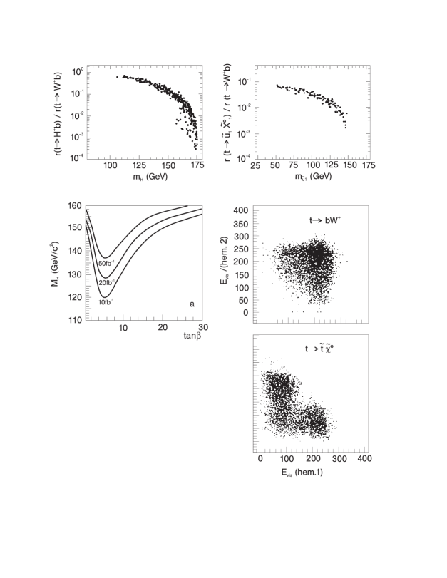
Figure 4: Left: Branching ratio of top decays to charged Higgs bosons, in supersymmetric theories. Shown is also the range of charged Higgs masses as a function of the coupling $\tan\beta$ that can be detected experimentally for a given luminosity of 10, 20, and 50 fb^-1. Refs.[27, 28]. Right: The decay of top quarks to stop particles and the lightest neutralino in supersymmetric theories. The lower plots present the energy distributions in the two event hemispheres for SM decays and SUSY decays which are characterized by missing energy due to escaping neutralinos. Refs.[27, 28].

thus breaking $\tau$ vs. $e,\mu$ universality. Final-state neutralinos, as the lightest supersymmetric particles, escape undetected in stop decays so that a large amount of missing energy would be observed in these decay modes.

Besides breaking the $V\!\!-\!\!A$ law for the chirality of the $t\rightarrow bW$ decay current, mixing of the top quark with other heavy quarks breaks the GIM mechanism if the new quark species do not belong to the standard doublet/singlet assignments of isospin multiplets. As a result, FCNC ($tc$) couplings of order $\sqrt{m_{t}m_{c}/M^{2}_{\ast}}$ can be induced. FCNC $t$ quark decays, for example $t\rightarrow c\gamma$ or $cZ$, may therefore occur at the level of a few permille; down to this level they can be detected experimentally [29]. The large number of top quarks produced at the LHC allows however to search for rare FCNC decays with clean signatures, such as $t\rightarrow cZ$, down to a branching ratio of less than $10^{-4}$.

3.2 Continuum Production: Static $t$ Parameters

The main production mechanism for top quarks in $e^{+}e^{-}$ collisions is the annihilation channel [30]

$$e^{+}e^{-}\stackrel{{\scriptstyle\gamma,Z}}{{\longrightarrow}}t\overline{t}$$

As shown in Fig.5, the cross section

$$\sigma(e^{+}e^{-}\rightarrow t\bar{t})=\beta{\textstyle\frac{3-\beta^{2}}{2}}\sigma^{VV}+\beta^{3}\sigma^{AA}$$ (3)

$$\sigma^{VV} = \frac{4\pi\alpha^{2}(s)}{s}e^{2}_{e}e^{2}_{t}+\frac{G_{F}\alpha(s)}{\sqrt{2}}e_{e}e_{t}v_{e}v_{t}\frac{m^{2}_{Z}}{s-m^{2}_{Z}}+\frac{G^{2}_{F}}{32\pi}(v^{2}_{e}+a^{2}_{e})v^{2}_{t}\frac{m^{4}_{Z}s}{(s-m^{2}_{Z})^{2}}$$

$$\sigma^{AA} = \frac{G^{2}_{F}}{32\pi}(v^{2}_{e}+a^{2}_{e})a^{2}_{t}\frac{m^{4}_{Z}s}{(s-m^{2}_{Z})^{2}}$$

[$v_{f},a_{f}$ being the $Z$ charges, and $\beta$ the velocity of the $t$ quarks] is of the order of 1 pb so that top quarks will be produced at large rates in a clean environment at $e^{+}e^{-}$ linear colliders, about 50,000 pairs for an integrated luminosity of $\int{{\cal{L}}}\sim$ $50\makebox{ fb}^{-1}$.

Figure 5: The cross section for the production of top-quark pairs in the continuum as a function of the total energy for three representative values of the top mass.

Since production and decay are not affected by the non-perturbative effects of hadronization, the helicities of the top quarks can be determined from the distribution of the jets and leptons in the decay chain $t\rightarrow b+W^{+}\rightarrow b+f\bar{f}^{\prime}$. The form factors of the top quark [31] in the electromagnetic and the weak neutral currents, the Pauli–Dirac form factors $F_{1}^{\gamma,Z}$ and $F_{2}^{\gamma,Z}$, the axial form factor $F_{A}^{Z}$ and the ${\cal{CP}}$ violating form factors $D_{A}^{\gamma,Z}$, can therefore be measured very accurately. The form factors $F_{1}^{\gamma,Z}$ and $F_{A}^{Z}$ are normalized to unity (modulo radiative corrections) and $F_{2}^{\gamma,Z}$ and $D_{A}^{\gamma,Z}$ vanish in the Standard Model. Anomalous values, in particular of the static magnetic- and electric-type dipole moments, could be a consequence of electroweak symmetry breaking in non-standard scenarios or of composite quark structures. Deviations from the values of the static parameters in the Standard Model have coefficients in the production cross section which grow with the c.m. energy.

Among the static parameters of the top quark which can be determined only at $e^{+}e^{-}$ linear colliders, the following examples are of particular interest:

$Z$ charges of the top quark. The form factors $F_{1}^{Z},F_{A}^{Z}$, or likewise the vectorial and axial $Z$ charges of the top quark, $v_{t}=+1-\frac{8}{3}\sin^{2}\theta_{w}$ and $a_{t}=+1$, can be determined from the $t\bar{t}$ production cross section [32]. Moreover, the production of top quarks near the threshold with longitudinally polarized beams leads to a sample of highly polarized quarks. The small admixture of transverse and normal polarization induced by $S$–wave/$P$–wave interference, is extremely sensitive to the axial $Z$ charge $a_{t}$ of the top quark [33].

Magnetic dipole moments of the top quark. If the electrons in the annihilation process $e^{+}e^{-}\rightarrow t\overline{t}$ are left-handedly polarized, the top quarks are produced preferentially as left-handed particles in the forward direction while only a small fraction is produced as right-handed particles in the backward direction [34]. As a result of this prediction in the Standard Model, the backward direction is most sensitive to small anomalous magnetic moments of the top quarks. The anomalous magnetic moments can be bounded to about 5 percent by measuring the angular dependence of the $t$ quark cross section.

Electric dipole moments of the top quark. Electric dipole moments are generated by ${\cal{CP}}$ non-invariant interactions. Non-zero values of these moments can be detected through non-vanishing expectation values of ${\cal{CP}}$–odd momentum tensors such as $T_{ij}\sim(q_{+}-q_{-})_{i}(q_{+}\times q_{-})_{j}$ or $A\sim p_{+}\cdot(q_{+}\times q_{-})$, with $p_{+},\,q_{\pm}$ being the unit momentum vectors of the initial $e^{+}$ and of the $W$–decay leptons, respectively. Sensitivity limits to $\gamma,Z$ electric dipole moments of $d^{\gamma,Z}_{t}<10^{-18}$ e cm can be reached [35] for an integrated luminosity of $\int{{\cal{L}}}=$ $20\mbox{ fb}^{-1}$ at $\sqrt{s}=500$ GeV if polarized beams are available.

3.3 Threshold Production: The Top Mass

Quark-antiquark production near the threshold in $e^{+}e^{-}$ collisions is, quite generally, of exceptional interest. For small quark masses, the long time which the particles remain close to each other, allows the strong interactions to build up rich structures of bound states and resonances. For the large top mass, the picture is different: The decay time of the states is shorter than the revolution time of the constituents so that toponium resonances can no longer form [23]. Traces of the $1S$ state give rise to a peak in the excitation curve which gradually levels off for quark masses beyond 150 GeV. Despite their transitory existence, the remnants of the toponium resonances nevertheless induce a fast rise of the cross section near the threshold. The steep rise provides the best basis for high-precision measurements of the top quark mass, superior to the reconstruction of the top mass in the decay final states at hadron colliders by more than an order of magnitude.

Since the rapid $t$ decay restricts the interaction region of the top quark to small distances, the excitation curve can be predicted in perturbative QCD [?–?]. The interquark potential is given essentially by the short distance Coulombic part,

$$V(R)\simeq-\frac{4}{3}\,\,\frac{\alpha_{s}(R)}{R}$$ (4)

modified by the confinement potential $\sim\sigma R$ at intermediate distances $R$ in the tail of the toponium resonances.

The excitation curve is built up primarily by the superposition of the $nS$ states. This sum can conveniently be performed by using non-relativistic Green’s function techniques:

$$\sigma(e^{+}e^{-}\rightarrow t\overline{t})_{thr}=\frac{24\pi^{2}\alpha^{2}e^{2}_{t}}{m^{4}_{t}}{\cal I}m\,G(\vec{x}=0;E+i\Gamma_{t})$$ (5)

The form and the height of the excitation curve are very sensitive to the mass of the top quark, but less to the value of the QCD coupling, Fig.6a. Since any increase of the $t$ quark mass can be compensated by a rise of the QCD coupling, which lowers the energy levels, the measurement errors of the two parameters are positively correlated.

Figure 6: Upper part: The cross section for the production of top quarks near the threshold. Demonstrated is the sensitivity of the cross section to the value of the top mass and the QCD coupling (normalized at the $Z$ mass). Lower part: The momentum spectrum of the top quarks near the threshold for a fixed total c.m. energy. The momentum depends strongly on the top mass, yet less on the QCD coupling. Refs.[37, 38].

This correlation can partially be resolved by measuring the momentum of the top quark [38] which is reflected in the momentum distribution of the decay $W$ boson. The $t$ momentum is determined by the Fourier transform of the wave functions of the overlapping resonances:

$$\frac{d\sigma}{dP_{t}}=\frac{24\pi^{2}\alpha^{2}e^{2}_{t}}{s}\frac{\Gamma_{t}}{m^{2}_{t}}|\hat{G}(P_{t},E+i\Gamma_{t})|^{2}$$ (6)

The top quarks, confined by the QCD potential, will have average momenta of order $\sim{\scriptstyle\frac{1}{2}}\alpha_{s}m_{t}$; together with the uncertainty $\sim\sqrt{\Gamma_{t}m_{t}}$ due to the finite lifetime, this leads to average momenta $<P_{t}>$ of about 15 GeV for $m_{t}\sim 175$ GeV. The measurement of the top mass and the QCD coupling by analysing the $t$ momentum spectrum is therefore independent of the analysis of the excitation curve, Fig.6.

The Higgs exchange between the top quarks generates a small attractive Yukawa force which enhances the attractive QCD force [39]. Since the range of the Yukawa force is of order $m^{-1}_{H}$, the effect on the excitation curve is small and restricted to Higgs mass values of order 100 GeV.

Detailed experimental simulations at $m_{t}\sim 175$ GeV predict the following sensitivity to the top mass and the QCD coupling, Fig.7, when the measurements of the excitation curve and the $t$ momentum spectrum are combined [29, 40]:

$$\delta m_{t} \approx 120\makebox{ MeV}$$

$$\delta\alpha_{s} \approx 0.003$$

These errors have been derived for an integrated luminosity of $\int{{\cal{L}}}$ $=50\makebox{ fb}^{-1}$.

At proton colliders a sensitivity of about 2 GeV has been predicted for the top mass, based on the reconstruction of top quarks from jet and lepton final states. Smearing effects due to soft stray gluons which are radiated off the $t$ quark before the decay and off the $b$ quark after the decay coherently, add to the complexity of the analysis. Thus, $e^{+}e^{-}$ colliders will improve our knowledge on the top-quark mass by at least an order of magnitude.

Why should it be desirable to measure the top mass with high precision? Two immediate reasons can be given:

$(i)$ Top and Higgs particles affect the relations between high-precision electroweak observables, $Z,W$–boson masses, electroweak mixing angle and Fermi coupling, through quantum fluctuations [41]. The radiative corrections can therefore be used to derive stringent constraints on the Higgs mass, $M_{H}=f(M_{Z},M_{W},m_{t})$, which must eventually be matched by the direct measurement of the Higgs mass at the LHC and the linear collider. Assuming a measurement of the $W$ mass with an accuracy of 15 MeV [see

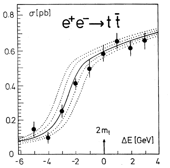
Figure 7: Excitation curve of the top quarks including initial-state radiation and beamstrahlung. The errors of the data points correspond to an integrated luminosity of $\int{\cal{L}}$ = 50 fb^-1 in toto. The dotted curves indicate shifts of the top mass by 200 and 400 MeV. Ref.[29, 40].

later], tight constraints on the Higgs mass can be derived if the top mass is measured with high accuracy. This is demonstrated in Fig.8, where the error on the predicted Higgs mass in the Standard Model is compared for two different errors on the top mass, $\delta m_{t}=4$ GeV and 200 MeV. The error in $\alpha(M_{Z}^{2})$ has been assumed at the ultimate level of $3\cdot 10^{-4}$ [42]. [Doubling this error to the present standard value does not have a dramatic effect.] It turns out that the Higgs mass can finally be extracted from the high-precision electroweak observables to an accuracy of about 17%. Thus, high precision measurements of the top mass allow the most stringent tests of the mechanism breaking the electroweak symmetries at the quantum level.

$(ii)$ Fermion masses and mixing angles are not linked to each other within the general frame of the Standard Model. This deficiency will be removed when in a future theory of flavor dynamics, which may be based for example on superstring theories, these fundamental parameters are interrelated. The top quark, endowed with the heaviest mass in the fermion sector, will very likely play a key rôle in this context. In the same way as present measurements test the relations between the masses of the electroweak $W,Z$ vector bosons in the Standard Model, similar relations between lepton and quark masses will have to be scrutinized in the future. With a relative error of about 1 permille, the top mass will be the best-known mass value in the quark sector, the only value matching the precision of the $\tau$ mass in the lepton sector.

Figure 8: The error on the Higgs mass extracted from the radiative corrections to the high-precision electroweak observables: $M_{H}=\rho(M_{Z},M_{W},m_{t})$. The input values [$\delta M_{W},\delta m_{t}$] are assumed as follows: LEP2 + Tevatron = [30 MeV, 4 GeV]; LHC/Tev33 = [15 MeV, 2 GeV], and LC = [15 MeV, 200 MeV]. The LHC lines fall in between the dashed and thin solid lines.

4 QCD Physics

4.1 Annihilation Events

The annihilation of $e^{+}e^{-}$ into hadrons provides a high-energy source of clean quark and gluon jets: $e^{+}e^{-}\to\gamma^{*}/Z^{*}\to q\overline{q},\ q\overline{q}g$ … This has offered unrivaled opportunities for QCD tests at machines such as PETRA and LEP. The program will be continued at a linear collider, although separation from new ‘backgrounds’ such as top and $W/Z$ pair production will require more delicate analyses of multijet events. Conversely, the study of these other processes, as well as the new particle searches, require a good understanding of the annihilation events. Topics of interest for QCD per se include the study of multijet topologies, the energy increase of charged multiplicity, particle momentum spectra and their scaling violations, angular ordering effects, hadronization phenomenology (power corrections), and so on.

One of the key elements of quantum chromodynamics is asymptotic freedom [43], a consequence of the non-abelian nature of the color gauge symmetry. This fundamental aspect has been tested in many observables measured at $e^{+}e^{-}$ colliders and other accelerators between a minimum $Q^{2}$ of order 4 GeV² up to $4\cdot 10^{4}\makebox{ GeV}^{2}$, ranging from the $\tau$ lifetime to multi-jet distributions in $Z$ decays. The range of $Q^{2}$ can be extended at $e^{+}e^{-}$ linear colliders by as much as two orders of magnitude to a value $Q^{2}\sim 4\cdot 10^{6}\makebox{ GeV}^{2}$, Fig. 9. The most sensitive observable in this energy range is the fraction of events with 2, 3, 4, … jets in the final state of $e^{+}e^{-}\rightarrow$ hadrons [44]. The results of the simulations can be nicely illustrated, Fig. 9, by presenting the evolution of the three-jet fraction in the variable $1/\log Q^{2}$. Asymptotic freedom predicts this dependence to be linear, modified only slightly by higher order corrections. Based on the present theoretical accuracy of the perturbative jet calculations, the error with which the QCD coupling at $\sqrt{s}=500$ GeV can be measured, is expected to be $\delta\alpha_{s}(M_{Z}^{2})\simeq 0.005$ matching the error which can be expected from the analysis of the top excitation curve at threshold. If the theoretical analysis of the jet rates can be improved, the error on $\alpha_{s}$ can be reduced significantly.

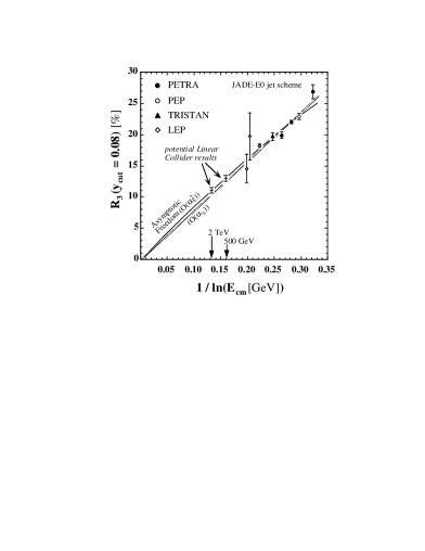
Figure 9: Left: The energy dependence of the three-jet fraction in annihilation events. Right: The energy dependence of $\alpha_{s}$. [Current data and simulated LC points; Ref.[44]]

4.2 $\gamma\gamma$ Events

$\gamma\gamma$ interactions provide a complementary way to study many aspects of new physics. These applications are covered in the respective physics sections. In addition, the objective of a $\gamma\gamma$ physics program is to bring our understanding of the photon to the same level as HERA is achieving for the proton. Since the photon is the more complex of the two, as described below, this will offer new insights in QCD [11, 45].

Linear $e^{+}e^{-}$ colliders offer three sources of photons: $(i)$ bremsstrahlung [46], $(ii)$ beamstrahlung [47] and $(iii)$ potentially, from laser backscattering [16]. The bremsstrahlung source provides a spectrum of different photon energies and virtualities, but distributions are peaked at the lower end so that the more interesting studies at higher $\gamma\gamma$ energies are limited by statistics. Since beamstrahlung is a drawback for the normal $e^{+}e^{-}$ physics program, current machine designs attempt to reduce the beamstrahlung energy to a minimum, so that it may not be interesting for $\gamma\gamma$ physics. The laser backscattering option, on the other hand, offers the prospect of intense beams of real photons with an energy up to about 80% of the $e^{\pm}$ beam. With one or both beams backscattered it would be possible to study both deep inelastic scattering off a real photon and the interactions of two real photons at very high energies. The $\gamma\gamma$ studies are possible for both the $e^{+}e^{-}$ and the $e^{-}e^{-}$ modes; the latter would have some advantages in terms of lower backgrounds from other processes.

(a) The nature of the photon is complex. A photon can fluctuate into a virtual $q\overline{q}$ pair. The low-end part of the spectrum of virtualities is in a non-perturbative régime, where the Vector Meson Dominance (VMD) model can be used to approximate the photon properties by those of mesons with the same quantum numbers as the photon — mainly the $\rho^{0}$. The high-end part, on the other hand, is perturbatively calculable [48]. These ‘resolved’ parts of the photon with a spectrum of order $\alpha/\alpha_{s}$, can undergo strong interactions of order $\alpha_{s}$. Therefore they can dominate in cross section over the nonfluctuating ‘direct’ photons, whose interactions are of ${\cal O}(\alpha)$. The direct/resolved subdivision of interactions is unambiguous only to leading order, but also in higher orders it is possible to introduce a pragmatic subdivision, as has been demonstrated for $\gamma p$ physics at HERA. In the direct interactions the full photon energy is used to produce (high-$p_{\perp}$) jets, whereas the resolved photon leaves behind a beam remnant that does not participate in the primary interaction.

(b) The total cross section of $\gamma\gamma$ interactions is not understood from first principles. This situation is analogous with that for $pp/p\overline{p}$ and $\gamma p$ cross sections, but not identical. Therefore the possibility of systematic comparisons between $pp/p\overline{p}$, $\gamma p$ and $\gamma\gamma$ at a wide range of energies could shed light on the mechanisms at play [49].

Figure 10: The inelastic $\gamma\gamma$ cross section, i.e. the major part of the total $\gamma\gamma$ cross section, as a function of the $\gamma\gamma$ c.m. energy $\sqrt{s}$; Ref.[50].

The uncertainty in our current understanding is illustrated in Fig. 10, where three representative models are compared with low-energy data [50]. The Pomeron/SaS model is based on a simple ansatz with an $s^{0.08}$ asymptotic rise, in accord with $pp/p\overline{p}$ and $\gamma p$ experience. The minijet model is based on an eikonalization of the mini-jet cross section, with parameters extrapolated from the $\gamma p$ case. In the ‘dual topological unitarization’ model of Phojet also elastic and diffractive topologies are included in an eikonalization approach. It is worth noticing that all three predictions, as well as current LEP data, are consistent with a straightforward application of factorization and Regge behavior. The long-dashed region in the figure is obtained from the ansätze

$$\sigma_{ab}^{tot}=X_{ab}s^{\epsilon}+Y_{ab}s^{-\eta}$$ (7)

with $\epsilon=0.079$ and $\eta=0.46$ from the average for all high energy cross-sections, X and Y extracted from pp and $\gamma p$ data, according to $X_{\gamma\gamma}=X_{\gamma p}^{2}/X_{pp}$. The band corresponds to the error induced by the uncertainty on $X_{\gamma p}$.

The total cross section can be subdivided into several components. The elastic and diffractive ones correspond to events like $\gamma\gamma\to\rho^{0}\rho^{0}$, $\gamma\gamma\to\rho^{0}X$ and $\gamma\gamma\to X_{1}X_{2}$. Studies of these would further probe the nature of the photon and the Pomeron, while $\gamma\gamma\to\pi^{0}X$ and $\gamma\gamma\to\pi^{0}a_{2}^{0}$ would probe the Odderon [51]. A study of the $p_{\perp}$ dependence could highlight the transition from the soft Pomeron to the perturbative one. Studies of rapidity gap physics could provide further insights into an area that currently is attracting intense interest at HERA. However, it will be difficult to realize the full potential of many of these topics, since most of these particles are produced at very small angles below 40 mrad, where they will be undetectable.

(c) The cross section for deep inelastic scattering off a real photon, $e\gamma\to e^{\prime}X$, is expressed in terms of the structure functions of the photon [48]. To leading order, these are given by the quark content, e.g.

$$F_{2}^{\gamma}(x,Q^{2})=\sum_{q}e_{q}^{2}\left[xq^{\gamma}(x,Q^{2})+x\overline{q}^{\gamma}(x,Q^{2})\right]~{}.$$ (8)

The parton distributions obey $Q^{2}$ evolution equations which, in addition to the homogeneous terms familiar for the proton, also include inhomogeneous terms related to the $\gamma\to q\overline{q}$ branchings. Experimental input is needed to specify the initial conditions at some reference scale $Q_{0}^{2}$. Data at larger $Q^{2}$ and smaller $x$ values than currently accessible would both provide information on the quark/gluon structure of the photon and offer consistency checks of QCD.

(a)

(b)

Figure 11: (a) Simulated data points for $e$ tagging outside 175 mrad for 10 fb^-1 at 500 GeV, compared with LEP2 expectations; Ref.[52]. (b) Simulated data points if tagging is feasible outside 40 mrad.

Electron tagging outside of a cone of about 175 mrad will give access to a previously unexplored high-$Q^{2}$ range, Fig. 11a [52], but will give neither overlap with LEP 2 results nor sensitivity to the small-$x$ region. To achieve the overlap with LEP 2, one needs an electron tagging device inside the shielding, down to about 40 mrad, Fig. 11b. This is however still not sufficient to unfold $x$ measurements in the region $x\leq 0.1$, since small $x=Q^{2}/(Q^{2}+W^{2})$ correspond to large $W^{2}$, where an unknown part of the hadronic system disappears undetected in the forward direction. In order to circumvent this problem, and also for reducing the main systematic errors at high $x$, the $e\gamma$ laser backscattering mode is ideal.

Figure 12: Left: Parton-level jet cross sections for interactions with transverse momenta above 5 GeV and 20 GeV, respectively, as a function of the $\gamma\gamma$ c.m. energy. Each interaction gives two jets. The total $\gamma\gamma$ cross section is shown for comparison. Right: Next-to-leading order calculations of the jet $p_{\perp}$ spectrum [54] at 500 GeV. The $\gamma\gamma$ cross section has been convoluted with the photon flux from bremsstrahlung and beamstrahlung. The spectrum is also shown subdivided into three components: direct (DD), once-resolved (DR) and twice-resolved (RR).

The longitudinal structure function $F_{L}$ of the photon, though very interesting theoretically since it is scale-invariant in leading order [53] in contrast to $F_{2}^{\gamma}$, appears to be very difficult to measure, having a coefficient $y^{2}$ in the cross section, the square of the scaled energy transfer which is generally small.

(d) A non-negligible fraction of the total $\gamma\gamma$ cross section involves the production of jets, Fig. 12(left). The jet events [55] may be classified according to whether the two photons are direct or one or both are resolved. The full photon energy is available for jet production in direct processes, so this event class dominates at large $p_{\perp}$ values, Fig. 12(right). Here our understanding of the photon can be tested essentially parameter-free. At lower $p_{\perp}$ values the resolved processes take over, since the evolution equations build up large gluon densities at small $x$ and since the gluon-exchange graphs that dominate here are more singular in the $p_{\perp}\to 0$ limit. The low-$p_{\perp}$ region therefore is interesting for constraining the parton densities of the photon. It complements the quark-dominated information obtained from $F_{2}^{\gamma}(x,Q^{2})$. The standard analysis strategy is based on jet reconstruction, but alternatively the inclusive hadron production as a function of $p_{\perp}$ could be used [56]. These processes are powerful instruments to constrain the gluon density of the resolved photon.

Figure 13: Left: The cross section for charm production as a function of $e^{+}e^{-}$ energy, total and subdivided; Ref.[57]. Right: The hadronic (dashed line) and the pointlike component (solid lines) of $F_{2}^{\gamma,c\overline{c}}/\alpha$ at $Q^{2}=200$ GeV². The two sets of curves correspond to leading and next-to-leading order calculations; in the small–$x$ range: dashed, upper curve: LO, lower curve: NLO; solid, upper curve: NLO, lower curve: LO. Ref.[59].

(e) The photon couplings favor charm production; in the direct channel $\gamma\gamma\to q\overline{q}$ the charge factor is $e_{q}^{4}$. Therefore significant charm rates can be expected, Fig. 13a. At 500 GeV the once-resolved processes dominate, and thereby the parton content of the photon is probed. $J/\Psi$ production is dominated by the process $\gamma+g\rightarrow J/\Psi+g$, and thus probes the gluon content of the photon specifically [58]. A related test is offered by the charm component of $F_{2}^{\gamma}(x,Q^{2})$, Fig. 13b, [59]. The pointlike part $\gamma^{*}\gamma\to c\overline{c}$ is perturbatively calculable, while the hadronic one is dominated by $\gamma^{*}g\to c\overline{c}$ and thus probes the gluon content of the photon.

(f) Double-tagged $\gamma^{*}\gamma^{*}$ events occur at low rates. Compared with the Born-term cross section for $\gamma^{*}\gamma^{*}\to q\overline{q}$, the evolution of a BFKL-style small-$x$ parton distribution inside the photon would boost event rates by more than a factor 10. In fact, this process may be considered the ultimate test of BFKL dynamics [60]. With tagging down to 30–40 mrad it will be possible to detect such a phenomenon, if present, but more detailed studies would be limited by the low statistics [61].

5 Electroweak Gauge Bosons

5.1 $W,Z$ Bosons in the Standard Model

The fundamental electroweak and strong forces appear to be of gauge theoretical origin. This is one of the outstanding theoretical and experimental results in the past three decades. While the non-abelian symmetry of QCD, manifest in the self-coupling of the gluons, has been successfully demonstrated in the distribution of hadronic jets in $Z$ decays, only indirect evidence has been accumulated so far for the electroweak $W^{\pm},Z,\gamma$ sector, based on loop corrections to electroweak low-energy parameters and $Z$ observables. The direct evidence from recent Tevatron and LEP2 analyses is still feeble. Deviations from the prescriptions of gauge symmetry manifest themselves in the cross sections with coefficients $(\beta\gamma)^{2}$, destroying fine-tuned unitarity cancellations [62] at high energies. Since the deviations of the static parameters from the SM values are expected to be of order $[M_{W}/\Lambda]^{j}$, $\Lambda$ denoting the energy scale at which the Standard Model breaks down, only the very high energies at the LHC and $e^{+}e^{-}$ linear colliders will allow stringent direct tests of the self-couplings of the electroweak gauge bosons.

The gauge symmetries of the Standard Model determine the form and the strength of the self-interactions of the electroweak bosons: the triple couplings $WW\gamma,WWZ$ and the quartic couplings. Deviations from the form and the strength of these vertices predicted by the gauge symmetry, as well as novel couplings like $ZZZ$ and $ZZZZ$ in addition to the canonical SM couplings, could however be expected in more general scenarios, in models with composite $W,Z$ bosons, for instance. Other examples are provided by models in which the $W,Z$ bosons are generated dynamically or interact strongly with each other.

Pair production of $W$ bosons in $e^{+}e^{-}$ collisions,

$$e^{+}e^{-}\longrightarrow W^{+}W^{-}$$

is the best-suited process to study the electroweak gauge symmetries. The high efficiency for reconstructing $W,Z$ bosons from hadronic and leptonic decays in the clean environment of $e^{+}e^{-}$ collisions makes a 500 GeV collider superior to the LHC. Deviations from the predictions of the Standard Model for the total cross section [63], c.f. Fig.14,

Figure 14: The cross section for $W^{+}W^{-}$ pair production, broken down to the transverse and longitudinal helicity components of the $W$ bosons.

$$\sigma(e^{+}e^{-}\rightarrow W^{+}W^{-}) = \frac{\pi\alpha^{2}(s)}{2s_{w}^{4}}\frac{\beta}{s}\left\{\left[1+\frac{2M_{W}^{2}}{s}+\frac{2M_{W}^{4}}{s^{2}}\right]\frac{1}{\beta}\log\frac{1+\beta}{1-\beta}-\frac{5}{4}\right.$$ (9)

$$+\frac{M_{Z}^{2}(1-2s_{w}^{2})}{s-M_{Z}^{2}}\left[2\left(\frac{M_{W}^{4}}{s^{2}}+\frac{2M_{W}^{2}}{s}\right)\frac{1}{\beta}\log\frac{1+\beta}{1-\beta}-\frac{s}{12M_{W}^{2}}-\frac{5}{3}-\frac{M_{W}^{2}}{s}\right]$$

$$\left.+\frac{M_{Z}^{4}(8s_{w}^{4}-4s_{w}^{2}+1)\beta^{2}}{48(s-M_{Z}^{2})^{2}}\left[\frac{s^{2}}{M_{W}^{4}}+\frac{20s}{M_{W}^{2}}+12\right]\right\}$$

[$s_{w}^{2}=\sin^{2}{\theta_{w}}$ and $\beta$ denoting the $W$ velocity] would signal non-standard self-couplings of the electroweak gauge bosons. The most stringent limits can be derived from the angular distributions of the $W$ pairs and their helicities [64] (derived from the decay angular distributions). These analyses can be carried out at collider energies of 500 GeV, promising sensitivities to non-standard couplings of order 1 percent and better.

If light Higgs bosons do not exist, the electroweak $W$ bosons become strongly interacting particles at high energies to comply with the requirements of quantum-mechanical unitarity. Strong interactions between $W$ bosons can be studied in (quasi) elastic $WW\rightarrow WW$ scattering [65, 66] and in $WW$ pair production [67, 68] at energies in the TeV range.

a) High Precision Measurements of $W$–Mass and $\sin^{2}\theta_{w}$

The mass of the $Z$ boson has been measured in $e^{+}e^{-}$ collisions at LEP1 to an accuracy of 2 MeV. To obtain a similar precision on the $W$ mass is therefore a natural goal of future experiments. Several methods can be used to measure the W mass at $e^{+}e^{-}$ linear colliders. Since these machines can be operated near the WW threshold with high luminosity, one of the promising methods [69] is the scan of the threshold region near $\sqrt{s}=161$ GeV where the sensitivity of the cross section to the W mass is maximal. [This scan will eventually allow to measure also the W width]. Since the uncertainty on the beam energy is expected to be reduced, using high-precision analyses of $Z\gamma$ and $ZZ$ events, to well below 10 MeV and the uncertainty in the measurement of the cross section to well below one percent, an accuracy

$$\delta M_{W}\approx 15{\rm MeV}$$

should finally be reached for the W mass.

The same accuracy will also be achieved by reconstructing the $W$ bosons in mixed lepton/jet $WW$ final states. With an experimental resolution of 3 to 4 GeV on an event-by-event basis, the final error on the $W$ mass can be expected below $\delta M_{W}\sim 15$ MeV for an integrated luminosity of 50 to 100 fb^-1 at energies $\sqrt{s}$ of 350 and 500 GeV [70]. This measurement of the $W$ mass can be performed in parallel to other experimental analyses so that the luminosity requirement for this standard channel remains within the anticipated frame.

A corresponding high-precision measurement of the electroweak mixing angle $\sin^{2}\theta_{w}$ can be performed by operating the collider at the $Z$ mass where about $10^{7}$ $Z$ bosons can be expected in two months of running. The most sensitive observable for measuring $\sin^{2}\theta_{w}$ is the left/right asymmetry for polarized electron/positron beams,

$$A_{LR}=\frac{2v_{e}a_{e}}{v_{e}^{2}+a_{e}^{2}}$$ (10)

where $v_{e}=-1+4\sin^{2}\theta_{w}$ and $a_{e}=-1$ are the vectorial and axial $Z$ charges of the electron, respectively. For $\sin^{2}\theta_{w}$ close to 1/4, the sensitivity is enhanced by nearly a full order of magnitude, $\delta\sin^{2}\theta_{w}\approx\frac{1}{8}\delta A_{LR}$. However, the experimentally measured asymmetry is affected by the average polarization $P=(P_{+}+P_{-})/(1+P_{+}P_{-})$ that rises with the degree of polarization $P_{\pm}$ of the $e^{+}$ and $e^{-}$ beams: $A_{LR}^{{\rm exp}}=PA_{LR}$. Adopting a sequence of cross section measurements $e_{L}^{-}e_{L}^{+}/e_{R}^{-}e_{L}^{+}/e_{L}^{-}e_{R}^{+}/e_{R}^{-}e_{R}^{+}$ similar to Ref.[71], both the degrees of polarization $P_{\pm}$ and the asymmetry $A_{LR}$ can be determined at the same time:

$$\sigma[P_{+},P_{-}]=\sigma_{u}\left[1+P_{+}P_{-}+(P_{+}+P_{-})A_{LR}\right]$$

The degree of polarization $P_{\pm}$ however may also be measured by conventional laser Compton scattering: the error on $P$ is expected of order $4\cdot 10^{-3}$ for $P_{-}\sim 80$% and $P_{+}\sim 50$%. The systematic error on $A_{LR}^{exp}$ should therefore be close to $7\cdot 10^{-4}$. With a luminosity of ${\cal{L}}=$ $10^{32}{\rm cm}^{-2}{\rm s}^{-1}$ at $E_{tot}=M_{Z}$, a sample of $10^{7}\ Z$ events can be collected within two months, giving a statistical error of $3\cdot 10^{-4}$ on $A_{LR}$. From the overall error of $8\cdot 10^{-4}$ on $A_{LR}^{exp}$ [72], the absolute error on the electroweak mixing angle can be reduced to

$$\delta\sin^{2}\theta_{w}\stackrel{{\scriptstyle<}}{{\sim}}0.0001\$$

These are analyses similar to those at LEP1/2 for $\sin^{2}\theta_{w}$ and $M_{W}$, the increased accuracy of $\sin^{2}\theta_{w}$ being matched by the increased accuracy on $M_{W}$ at $e^{+}e^{-}$ linear colliders.

b) The Triple Gauge Boson Couplings

In the most general case the couplings $W^{+}W^{-}\gamma$ and $W^{+}W^{-}Z$ are each described by seven parameters. Assuming ${\cal C},{\cal P}$ and ${\cal T}$ invariance in the electroweak boson sector, the number of parameters can be reduced to three [73],

$${\cal L}_{\gamma}/g_{\gamma} = ig_{\gamma}^{1}W^{*}_{\mu\nu}W_{\mu}A_{\nu}+{\rm h.c.}\ +\ i\kappa_{\gamma}W^{*}_{\mu}W_{\nu}F_{\mu\nu}\ +\ i\frac{\lambda_{\gamma}}{M_{W}^{2}}W^{*}_{\rho\mu}W_{\mu\nu}F_{\nu\rho}$$

$${\cal L}_{Z}/g_{Z} = [\gamma\to Z]$$ (11)

The usual couplings $g_{\gamma}=e$ and $g_{Z}=e\cot\theta_{W}$ in the Standard Model have been factored out. In the static limit the $\kappa,\lambda$ parameters $(\Delta\kappa=\kappa-1)$ can be identified with the $\gamma,Z$ charges of the $W$ bosons and the related magnetic dipole moments and electric quadrupole moments,

$$\mu_{\gamma} = \frac{e}{2M_{W}}\Big{[}2+\Delta\kappa_{\gamma}+\lambda_{\gamma}\Big{]}\hskip 21.33955pt{\rm and}\ \ \gamma\to Z$$

$$Q_{\gamma} = -\frac{e}{M_{W}^{2}}\Big{[}1+\Delta\kappa_{\gamma}-\lambda_{\gamma}\Big{]}\hskip 18.49428pt{\rm and}\ \ \gamma\to Z$$

The gauge symmetries of the Standard Model demand $\kappa=1$ and $\lambda=0$, i.e. $\mu_{\gamma}=e/M_{W}$ and $Q_{\gamma}=-e/M^{2}_{W}$ etc.

The magnetic dipole and the electric quadrupole moments can be measured directly through the production of $W\gamma$ and $WZ$ pairs at $p\overline{p}/pp$ colliders and $WW$ pairs at $e^{+}e^{-}$  colliders. Detailed experimental simulations have been carried out for the mixed lepton/jet reaction

$$e^{+}e^{-}\to W^{+}W^{-}\to(l\nu_{l})(q\bar{q}^{\prime})$$

Beam polarization is very useful for disentangling the parameters. The most stringent bounds on anomalous couplings can be derived from the measurement of the W decay angular distributions which reflect the helicities of the W bosons. Bounds of order $10^{-3}$ to $10^{-4}$ can be reached if the $e^{+}e^{-}$ energy is raised at energies of 500 GeV and beyond [74, 75]. The scale $\Lambda$ which can be probed, extends beyond the energy scale which is accessible directly.

These bounds can be supplemented, separately for $\Delta\kappa_{\gamma},\lambda_{\gamma}$ and $\Delta\kappa_{Z},\lambda_{Z}$, by studying W pair production in $\gamma\gamma$ Compton colliders [76] and single $\gamma/Z$ production in the process $e^{+}e^{-}\to\nu\bar{\nu}\gamma/Z$ [77].

Models with Higgs bosons. A theoretically plausible concept for the experimental analysis is based on the assumption that any deviations from the Standard Model due to new physics manifest themselves in ${\rm SU}(3)\times{\rm SU}(2)\times{\rm U}(1)$ gauge invariant SM singlet operators [78]. To the extent that the operators affect the gauge boson propagators, they are stringently constrained by the high-precision data from $Z$ boson physics etc. These operators affect the triple boson couplings at a level of less than $10^{-3}$. However, there are sets of operators which are only weakly constrained by propagator effects so that deviations from the Standard Model of order $10^{-2}$ cannot be excluded [79] a priori. Classifying these operators as

$$\delta{\cal L}=\frac{f_{WWW}}{\Lambda^{2}}{\cal O}_{WWW}+\frac{f_{W\Phi}}{\Lambda^{2}}{\cal O}_{W\Phi}+\frac{f_{B\Phi}}{\Lambda^{2}}{\cal O}_{B\Phi}$$ (12)

with ${\cal O}_{WWW}=\mbox{tr }[W^{3}]$ and ${\cal O}_{W/B\Phi}=(D\Phi)^{*}(W/B)(D\Phi)$, the five triple boson couplings can be expressed by three parameters (see also Ref.[80]),

Figure 15: Measurement of the anomalous couplings $\Delta\kappa_{\gamma}$, $\Delta\kappa_{Z}$, and $\lambda$ of the electroweak gauge bosons. The deviations from the Standard Model are taken as singlets under the SM symmetry group; $\int{\cal{L}}$ = 50 fb^-1 at $\sqrt{s}$ = 500 GeV. Ref.[75].

Figure 16: Comparison of the sensitivity on anomalous trilinear couplings of the electroweak gauge bosons at various colliders; Ref.[13].

$$\Delta g^{Z}_{1} = \displaystyle\frac{m^{2}_{Z}}{2\Lambda^{2}}f_{W\Phi}\makebox[85.35826pt]{}\Delta\kappa_{Z}=\frac{m^{2}_{Z}}{2\Lambda^{2}}\left[f_{W\Phi}-s^{2}_{W}(f_{B\Phi}+f_{W\Phi})\right]$$

$$\lambda_{Z} = \lambda_{\gamma}=\displaystyle\frac{3m^{2}_{W}g^{2}}{2\Lambda^{2}}f_{WWW}\makebox[22.76228pt]{}\Delta\kappa_{\gamma}=\frac{m^{2}_{Z}}{2\Lambda^{2}}c^{2}_{W}(f_{B\Phi}+f_{W\Phi})$$

The result of a fit for the pairs ($\Delta\kappa,\lambda$) is shown in Fig.15. The fits give very stringent bounds on the boson couplings for $\sqrt{s}=500$ GeV and $\int{\cal{L}}=$ 50 fb^-1:

$$\Delta\kappa_{\gamma}\leq 2\cdot 10^{-3},\quad\Delta\kappa_{Z}\leq 3\cdot 10^{-3}\quad\mbox{and}\quad\lambda_{\gamma}\leq 1\cdot 10^{-3}$$

Exploiting the large number of $WW$ events at the LC experiments, the systematic analysis of the full correlation matrix becomes possible [75, 81].

The $e^{+}e^{-}$ colliders are significantly better suited for high-precision analyses of the self-couplings of the electroweak gauge bosons. This is a consequence of the highly efficient reconstruction of $W$ bosons from the hadron decays in the clean environment of $e^{+}e^{-}$ collisions. A comparison between the machines, based on two-parameter variations of the self-couplings, has been performed in Ref.[13]; the result is reproduced in Fig.16. At $\sqrt{s}=1.5$ TeV the precision achieved at the LC is one order of magnitude better than at the LHC.

Models without Higgs bosons. In theories without light Higgs particles, the electroweak gauge bosons interact strongly with each other at energies above $\sim$ 1 TeV. Such a scenario can be described by a non-linear realization of the symmetry in a chiral Lagrangian formalism [82],

$$\delta{\cal L} = -i\frac{x_{9L}}{16\pi^{2}}\mbox{tr }[gW_{\mu\nu}D_{\mu}U^{+}D_{\nu}U]-i\frac{x_{9R}}{16\pi^{2}}\mbox{tr }[g^{\prime}B_{\mu\nu}D_{\mu}U^{+}D_{\nu}U]$$ (13)

$$\mbox{}+\frac{x_{10}}{16\pi^{2}}\mbox{tr }[U^{+}g^{\prime}B_{\mu\nu}UgW_{\mu\nu}]\phantom{BBB}$$

where $U$ corresponds to the (exponentiated) longitudinal W field. Dimensional analysis suggests that the natural size of the coefficients is $x_{i}\sim{\cal O}(1)$ for any strongly interacting field theory so that the corresponding anomalous moments are of order $10^{-2}$. Experimental simulations have shown that for $\sqrt{s}=800$ GeV the parameters $x_{9R},x_{9L}$ and $x_{10}$ can be constrained to values of order unity and less, c.f. Fig.17, Ref.[83].

The measurement of the quartic couplings requires the production of three gauge bosons in $e^{+}e^{-}$ annihilation [84] which is suppressed however by the electroweak couplings and phase space. Alternatively, part of these couplings can be studied in $\gamma\gamma$ collisions to pairs of gauge bosons [85].

Figure 17: The coefficients $x_{9R}$, $x_{9L}$ and $x_{10}$ in non-linear realizations of the SM gauge symmetries for $\int{\cal{L}}=$ $200\ {\rm fb}^{-1}$ at $\sqrt{s}$ = 800 GeV; Ref. [83]. The vertical bars indicate the constraint on $x_{10}$ derived from LEP analyses.

c) Strongly Interacting W Bosons: WW Scattering

If the scenario in which $W/Z$ bosons and light Higgs bosons are weakly interacting up to the GUT scale is not realized in Nature, the next attractive physical scenario is a strongly interacting $W/Z$ sector. Without a light Higgs particle with a mass of less than 1 TeV, the electroweak bosons must become strongly interacting at energies of about 1.2 TeV to fulfill the requirements of quantum-mechanical unitarity for $WW$ scattering amplitudes [86]. A novel type of strong interactions may be the physical raison d’être of these phenomena. In such scenarios, new resonances could be realized already in the ${\cal O}$(1 TeV) energy range.

In scenarios of strongly interacting vector bosons, $W_{L}W_{L}$ scattering must be studied at energies of order 1 TeV which requires the highest energies possible in the 1 to 2 TeV range at $e^{+}e^{-}$ and $e^{-}e^{-}$ colliders. (Quasi)elastic $WW$ scattering can be analyzed by using $W$ bosons radiated off the electron/positron beams [65, 66], or by exploiting final state interactions in the $e^{+}e^{-}$ annihilation to $W$ pairs [67, 68]. All possible combinations of weak isospin and angular momentum [$I,J$] in the $WW$ scattering amplitudes $a_{IJ}$ can be realized in the first process. The cross sections however are small until resonances are formed. Adopting the complementary rescattering method, the phase shift of the $[I,J]=[1,1]$ WW  channel enters the cross section for $e^{+}e^{-}$ annihilation to $W^{+}W^{-}$ pairs through the Mushkelishvili-Omnès factor

$$a_{11}=a_{11}^{0}\exp\left[\frac{s}{\pi}\int\frac{ds^{\prime}\delta_{11}(s^{\prime})}{s^{\prime}(s^{\prime}-s)}\right]$$ (14)

This classical method provides a powerful probe of the WW  interactions since the W bosons are (re)scattered at the maximum possible energy and the restrictive final-state kinematics allows for an experimentally clean analysis.

Non-perturbative interactions of $W,Z$ bosons at a scale of $\sim$ 1 TeV can be studied better at the LC in the high energy phase than at the LHC. The LHC is superior for the search of multi-TeV resonances. In $e^{+}e^{-}$ collisions the $W/Z$ bosons can be reconstructed from jet decays, while the jetty background at LHC allows only to trace back $WW$ pairs from mixed hadronic/leptonic decays, involving undetectable neutrinos.

Generating the longitudinal degrees of freedom of the massive electroweak bosons by absorbing the Goldstone bosons associated with the spontaneous symmetry breaking of the underlying strong-interaction theory, the first term in the energy expansion of the WW scattering amplitudes $a_{IJ}$ is determined independent of dynamical details: $a_{00}=+6,a_{11}=+1,a_{20}=-2$ in units of $1/96\pi v^{2}$. While in the isospin $I=2$ channel the $WW$ interaction is repulsive, the attractive $I=0$ and $I=1$ channels may form Higgs and $\rho$–type resonances at high energies. The $H$– and $\rho$–type resonances would modify the scattering amplitudes dramatically compared with the predictions of the light-Higgs scenario, yet the threshold terms affect the cross sections significantly, too. For $\sqrt{s}=$ 1.5 TeV the predictions for the $WW$ scattering cross sections in the weak scenario with a light Higgs mass are confronted with possible strong scenarios in the upper part of Fig.18 [65] for vector and scalar resonances. The signal of S–wave resonances is enhanced by the additional $ZZ$ channel. The sensitivity to the next-to-leading terms which preserve the custodial SU(2)_c symmetry in the effective $W^{4}$ Lagrangian below the resonance region, is demonstrated in the lower part of Fig.18 [66] for $\sqrt{s}=$ 1.6 TeV; it follows that the leading chiral contributions to the WW scattering amplitudes, which are free of any adjustable parameters, can be measured to an accuracy of about 10 percent. [Scalar Higgs-type resonances may also have a large impact on the production of top-quark pairs in $WW$ collisions, c.f. Ref.[87].]

Similar effects would also be observed in $WW$ pair production, $e^{+}e^{-}\rightarrow W^{+}W^{-}$. This process is very sensitive to the formation of $[I,J]=[1,1]$ resonances, even if for $M_{V}>\sqrt{s}$ the new intermediate vector bosons $V$ remain virtual. A quantitative analysis has been performed within the BESS model [88]. The model describes the

Figure 18: Upper part: The distribution of the $WW$ invariant energy in $e^{+}e^{-}\rightarrow\overline{\nu}\nu WW$ for scalar and vector resonance models [$M_{H},M_{V}$ = 1 TeV], as well as for non-resonant $WW$ scattering in chiral models near the threshold; Ref.[65]. Lower part: Sensitivity to the expansion parameters in chiral electroweak models of $WW\to WW$ and $WW\to ZZ$ scattering at the strong-interaction threshold; Ref.[66].

interactions of the Goldstone bosons [which are associated with the spontaneous chiral symmetry breaking and transformed to the $W_{L}$ components] with the heavy vector bosons of the underlying new strong interactions in the most general way. Disregarding fermion interactions which can readily be incorporated, the interactions of the new massive vector bosons $V$ among each other and with the $W$ bosons are characterized by one (gauge) coupling. The system can therefore be described by two parameters: the mass $M_{V}$ and the $V\rightarrow WW$ decay width $\Gamma_{V}$. In analogy to the measurements of the $\rho$–meson parameters in the process $e^{+}e^{-}\rightarrow\rho\rightarrow\pi^{+}\pi^{-}$, the properties of the vector bosons $V$ can be studied in the reaction $e^{+}e^{-}\rightarrow V\rightarrow W^{+}W^{-}$.

The regions of the parameter space $[M_{V},\Gamma_{V}]$ which can be probed at $\sqrt{s}=360,500$ and 800 GeV are shown in Fig.19. The sensitivity of $WW$ pair production at high energies exceeds the sensitivity which could be reached at LEP1, for $M_{V}\stackrel{{\scriptstyle<}}{{\sim}}0.8$ TeV at $\sqrt{s}=500$ GeV; at $\sqrt{s}=800$ GeV the sensitivity exceeds the LEP1 range for all mass values of the vector boson $V$. The area in parameter space which will be covered at linear colliders, is also larger than the region accessible at LHC if the mass $M_{V}$ is larger than 1 TeV.

Figure 19: Sensitivity to the mass and the width of new heavy vector resonances in rescattering corrections to $e^{+}e^{-}\rightarrow W^{+}W^{-}$ pair production; the analysis is based on the BESS model. Shown are the 90% CL contour lines derived from differential cross sections and left-right asymmetries; the $W$ polarizations are reconstructed from the decay leptons and quark jets. No direct coupling of the new vector bosons to fermions has been included. Energies and luminosities have been chosen as follows: [$\sqrt{s},\int{{\cal{L}}}$] = [360 GeV, 10 fb^-1] dashed; [500, 20] solid; [800, 50] dash-dotted.

5.2 Extended Gauge Theories

Despite its tremendous success in describing the experimental data within the range of energies available today, the Standard Model, based on the gauge symmetry ${\rm SU}(3)\times$ ${\rm SU}(2)\times{\rm U}(1)$, cannot be the ultimate theory. It is expected that in a more fundamental theory the three forces are described by a single gauge group at high energy scales. This grand unified theory would be based on a gauge group containing ${\rm SU}(3)\times{\rm SU}(2)\times{\rm U}(1)$ as a subgroup, and it would be reduced to this symmetry at low energies.

Two predictions of grand unified theories may have interesting phenomenological consequences in the energy range of a few hundred GeV [89]:

$(i)$ The unified symmetry group must be broken at the unification scale $\Lambda_{\rm GUT}\gtrsim 10^{16}$ GeV in order to be compatible with the experimental bounds on the proton lifetime. However, the breaking to the SM group may occur in several steps and some subgroups may remain unbroken down to a scale of order 1 TeV. In this case the surviving group factors allow for new gauge bosons with masses not far above the scale of electroweak symmetry breaking. Besides ${\rm SU}(5)$, two other unification groups have received much attention: In ${\rm SO}(10)$ three new gauge bosons $W^{\pm}_{R},Z_{R}$ may exist, in E₆ a light neutral $Z^{\prime}$ in the TeV range.

The virtual effects of a new $Z^{\prime}$ or $Z_{R}$ vector boson associated with the most general effective theories which arise from breaking E(6) $\to{\rm SU(3)\times SU(2)\times U(1)\times U(1)_{Y^{\prime}}}$ and ${\rm SO(10)\to}$ ${\rm SU(3)\times SU(2)_{L}\times SU(2)_{R}\times U(1)}$, have been investigated in Refs. [90, 91]. Assuming that the $Z^{\prime}(Z_{R})$ are heavier than the available c.m. energy, the propagator effects on various observables of the process

$$e^{+}e^{-}\stackrel{{\scriptstyle\gamma,Z,Z^{\prime}}}{{\longrightarrow}}f\bar{f}$$

have been studied. The effects of the new vector bosons with mass $M_{Z^{\prime}}$ between 1.5 and 3.5 TeV can be probed at a 500 GeV collider, Fig.20 (upper part) and Table 3. They can be produced directly up to $M_{Z^{\prime}}\sim$ 5 TeV at hadron colliders. However, $e^{+}e^{-}$ colliders can help identify the physical nature of the new boson by measuring the couplings to leptons and quarks, Fig.20 (lower part). At 1.5 TeV $e^{+}e^{-}$ colliders, the mass window can be extended to 6 …. 11 TeV, depending on the nature of the vector boson, i.e., far beyond the reach of proton colliders.

$\sqrt{s}$	$\int{\cal L}$	$\chi$	$\psi$	$\eta$	LR
500 GeV	50 fb-1	3400	1850	2020	2720
800 GeV	200 fb-1	5700	3130	3350	4550
1600 GeV	800 fb-1	11100	6260	6610	9040

Table 3: Lower bounds (95% CL) on the $Z^{\prime},Z_{R}$ masses in E(6) [$\chi,\psi,\eta$ realization] and left/right symmetric models; $M_{Z^{\prime},Z_{R}}$ are given in GeV. Ref.[91].

$(ii)$ The grand unification groups incorporate extended fermion representations in which a complete generation of SM quarks and leptons can be naturally embedded. These representations accommodate a variety of additional new fermions. It is conceivable that the new fermions [if they are protected by symmetries, for instance] acquire masses not much larger than the Fermi scale. This is necessary, if the predicted new gauge bosons are relatively light. SO(10) is the simplest group in which the 15 chiral states of each SM generation of fermions can be embedded into a single multiplet. This representation has dimension 16 and contains a right-handed neutrino. The group E(6) contains $\rm SU(5)$ and $\rm SO(10)$ as subgroups, and each quark-lepton generation belongs to a representation of dimension 27. To complete this representation, twelve new fields are needed in addition to the SM fermion fields. In each family the spectrum includes two additional isodoublets of leptons, two isosinglet neutrinos and an isosinglet quark with charge $-1/3$.

If the new particles $F$ have non-zero electromagnetic and weak charges, they can be pair-produced if their masses are smaller than the beam energy of the $e^{+}e^{-}$ collider. In general, these processes are built up by a superposition of $s$–channel $\gamma$ and $Z$ exchange, but additional contributions could come from the extra neutral bosons if their masses are not much larger than the c.m. energy [92]:

$$e^{+}e^{-}\stackrel{{\scriptstyle\gamma,Z,Z^{\prime}}}{{\longrightarrow}}F\bar{F}$$

At 500 GeV colliders, the cross sections are fairly large, apart from phase space suppression factors, of the order of the point-like QED cross section $\sigma(e^{+}e^{-}\rightarrow F\overline{F})\sim\sigma_{0}\simeq 400$ fb. This leads to samples of several thousands of events, with clear signatures from decays like $F\rightarrow f^{\prime}+W$ etc. The large number of events allows to probe masses up to the kinematical limit of 250 GeV for $\sqrt{s}=500$ GeV.

Fermion mixing, if large enough, gives rise to an additional production mechanism for the new fermions, single production in association with their light partners:

$$e^{+}e^{-}\stackrel{{\scriptstyle Z,Z^{\prime}}}{{\longrightarrow}}F\bar{f}$$

In this case, masses very close to the total energy of the $e^{+}e^{-}$ collider can be reached if the mixing is large enough. For the second and third generation of leptons [if inter-generational mixing is neglected] and for quarks, the process proceeds only through

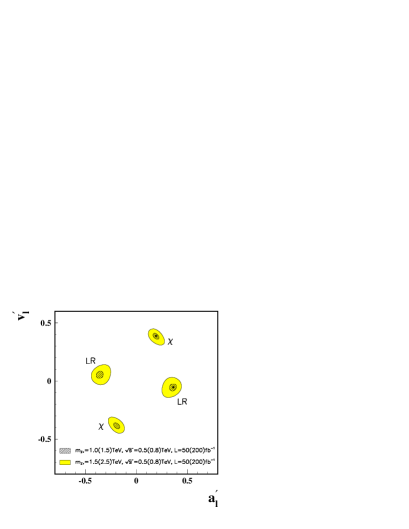
Figure 20: Upper part: $Z^{\prime}$ mass limits in $E_{6}$ and left-right models as a function of the mixing parameters $\cos\beta$ and $\alpha_{LR}$, respectively. Shown are 95% confidence limits based on an integrated luminosity of 20 ${\rm fb}^{-1}$ at a c.m. energy of 500 GeV. The thick solid curve is the result of combining the measurements of $\sigma^{\rm lept},R=\sigma^{\rm had}/\sigma^{\rm lept}$ and $A^{\rm lept}_{FB}$. The thick dotted curve assumes longitudinal polarization and includes the measurement of $A^{\rm had}_{\rm LR}$ and $A^{\rm lept}_{\rm LR}$. The corresponding thin curves include only the effects of statistics. Ref.[90]. Lower part: Resolution power for $M_{Z^{\prime}}=1.5$ TeV at $\sqrt{s}=500$ GeV, 95% CL, for the $E(6)\chi$ and $LR$ models, based on the measurements of leptonic vector and axial charges; Ref.[91].

$s$–channel $Z$ (or $Z^{\prime}$) exchange, so that the cross sections are relatively small. But for the first generation leptons, additional $t$–channel exchanges [$W$ exchange for neutral leptons and $Z$ exchange for charged leptons] are present, increasing the cross sections eventually by several orders of magnitude to a level of $10^{2}$ to $10^{3}$ fb.

Extended gauge theories can lead to additional exciting phenomena which are quite foreign to the observations in the Standard Model . This may be illustrated by two examples. In left-right symmetric theories based on $\rm SO(10)$, heavy Majorana neutrinos may exist. The $t$–channel exchange of these particles can induce the lepton-number violating process

$$e^{-}e^{-}\to W^{-}W^{-}$$

in electron-electron collisions [93], probing Majorana masses up to 20 TeV for neutrino mixings of order $10^{-3}$. The second example in such a scenario is the production of doubly-charged Higgs bosons $\Delta^{--}$ in $e^{-}e^{-}$ collisions [94],

$$e^{-}e^{-}\to\Delta^{--}$$

Additional production channels of this particle, based on the conversion $\gamma\rightarrow e^{-}$ in $e^{-}\gamma$ collisions, are discussed in Ref.[95].

6 The Higgs Mechanism

The Higgs mechanism is the third building block in the electroweak sector of the Standard Model. The fundamental particles, leptons, quarks and weak gauge bosons, acquire masses through the interaction with a scalar field of non-zero field strength in the ground state [3].

To accommodate the well-established electromagnetic and weak phenomena, the Higgs mechanism requires the existence of at least one weak isodoublet scalar field. After absorbing three Goldstone modes to build up the longitudinal polarization states of the $W^{\pm}/Z$ bosons, one degree of freedom is left over, corresponding to a real scalar particle. The discovery of this Higgs boson and the verification of its characteristic properties is crucial for the theory of the electroweak interactions. The physical implications reach far beyond the canonical formulation of the Standard Model.

The only unknown parameter in the Higgs sector of the Standard Model is the mass of the Higgs particle. Stringent constraints however can be derived from the scale $\Lambda$ up to which the Standard Model is assumed to be valid before the gauge and Higgs particles become strongly interacting and new physics phenomena may emerge [96], c.f. Fig.21. The strength of the Higgs self-interaction is determined by the Higgs mass itself at the scale $v=$ 246 GeV, the value of the Higgs field in the ground state which characterizes the spontaneous breaking of the electroweak gauge symmetries. Increasing the energy scale, the quartic self-coupling of the Higgs field increases logarithmically, in a similar way to the electromagnetic coupling in QED. If the Higgs mass is small, the energy cut-off $\Lambda$ at which the coupling grows beyond any given bound, is large; conversely, if the Higgs mass is large, the cut-off $\Lambda$ is small. The condition $M_{H}<\Lambda$ sets an upper limit on the Higgs mass in the Standard Model. It has been shown in lattice analyses, which account properly for the onset of the strong interactions in the Higgs sector, that this condition leads to an estimate of about 700 GeV for the upper limit on $M_{H}$ [98]. [These analyses are based on the orthodox $\Phi^{4}$ formulation of the Standard Model. Therefore, they do not exclude higher values for Higgs masses in any extension of the Standard Model.]

However, if the Higgs mass is less than 180 to 200 GeV, the Standard Model can be extended up to the grand unification scale $\Lambda_{\rm GUT}\sim 10^{16}$ GeV while all particles remain weakly interacting. The hypothesis that interactions between $W/Z$ bosons and Higgs particles remain weak up to the GUT scale, plays a key rôle in explaining the experimental value of the electroweak mixing parameter $\sin^{2}\theta_{w}$. Based on the SM particle spectrum, the electroweak mixing parameter evolves in this scenario from the symmetry value 3/8 at the GUT scale down to $\sim$ 0.2 at ${\cal O}(100$ GeV). Even though additional degrees of freedom are needed to account for the difference from the experimentally observed value 0.23, the hypothesis that the particle interactions remain weak up to the GUT scale is nevertheless strongly supported by this result. From the additional requirement of vacuum stability, lower bounds on the Higgs mass can be derived. Negative loop corrections to the Higgs potential due to heavy top quarks can only be balanced if the Higgs mass is sufficiently large. Based on these arguments, the SM Higgs mass would be expected in the window $130\stackrel{{\scriptstyle<}}{{\sim}}M_{H}\stackrel{{\scriptstyle<}}{{\sim}}180$ GeV for a top mass value of about 175 GeV (c.f. Fig.21). This mass range agrees nicely with the most probable estimate of the Higgs mass from the high-precision electroweak data [99]: $M_{H}=159\stackrel{{\scriptstyle+153}}{{\scriptstyle-86}}$ GeV.

Figure 21: Bounds on the mass of the Higgs boson in the Standard Model. $\Lambda$ denotes the energy scale at which the Higgs-gauge boson system of the Standard Model would become strongly interacting (upper bound); the lower bound follows from the requirement of vacuum stability. Refs.[96, 97].

The SM Higgs boson can be discovered at the LHC in the region above LEP2, including a firm overlap of the two machines, up to the canonical upper limit of $M_{H}\sim 800$ GeV. In the theoretically preferred intermediate mass range below the $ZZ$ decay threshold, the experimental search is difficult.

A large variety of channels can be exploited to search for Higgs particles in the Higgs-strahlung [100, 101] and fusion processes [?–?] at $e^{+}e^{-}$ colliders. The signature is very clear and the background almost negligible so that the properties of the Higgs boson can easily be reconstructed, in particular in the preferred intermediate mass region. In the Higgs-strahlung process $e^{+}e^{-}$ $\to ZH$, recoil-mass techniques can be used in final states with leptonic $Z$ decays, or the Higgs particle may be reconstructed in $H\to b\bar{b},WW$ directly. The $WW$ fusion process $e^{+}e^{-}$ $\to\bar{\nu}_{e}\nu_{e}H$ requires the reconstruction of the Higgs particle.

Once the Higgs boson is found, it will be very important to explore the properties which reveal the physical nature of the particle. The zero-spin of the Higgs particle is reflected in the angular distribution of the Higgs-strahlung process which asymptotically must approach the $\sin^{2}\theta$ law. Of paramount importance is the measurement of the couplings to gauge bosons and matter particles. The strength of the couplings to $Z$ and $W$ bosons is reflected in the size of the $e^{+}e^{-}$ production cross sections. The strength of the couplings to fermions can be measured through the decay branching ratios and Higgs bremsstrahlung off top quarks. These measurements are important instrumentaria to establish the Higgs mechanism experimentally. Finally, the Higgs potential itself, which provides the physical basis of the Higgs phenomenon, must be reconstructed by measuring the triple and quartic Higgs self-couplings [105]. This appears possible only by exploiting multi-Higgs production in the fusion mechanism at TeV energies and maximum possible luminosity.

6.1 Decays of the Higgs Boson

The profile of the Higgs particle is uniquely determined if the Higgs mass is fixed. For Higgs particles in the lower part of the intermediate mass range $M_{Z}\leq M_{H}\leq 2M_{Z}$, the main decay modes [106] are fermion decays, in particular $b\bar{b}$ final states,

$$\Gamma(H\to f\bar{f})=\frac{G_{F}N_{C}}{4\sqrt{2}\pi}m_{f}^{2}(M_{H}^{2})M_{H}$$ (15)

and in the upper part WW and $ZZ$ pairs with one of the two gauge bosons being virtual below the threshold,

$$\Gamma(H\to VV)=\frac{3G_{F}^{2}M_{Z}^{4}}{16\pi^{3}}M_{H}R_{V}(M_{V}^{2}/M_{H}^{2})\to 2(1)\frac{\sqrt{2}G_{F}}{32\pi}M_{H}^{3}\;\;\hskip 5.69054pt[V=W(Z)]$$ (16)

Figure 22: Branching ratios of the main decay modes of the SM Higgs boson and total decay width; Ref.[106].

Above the WW threshold, the Higgs particles decay almost exclusively into the $W/Z$ channels, except in the mass range near the $t\bar{t}$ decay threshold. Below 140 GeV, the decays $H\to\tau^{+}\tau^{-},c\bar{c}$ and $gg$ are also important besides the dominating $b\bar{b}$ channel. By adding up all possible decay channels, we obtain the total Higgs decay width shown in Fig.22 for $m_{t}=$ 175 GeV. Up to masses of 140 GeV, the Higgs particle is very narrow, $\Gamma(H)\leq$ 10 MeV. After opening the mixed real/virtual gauge boson channels, the state becomes rapidly wider, reaching $\sim$ 1 GeV at the $ZZ$ threshold. The width cannot be measured directly in the intermediate mass range. Only above $M_{H}\geq$ 200 GeV it becomes wide enough to be resolved experimentally.

6.2 The Production of Higgs Bosons

The main production mechanism for Higgs particles of moderate mass and at moderate energies in $e^{+}e^{-}$ collisions is the Higgs-strahlung off the $Z$ boson line [100, 101]

$$e^{+}e^{-}\stackrel{{\scriptstyle Z}}{{\longrightarrow}}ZH$$

The cross section is given by

$$\sigma(e^{+}e^{-}\to ZH)=\frac{G_{F}^{2}M_{Z}^{4}}{96\pi s}(v_{e}^{2}+a_{e}^{2})\lambda^{\frac{1}{2}}\frac{\lambda+12M_{Z}^{2}/s}{(1-M_{Z}^{2}/s)^{2}}$$ (17)

where $\lambda$ is the usual 2–body phase space coefficient. For a given Higgs mass $M_{H}$, the Higgs-strahlung cross section is maximal for the c.m. energy $\sqrt{s}\sim M_{Z}+2M_{H}$. Beyond the threshold region, the cross section for Higgs-strahlung scales as $s^{-1}$ and vanishes asymptotically. With rising energy the fusion mechanisms, in particular WW fusion, become increasingly important [?–?],

$$e^{+}e^{-} \stackrel{{\scriptstyle WW}}{{\longrightarrow}} \bar{\nu}_{e}\nu_{e}H$$

$$e^{+}e^{-} \stackrel{{\scriptstyle ZZ}}{{\longrightarrow}} e^{+}e^{-}H$$

The corresponding cross sections rise logarithmically with energy; for WW fusion:

$$\sigma(e^{+}e^{-}\to\bar{\nu}_{e}\nu_{e}H)\to\frac{G_{F}^{3}M_{W}^{4}}{4\sqrt{2}\pi^{3}}\left[\left(1+\frac{M_{H}^{2}}{s}\right)\log\frac{s}{M_{H}^{2}}-2\left(1-\frac{M_{H}^{2}}{s}\right)\right]$$ (18)

Due to the reduced $Z$ charges, the cross section for $ZZ$ fusion is about one order of magnitude smaller; the same applies for $ZZ$ fusion in $e^{-}e^{-}$ collisions. However, with two leptons in the final states, recoil mass techniques can be applied which allow a more effective background rejection compared to the neutrino channel.

The cross sections for the Higgs-strahlung process and the fusion processes are shown in Fig.23 for $\sqrt{s}=500$ and 800 GeV. Several thousand events will be produced for the envisaged luminosities.

Figure 23: The cross section for the production of SM Higgs bosons in Higgs-strahlung $e^{+}e^{-}\rightarrow ZH$ and $WW/ZZ$ fusion $e^{+}e^{-}\rightarrow\overline{\nu}\nu/e^{+}e^{-}H$; solid curves: $\sqrt{s}=500$ GeV, dashed curves: $\sqrt{s}=800$ GeV.

The recoiling $Z$ boson in the two-body reaction $e^{+}e^{-}\to ZH$ is mono-energetic and the Higgs mass can be derived from the energy of the $Z$ boson, $M_{H}^{2}=s-2\sqrt{s}E_{Z}+M_{Z}^{2}$. The detection of the Higgs boson in this channel is independent of the Higgs decay properties, thus providing a very powerful tool for the search of this particle. Initial-state bremsstrahlung and beamstrahlung smear out the peak slightly [107]. $ZZ$ production does not pose a serious background problem; if efficient $b$ tagging devices are used, the Higgs signal can be extracted even for masses close to the $Z$ mass [108]. Signal and background are shown in Fig.24. A similar clear peak can be observed in the fusion process $e^{+}e^{-}\to\bar{\nu_{e}}\nu_{e}H$ by collecting the decay products of the Higgs boson. The dominant background process in this case is the reaction $e^{+}e^{-}\to(e^{+})\nu_{e}W^{-}$, with the final state positron traveling undetected along the beam pipe; this background is negligible also with experimental resolution effects taken into account.

Figure 24: Dilepton recoil mass analysis of Higgs-strahlung $e^{+}e^{-}\rightarrow ZH\rightarrow l^{+}l^{-}+\rm{anything}$ in the intermediate Higgs mass range for $M_{H}=140$ GeV. The c.m. energy is $\sqrt{s}$=360 GeV and the integrated luminosity $\int{\cal L}=$50 fb^-1. Ref.[109].

6.3 Higgs Production in $\gamma\gamma$ Collisions

The production of Higgs bosons in $\gamma\gamma$ collisions [110] can be exploited to determine important properties of these particles, in particular the two-photon width. The $H\gamma\gamma$ coupling is built up by loops of charged particles. If the mass of the loop particle is generated through the Higgs mechanism, the decoupling of the heavy particles is lifted and the $\gamma\gamma$ width reflects the spectrum of these states with masses possibly far above the Higgs mass.

Together with the measurement of the branching ratio $BR_{\gamma\gamma}$ at the LHC, or if enough events can be generated at $e^{+}e^{-}$ linear colliders in Higgs-strahlung, the measurement of the $\gamma\gamma$ partial width can be used to determine the total width of the Higgs boson in a range where it cannot be resolved experimentally.

The two-photon width is related to the $\gamma\gamma$ production cross section by

$$\sigma(\gamma\gamma_{J_{z}=0}\rightarrow H)=\frac{16\pi^{2}\Gamma(H\rightarrow\gamma\gamma)}{M_{H}}\times BW$$ (19)

where $BW$ denotes the Breit–Wigner resonance factor in terms of the energy squared. For narrow Higgs bosons the observed cross section is found by folding the parton cross section with the invariant $\gamma\gamma$ energy flux $\tau d{\cal L}^{\gamma\gamma}/d\tau$ for $J_{z}^{\gamma\gamma}=0$ at $\tau=M_{H}^{2}/s_{ee}$.

The event rate for the production of Higgs bosons in $\gamma\gamma$ collisions of Weizsäcker–Williams photons is too small to play a rôle in practice. However, the rate is sufficiently large if the photon spectra are generated by Compton back-scattering of laser light, Fig.25; the $\gamma\gamma$ luminosity in such a Compton collider is expected to be only slightly smaller than the luminosity in $e^{+}e^{-}$ collisions. In the Higgs mass range between 100 and 150 GeV, the final state consists primarily of $b\overline{b}$ pairs. The large $\gamma\gamma$ continuum background is suppressed in the $J_{z}^{\gamma\gamma}=0$ polarization state. For Higgs masses above 150 GeV, $WW$ final states become dominant, supplemented in the ratio 1:2 by $ZZ$ final states above the $ZZ$ decay threshold. While the continuum $WW$ background in $\gamma\gamma$ collisions is very large, the $ZZ$ background appears under control for masses up to order 300 GeV [111]. The error on the partial $\gamma\gamma$ decay width of the Higgs boson is expected in the range of 10% [110, 112].

Additional sources of Higgs bosons are provided by $e\gamma$ collisions [113]. The process $e\gamma\rightarrow\nu WH$ is generated at the tree level while Higgs production in $e\gamma\rightarrow eH$ proceeds through the fusion of the real and virtual photon. For $\sqrt{s}=500$ GeV the cross sections are larger than 10 fb for Higgs masses below 250 GeV. For $\sqrt{s}=800$ GeV, this limit is raised to 450 GeV in the $\nu WH$ process, with an initial cross section of 100 fb for a Higgs mass of 100 GeV.

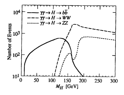
Figure 25: Production rate of Standard Model Higgs bosons into the three exclusive final states relevant for the intermediate– and heavy mass regions in ${\gamma\gamma}$ collisions. A value of $4\cdot 10^{-2}\rm{fb}^{-1}/\rm{GeV}$ is assumed for $d{\cal L}^{\gamma\gamma}/dW_{\gamma\gamma}$. Ref.[110].

6.4 The Profile of the Higgs Particle

To establish the Higgs mechanism experimentally, the nature of this particle must be explored by measuring all its characteristics, the mass and lifetime, the external quantum numbers spin-parity, the couplings to gauge bosons and fermions, and last but not least the self-couplings. This program can be realized at $e^{+}e^{-}$  colliders in consecutive steps.

The mass of the Higgs particle can be determined at $e^{+}e^{-}$ linear colliders very precisely. This can be achieved by exploiting the kinematical constraints in the four-jet topology, the $\tau\bar{\tau}q\bar{q}$ final state and the leptonic channels in Higgs-strahlung events [114]. For an integrated luminosity $\int{\cal{L}}=$ 50 fb^-1 at $\sqrt{s}=500$ GeV, a precision of $\pm 180$ MeV can be reached; at this level, systematic errors due to the measurement of the beam energy can still be neglected.

The width of the state, i.e. the lifetime of the particle, can be measured directly above the $ZZ$ decay threshold where the width grows rapidly. In the lower part of the intermediate mass range the width can be measured indirectly by combining the branching ratio for $H\to\gamma\gamma$, accessible at the LHC, with the measurement of the partial $\gamma\gamma$ width, accessible through $\gamma\gamma$ production at a Compton collider. In the upper part of the intermediate mass range, the combination of the branching ratios for $H\to WW,ZZ$ decays with the production cross sections for WW  fusion and Higgs-strahlung, which can be expressed both through the partial Higgs-decay widths to WW and $ZZ$ pairs, will allow us to extract the width of the Higgs particle. Thus, the width of the Higgs particle will be determined throughout the entire possible mass range if the experimental results from LHC, $e^{+}e^{-}$ and optional $\gamma\gamma$ colliders can be combined.

The angular distribution of the $Z/H$ bosons in the Higgs-strahlung process is sensitive to the spin and parity of the Higgs particle [101]. Since the production amplitude is given by ${\cal A}(0^{+})\sim\vec{\varepsilon_{Z^{*}}}\cdot\vec{\varepsilon_{Z}}$, the $Z$ boson is produced in a state of longitudinal polarization at high energies – in accord with the equivalence theorem. As a result, the angular distribution

$$d\sigma/d\cos\theta\sim\sin^{2}\theta+8M_{Z}^{2}/(\lambda s)$$ (20)

approaches the spin-zero $\sin^{2}\theta$ law asymptotically. This may be contrasted with the distribution $\sim 1+\cos^{2}\theta$ for negative parity states which follows from the transverse polarization amplitude ${\cal A}(0^{-})\sim\vec{\varepsilon_{Z^{*}}}\times\vec{\varepsilon_{Z}}\cdot\vec{k_{Z}}$. It is also characteristically different from the distribution of the background process $e^{+}e^{-}\to ZZ$ which, as a result of $t/u$–channel $e$ exchange, is strongly peaked in the forward/backward direction, Fig.26.

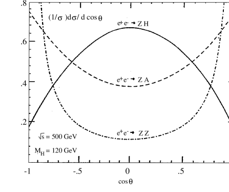
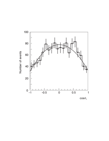
Figure 26: Left: Angular distribution of $Z/H$ bosons in Higgs-strahlung, compared with the production of pseudoscalar particles and the $ZZ$ background final states; Ref.[101]. Right: The same for the signal plus background in the experimental simulation of Ref.[114].

Since the fundamental particles acquire masses through the interaction with the Higgs field, the strength of the Higgs couplings to fermions and gauge bosons is set by the masses of these particles. It will therefore be a very important task to measure the Higgs couplings to the fundamental particles, which are uniquely predicted by the very nature of the Higgs mechanism. The Higgs couplings to massive gauge bosons can be determined from the production cross sections with an accuracy of $\pm 3$ %, the $HZZ$ coupling in the Higgs-strahlung and the $HWW$ coupling in the fusion process. For Higgs couplings to fermions, either loop effects in $H\rightleftharpoons gg,\gamma\gamma$ [mediated by top quarks] must be exploited, or the branching ratios $H\to b\bar{b},c\bar{c},\tau^{+}\tau^{-}$ in the lower part of the intermediate mass range; they provide a direct determination of the Higgs Yukawa couplings to these fermions. This is exemplified for a Higgs mass of 140 GeV in Fig.27.

The Yukawa coupling of the intermediate Higgs boson to the top quark in the range $M_{H}\leq$ 120 GeV can be measured directly in the bremsstrahlung process $e^{+}e^{-}\to t\bar{t}H$ in which primarily the top quarks radiate the Higgs boson in high energy $e^{+}e^{-}$  collisions [117]. Since the top quark is very heavy, the $ttH$ coupling may eventually provide essential clues to the nature of the mechanism breaking the electroweak symmetries. Even though the experiment is difficult due to the small cross section, Fig.28, and the complex topology of the $bbbbWW$ final state, this analysis is an important experimental task to explore the electroweak symmetry breaking. For large Higgs masses above the $t\bar{t}$ threshold, the decay channel $H\to t\bar{t}$ increases the cross section of $e^{+}e^{-}\to t\bar{t}Z$ through the reaction $e^{+}e^{-}\to ZH(\to t\bar{t})$ [118]. Higgs exchange between $t\bar{t}$ quarks also affects the excitation curve near the threshold at a level of a few percent.

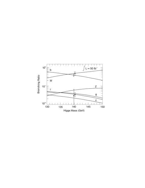
Figure 27: The measurement of decay branching ratios of the SM Higgs boson for $M_{H}=140$ GeV. In the bottom part of the figure the small error bar belongs to the $\tau$ branching ratio, the large bar to the sum of the charm and gluon branching ratios which were not separated in the simulation of Ref.[115]. In the upper part of the figure the open circle denotes the $b$ branching ratio, the full circle the $W$ branching ratio.

Figure 28: The cross section for bremsstrahlung of SM Higgs bosons off top quarks in the Yukawa process $e^{+}e^{-}\to t\bar{t}H$. [The amplitude for radiation off the intermediate $Z$–boson line is small]; Ref.[117].

The Higgs mechanism, based on a non-zero value of the Higgs field in the vacuum, must finally be made manifest experimentally by reconstructing the interaction potential which generates the non-zero Higgs field in the vacuum. This program can be carried out by measuring the strength of the trilinear and quartic self-couplings of the Higgs particles. This is a very difficult task since the processes to be exploited are suppressed by small couplings and phase space. Nevertheless, the problem can be solved in the high energy phase of the $e^{+}e^{-}$  linear colliders for sufficiently high luminosities [105]. The best suited reaction for the measurement of the trilinear coupling for Higgs masses in the theoretically preferred ${\cal O}(100$ GeV) mass range, is the $WW$ fusion process

$$e^{+}e^{-}\to\bar{\nu}_{e}\nu_{e}HH$$

in which, among other mechanisms, the two-Higgs final state is generated by the $s$–channel exchange of a virtual Higgs particle so that this process is sensitive to the trilinear $HHH$ coupling in the Higgs potential. Since the cross section is only a fraction of 1 fb at an energy of $\sim$ 1.6 TeV, an integrated luminosity of $\sim 1,000$ fb^-1 is needed to isolate the events. The quartic coupling $H^{4}$ seems to be accessible only through loop effects in the foreseeable future.

To sum up, we conclude from the preceding discussion that $e^{+}e^{-}$ linear colliders with energies in the range of 300 to 500 GeV are the ideal instruments to search for Higgs particles in the intermediate mass range, a priori the theoretically most attractive range, and to establish its characteristic properties experimentally. In the high energy phase of the colliders, important parameters of the Higgs potential can be reconstructed which are necessary for generating the spontaneous breaking of the electroweak symmetries.

7 Supersymmetry

Even though no direct experimental evidence has emerged yet for the existence of supersymmetry [5] in Nature, the concept has so many attractive features that it may be considered as a prime target of present and future experimental particle research. Arguments in favor of supersymmetry are deeply rooted in particle physics. Supersymmetry unifies matter and forces, and if realized locally, it plays a crucial r$\hat{\rm o}$le in a quantum theory of gravity. In relating particles of different spins to each other, fermions and bosons, low-energy supersymmetry stabilizes the masses of fundamental Higgs scalars in the context of very high energy scales associated with grand unification [119]. Besides solving this part of the hierarchy problem, supersymmetry may even be closely related to the physical origin of the Higgs mechanism itself [120]: In supergravity inspired realizations of supersymmetric theories [121], incorporating universal scalar masses at the scale of the grand unification, one of the scalar masses squared can evolve down to negative values and thus induce spontaneous symmetry breaking in the electroweak sector. This is possible if the top mass has a value between 150 and 200 GeV; all other masses squared of squarks and sleptons remain positive so that ${\rm U}(1)_{EM}$ and ${\rm SU}(3)_{C}$ are unbroken.

The minimal supersymmetric extension of the Standard Model [122], MSSM, is based on the symmetry group $\rm SU(3)\times SU(2)\times U(1)$ of the Standard Model. The gauginos are the supersymmetric spin–$\frac{1}{2}$ partners of the gauge bosons. The matter particles, quarks and leptons, are associated with scalar supersymmetric particles, squarks and sleptons. To preserve supersymmetry and to keep the theory free of anomalies, two Higgs doublets are needed, the supersymmetric partners of which are spin–$\frac{1}{2}$ higgsinos. Charged/neutral higgsinos mix in general with the non-colored gauginos, forming charginos and neutralinos. Supersymmetric partners carry a multiplicative quantum number $R=-1$ [$R=+1$ for ordinary particles] which is conserved in this model. Supersymmetric particles are therefore generated in pairs and the lightest supersymmetric particle ($LSP$) is stable. This particle is in general identified with the lightest neutralino, but it could also be the sneutrino.

Strong support for supersymmetry and the particle spectrum of the minimal supersymmetric standard model in the mass range of several hundred GeV follows from the high-precision measurement of the electroweak mixing angle $\sin^{2}\theta_{w}$ [123, 124]. The value predicted by the MSSM, $\sin^{2}\theta_{w}=0.2336\pm 0.0017$, is matched surprisingly well by the value determined by the LEP and other experiments, $\sin^{2}\theta_{w}=0.2315\pm 0.0003$, the theoretical uncertainty being less than 2 permille.

In the simplest realization of supersymmetric grand unified theories, with the supersymmetry breaking parameters taken to be universal at the GUT scale, five parameters specify the supersymmetric particle sector. They can be chosen as the (universal) scalar mass parameter $m_{0}$; the (universal) gaugino mass $M_{1\!/\!2}$; $\tan\beta$, the ratio of the vacuum expectation values $v_{2}/v_{1}$ associated with the two neutral Higgs fields; the (universal) trilinear scalar coupling $A_{0}$; and the sign of $\mu$, the Higgs mass parameter in the superpotential. Evolving the universal mass parameters from the GUT scale down to the electroweak scale, the entire spectrum of the Higgs particles and the supersymmetric particles can be generated, see, for example, the analysis in Ref.[125]. It is well-known that the mass of the lightest Higgs particle is less than about 150 GeV in the MSSM; this bound follows from the fact that the quartic couplings are given by the gauge couplings. The non-colored particles, charginos/neutralinos and sleptons, are in general significantly lighter than colored particles in this scenario. The lightest of these particles can have masses in the range of 100 to 200 GeV.

This general discussion is quantified in Table 4 for a few illustrative examples. The input parameters [$m_{0},M_{1\!/\!2},A_{0},\tan\beta,{\rm sgn}\ \mu$] have been chosen such that they are compatible with constraints on the low-energy MSSM from the $b\to s\gamma$ decays [126], demanding $1\cdot 10^{-4}<{\rm BR}(b\to s\gamma)<4\cdot 10^{-4}$. Moreover, cosmological constraints are taken into account by requiring the matter density in the universe, primarily composed of relic neutralinos, to be bounded as predicted in the mixed hot/cold dark matter scenario, $\Omega h^{2}\sim 0.15$ to 0.4, or more generally, by $\Omega h^{2}<1$ as required by the age of the universe [127]. The mass parameters have been computed within the approximate solutions of Refs.[128, 129]. The particles of Table 4 which are accessible at a c.m. energy of $\sqrt{s}=500$ GeV are marked by one asterisk, the particles which are accessible at 1 TeV, by two asterisks. All other particles in the table can be produced at a c.m. energy of about 2 TeV. The range of the masses is illustrated for the two points B and G in Fig.29.

Figure 29: Illustration of supersymmetric particle masses in two typical points of the parameter space of minimal supergravity.

7.1 SUSY Higgs Particles

One of the prime arguments for introducing supersymmetry is the solution of the hierarchy problem. By assigning fermions and bosons to common multiplets, large radiative corrections can be canceled in a natural way [119] by adding up bosonic and

Point	A	B	C	D	E	F	G
SGUT Parameters
$m_{0}$	125	200	125	200	100	200	260
$M_{1\!/\!2}$	175	100	175	400	200	400	220
$A_{0}$	0	0	0	0	0	0	-500
$\tan\beta$	2	2	2	10	10	10	1.6
${\rm sgn}(\mu)$	–	–	+	–	+	+	+
Mass Parameters
$h^{0}$	74${}^{\hskip 2.84526pt*}$	68${}^{\hskip 2.84526pt*}$	86${}^{\hskip 2.84526pt*}$	114${}^{\hskip 2.84526pt*}$	110${}^{\hskip 2.84526pt*}$	116${}^{\hskip 2.84526pt*}$	101${}^{\hskip 2.84526pt*}$
$A^{0}$	433${}^{\hskip 2.84526pt**}$	367${}^{\hskip 2.84526pt**}$	434${}^{\hskip 2.84526pt**}$	660	321${}^{\hskip 2.84526pt**}$	660	765
$H^{0}$	438${}^{\hskip 2.84526pt**}$	373${}^{\hskip 2.84526pt**}$	439${}^{\hskip 2.84526pt**}$	660	321${}^{\hskip 2.84526pt**}$	661	769
$H^{\pm}$	440${}^{\hskip 2.84526pt**}$	374${}^{\hskip 2.84526pt**}$	440${}^{\hskip 2.84526pt**}$	665	330${}^{\hskip 2.84526pt**}$	665	769
$\tilde{\chi_{1}^{0}}$	75${}^{\hskip 2.84526pt*}$	44${}^{\hskip 2.84526pt*}$	64${}^{\hskip 2.84526pt*}$	164${}^{\hskip 2.84526pt*}$	78${}^{\hskip 2.84526pt*}$	163${}^{\hskip 2.84526pt*}$	88${}^{\hskip 2.84526pt*}$
$\tilde{\chi_{2}^{0}}$	151${}^{\hskip 2.84526pt*}$	95${}^{\hskip 2.84526pt*}$	122${}^{\hskip 2.84526pt*}$	321${}^{\hskip 2.84526pt*}$	144${}^{\hskip 2.84526pt*}$	315${}^{\hskip 2.84526pt*}$	171${}^{\hskip 2.84526pt*}$
$\tilde{\chi_{3}^{0}}$	352${}^{\hskip 2.84526pt*}$	259${}^{\hskip 2.84526pt*}$	350${}^{\hskip 2.84526pt*}$	579${}^{\hskip 2.84526pt**}$	289${}^{\hskip 2.84526pt*}$	577${}^{\hskip 2.84526pt**}$	552${}^{\hskip 2.84526pt**}$
$\tilde{\chi_{4}^{0}}$	364${}^{\hskip 2.84526pt*}$	276${}^{\hskip 2.84526pt*}$	378${}^{\hskip 2.84526pt*}$	585${}^{\hskip 2.84526pt**}$	313${}^{\hskip 2.84526pt*}$	591${}^{\hskip 2.84526pt**}$	571${}^{\hskip 2.84526pt**}$
$\tilde{\chi_{1}^{\pm}}$	151${}^{\hskip 2.84526pt*}$	94${}^{\hskip 2.84526pt*}$	119${}^{\hskip 2.84526pt*}$	321${}^{\hskip 2.84526pt**}$	142${}^{\hskip 2.84526pt*}$	315${}^{\hskip 2.84526pt**}$	170${}^{\hskip 2.84526pt*}$
$\tilde{\chi_{2}^{\pm}}$	363${}^{\hskip 2.84526pt*}$	275${}^{\hskip 2.84526pt*}$	375${}^{\hskip 2.84526pt*}$	588${}^{\hskip 2.84526pt**}$	314${}^{\hskip 2.84526pt*}$	591${}^{\hskip 2.84526pt**}$	567${}^{\hskip 2.84526pt**}$
$\tilde{l_{R}}$	146${}^{\hskip 2.84526pt*}$	207${}^{\hskip 2.84526pt*}$	146${}^{\hskip 2.84526pt*}$	257${}^{\hskip 2.84526pt*/}$	134${}^{\hskip 2.84526pt*}$	257${}^{\hskip 2.84526pt*/}$	275${}^{\hskip 2.84526pt**}$
$\tilde{l_{L}}$	181${}^{\hskip 2.84526pt*}$	216${}^{\hskip 2.84526pt*}$	181${}^{\hskip 2.84526pt*}$	354${}^{\hskip 2.84526pt**}$	182${}^{\hskip 2.84526pt*}$	354${}^{\hskip 2.84526pt**}$	305${}^{\hskip 2.84526pt**}$
$\tilde{\nu_{L}}$	170${}^{\hskip 2.84526pt*}$	207${}^{\hskip 2.84526pt*}$	170${}^{\hskip 2.84526pt*}$	345${}^{\hskip 2.84526pt**}$	163${}^{\hskip 2.84526pt*}$	345${}^{\hskip 2.84526pt**}$	300${}^{\hskip 2.84526pt**}$
$\tilde{u_{R}}$	403${}^{\hskip 2.84526pt**}$	303${}^{\hskip 2.84526pt**}$	403${}^{\hskip 2.84526pt**}$	817	443${}^{\hskip 2.84526pt**}$	817	550
$\tilde{u_{L}}$	415${}^{\hskip 2.84526pt**}$	307${}^{\hskip 2.84526pt**}$	415${}^{\hskip 2.84526pt**}$	850	457${}^{\hskip 2.84526pt**}$	850	566
$\tilde{d_{R}}$	402${}^{\hskip 2.84526pt**}$	304${}^{\hskip 2.84526pt**}$	402${}^{\hskip 2.84526pt**}$	813	442${}^{\hskip 2.84526pt**}$	813	549
$\tilde{d_{L}}$	419${}^{\hskip 2.84526pt**}$	313${}^{\hskip 2.84526pt**}$	419${}^{\hskip 2.84526pt**}$	853	463${}^{\hskip 2.84526pt**}$	853	569
$\tilde{b_{1}}$	376${}^{\hskip 2.84526pt**}$	268${}^{\hskip 2.84526pt**}$	376${}^{\hskip 2.84526pt**}$	766	420${}^{\hskip 2.84526pt**}$	766	492${}^{\hskip 2.84526pt**}$
$\tilde{b_{2}}$	402${}^{\hskip 2.84526pt**}$	304${}^{\hskip 2.84526pt**}$	402${}^{\hskip 2.84526pt**}$	811	445${}^{\hskip 2.84526pt**}$	811	550
$\tilde{t_{1}}$	339${}^{\hskip 2.84526pt**}$	258${}^{\hskip 2.84526pt*/}$	252${}^{\hskip 2.84526pt*/}$	611	325${}^{\hskip 2.84526pt**}$	598	305${}^{\hskip 2.84526pt**}$
$\tilde{t_{2}}$	415${}^{\hskip 2.84526pt**}$	311${}^{\hskip 2.84526pt**}$	473${}^{\hskip 2.84526pt**}$	823	505${}^{\hskip 2.84526pt**/}$	832	594
$\tilde{g}$	459${}^{\hskip 2.84526pt**}$	291${}^{\hskip 2.84526pt**}$	460${}^{\hskip 2.84526pt**}$	953	515	953	584

Table 4: Typical mass spectra of supersymmetric particles derived from various sets of supergravity parameters. Particles with one asterisk can be produced at collider energies of $\sqrt{s}=500$ GeV, with two asterisks at 1 TeV; all the particles can be produced at about 2 TeV. [Particles which are located just at the borderline between two collider energies, are characterized by oblique strokes.]

opposite-sign fermionic loops. As a result of the bosonic-fermionic supersymmetry, Higgs bosons can be retained as elementary spin-zero particles with masses close to the scale of the electroweak symmetry breaking even in the context of very high grand unification scales. The minimal supersymmetric extension of the Standard Model serves as a useful guideline into this area. Only a few phenomena are specific to this minimal version, many of the characteristic patterns are realized also in more general extensions. High-energy $e^{+}e^{-}$ colliders can easily cope with the experimental problems in such general scenarios since methods of analysis appropriate to these machines are quite robust, and do not rely upon specific favorable circumstances.

The Higgs spectrum in the MSSM consists of five particles [130, 131], $h^{0},H^{0},A^{0}$ and $H^{\pm}$, the states $h^{0},H^{0}$ and $A^{0}$ being ${\cal CP}$ even and odd, respectively. Besides the masses, two mixing angles define the properties of the scalar particles and their interactions with gauge bosons and fermions: the ratio of the two vacuum expectation values $\tan\beta=v_{2}/v_{1}$ and a mixing angle $\alpha$ in the neutral ${\cal CP}$–even sector. Supersymmetry leads to several relations among these parameters and, in fact, only two of them are independent. These relations impose, at the tree-level, a strong hierarchical structure on the mass spectrum $[M_{h}<M_{Z},M_{A}<M_{H}$ and $M_{W}<M_{H^{\pm}}]$ which however is broken by radiative corrections $\sim G_{F}m_{t}^{4}\log{\tilde{m}_{t}^{2}/m_{t}^{2}}$ for the large top quark mass [132] (c.f. Fig.30).

Figure 30: The masses of the Higgs bosons in the Minimal Supersymmetric Standard Model MSSM for two representative values of $\tan\beta=1.5$ and 30.

The couplings of the neutral Higgs bosons to fermions and gauge bosons will in general depend on the angles $\alpha$ and $\beta$. The pseudoscalar boson $A^{0}$ does not have tree-level couplings to gauge bosons, and its couplings to (up) down type fermions are (inversely) proportional to $\tan\beta$. The couplings are in general strongly dependent on the input parameter $\tan\beta$ and the masses. The couplings to down (up) type fermions are enhanced (suppressed) compared to the SM Higgs couplings. If $M_{h}$ is very close to its upper limit for a given value of $\tan\beta$, the couplings to fermions and gauge bosons are SM like; this decoupling limit [133] is realized if the pseudoscalar mass $M_{A}$ exceeds 300 GeV.

a) Decays

The lightest neutral Higgs boson $h^{0}$ will decay mainly into fermion pairs since its mass is smaller than $\sim$ 130 GeV, Fig.31 (c.f. Ref.[134] for a comprehensive summary). This is, in general, also the dominant decay mode of the pseudoscalar boson $A^{0}$. For values of $\tan\beta$ larger than unity and for masses less than $\sim$ 140 GeV, the main decay modes of the neutral Higgs bosons are decays into $b\bar{b}$ and $\tau^{+}\tau^{-}$ pairs; the branching ratios are of order $\sim 90\%$ and $8\%$, respectively. The decays into $c\bar{c}$ pairs and gluons are suppressed especially for large $\tan\beta$. For large masses, the top decay channels $H^{0},A^{0}\rightarrow t\bar{t}$ open up; yet for large $\tan\beta$ this mode remains suppressed and the neutral Higgs bosons decay almost exclusively into $b\bar{b}$ and $\tau^{+}\tau^{-}$ pairs. If the mass is high enough, the heavy ${\cal CP}$–even Higgs boson $H^{0}$ can in principle decay into weak gauge bosons, $H^{0}\to WW,ZZ$. Since the partial widths are proportional to $\cos^{2}(\beta-\alpha)$, they are strongly suppressed in general, and the gold-plated $ZZ$ signal of the heavy Higgs boson in the Standard Model is lost in the supersymmetric extension. As a result, the total widths of the Higgs bosons are much smaller in supersymmetric theories than in the Standard Model, c.f. Fig.32

The heavy neutral Higgs boson $H^{0}$ can also decay into two lighter Higgs bosons. Other possible channels are Higgs cascade decays and decays into supersymmetric particles [?–?], Fig.33. In addition to light sfermions, Higgs boson decays into charginos and neutralinos could eventually be important. These new channels are kinematically accessible at least for the heavy Higgs bosons $H^{0},A^{0}$ and $H^{\pm}$; in fact, the branching fractions can be very large and they can become dominant in some regions of the MSSM parameter space. Decays of $h^{0}$ into the lightest neutralinos $(LSP)$ are also important, exceeding 50% in some parts of the SUSY parameter space. These decays strongly affect experimental search techniques. In particular, neutral Higgs decays into the $LSP$ which would be invisible, could jeopardize the search for the Higgs particles at hadron colliders where these decay modes are very difficult to detect. At $e^{+}e^{-}$ colliders however, missing mass techniques allow us to find these events easily; this is most obvious for the ${\cal CP}$–even Higgs bosons which can be produced in association with the $Z$ boson.

Figure 31: Branching ratios of the main decay modes of the five MSSM Higgs bosons to SM particles and in cascade decays for $\tan\beta=1.5$; Refs.[134, 136].

Figure 32: Total SM plus cascade decay widths of the five MSSM Higgs bosons for $\tan\beta=1.5$.

Figure 33: Decays of MSSM Higgs bosons to charginos/neutralinos and sfermions; Ref.[134, 136].

The charged Higgs particles decay into fermions but also, if allowed kinematically, into the lightest neutral Higgs and a $W$ boson. Below the $tb$ and $Wh$ thresholds, the charged Higgs particles will decay mostly into $\tau\nu_{\tau}$ and $c\bar{s}$ pairs, the former being dominant for $\tan\beta>1$. For large $M_{H^{\pm}}$ values, the top-bottom decay mode $H^{+}\to t\bar{b}$ becomes dominant. In some parts of the SUSY parameter space, decays into supersymmetric particles may exceed 50 percent.

Adding up the various decay modes, the width of all five Higgs bosons remains very narrow, being of order 10 GeV even for large masses.

b) Production

The search for the neutral SUSY Higgs bosons at $e^{+}e^{-}$ colliders will be a straightforward extension of the search performed at LEP2, which is expected to cover the mass range up to $\sim 90\ \makebox{to}\ 100$ GeV for neutral Higgs bosons, depending on $\tan\beta$. Higher energies, $\sqrt{s}$ in excess of $250$ GeV, are required to sweep the entire parameter space of the MSSM.

The main production mechanisms of neutral Higgs bosons at $e^{+}e^{-}$ colliders [131, 136, 138] are the Higgs-strahlung process and associated pair production, as well as the fusion processes:

$$(a)\ \ {\rm Higgs-strahlung}\hskip 28.45274pte^{+}e^{-} \stackrel{{\scriptstyle Z}}{{\longrightarrow}} Z+h/H\hskip 142.26378pt$$

$$(b)\ \ {\rm Pair\ Production}\hskip 38.69576pte^{+}e^{-} \stackrel{{\scriptstyle Z}}{{\longrightarrow}} A+h/H$$

$$(c)\ \ {\rm Fusion\ Processes}\hskip 30.44443pt\ e^{+}e^{-} \stackrel{{\scriptstyle WW}}{{\longrightarrow}} \overline{\nu_{e}}\ \nu_{e}\ +h/H\hskip 93.89418pt$$

$$e^{+}e^{-} \stackrel{{\scriptstyle ZZ}}{{\longrightarrow}} e^{+}e^{-}+h/H$$

The ${\cal CP}$–odd Higgs boson $A^{0}$ cannot be produced in fusion processes to leading order. The cross sections for the four Higgs-strahlung and pair production processes can be expressed as

$$\sigma(e^{+}e^{-}\to Z+h/H) = \sin^{2}/\cos^{2}(\beta-\alpha)\ \sigma_{SM}$$

$$\sigma(e^{+}e^{-}\to A+h/H) = \cos^{2}/\sin^{2}(\beta-\alpha)\ \bar{\lambda}\ \sigma_{SM}$$ (21)

where $\sigma_{SM}$ is the SM cross section for Higgs-strahlung and the coefficient $\bar{\lambda}\sim\lambda^{3/2}_{Aj}/\lambda^{1\!/\!2}_{Zj}$ accounts for the suppression of the $P$–wave $Ah/H$ cross sections near the threshold.

The cross sections for the Higgs-strahlung and for the pair production, likewise the cross sections for the production of the light and the heavy neutral Higgs bosons $h^{0}$ and $H^{0}$, are mutually complementary to each other, coming either with coefficients $\sin^{2}(\beta-\alpha)$ or $\cos^{2}(\beta-\alpha)$. As a result, since $\sigma_{SM}$ is large, at least the lightest ${\cal CP}$–even Higgs boson must be detected.

Figure 34: Production cross sections of MSSM Higgs bosons at $\sqrt{s}=500$ GeV: Higgs-strahlung and pair production; upper part: neutral Higgs bosons, lower part: charged Higgs bosons. Ref.[134].

Representative examples of the cross sections for the production mechanisms of the neutral Higgs bosons are shown as a function of the Higgs masses in Fig.34 for $\tan\beta=1.5$ and 30. The cross section for $hZ$ is large for $M_{h}$ near the maximum value (allowed for $\tan\beta$), where it is of order 50 fb, corresponding to $\sim$ 2,500 events for an integrated luminosity of 50 fb^-1. By contrast, the cross section for $HZ$ is large if $M_{h}$ is sufficiently below the maximum value associated with $\tan\beta$ [implying small $M_{H}$]. For $h^{0}$ and for light $H^{0}$, the signals consist of a $Z$ boson accompanied by a $b\bar{b}$ or $\tau^{+}\tau^{-}$ pair. The signal is easy to separate from the background which comes mainly from $ZZ$ production if the Higgs mass is close to $M_{Z}$. For the associated channels $e^{+}e^{-}\to Ah$ and $AH$, the situation is opposite to the previous case: The cross section for $Ah$ is large for light $h^{0}$ whereas $AH$ pair production is the dominant mechanism in the complementary region for heavy $H^{0}$ and $A^{0}$ bosons. The sum of the two cross sections decreases from $\sim 50$ to 10 fb if $M_{A}$ increases from $\sim 50$ to 200 GeV at $\sqrt{s}=500$ GeV. In major parts of the parameter space, the signals consist of four $b$ quarks in the final state, requiring facilities for efficient $b$ quark tagging. Mass constraints will help to eliminate the backgrounds from QCD jets and $ZZ$ final states. For the $WW$ fusion mechanism, the cross sections are larger than for Higgs-strahlung if the Higgs mass is moderately small – less than 160 GeV at $\sqrt{s}=500$ GeV. However, since the final state cannot be fully reconstructed, the signal is more difficult to extract. As in the case of the Higgs-strahlung processes, the production of light $h^{0}$ and heavy $H^{0}$ Higgs bosons complement each other in $WW$ fusion too.

Once the heavy Higgs particles $H^{0}$ and $A^{0}$ are discovered, the negative parity of the pseudoscalar Higgs boson $A^{0}$ must be established. For large $A^{0},H^{0}$ masses the decays to $t\bar{t}$ final states can be used to discriminate between the different parity assignments [139]. For example, the $W^{+}$ and $W^{-}$ bosons of the $t$ and $\bar{t}$ decays tend to be emitted parallel and anti-parallel for $A^{0}$ and $H^{0}$ decays, respectively, in the plane perpendicular to the $t\bar{t}$ axis. For light $A^{0},H^{0}$ masses, $\gamma\gamma$ collisions appear to provide a viable solution [139]. The fusion of Higgs particles by linearly polarized photon beams depends on the angle between the polarization vectors. For scalar $0^{+}$ particles the production amplitude $\sim\vec{\varepsilon}_{1}\cdot\vec{\varepsilon}_{2}$ is non-zero only for parallel polarization vectors while pseudoscalar particles $0^{-}$ with amplitudes $\sim\vec{\varepsilon}_{1}\times\vec{\varepsilon}_{2}$ require perpendicular polarization vectors. The experimental set-up for Compton back-scattering of laser light can be tuned in such a way that the linear polarization of the generated hard photon beams approaches values close to $100\%$. This method requires high luminosities.

The charged Higgs bosons, if lighter than the top quark, can be produced in top decays, $t\to b+H^{+}$, with a branching ratio varying between $2\%$ and $20\%$ in the kinematically allowed region. Since the cross section for top pair production is of order 0.5 pb at $\sqrt{s}=500$ GeV, this corresponds to 1,000 to 10,000 charged Higgs bosons at a luminosity of 50 fb^-1. Since for $\tan\beta$ larger than unity, the charged Higgs bosons will decay mainly into $\tau\nu_{\tau}$, this results in a surplus of $\tau$ final states over $e,\mu$ final states in $t$ decays, an apparent breaking of lepton universality. For large Higgs masses the dominant decay mode is the top decay $H^{+}\to t\overline{b}$. In this case the charged Higgs particles must be pair produced in $e^{+}e^{-}$ colliders:

$$e^{+}e^{-}\to H^{+}H^{-}$$

The cross section depends only on the charged Higgs mass. It is of order 100 fb for small Higgs masses at $\sqrt{s}=500$ GeV, but it drops very quickly due to the $P$–wave suppression $\sim\beta^{3}$ near the threshold. For $M_{H^{\pm}}=230$ GeV, the cross section falls to a level of $\simeq 5\,$ fb, which for an integrated luminosity of $50\,{\rm fb}^{-1}$ corresponds to 250 events. The cross section is considerably larger for $\gamma\gamma$ collisions.

The reconstruction of the Higgs potential is much more complicated in supersymmetric theories than in the Standard Model since a large ensemble of trilinear and quartic couplings between the Higgs particles are predicted in two-doublet scenarios. Nevertheless, it has been demonstrated that from Higgs cascade decays like $H\to hh$, and also from Higgs pair production in the continuum, trilinear couplings can be reconstructed in part of the Higgs parameter space [140].

Experimental search strategies have been summarized for neutral Higgs bosons in Refs.[141, 142] and charged Higgs bosons in Ref.[143]. Examples of the results for Higgs-strahlung $Zh,ZH$ and pair production $Ah$, $AH$ and $H^{+}H^{-}$ are given in Fig.35. Visible as well as invisible decays are under experimental control already for an integrated luminosity of 10 fb^-1.

c) Experimental Summary

The preceding discussion of the MSSM Higgs sector at $e^{+}e^{-}$ linear colliders can be summarized in the following two points:

$(i)$ The lightest ${\cal CP}$–even Higgs particle $h^{0}$ can be detected in the entire range of the MSSM parameter space, either via the Higgs-strahlung process $e^{+}e^{-}\to hZ$ or via pair production $e^{+}e^{-}\rightarrow hA$. This conclusion holds true even at a c.m. energy of 250 GeV, independently of the squark mass values; it is also valid if decays to invisible neutralino and other SUSY particles will be realized.

$(ii)$ The area in the parameter space where all SUSY Higgs bosons can be discovered at $e^{+}e^{-}$ colliders is characterized by $M_{H},M_{A}\stackrel{{\scriptstyle<}}{{\sim}}\frac{1}{2}\sqrt{s}$, independently of $\tan\beta$. The $h^{0},H^{0}$ Higgs bosons can be produced either using Higgs-strahlung or using $Ah,AH$ associated production; charged Higgs bosons will be produced in $H^{+}H^{-}$ pairs.

The properties of the SUSY Higgs bosons can be explored in the same way as the

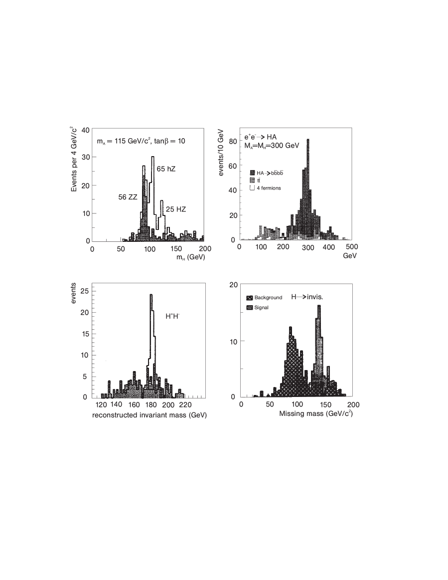
Figure 35: Experimental simulations of the search for MSSM Higgs bosons in Higgs-strahlung $hZ/HZ$, heavy pair production $HA$, charged Higgs production $H^{+}H^{-}$, and neutral invisible Higgs decays in Higgs-strahlung. Refs.[?–?].

Higgs particle of the Standard Model so that the profile of the Higgs particles can be reconstructed in supersymmetric theories.

It has been established that at least one of the Higgs particles in the SUSY spectrum could be discovered at the LHC. It has been assumed, however, in these analyses that the Higgs particles decay only into SM particles. The general consequences of decays to SUSY particles, partly invisible, have not yet been studied experimentally. A problem arises from the difficulties of establishing the heavy neutral Higgs bosons, above the top threshold, in the interesting parameter range of small to moderate $\tan\beta$. This is a problem for most of the Higgs mass estimates in supergravity inspired parametrizations. The detection of charged Higgs bosons is guaranteed, at this point, only in top decays, restricting the mass range accessible for this particle to rather low values. Thus, there are large areas in the SUSY Higgs parameter space where the ensemble of individual Higgs particles are not accessible in toto at the same time.

d) Non–Minimal Supersymmetric Extensions

The minimal supersymmetric extension of the Standard Model (MSSM) may appear very restrictive for supersymmetric theories in general, in particular in the Higgs sector where the quartic couplings are identified with the gauge couplings. However, it turns out that the mass pattern of the MSSM is quite typical if the theory is assumed to be valid up to the GUT scale – the motivation for supersymmetry per se. This general pattern has been studied thoroughly within the next-to-minimal extension: The MSSM, incorporating two Higgs isodoublets, is augmented by introducing an isosinglet field $N$. This extension leads to a model [144, 145] which is generally referred to as the (M+1)SSM.

The additional Higgs singlet can solve the so-called $\mu$–problem [i.e. to explain why $\mu={\cal O}(M_{W})$] by eliminating the $\mu$ higgsino parameter in the potential and replacing its effect by the vacuum expectation value of the $N$ field, which can be naturally related to the usual vacuum expectation values of the Higgs isodoublet fields. In this scenario the superpotential involves the two trilinear couplings $H_{1}H_{2}N$ and $N^{3}$. The consequences of this extended Higgs sector will be outlined below in the context of (s)grand unification including universal soft breaking terms of the supersymmetry [145].

The Higgs spectrum of the (M+1)SSM includes, besides the minimal set of Higgs particles, one additional scalar and pseudoscalar Higgs particle. The neutral Higgs particles are in general mixtures of the iso-scalar doublets, which couple to $W,Z$ bosons and fermions, and the iso-scalar singlet, decoupled from the non-Higgs sector. The trilinear self-interactions contribute to the masses of the Higgs particles. In contrast to the minimal model, the mass of the charged Higgs particle could be smaller than the W mass. Since the trilinear couplings increase with energy, upper bounds on the mass of the lightest neutral Higgs boson $h_{1}^{0}$ can be derived, in analogy to the Standard Model, from the assumption that the theory be valid up to the GUT scale: $m(h_{1}^{0})\stackrel{{\scriptstyle<}}{{\sim}}140$ GeV. Thus despite the additional interactions, the distinct pattern of the minimal extension remains valid also in more complex supersymmetric scenarios [146]. In fact, the mass bound of 140 GeV for the lightest Higgs particle is realized in almost all supersymmetric theories. If $h_{1}^{0}$ is (nearly) pure iso-scalar, it decouples from the gauge boson and fermion system and its rôle is taken by the next Higgs particle with a large isodoublet component, implying the validity of the mass bound again.

The couplings $R_{i}$ of the ${\cal CP}$–even neutral Higgs particles $h_{i}^{0}$ to the $Z$ boson, $ZZh_{i}^{0}$, are defined relative to the usual SM coupling. If the Higgs particle $h_{1}^{0}$ is primarily isosinglet, the coupling $R_{1}$ is small and the particle cannot be produced by Higgs-strahlung. However, in this case $h_{2}^{0}$ is generally light and couples with sufficient strength to the $Z$ boson; if not, $h_{3}^{0}$ plays this rôle. This scenario is quantified in Fig.36 where the couplings $R_{1}$ and $R_{2}$ are shown for the ensemble of allowed Higgs masses $m(h_{1}^{0})$

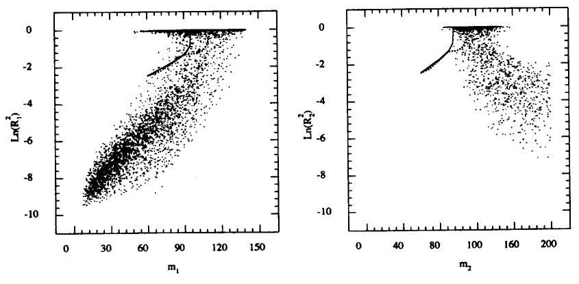
Figure 36: The couplings $ZZh_{1}$ and $ZZh_{2}$ of the two lightest $CP$–even Higgs bosons in the next-to-minimal supersymmetric extension of the Standard Model, $(M+1)SSM$. The solid lines indicate the accessible range at LEP2, the dotted lines for an energy of 205 GeV. The scatter plots are solutions for an ensemble of possible SUSY parameters defined at the scale of grand unification. Ref.[145].

and $m(h_{2}^{0})$ [adopted from Ref.[147]; see also Ref.[145, 148]]. Two different regions exist within the GUT (M+1)SSM: A densely populated region with $R_{1}\sim 1$ and $m_{1}>50$ GeV, and a tail with $R_{1}<1$ to $<<1$ and small $m_{1}$. Within this tail, the lightest Higgs boson is essentially a gauge singlet state so that it can escape detection at LEP [full/solid lines]. If the lightest Higgs boson is essentially a gauge singlet, the second lightest Higgs particle cannot be heavy. In the tail of diagram 36a the mass of the second Higgs boson $h_{2}^{0}$ varies between 80 GeV and, essentially, the general upper limit of $\sim 140$ GeV. $h_{2}^{0}$ couples with full strength to $Z$ bosons, $R_{2}\sim 1$. If in the tail of diagram 36b this coupling becomes weak, the third Higgs boson will finally take the rôle of the leading light particle.

To summarize: Experiments at $e^{+}e^{-}$ colliders are in a no-lose situation [148] for detecting the Higgs particles in general supersymmetric theories even for c.m. energies as low as $\sqrt{s}\sim 300$ GeV.

7.2 Supersymmetric Particles

The only guidelines for estimating the mass spectra of supersymmetric particles, follow from the embedding of low-energy supersymmetry into grand unified theories and the requirement of avoiding the fine tuning of parameters. The second principle is hard to quantify, yet for plausible scenarios such as those presented in Table 4, the spectra do conform to this principle. The embedding of low-energy supersymmetry into supergravity scenarios with universal soft SUSY-breaking parameters, reduces the number of free parameters, generally of order one hundred, to a few. In addition, problems of ${\cal CP}$ violation are removed etc. Given that the large ensemble of masses and mixing angles is reduced to a small number, many relations can be found among the observables which can be scrutinized with high accuracy.

It is evident from the table of masses derived for various SGUT scenarios that a large number of particles can be expected which are accessible in the first phase of the $e^{+}e^{-}$ linear colliders. In particular, the color-neutral charginos/neutralinos and sleptons, lighter than the colored squarks and gluinos, can be produced in $e^{+}e^{-}$ collisions and studied thoroughly in the clean environment of these machines. Moreover, stop particles could be light as well, partly a result of mixing effects induced by the large Yukawa coupling between L and R states in this sector. The experiments at $e^{+}e^{-}$ colliders will not only allow high-precision measurements of masses and couplings, but also of such subtle effects as mixings.

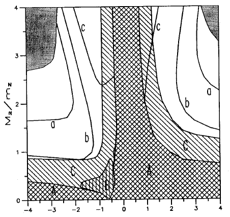
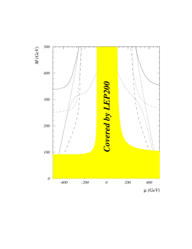
Figure 37: Left: The impact of chargino searches in the [$\mu,M_{2}$] plane of the MSSM for $\tan\beta=2$ at $\sqrt{s}=500$ GeV. The hatched region is covered by LEP2; in the grey region the chargino mass exceeds the limit of $m_{\tilde{\chi}_{1}^{\pm}}=250$ GeV. The curves a,b,c correspond to mass differences $m_{\tilde{\chi}^{\pm}_{1}}-m_{\tilde{\chi}^{0}_{1}}$ of 80, 50 and 20 GeV, respectively. Ref.[150]. Right: Supersymmetry parameter space [$\mu,M_{2}$] for neutralino production for $\tan\beta=4$ at $\sqrt{s}=500$ GeV. Shown are the limits for $e^{+}e^{-}\rightarrow\tilde{\chi}^{0}_{i}\tilde{\chi}^{0}_{j}$ in the combinations: 12 (solid); 13 (short dashes); 14 (dots); 22 (dot-dashes); 23 (long dashes). Ref.[149].

a) Charginos and Neutralinos

The ensemble of the two charginos $\tilde{\chi}_{i}^{+}$ and the four neutralinos $\tilde{\chi}_{i}^{0}$, mixtures of the [non-colored] gauginos and higgsinos, include the lightest supersymmetric particle ($LSP$) in a large part of parameter space. In the MSSM with conserved $R$–parity, the neutralino $\tilde{\chi}_{1}^{0}$ with the smallest mass is in general the lightest supersymmetric particle and stable. Only in exceptional cases sneutrinos are the lightest SUSY particles. The heavier neutralinos and the charginos decay into (possibly virtual) gauge and Higgs bosons plus the $LSP$, $\tilde{\chi}_{i}^{0}\to\tilde{\chi}_{1}^{0}+Z/W$ and $\tilde{\chi}_{1}^{0}+H$, or if they are heavy enough, into neutralino/chargino cascades, and sleptons plus leptons [149]. At the end of the cascades, the events will consist of jet pairs, leptons and $LSP$’s which escape undetected.

Neutralinos and charginos are easy to detect and to study with high accuracy at $e^{+}e^{-}$ colliders. They are produced in pairs

$$e^{+}e^{-} \to \tilde{\chi}_{i}^{+}\tilde{\chi}_{j}^{-}\hskip 42.67912pt[i,j=1,2]$$

$$e^{+}e^{-} \to \tilde{\chi}_{i}^{0}\tilde{\chi}_{j}^{0}\hskip 42.67912pt\hskip 5.69054pt[i,j=1,..,4]$$

through $s$–channel $\gamma,Z$ exchange and $t$–channel sneutrino or selectron exchange.  [Experimental details are presented in the second appendix.]  The accessible SUSY

Figure 38: Upper part: Threshold behavior of the cross section for $e^{+}e^{-}\rightarrow\tilde{\chi}^{+}_{1}\tilde{\chi}^{-}_{1}$ including initial-state radiation and beamstrahlung. Lower part: Simulation of the energy spectrum in the decay $\tilde{\chi}^{+}_{1}\rightarrow\tilde{\chi}^{0}_{1}+jj$ based on the input values $m_{\tilde{\chi}^{+}_{1}}=168.2$ GeV and $m_{\tilde{\chi}^{0}_{1}}=88.1$ GeV at $\sqrt{s}$ = 500 GeV; Ref.[151].

parameter range in the $[\mu,M_{2}]$ plane is shown in Fig.37 for the production of various chargino and neutralino pairs at 500 GeV colliders. [$\mu$ is the higgsino mass parameter while $M_{2}$ is the SU(2) gaugino mass; the U(1) gaugino mass $M_{1}$ is generally assumed to be related to $M_{2}$, with a coefficient $5/3\tan^{2}\theta_{w}$, motivated by supergravity models.] Compared to the region which can be explored by LEP2, a substantial extension can be anticipated. Since the cross sections are as large as ${\cal O}(100\ {\rm fb})$, enough events will be produced to discover these particles for masses nearly up to the kinematical limit. In fact, it has been demonstrated by detailed experimental simulations that charginos can be detected with masses up to the beam energy if the mass difference $m(\tilde{\chi}_{1}^{+})-m(\tilde{\chi}_{1}^{0})$ is sufficiently large [150].

Figure 39: Mechanisms contributing to the production of charginos in $e^{+}e^{-}$ collisions. Given are the gaugino/higgsino components that can be excited in $s$– and $t$–channel diagrams; also indicated is the impact of right-handed electron polarization.

The properties of the neutralinos and charginos can be studied in great detail at $e^{+}e^{-}$ colliders. The decay energy spectrum in $\tilde{\chi}_{1}^{+}\to\tilde{\chi}_{1}^{0}+W^{+}$ allows us to measure the mass of the $\tilde{\chi}_{1}^{+}$ particle within $\delta m_{\tilde{\chi}_{1}^{+}}=1.1$ GeV, and even better for the neutralino, c.f. Fig.38. From the fast onset $\sim\beta$ of the spin–$\frac{1}{2}$ excitation curve near the threshold, the masses can be measured very accurately. Performing a threshold scan, the error on the $\tilde{\chi}_{1}^{\pm}$ mass can be reduced to a very small value. Accuracies on the $\tilde{\chi}_{1}^{\pm}$ and $\tilde{\chi}_{1}^{0}$ masses of

$$\delta m_{\tilde{\chi}_{1}^{\pm}} \approx 100 \ {\rm MeV}$$

$$\delta m_{\tilde{\chi}_{1}^{0}} \approx 600 \ {\rm MeV}$$

can finally be achieved.

Using polarized $e^{\pm}$ beams, the decomposition of the states, $\tilde{\chi}_{1}^{-}=\alpha\tilde{W}^{-}+\beta\tilde{H}^{-}$ into Wino and higgsino components can be determined [?–?]. In general, both the Wino and higgsino components of the charginos are produced through $s$–channel $\gamma,Z$ exchange, Fig.39. However, at high energies $\gamma$ and $Z$ are demixed to $B^{0}/W^{3}$ bosons so that only the higgsino component is generated for right-handedly polarized electrons. In the second diagram, describing the $t$–channel $\tilde{\nu}_{L}$ exchange, only the Wino component couples which can be switched off/on by operating right/left polarized beams. Since the energy and angular dependence are different for the two states of L/R polarization, the mixing parameters $\alpha$ and $\beta$ can be determined directly. Similar techniques can be applied for neutralinos.

In some areas of the parameter space of supergravity models, spectacular single–$\gamma$ and $\gamma\gamma$ final states are predicted in $e^{+}e^{-}$ collisions [155]. In these models the lightest neutralino may decay into a photon $\gamma$ plus a gravitino $\tilde{G}$ which escapes undetected, or the $\tilde{\chi}^{0}_{1}\tilde{G}$ final state is produced directly:

$$e^{+}e^{-}\to \tilde{\chi}^{0}_{1}\tilde{G} \to\gamma\tilde{G}\tilde{G}\to\gamma+/E$$

$$e^{+}e^{-}\to \hskip 0.28453pt\tilde{\chi}_{1}^{0}\tilde{\chi}_{1}^{0} \to\gamma\gamma\tilde{G}\tilde{G}\to\gamma\gamma+/E$$

The most important background events to these processes are generated by the radiative return to the $Z$, $e^{+}e^{-}\rightarrow n\gamma+Z$ with the $Z$ decaying into pairs of neutrinos. This background can be eliminated by requiring the invariant missing mass, represented by $/E$, to be below the $Z$ mass. [Pure photonic events can also be generated in $e^{+}e^{-}\to\tilde{\chi}_{1}^{0}\tilde{\chi}_{2}^{0}$ and $\tilde{\chi}_{2}^{0}\tilde{\chi}_{2}^{0}$ when the branching ratio for decays $\tilde{\chi}_{2}^{0}\to\gamma\tilde{\chi}_{1}^{0}$ is non-negligible.]

b) Sleptons

The superpartners of the right-handed leptons decay into the associated SM partners and neutralinos/charginos. In major parts of the SUSY parameter space the dominant decay mode is $\tilde{\mu}_{R}\to\mu+\tilde{\chi}_{1}^{0}$ [149]. For the superpartners of the left-chiral sleptons, the decay pattern is more complicated since, besides the $\tilde{\chi}_{1}^{0}$ channels, decays into leptons and charginos can also occur. In $e^{+}e^{-}$ collisions, sleptons are produced in pairs:

$$e^{+}e^{-} \to \tilde{\mu}_{L}^{+}\tilde{\mu}_{L}^{-}\;,\;\tilde{\mu}_{R}^{+}\tilde{\mu}_{R}^{-}\;,\;\tilde{\tau}_{L}^{+}\tilde{\tau}_{L}^{-}\;,\;\tilde{\tau}_{R}^{+}\tilde{\tau}_{R}^{-}$$

$$e^{+}e^{-} \to \tilde{e}_{L}^{+}\tilde{e}_{L}^{-}\;,\;\tilde{e}_{R}^{+}\tilde{e}_{R}^{-}\;,\;\tilde{e}_{L}^{+}\tilde{e}_{R}^{-}\;,\;\tilde{e}_{R}^{+}\tilde{e}_{L}^{-}$$

$$e^{+}e^{-} \to \tilde{\nu}_{eL}\bar{\tilde{\nu}}_{eL}\;,\;\tilde{\nu}_{\mu L}\bar{\tilde{\nu}}_{\mu L}\;,\;\tilde{\nu}_{\tau L}\bar{\tilde{\nu}}_{\tau L}$$

For charged sleptons, the production proceeds via $\gamma,Z$ exchange in the $s$–channel. In the case of selectrons, additional $t$–channel neutralino exchange is present, which is also responsible for the production of the mixed left and right-chiral selectron states. For sneutrinos, the production process is mediated by $s$–channel $Z$–exchange and, in the case of electron-sneutrinos, by $t$–channel exchange of charginos in addition.

The cross sections for the pair production of sleptons are of the order of 5 to 15 fb ,c.f. Fig.40 (upper part), so that their discovery is very easy up to the kinematical limit [156]. Enough events will be produced to study their detailed properties. From the sharp threshold behavior of the excitation curve and/or decay spectra the masses

Figure 40: Upper part: The cross section of the production of $\tilde{\mu}\tilde{\mu}$ pairs in $e^{+}e^{-}$ collisions for different electron-beam polarizations. Lower part: Decay lepton energy spectrum in $\tilde{\mu}_{R}\to\mu\tilde{\chi}^{0}_{1}$ for $m_{\tilde{\mu}_{R}}$ = 275.1 GeV and $m_{\tilde{\chi}^{0}_{1}}$ = 88.1 GeV at the energy $\sqrt{s}$ = 800 GeV; also shown is the background from $WW$ pair production. Ref.[151].

of the $\tilde{\mu}$ and $\tilde{\chi}_{1}^{0}$ can be determined [151] up to a level of

$$\delta m_{\tilde{\mu}}=1.8\hskip 5.69054pt{\rm GeV}$$

c.f. Fig.40 (lower part). By analysing the angular distribution in the production process, the spin of the sleptons can be checked to be zero. The polarization of the $e^{\pm}$ beams will help to identify the couplings of these particles.

The opportunity to analyze the $\tau$ helicity [157] in the decay $\tilde{\tau}_{L}^{-}\to\tau_{\lambda}^{-}\tilde{\chi}_{1}^{0}$ ($\lambda=$ L/R) can be exploited to discriminate between the gaugino and higgsino components of $\tilde{\chi}_{1}^{0}$. The gaugino component of $\tilde{\chi}_{1}^{0}$, coupled in a chirality-conserving vertex, gives rise to left-handed $\tau_{L}^{-}$ states, the higgsino component, coupled in a chirality-flip vertex, to right-handed $\tau_{R}^{-}$ states. The analysis can readily be extended to the more complicated scenario of L/R mixed $\tilde{\tau}$ states.

Selectrons can be produced in association with gauginos in $e\gamma$ collisions: $e\gamma\to\tilde{e}\tilde{\chi}_{1}^{0}\to e\tilde{\chi}_{1}^{0}\tilde{\chi}_{1}^{0}$ etc. For small $\tilde{\chi}_{1}^{0}$ masses, the kinematic range of the selectron mass extends beyond the $e^{\pm}$ beam energy [158]. However, it seems difficult to exploit this window in practice, since for masses beyond the $e^{\pm}$ beam energies the rates are quite low.

c) Stop particles

The stop particles $\tilde{t}_{1}$ may have small masses [159] compared to the other squarks for two reasons. First, due to the large Yukawa terms, the mass term of the top squark may evolve to much lower values than the mass terms for first and second generation squarks [see e.g. Ref.[136]]. Second, mixing due to large Yukawa terms between $\tilde{t}_{L}$ and $\tilde{t}_{R}$ leads to a large splitting of the mass values associated with the mass eigenstates $\tilde{t}_{1}$ and $\tilde{t}_{2}$. Stop experiments can therefore be exploited to measure the soft SUSY-breaking trilinear scalar coupling $A$. [Similar phenomena may also be observed in the $\tilde{b}$ and $\tilde{\tau}$ sectors, less pronounced though [160].] In $e^{+}e^{-}$ collisions the following final states can be generated [160]

$$e^{+}e^{-}\to\tilde{t}_{1}\bar{\tilde{t}}_{1},\tilde{t}_{2}\bar{\tilde{t}}_{2}\;\;\hskip 5.69054pt{\rm and}\;\;\hskip 5.69054pt\tilde{t}_{1}\bar{\tilde{t}}_{2}\;+\;c.c$$

either by $\gamma,Z$ exchange for diagonal or $Z$ exchange for mixed final states. The production rates are determined by the masses and the mixing angle $\Theta_{\tilde{t}}$ [161]. Depending on the mass ratios, stop particles can decay into many final states. For heavy states, $\tilde{t}_{2}$ in particular [162]: $\tilde{t}_{i}\to t\tilde{\chi}_{j}^{0},b\tilde{\chi}_{j}^{+},t\tilde{g}$ or $\tilde{t}_{i}\to\tilde{b}W^{+},\tilde{b}H^{+}$, among which the first two modes are in general dominant.

Depending on the masses and energies, the production cross sections are generally in the range between 10 and 100 fb so that the search can be performed very efficiently and the properties of the particles can be determined in detail.  Using polarized $e^{-}$

Figure 41: The measurement of the light stop mass $m_{\tilde{t}_{1}}$ and the mixing angle $\Theta_{\tilde{t}}$ of the stop sector in $e^{+}e^{-}\rightarrow\tilde{t}_{1}\overline{\tilde{t}}_{1}$ for 90% left– and right-handedly polarized electron beams at $\sqrt{s}$ = 500 GeV. The central values correspond to $m_{\tilde{t}_{1}}$ = 180 GeV and $|\cos\Theta_{\tilde{t}}|=0.57$. Ref.[160].

beams, both the $\tilde{t}_{1}$ mass and the mixing angle $\Theta_{\tilde{t}}$ can be measured in diagonal pair production $e^{+}e^{-}\to\tilde{t}_{1}\bar{\tilde{t}_{1}}$ of the lightest stop state. A study of this reaction has been performed at $\sqrt{s}=500$ GeV, $m_{\tilde{t}_{1}}=180$ GeV for the left-right stop mixing angle $|\cos\Theta_{\tilde{t}}|=0.57$ which corresponds to the minimum of the cross section [160]. The cross sections at tree level for these parameters are $\sigma_{L}=48.6$ fb and $\sigma_{R}=46.1$ fb for 90% left– and right-polarized $e^{-}$ beams, respectively. Based on detailed simulations, the experimental errors on these cross sections are estimated to be $\Delta\sigma_{L}=\pm 6$ fb and $\Delta\sigma_{R}=\pm 4.9$ fb. Figure 41 shows the resulting error bands and the corresponding error ellipse in the $[m_{\tilde{t}_{1}},\cos\Theta_{\tilde{t}}]$ plane. The experimental accuracy for the $\tilde{t}_{1}$ mass and the stop mixing angle are $m_{\tilde{t}_{1}}=180\pm 7$ GeV and $|\cos\Theta_{\tilde{t}}|=0.57\pm 0.06$.

The sbottom system can be treated analogously. If $\tan\beta$ is moderate, mixing effects can be neglected. Taking $m_{\tilde{b}_{1}}=200$ GeV, $m_{\tilde{b}_{2}}=220$ GeV, the cross sections and the expected experimental errors are $\sigma_{L}(e^{+}e^{-}\to\tilde{b}_{1}\bar{\tilde{b}}_{1})=61.1\pm 6.4$ fb, $\sigma_{R}(e^{+}e^{-}\to\tilde{b}_{2}\bar{\tilde{b}}_{2})=6\pm 2.6$ fb for 90% left– and right-polarized $e^{-}$ beams. The resulting experimental errors are $m_{\tilde{b}_{1}}=200\pm 4$ GeV, $m_{\tilde{b}_{2}}=220\pm 10$ GeV. With these results, the mass of the heavier stop particle can be predicted: $m_{\tilde{t}_{2}}=289\pm 15$ GeV.

This prediction allows us to fix the MSSM parameters in a subtle domain. Assuming that $\mu$ and $\tan\beta$ are known from other neutralino/chargino experiments [e.g. $\mu=-200$ GeV and $\tan\beta=2$], the soft breaking parameters of the stop and sbottom systems can be derived: $m_{\tilde{Q}}=195\pm 4$ GeV, $m_{\tilde{U}}=138\pm 26$ GeV, $m_{\tilde{D}}=219\pm 10$ GeV, $A_{t}=-236\pm 38$ GeV if $\cos\Theta_{\tilde{t}}>0$, and $A_{t}=36\pm 38$ GeV if $\cos\Theta_{\tilde{t}}<0$.

d) SUSY at LC and LHC: La Cohabitation

Since the mass scale of low-energy supersymmetry is restricted to order 1 TeV, the LHC will either find signals of supersymmetry or rule out low-energy supersymmetry. In this collider, squarks and gluinos can be detected with masses up to about 1.5 to 2 TeV [14]. $e^{+}e^{-}$ linear colliders can provide the necessary complementary information in the sector of non-colored supersymmetric particles.

The analysis of supersymmetric particles at the LHC can be divided into two categories. First, the gross features of supersymmetric phenomena, such as missing transverse energy, dileptons etc., will be measured. These measurements will allow us to determine the typical mass scale of colored supersymmetric particles. Second, if in specific scenarios cascade decays with favorable branching ratios can be exploited, a remarkably high precision can be reached in determining mass differences between supersymmetric particles at the LHC [14]. For example, from the analysis of the decay chain $\tilde{g}\to\tilde{b}\to\tilde{\chi}_{2}^{0}\to\tilde{\chi}_{1}^{0}$ in “LHC Point 3” of the study Ref.[14], the mass difference $m(\tilde{\chi}_{2}^{0})-m(\tilde{\chi}_{1}^{0})$ can be measured within $\pm 50$ MeV, and $m(\tilde{g})-m(\tilde{b})$ within 2 GeV accuracy. In a similar way, the masses of other squarks can be determined within a few percent. The corresponding observation and high-precision analyses of the heavier charginos and neutralinos have not yet been demonstrated. The situation in the scalar slepton sector is similar. If the rates are large enough to generate signals of sleptons, their properties can be determined in some points of the SUSY parameter space. Assuming that the soft SUSY-breaking parameters are universal, the entire set of the basic parameters can be generated at the LHC with an accuracy at the percent level.

This experimental scenario at the LHC is easy to compare with the scenario at $e^{+}e^{-}$ colliders. While the discovery limits at the LHC can be extended to values above 1 TeV, the experiments at the $e^{+}e^{-}$ machines provide high-precision information on all the supersymmetric particles which are kinematically accessible, in the high energy range for masses up to $\sim$1 TeV. In particular, the analysis of the color-neutral states, charginos/neutralinos and sleptons which are generally (much) lighter than the colored states, can be carried out with high accuracy, independently of specific assumptions and solely based on kinematics. Masses, for instance, can be measured by exploiting threshold effects or simple decay kinematics. Even such subtle properties as the mixing of states can be analyzed thoroughly in polarization experiments. Thus, a systematic and high-precision study can be performed which will resolve the complexities of the supersymmetric phenomena. In this way, the complete supersymmetry scenario can be reconstructed up to the kinematical limit in a comprehensive form and the structure of the underlying microscopic theory can be uncovered.

7.3 Testing SUSY–GUT

The high precision with which masses, couplings and mixing parameters will be determined at $e^{+}e^{-}$ colliders, can be exploited to test the structure of the underlying theories [153]. If minimal supergravity is the fundamental theory, the observable properties of the superparticles can be expressed by a small set of parameters defined at the GUT scale. As a result, many relations can be found among the masses of the superparticles and other observables which can stringently be tested at $e^{+}e^{-}$ colliders.

An overconstrained set of observables can be collected, slepton and gaugino/neutralino masses and production cross sections, for instance, which can be expressed by five basic parameters, as shown for a few examples in Table 5, c.f. Refs. [?–?].

Masses :	$m(\tilde{l}_{L})$	$\Leftarrow$	$m_{0}$		$M_{1\!/\!2}$		$\tan\beta$
	$m(\tilde{l}_{R})$	$\Leftarrow$	$m_{0}$		$M_{1\!/\!2}$		$\tan\beta$
	$m(\tilde{\chi}_{1}^{\pm})$	$\Leftarrow$			$M_{2}$	$\mu$	$\tan\beta$
	$m(\tilde{\chi}_{1,2}^{0})$	$\Leftarrow$		$M_{1}$	$M_{2}$	$\mu$	$\tan\beta$
Cross Sections :	$\sigma(e_{L}^{-}e^{+}\to\tilde{e}_{L}^{-}\tilde{e}_{L}^{+})$	$\Leftarrow$	$m_{0}$	$M_{1}$	$M_{2}$	$\mu$	$\tan\beta$
	$\sigma(e_{R}^{-}e^{+}\to\tilde{e}_{R}^{-}\tilde{e}_{R}^{+})$	$\Leftarrow$	$m_{0}$	$M_{1}$	$M_{2}$	$\mu$	$\tan\beta$
	$\sigma(e_{L}^{-}e^{+}\to\tilde{\chi}_{1}^{-}\tilde{\chi}_{1}^{+})$	$\Leftarrow$	$m_{0}$		$M_{2}$	$\mu$	$\tan\beta$
	$\sigma(e_{R}^{-}e^{+}\to\tilde{\chi}_{1}^{-}\tilde{\chi}_{1}^{+})$	$\Leftarrow$			$M_{2}$	$\mu$	$\tan\beta$

Table 5: The dependence of a representative set of observables on the underlying SUSY and SUGRA parameters. [The parameters are defined below.]

Two characteristic examples [153] should illustrate the great potential of $e^{+}e^{-}$ colliders in this context:

$(i)$ The gaugino masses at the scale of $\rm SU(2)\times U(1)$ symmetry breaking are related to the common gaugino mass $M_{1\!/\!2}$ at the GUT scale by the running gauge couplings:

$$M_{i}=\frac{\alpha_{i}}{\alpha_{\rm GUT}}M_{1\!/\!2}\hskip 22.76219pt[\;i=1,2,3\;{\rm for\;U(1),SU(2),SU(3)}\;]$$ (22)

with $\alpha_{\rm GUT}$ being the gauge coupling at the unification scale. The mass relation in the non-color sector

$$\frac{M_{1}}{M_{2}}=\frac{5}{3}\tan^{2}\theta_{W}\approx\frac{1}{2}$$ (23)

can be tested stringently to $\sim 0.5$ % by measuring the masses and production cross sections of charginos/neutralinos and sleptons as shown in Fig.42 (upper part).

$(ii)$ In a similar way the slepton masses can be expressed in terms of the common scalar mass parameter $m_{0}$ at the GUT scale, contributions $\sim M_{1\!/\!2}^{2}$ due to the evolution from the GUT scale down to low energies, and the D terms related to the electroweak symmetry breaking. The masses of the charged R/L sleptons and the sneutrino can be written as

$$m^{2}(\tilde{l}_{R}) = m_{0}^{2}+\kappa_{R}M_{1\!/\!2}^{2}-\sin^{2}\theta_{w}\cos 2\beta\,M_{Z}^{2}$$

$$m^{2}(\tilde{l}_{L}) = m_{0}^{2}+\kappa_{L}M_{1\!/\!2}^{2}-{\textstyle\frac{1}{2}}(1-2\sin^{2}\theta_{W})\cos 2\beta\,M_{Z}^{2}$$

$$m^{2}(\tilde{\nu}_{L}) = m_{0}^{2}+\kappa_{L}M_{1\!/\!2}^{2}+{\textstyle\frac{1}{2}}\cos 2\beta\,M_{Z}^{2}$$ (24)

with $\kappa_{R}=0.15$ and $\kappa_{L}=0.52$ determined by the solution of the evolution equations. These expressions give rise to simple relations among slepton masses after eliminating the common scalar mass parameter:

$$m^{2}(\tilde{l}_{L})-m^{2}(\tilde{\nu_{L}}) = -\cos^{2}\theta_{w}\cos 2\beta\,M_{Z}^{2}$$

$$m^{2}(\tilde{l}_{L})-m^{2}(\tilde{l}_{R}) = (\kappa_{L}-\kappa_{R})M_{1\!/\!2}^{2}-{\textstyle\frac{1}{2}}(1-4\sin^{2}\theta_{W})\cos 2\beta\,M_{Z}^{2}$$ (25)

The second relation follows from assuming the universality of the scalar masses, in particular $m_{0}({\bf 5^{*}})=m_{0}({\bf 10})$ within $\rm SU(5)$. This assumption can be tested by relating the mass difference between $\tilde{e}_{L}$ and $\tilde{e}_{R}$ to the $\rm SU(2)$ gaugino mass $M_{1\!/\!2}$, as shown in Fig.42 (lower part).

7.4 Supersymmetry with R–Parity Violation

The most general gauge and supersymmetry invariant Lagrangian with minimal particle content admits also the following Yukawa interactions [163]

$$W=\lambda_{ijk}L_{i}L_{j}\overline{E}_{k}+\lambda_{ijk}^{\prime}L_{i}Q_{j}\overline{D}_{k}+\lambda_{ijk}^{\prime\prime}\overline{U}_{i}\overline{D}_{j}\overline{D}_{k}$$ (26)

where $L$, $Q$ are the left-handed lepton and quark superfields while $\overline{E}$, $\overline{D}$, $\overline{U}$ are the corresponding right-handed fields. If both lepton-number violating ($\lambda_{ijk}$ and $\lambda_{ijk}^{\prime}$) and baryon-number violating ($\lambda_{ijk}^{\prime\prime}$) couplings were present, they would give rise to very fast proton decay. In the MSSM all terms in Eq.(26) are eliminated by imposing a multiplicative symmetry, $R$–parity: all SM particles are assigned $R=+1$, their superpartners have $R=-1$ [164]. However, since the $R$–parity has no a priori justification,

Figure 42: Testing mass relations at $e^{+}e^{-}$ colliders between gauginos, and between selectrons (lower part), as predicted in minimal supergravity; Refs.[152, 153].

the possibilities of having either $\Delta L\neq 0$ or $\Delta B\neq 0$ (but not both) should be investigated as well. If $R$–parity is broken, the model differs from the MSSM in two important features:

a) The lightest SUSY particle (LSP) is not protected any more, and it can decay into conventional particles. As a result, the signature of missing energy for MSSM processes disappears.

b) Supersymmetric particles can be produced singly in collisions of conventional particles, thus extending the mass range that can be probed for a given energy.

To illustrate a typical case, the production of a single superparticle in $e^{+}e^{-}$ collisions may be outlined, Fig.43, arising from the lepton-number violating term $\lambda_{LLE}L_{e}L_{i}\overline{E_{e}}$, $i=\mu$, $\tau$ [165],

$$e^{+}e^{-}\rightarrow\tilde{\nu_{i}}\rightarrow l_{i}^{\pm}\tilde{\chi}_{k}^{\mp},\ \nu_{i}\tilde{\chi}_{k}^{0}$$

with the subsequent decays

$$\tilde{\chi}_{1}^{-} \rightarrow \tilde{\chi}_{1}^{0}l^{-}\nu,\ e^{-}l_{i}^{-}e^{+},\ or\ e^{-}\nu_{e}\nu_{i}$$

$$\tilde{\chi}_{1}^{0} \rightarrow e^{\pm}l_{i}^{\mp}\nu_{e},\ e^{\pm}e^{\mp}\nu_{i}$$

The large number of charged leptons in the final state can be exploited as a characteristic signature in this scenario. These events should be clearly visible at $e^{+}e^{-}$

Figure 43: Typical behavior of cross sections for $R$–parity breaking supersymmetry in the lepton sector; Ref.[165].

colliders provided the couplings $\lambda_{i}$ are sufficiently large. For example, at $\sqrt{s}=500$ GeV single chargino production with $m_{\chi^{+}}=400$ GeV should be observed for $\lambda_{LLE}=0.01$ and a sneutrino mass in the range of 300 to 600 GeV. Depending on the couplings $\lambda_{LLE}$, $\tilde{\nu}$ decays to lepton pairs [166]

$$e^{+}e^{-}\rightarrow\tilde{\nu_{i}}\rightarrow e^{+}e^{-},\mu^{+}\mu^{-},\tau^{+}\tau^{-}$$

provide signatures that are very easy to detect experimentally.

If the $LQ\bar{D}$ interaction term is non-zero, leptoquark-like phenomena are predicted to occur. This case will be discussed in detail in the following section.

8 The Alternative: Compositeness

In supersymmetric extensions of the Standard Model, the fundamental particles are pointlike down to distances close to the Planck length. However, if light Higgs particles do not exist, the electroweak bosons become strongly interacting at energies of order 1 TeV. As one among other physical scenarios, this could be interpreted as a signal of composite substructures of these particles at a scale of $10^{-17}$ cm. Moreover, the proliferation of quarks and leptons could be taken as evidence for possible substructures of the matter particles [167]. In this picture, masses and mixing angles are a consequence of the interactions between a small number of elementary constituents – in perfect analogy to the quark/gluon picture of hadrons. No theoretical formalism has been set up so far which would reconcile, in a satisfactory manner, the small masses in the Standard Model with the tiny radii of these particles which imply very large kinetic energies of these constituents. However, the lack of theoretical formalism does not invalidate the physical picture or its motivation.

8.1 Bounds on the Electron Radius

In this agnostic approach, stringent bounds have been derived from high energy scattering experiments on possible non-zero radii of leptons, quarks and gauge bosons from $Z$ decay data [168] and Bhabha scattering [169] in $e^{+}e^{-}$ collisions, as well as from electron-quark and quark-quark scattering at HERA [170] and the Tevatron [171], respectively. From these analyses the compositeness scale has been bounded to less than $10^{-17}$ cm.

Møller scattering $e^{-}e^{-}\to e^{-}e^{-}$ at high energies provides a very powerful instrument to set limits on electron compositeness. This problem has been studied in Ref.[172], based on four-electron contact interactions which can be generated by the exchange of electron constituents [173]:

$${\cal L}_{C}=\frac{2\pi}{\Lambda_{c}^{2}}\bar{e}_{L}\gamma_{\mu}e_{L}\cdot\bar{e}_{L}\gamma_{\mu}e_{L}$$ (27)

The strength of the interaction has been set to $g_{*}^{2}/4\pi=1$. The (inverse) contact scale $\Lambda_{c}$ can be identified, within an uncertainty of a factor of order 3, with the radius of the electron. Detailed experimental simulations have shown that Møller scattering is superior to Bhabha scattering in this context, a simple consequence of the bigger cross section in the central rapidity region. The high polarization that can be achieved for electron beams, gives Møller scattering another advantage. At c.m. energies of 1 TeV, the bound on electron compositeness can be set to

$$\Lambda_{c}\approx 150\;\;{\rm TeV}\hskip 8.53581pt\Rightarrow R_{e}\stackrel{{\scriptstyle<}}{{\sim}}\hskip 8.53581pt10^{-18}{\rm cm}$$

for an integrated luminosity of $\int{\cal{L}}\sim$ $100$ fb^-1 if polarized electrons are used, Fig.44. These high-energy electron-electron scattering experiments will provide us with direct and unambiguous limits on the radius of the electron. This is in contrast to high-precision $(g-2)_{e}$ and $(g-2)_{\mu}$ measurements, the interpretation of which depends on dynamical assumptions on the underlying constituent theory.

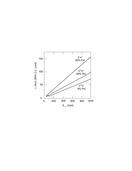
Figure 44: Bounds on the compositeness scale of electrons, extracted from large angle Møller scattering $e^{-}e^{-}\to e^{-}e^{-}$. At $\sqrt{s}=1$ TeV the integrated luminosity is assumed to be $\int{\cal{L}}$ $=80{\rm fb}^{-1}$; Ref.[172].

8.2 Excited States

In compositeness pictures, excited states should be observed with masses of order of the compositeness scale $\Lambda_{c}$, i.e. $m_{*}\sim 1$ TeV. Such states can be produced pairwise and singly, generated by the exchange of constituents [174]: $e^{+}e^{-}\to e_{*}^{+}e_{*}^{-}$ and $e^{+}e^{-}\to e^{+}e_{*}^{-}$ etc. Since the constituent exchange interactions are strong, the masses of the excited states which can be probed, extend up to the kinematical limit $m(e_{*})\sim\sqrt{s}$ for single $e_{*}$ production. The decay modes of the excited states, besides magnetic dipole decays to gauge bosons $e^{*}\to e\gamma,eZ$ and $\nu W$, are contact decays $e^{*}\to e+l\bar{l}$ and $e+jj$ with branching ratios of similar size.

8.3 Leptoquarks

A very exciting prediction of fermion compositeness is the existence of leptoquarks [175]. They are novel bound states of subconstituents which build up leptons and quarks in this scenario. While the size of the couplings to $\gamma$ and $Z$ bosons follows from the electroweak symmetries, the Yukawa couplings to leptons and quarks are bound by experiment. In the interesting mass range, these Yukawa couplings are expected to be weak.

These particles can also occur in grand unified theories. Moreover, in supersymmetric theories in which the $R$ parity is broken, scalar particles, squarks or sleptons, may be coupled to quarks and leptons, giving rise to production mechanisms and decay signatures analogous to leptoquarks [176]. However, whereas leptoquarks per se disintegrate solely to leptons and quarks, a wide variety of decay modes is in general expected for squarks and sleptons, including the large ensemble of standard supersymmetric decay channels, see e.g. [177]. Since leptoquark bound states in the compositeness picture build up a tower of states with non-zero spins, the phenomenology of the two scenarios is clearly distinct.

Leptoquarks can exist in a large variety of states carrying $[l_{i}q_{j}]$ or $[l_{i}\overline{q}_{j}]$ quantum numbers $(i,j=L,R)$ and being scalar or vectorial in the simplest representations [178], see Table 6. They can be produced in $e^{+}e^{-}$ collisions pairwise,

$$e^{+}e^{-}\to LQ+\overline{LQ}$$

through $s$–channel $\gamma,Z$ exchange and partly through $t$–channel $q$ exchange [179, 180]. The cross sections for the production of scalar leptoquarks scale asymptotically as $\log(s/M_{LQ}^{2})/s$. The cross sections for vector leptoquarks approach non-zero limits for $s$–channel $\gamma,Z$ exchange, or they grow with $s$ due to the $t$–channel $q$ exchange until the rise is damped by form factors [180]. The typical size of the cross sections is illustrated in Fig. 45.

Type ${}^{Q}\overline{LQ}_{T}$ Decay $\sigma_{tot}(s)[$fb$]$ ${}^{-1/3}S_{0}$ $\displaystyle\begin{array}[]{c}e_{L}^{-}u_{L}\\ e_{R}^{-}u_{R}\\ \nu_{e}d_{L}\end{array}$ $6~{}$ ${}^{-4/3}\tilde{S}_{0}$ $e_{R}^{-}d_{R}$ $98~{}$ ${}^{+2/3}S_{1}$ $\nu_{e}u_{L}$ $110~{}$ ${}^{-1/3}S_{1}$ $\displaystyle\begin{array}[]{c}\nu_{e}d_{L}\\ e_{L}^{-}u_{L}\end{array}$ $6~{}$ ${}^{-4/3}S_{1}$ $e_{L}^{-}d_{L}$ $158~{}$ $\displaystyle\begin{array}[]{c}{}^{-2/3}S_{1/2}\\ \\ {}^{-5/3}S_{1/2}\end{array}$ $\displaystyle\begin{array}[]{c}\nu_{e}\bar{u}_{L}\\ e_{R}^{-}\bar{d}_{R}\\ e_{L}^{-}\bar{u}_{L}\\ e_{R}^{-}\bar{u}_{R}\end{array}$ $\displaystyle\begin{array}[]{r}65\\ \\ 149\end{array}$ $\displaystyle\begin{array}[]{c}{}^{+1/3}\tilde{S}_{1/2}\\ {}^{-2/3}\tilde{S}_{1/2}\end{array}$ $\displaystyle\begin{array}[]{c}\nu_{e}\bar{d}_{L}\\ e_{L}^{-}\bar{d}_{L}\end{array}$ $\displaystyle\begin{array}[]{r}27\\ 39\end{array}$ Type ${}^{Q}\overline{LQ}_{T}$ Decay $\sigma_{tot}(s)[$fb$]$ $\displaystyle\begin{array}[]{c}{}^{-1/3}V_{1/2}\\ \\ {}^{-4/3}V_{1/2}\end{array}$ $\displaystyle\begin{array}[]{c}\nu_{e}d_{R}\\ e_{R}^{-}u_{L}\\ e_{L}^{-}d_{R}\\ e_{R}^{-}d_{L}\end{array}$ $\displaystyle\begin{array}[]{r}365\\ \\ 895\end{array}$ $\displaystyle\begin{array}[]{c}{}^{+2/3}\tilde{V}_{1/2}\\ {}^{-1/3}\tilde{V}_{1/2}\end{array}$ $\displaystyle\begin{array}[]{c}\nu_{e}u_{R}\\ e_{L}^{-}u_{R}\end{array}$ $\displaystyle\begin{array}[]{r}353\\ 247\end{array}$ $e_{L}^{-}\bar{d}_{R}$ ${}^{-2/3}V_{0}$ $e_{R}^{-}\bar{d}_{L}$ $222~{}$ $\nu_{e}\bar{u}_{R}$ ${}^{-5/3}\tilde{V}_{0}$ $e_{R}^{-}\bar{u}_{L}$ $1370~{}$ ${}^{+1/3}V_{1}$ $\nu_{e}\bar{d}_{R}$ $942~{}$ ${}^{-2/3}V_{1}$ $\displaystyle\begin{array}[]{c}e_{L}^{-}\bar{d}_{R}\\ \nu_{e}\bar{u}_{R}\end{array}$ $222~{}$ ${}^{-5/3}V_{1}$ $e_{L}^{-}\bar{u}_{R}$ $1790~{}$

Table 6: The total cross section $\sigma_{tot}(s)$ are given for $\sqrt{s}=500$GeV and a leptoquark mass $M_{LQ}=200$GeV, assuming vanishing Yukawa couplings; corrections due to beamstrahlung and initial state radiation are included. Ref.[181].

Figure 45: Total cross section for leptoquark pair production at fixed center-of-mass energy as a function of the leptoquark mass $M_{LQ}$ assuming vanishing Yukawa couplings; corrections due to beamstrahlung and ISR are included. Ref.[181].

$+{\textstyle\frac{1}{3}}$ $+{\textstyle\frac{2}{3}}$

The particles decay to a charged lepton, or a neutrino, and a jet, giving rise to visible (a) $l^{+}l^{-}jj$, (b) $l^{\pm}jj$, and (c) $jj$ final states. Since leptoquarks generate a peak in the invariant ($lj$) mass, they are easy to detect in the cases (a) and (b) up to mass values close to the kinematical limit [181]: The discovery range extends up to $m_{LQ}\stackrel{{\scriptstyle<}}{{\sim}}(0.37-0.49)\sqrt{s}$ for scalar leptoquarks, and up to $m_{LQ}\stackrel{{\scriptstyle<}}{{\sim}}(0.48-0.5)\sqrt{s}$ for vector leptoquarks.

Since leptoquarks carry color, they are produced copiously [182] in hadron collisions through the subprocesses $gg,q\bar{q},qq\to LQ+LQ^{\prime}$ and $gq\to LQ+l$. Leptoquarks can therefore be generated at the LHC with very high masses. Experiments at $e^{+}e^{-}$ colliders are nevertheless important to identify the electroweak properties of these novel states.

Bibliography

- [1] S.L. Glashow, Nucl. Phys. 20 (1961) 579; S. Weinberg, Phys. Rev. Lett. 19 (1967) 1264; A. Salam, in Elementary Particle Theory, ed. N. Svartholm (Almqvist and Wiksells, Stockholm 1968).
- [2] H. Fritzsch and M. Gell-Mann, Proc. XVI Int. Conf. on High Energy Physics, eds. J.D. Jackson and A. Roberts (Fermilab 1972).
- [3] P.W. Higgs, Phys. Rev. Lett. 12 (1964) 132; Phys. Rev. 145 (1966) 1156; F. Englert and R. Brout, Phys. Rev. Lett. 13 (1964) 321; G.S. Guralnik, C.R. Hagen and T.W. Kibble, Phys. Rev. Lett. 13 (1964) 585.
- [4] H. Georgi and S. Glashow, Phys. Rev. Lett. 32 (1974) 438.
- [5] J. Wess and B. Zumino, Nucl. Phys. B70 (1974) 39.
- [6] J.C. Pati and A. Salam, Phys. Rev. D10 (1974) 275.
- [7] The physics program of linear colliders is summarized in: P.M. Zerwas, Proc. of Les Rencontres de la Vallée d’Aoste, La Thuile 1994, ed. M. Greco (Editions Frontières); H. Murayama and M.E. Peskin, Ann. Rev. Nucl. and Part. Science 46 (1997) 533.
- [8] For detailed analyses see: Proceedings, Physics and Experiments with Linear Colliders, Saariselkä 1991, eds. R. Orava, P. Eerola and M. Nordberg (World Scientific 1992); Proceedings, Physics and Experiments with Linear Colliders, Waikoloa/Hawaii 1993, eds. F. Harris, S. Olsen, S. Pakvasa and X. Tata (World Scientific 1993); Proceedings, Physics and Experiments with Linear Colliders, Morioka 1995, eds. A. Miyamoto, Y. Fujii, T. Matsui and S. Iwata (World Scientific 1996).
- [9] Much of the material described in this report had been worked out in a series of workshops: Proceedings, Collisions at 500 GeV: The Physics Potential, Munich–Annecy–Hamburg 1991/93, DESY 92-123A+B, 93-123C; Proceedings, Collisions at TeV Energies: The Physics Potential, Annecy–Gran Sasso–Hamburg 1995, DESY 96-123D, ed. P.M. Zerwas.
- [10] Proceedings of the Electron-Electron Linear Collider Workshop, Santa Cruz 1995, ed. C.A. Heusch [Int. J. of Mod. Phys. 11 (1996) 1523].
- [11] Proceedings of the Workshop on Gamma-Gamma Colliders, Berkeley 1994 [Nucl. Instr. Meth. A355 (1995) 19].
- [12] ATLAS Technical Proposal, CERN/LHCC/94-43; CMS Technical Proposal, CERN/LHCC /94-38.
- [13] DPF Study, Electroweak Symmetry Breaking and Beyond the Standard Model, eds. T. Barklow, S. Dawson, H.E. Haber and S. Siegrist (World Scientific 1996); DPF/DBP Summer Study on New Directions for High-Energy Physics, Snowmass 1996.
- [14] Workshop on Supersymmetry at LHC, LHCC Meeting, org. J. Ellis (CERN 1996).
- [15] P.A. Baikov et al., Proceedings of the X. Workshop on High Energy Physics and Quantum Field Theory (QFTHEP-96), Moscow 1996, ed. B. Levtchenko, V. Sarin; E.E. Boos, M.N. Dubinin, V.A. Ilyin, A.E. Pukhov and V.I. Savrin, SNUTP-94-116, Korean Physical Society meeting, 1994.
- [16] I.F. Ginzburg, G.L. Kotkin, S.L. Panfil, V.G. Serbo and V.I. Telnov, Nucl. Instr. Meth. 219 (1984) 5.
- [17] J.H. Kühn, E. Mirkes and J. Steegborn, Z. Phys. C57 (1993) 615.
- [18] M. Kobayashi and T. Maskawa, Prog. Theor. Phys. (Kyoto) 49 (1973) 652.
- [19] D. Schaile and P.M. Zerwas, Phys. Rev. D45 (1992) 3262.
- [20] M. Veltman, Nucl. Phys. B123 (1977) 89.
- [21] D. Schaile, Proc. XXVII Intern. Conf. on High Energy Physics, Glasgow 1994, eds. P.J. Bussey and I.G. Knowles (Inst. Phys. Publ.).
- [22] F. Abe et al. [CDF Coll.], Phys. Rev. D50 (1994) 2966 and Phys. Rev. Lett. 74 (1995) 2626; S. Abachi et al. [D0 Coll.], Phys. Rev. Lett. 74 (1995) 2632.
- [23] I. Bigi, Yu. Dokshitzer, V. Khoze, J. Kühn and P.M. Zerwas, Phys. Lett. 181B (1986) 157.
- [24] M. Jezabek and J.H. Kühn, Nucl. Phys. B314 (1989) 1;
- [25] H. Murayama and Y. Sumino, Phys. Rev. D47 (1993) 82; K. Fujii, T. Matsui and Y. Sumino, Phys. Rev. D50 (1994) 4341; P. Comas et al., in Part D of Ref.[9]; D. Schulte et al., in: DESY–ECFA Conceptual LC Design Report (1997).
- [26] O. Podobrin, see P. Igo-Kemenes in Waikoloa Proceedings of Ref.[8].
- [27] F.M. Borzumati and N. Polonsky, in Part D of Ref.[9].
- [28] A. Venturi in Part C of Ref.[9]; P. Igo-Kemenes, Waikoloa Proceedings of Ref.[8].
- [29] G. Blair, A. Juste, M. Martinez, D. Schulte, C.H. Shepherd-Themistocleous, in: DESY–ECFA Conceptual LC Design Report (1997).
- [30] J. Jersak, E. Laermann and P.M. Zerwas, Phys. Rev. D25 (1982) 1218.
- [31] A. Djouadi and M. Spira in Part B of Ref.[9]; G.L. Kane, G.A. Ladinsky and C.P. Yuan, Phys. Rev. D45 (1992) 124.
- [32] T. Barklow and C. Schmidt, Proceedings, 1994 DPF Meeting, Albuquerque (World Scientific).
- [33] R. Harlander, M. Jezabek, J.H. Kühn and M. Peter, Z. Phys. C73 (1997) 477.
- [34] M.E. Peskin and M. Schmidt in Saariselkä Proceedings of Ref.[8].
- [35] W. Bernreuther et al. in Part D of Ref.[9].
- [36] V.S. Fadin and V.A. Khoze, JETP Lett. 46 (1987) 525; Sov. J. Nucl. Phys. 48 (1988) 309.
- [37] M.J. Strassler and M.E. Peskin, Phys. Rev. D43 (1991) 1500.
- [38] M. Jezabek, J.H. Kühn and T. Teubner, Z. Phys. C56 (1992) 653; Y. Sumino, K. Fujii, K. Hagiwara, M. Murayama and C.K. Ng, Phys. Rev. D47 (1992) 56.
- [39] M. Jezabek and J.H. Kühn, Phys. Lett. B316 (1993) 360.
- [40] P. Igo-Kemenes, M. Martinez, R. Miquel and S. Orteu in Part C of Ref.[9]; P. Comas, R. Miquel, M. Martinez and S. Orteu in Part D of Ref.[9].
- [41] M. Veltman, Acta Phys. Polon. B8 (1977) 475.
- [42] F. Jegerlehner, private communication; see S. Eidelman and F. Jegerlehner, Z. Phys. C67 (1995) 585.
- [43] D. Gross and F. Wilczek, Phys. Rev. Lett. 30 (1973) 1343; H.D. Politzer, Phys. Rev. Lett. 30 (1973) 1346.
- [44] S. Bethke, Proceedings of the QCD Euroconference 96, PITHA 96/30, (Montpellier), and private communication.
- [45] P. Aurenche et al. in part D of Ref.[9].
- [46] C.F. von Weizsäcker, Z. Phys. 88 (1934) 612; E.J. Williams, Phys. Rev. 45 (1934) 729.
- [47] T. Barklow, P. Chen and W. Kozanecki in Part B of Ref.[9]; D. Schulte, in: DESY–ECFA Conceptual LC Design Report (1997).
- [48] T.F. Walsh and P.M. Zerwas, Phys. Lett. B44 (1973) 195; E. Witten, Nucl. Phys. B120 (1977) 189; W.A. Bardeen and A.J. Buras, Phys. Rev. D20 (1979) 166.
- [49] G. Schuler and T. Sjöstrand, Nucl. Phys. B407 (1993) 539.
- [50] R. Engel et al. in part D of Ref.[9]; A. Corsetti, R.M. Godbole and G. Pancheri, in part D of Ref.[9].
- [51] I.F. Ginzburg, in part D of Ref.[9].
- [52] D.J. Miller and A. Vogt in part D of Ref.[9].
- [53] C. Peterson, T.F. Walsh and P.M. Zerwas, Nucl. Phys. B174 (1980) 424.
- [54] T. Kleinwort and G. Kramer, Nucl. Phys. B477 (1996) 3.
- [55] S.J. Brodsky, T.A. DeGrand, J.F. Gunion and J.H. Weis, Phys. Rev. Lett. 41 (1978) 672; C.H. Llewellyn Smith, Phys. Lett. B79 (1978) 83.
- [56] J. Binnewies, B.A. Kniehl and G. Kramer, Phys. Rev. D53 (1996) 6110.
- [57] M. Drees, M. Krämer, J. Zunft and P.M. Zerwas, Phys. Lett. B306 (1993) 371; M. Cacciari et al., Nucl. Phys. B466 (1996) 173; M. Cacciari et al. in part D of Ref.[9].
- [58] M. Drees and R.M. Godbole, J. Phys. G21 (1995) 1559.
- [59] E. Laenen, S. Riemersma, J. Smith and W.L. van Neerven, Phys. Rev. D49 (1994) 5753.
- [60] E.A. Kuraev, L.N. Lipatov and V.S. Fadin, Sov. Phys. JETP 45 (1977) 199; I.I. Balitski and L.N. Lipatov, Sov. J. Nucl. Phys. 28 (1978) 822.
- [61] J. Bartels, A. De Roeck and H. Lotter, DESY 96-168; S.J. Brodsky, F. Hautmann and D.E. Soper, SLAC-PUB-7218.
- [62] C.H. Llewellyn Smith, Phys. Lett. B46 (1973) 233.
- [63] W. Alles, C. Boyer and A. Buras, Nucl. Phys. B119 (1977) 125.
- [64] W. Beenakker et al. in Part A of Ref.[9].
- [65] V. Barger, K. Cheung, T. Han and R.J.N. Phillips, Phys. Rev. D52 (1995) 3815.
- [66] W. Kilian, Report DESY 96-187; E. Boos, H.-J. He, A. Pukhov, W. Kilian, C.P. Yuan, and P.M. Zerwas, DESY 96-256.
- [67] M. Peskin in Saariselkä Proceedings of Ref.[8].
- [68] R. Casalbuoni, P. Chiappetta, A. Deandrea, S. DeCurtis, D. Dominici, and R. Gatto, in Part C of Ref.[9].
- [69] Communication by M. Swartz and G. Wilson.
- [70] H. Nowak et al., in: DESY–ECFA Conceptual LC Design Report (1997).
- [71] A. Blondel, in: Polarization at LEP, eds. G. Alexander et al., CERN 88-06.
- [72] K. Flöttmann, DESY 95-064 and private communication.
- [73] K.J.F. Gaemers and G.J. Gounaris, Z. Phys. C1 (1979) 259; K. Hagiwara, K. Hikasa, R.D. Peccei and D. Zeppenfeld, Nucl. Phys. B282 (1987) 253.
- [74] K. Mönig, in Part D of Ref.[9].
- [75] G. Gounaris and C.G. Papadopoulos, DEMO-HEP-96/04.
- [76] S.Y. Choi and F. Schrempp, Phys. Lett. B272 (1991) 149.
- [77] D. Choudhury and J. Kalinowski, Nucl. Phys. 491 (1997) 129.
- [78] W. Buchmüller and D. Wyler, Nucl. Phys. B268 (1986) 621.
- [79] K. Hagiwara, S. Ishihara, R. Szalapski and D. Zeppenfeld, Phys. Lett. B283 (1992) 353, and Phys. Rev. D48 (1993) 2182.
- [80] M. Kuroda, F.M. Renard, and D. Schildknecht, Phys. Lett. B183 (1987) 366.
- [81] D. Dashalakis, A. Kyriakis, C. Markou, E. Simopoulou, H. Nowak, R. Shanidze and I. Riu, in: DESY–ECFA Conceptual LC Design Report (1997).
- [82] T. Appelquist and C. Bernard, Phys. Rev. D22 (1980) 200; A. Longhitano, Nucl. Phys. B188 (1981) 118; A. Falk, M. Luke and E.H. Simmons, Nucl. Phys. B365 (1991) 523; F. Boudjema, in Part C of Ref.[9].
- [83] A. Nippe and T. Ohl, in: DESY–ECFA Conceptual LC Design Report (1997).
- [84] G. Bélanger and F. Boudjema, Phys. Lett. B288 (1992) 201.
- [85] G. Bélanger and F. Boudjema, Phys. Lett. B288 (1992) 210.
- [86] L. Okun, Leptons and Quarks (North Holland Pub. Comp. 1982).
- [87] T. Barklow, Proceedings of the Snowmass Workshop 1996.
- [88] R. Casalbuoni, S. DeCurtis, D. Dominici and R. Gatto, Phys. Lett. B155 (1985) 95.
- [89] A. Djouadi, in Morioka Proceedings of Ref.[8].
- [90] A. Djouadi, A. Leike, T. Riemann, D. Schaile and C. Verzegnassi, Z. Phys. C56 (1992) 289.
- [91] A. Leike and S. Riemann, in Part D of Ref.[9].
- [92] V. Barger et al., Phys. Rev. D33 (1986) 1912; T.G. Rizzo, Phys. Rev. D34 (1986) 1438; F. del Aguila, E. Laermann and P.M. Zerwas, Nucl. Phys. B297 (1988) 1; W. Buchmüller and C. Greub, Nucl. Phys. B363 (1991) 345; F. Csikor, A. Djouadi and I. Montvay, in Part B of Ref.[9].
- [93] J. Maalampi, J. Pietilä and J. Vuori, Phys, Lett. B297 (1992) 327; P. Minkowski, Int. J. Mod. Phys. A11 (1996) 1591; C.A. Heusch and P. Minkowski, ibid. 1607; T. Rizzo, Int. J. Mod. Phys. A11 (1996) 1613.
- [94] J.F. Gunion, Int. J. Mod. Phys. A11 (1996) 1551.
- [95] G. Barenboim, K. Huitu, J. Maalampi and M. Raidal, Phys. Lett. B394 (1997) 132.
- [96] N. Cabibbo, L. Maiani, G. Parisi and R. Petronzio, Nucl. Phys. B158 (1979) 295; M. Sher, Phys. Rep. 179 (1989) 273; M. Lindner, Z. Phys. C31 (1986) 295; G. Altarelli and G. Isidori, Phys. Lett. B337 (1994) 141; J. Casas, J. Espinosa and M. Quiros, Phys. Lett. B342 (1995) 171.
- [97] T. Hambye and K. Riesselmann, DO-TH-96-20 and private communication.
- [98] A. Hasenfratz, T. Neuhaus, K. Jansen, H. Yoneyama and C.B. Lang, Phys. Lett. B199 (1987) 531; M. Lüscher and P. Weisz, Phys. Lett. B212 (1988) 472; M. Göckeler, H. Kastrup, T. Neuhaus and F. Zimmermann, Nucl. Phys. B404 (1993) 517.
- [99] LEP Electroweak Working Group, R. Clare et al., CERN-PPE/96-183; A. Blondel, Proceedings of the XXVIII Intern. Conf. on High Energy Physics, Warsaw 1996.
- [100] J. Ellis, M.K. Gaillard and D.V. Nanopoulos, Nucl. Phys. B106 (1976) 292; B.L. Ioffe and V.A. Khoze, Sov. J. Part. Nucl. 9 (1978) 50; B.W. Lee, C. Quigg and H.B. Thacker, Phys. Rev. D16 (1977) 1519.
- [101] V. Barger, K. Cheung, A. Djouadi, B.A. Kniehl and P. Zerwas, Phys. Rev. D49 (1994) 79.
- [102] D.R.T. Jones and S.T. Petcov, Phys. Lett. B84 (1979) 440.
- [103] R.N. Cahn and S. Dawson, Phys. Lett. B136 (1984) 96; G.L. Kane, W.W. Repko and W.B. Rolnick, Phys.. Lett. B148 (1984) 367.
- [104] G. Altarelli, B. Mele and F. Pitolli, Nucl. Phys. B287 (1987) 205; W. Kilian, M. Krämer and P.M. Zerwas, Phys. Lett. B373 (1996) 135.
- [105] G.J. Gounaris, F. Renard and D. Schildknecht, Phys. Lett. B83 (1979) 191; V. Barger, T. Han and R.J.N. Phillips, Phys. Rev. D38 (1988) 2766; V. Barger and T. Han, Mod. Phys. Lett. A5 (1990) 667; F. Boudjema and E. Chopin, ENSLAPP-A-534-95.
- [106] A. Djouadi, M. Spira and P.M. Zerwas, Z. Phys. C70 (1996) 427.
- [107] E. Boos, M. Sachwitz, H.J. Schreiber and S. Shichanin, Z. Phys. C61 (1994) 675.
- [108] P. Grosse-Wiesmann, D. Haidt and H.J. Schreiber, in Part A of Ref.[9].
- [109] H.J Schreiber et al., in: DESY–ECFA Conceptual LC Design Report (1997).
- [110] D.L. Borden, D.A. Bauer, and D.O. Caldwell, Phys. Rev. D48 (1993) 4018.
- [111] G.V. Jikia, Phys. Lett. B298 (1993) 224; Nucl. Phys. B405 (1993) 24.
- [112] O.J.P. Eboli, M.C. Gonzales-Garcia, F. Halzen, and D. Zeppenfeld, Phys. Rev. D48 (1993) 1430; M. Baillargeon, G. Belanger, and F. Boudjema, Phys. Rev. D51 (1995) 4712.
- [113] K. Hagiwara, I. Watanabe, and P.M. Zerwas, Phys. Lett. B278 (1992) 187; E. Gabrielli, V.A. Ilyin and B. Mele, ROME1-1165/97 (NDU-HEP-97-EG01).
- [114] P. Janot, in Waikoloa Proceedings of Ref.[8].
- [115] M. Hildreth, T. Barklow and D. Burke, Phys. Rev. D49 (1994) 3441; possible improvements on BR() are discussed in M. Battaglia et al., in: DESY–ECFA LC Conceptual LC Design Report (1997).
- [116] M. Battaglia and R. Vuopionperä, in: DESY–ECFA Conceptual LC Design Report (1997).
- [117] A. Djouadi, J. Kalinowski and P.M. Zerwas, Mod. Phys. Lett. A7 (1992) 1765 and Z. Phys. C54 (1992) 255.
- [118] K. Hagiwara, H. Murayama and I. Watanabe, Nucl. Phys. B367 (1991) 257.
- [119] E. Witten, Nucl. Phys. B188 (1981) 513; J. Polchinski and L. Susskind, Phys. Rev. D26 (1982) 3661; S. Dimopoulos and H. Georgi, Nucl. Phys. B193 (1981) 150; N. Sakai, Z. Phys. C11 (1981) 153.
- [120] K. Inoue, A. Kakuto, H. Komatsu and S. Takeshita, Progr. Theor. Phys. 68 (1982) 927, (E) 70 (1983) 330, 71 (1984) 413; L.E. Ibañez and G.G. Ross, Phys. Lett. B110 (1982) 215; L. Alvarez-Gaumé, M. Claudson and M.B. Wise, Nucl. Phys. B207 (1982) 96; J. Ellis, D.V. Nanopoulos, and K. Tamvakis, Phys. Lett. B121 (1983) 123; M. Drees, Phys. Rev. D38 (1988) 718.
- [121] J.-P. Derendinger, L.E. Ibanez and H.P. Nilles, Phys. Lett. B155 (1985) 65; M. Dine, R. Rohm, N. Seiberg and E. Witten, Phys. Lett. B156 (1985) 55.
- [122] P. Fayet and S. Ferrara, Phys. Rep. 32 (1977) 249; H.P. Nilles, Phys. Rep. 110 (1984) 1; H.E. Haber and G.L. Kane, Phys. Rep. 117 (1985) 75.
- [123] L.E. Ibañez and G.G. Ross, Phys. Lett. B105 (1981) 439; S. Dimopoulos, S. Raby and F. Wilczek, Phys. Rev. D24 (1981) 1681.
- [124] J. Ellis, S. Kelley and D.V. Nanapoulos, Phys. Lett. B249 (1990) 441; P. Langacker and M. Luo, Phys. Rev. D44 (1991) 817; U. Amaldi, W. de Boer and H. Fürstenau, Phys. Lett. B260 (1991) 447; P. Langacker, in: Precision Tests of the Standard Electroweak Model (World Scientific 1995).
- [125] V. Barger, M.S. Berger and P. Ohmann, Phys. Rev. D49(1993) 4908.
- [126] H. Baer and M. Brhlik, FSU-HEP-960801.
- [127] H. Baer, M. Brhlik and R. Munroe, Phys. Rev. D52 (1995) 5031.
- [128] M. Drees and S. Martin, in: Electroweak Symmetry Breaking and Beyond the Standard Model, eds. T. Barklow, S. Dawson, H. Haber and J. Siegrist (World Scientific).
- [129] S. Mrenna, ANL-HEP-PR-96-63.
- [130] K. Inonue, A. Kakuto, H. Komatsu and S. Takeshita, Progr. Theor. Phys. 67 (1982) 1889; R. Flores and M. Sher, Ann. Phys. 148 (1983) 95; H.P. Nilles and M. Nusbaumer, Phys. Lett. B145 (1984) 73; P. Majumdar and P. Roy, Phys. Rev. D30 (1984) 2432.
- [131] J.F. Gunion and H.E. Haber, Nucl. Phys. B272 (1986) 1 and B278 (1986) 449.
- [132] Y. Okada, M. Yamaguchi and T. Yanagida, Progr. Theor. Phys. 85 (1991) 1; H. Haber and R. Hempfling, Phys. Rev. Lett. 66 (1991) 1815; J. Ellis, G. Ridolfi and F. Zwirner, Phys. Lett. 257B (1991) 83; M. Carena, J.R. Espinosa, M. Quiros and C.E.M. Wagner, Phys. Lett. B335 (1995) 209; H.E. Haber, R. Hempfling and A. Hoang, CERN-TH-95-216 and Z. Phys. C in press.
- [133] H.E. Haber, in: Conference on Beyond the Standard Model IV, Lake Tahoe 1994, ed. J.F. Gunion et al. (World Scientific).
- [134] A. Djouadi, J. Kalinowski and P.M. Zerwas, Z. Phys. C70 (1996) 435.
- [135] A. Djouadi, P. Janot, J. Kalinowski and P.M. Zerwas, Phys. Lett. B376 (1996) 220.
- [136] A. Djouadi, J. Kalinowski, P. Ohmann and P.M. Zerwas, DESY 95-213 and Z. Phys. C 74 (1997) 93.
- [137] A. Bartl, H. Eberl, K. Hidaka, T. Kon, W. Majerotto and Y. Yamada, Phys. Lett. B389 (1996) 538.
- [138] A. Djouadi, J. Kalinowski and P.M. Zerwas, Z. Phys. C57 (1993) 569.
- [139] M. Krämer, J. Kühn, M.L. Stong and P.M. Zerwas, Z. Phys. C64 (1994) 21.
- [140] A. Djouadi, H.E. Haber and P.M. Zerwas, Phys. Lett. B375 (1996) 203.
- [141] P. Janot, in Waikoloa Proceedings of Ref.[8].
- [142] A. Andreazza and C. Troncon, in: DESY–ECFA Conceptual LC Design Report (1997).
- [143] A. Sopczak, Z. Phys. C65 (1995) 449.
- [144] P. Fayet, Nucl. Phys. B90 (1975) 104; H.-P. Nilles, M. Srednicki and D. Wyler, Phys. Lett. B120 (1983) 346; J.-P. Derendinger and C.A. Savoy, Nucl. Phys. B237 (1984) 307; J..F. Gunion and H.E. Haber, Nucl. Phys. B272 (1986) 1; J. Ellis, J.F. Gunion, H.E. Haber, L. Roszkowski and F. Zwirner, Phys. Rev. D39 (1989) 844.
- [145] U. Ellwanger, M. Rausch de Traubenberg and C.A. Savoy, Z. Phys. C67 (1995) 665; S.F. King and P.L. White, Phys. Rev. D52 (1995) 4183; H. Asatrian and K. Eguin, Mod. Phys. Lett. A10 (1995) 2943.
- [146] J.R. Espinosa and M. Quiros, Phys. Lett. B279 (1992) 92; G.L. Kane, C. Kolda and J.D. Wells, Phys. Rev. Lett. 70 (1993) 2686.
- [147] M. Carena, P.M. Zerwas [conv.] et al., Proceedings, Physics at LEP2, eds. G. Altarelli, T. Sjöstrand and F. Zwirner, CERN 96-01.
- [148] J. Kamoshita, Y. Okada and M. Tanaka, Phys. Lett. B328 (1994) 67.
- [149] A. Bartl, W. Majerotto and B. Mösslacher in Part B of Ref.[9].
- [150] J.-F. Grivaz in Part B of Ref.[9].
- [151] U. Martyn, in: DESY–ECFA Conceptual LC Design Report (1997).
- [152] S. Orito in Waikoloa Proceedings of Ref.[8].
- [153] T. Tsukamoto, K. Fujii, H. Murayama, M. Yamaguchi and Y. Okada, Phys. Rev. D51 (1995) 3153.
- [154] J.L. Feng, M.E. Peskin, H. Murayama and X. Tata, Phys. Rev. D52 (1995) 1418.
- [155] J. Ellis, K. Enqvist and D. Nanopoulos, Phys. Lett. B147 (1984) 99; S. Dimopoulos, M. Dine, S. Raby, and S. Thomas, Phys. Rev. Lett. 76 (1996) 3494; S. Ambrosiano, G. Kane, G. Kribs, S. Martin and S. Mrenna, Phys. Rev. Lett. 76 (1996) 3498; D.R. Stump, M. Wiest, and C.P. Yuan, Phys. Rev. D54 (1996) 1936; J.L. Lopez, D.V. Nanopoulos and A. Zichichi, CTP-TAMU-45/96.
- [156] R. Becker, R. Starosta and C. Van der Velde in Part B and Part C of Ref.[9].
- [157] M.M. Nojiri, Phys. Rev. D51 (1995) 6281.
- [158] D. Borden, D. Bauer and D. Caldwell, SLAC-PUB-5715 (1992); H. König and K. Peterson, Phys. Lett. B294 (1992) 110; F. Cuypers, G. van Oldenborgh and R. Rückl, Nucl. Phys. B383 (1992) 45.
- [159] J. Ellis and S. Rudaz, Phys. Lett. B128 (1983) 248.
- [160] A. Bartl, H. Eberl, S. Kraml, W. Majerotto, W. Porod and A. Sopczak in Part D of Ref.[9].
- [161] K. Hikasa and M. Kobayashi, Phys. Rev. D36 (1987) 724.
- [162] S. Kraml, H. Eberl, A. Bartl, W. Majerotto and W. Porod, Phys. Lett. B386 (1996) 175; A. Djouadi, W. Hollik and C. Jünger, KA-TP-20-96; W. Beenakker, R. Höpker, T. Plehn and P.M. Zerwas, DESY 96-178 and Z. Phys. C in press.
- [163] L.J. Hall and M. Suzuki, Nucl. Phys. B231 (1984) 419.
- [164] L.E. Ibañez and G.G. Ross, Phys. Lett. B260 (1991) 291.
- [165] H. Dreiner and S.Lola, in part D of Ref.[9].
- [166] J. Kalinowski, R. Rückl, H. Spiesberger and P.M. Zerwas, Report DESY 97–044.
- [167] H. Harari, Proceedings, 1984 Scott. Summer School (St. Andrews); M.E. Peskin, Proceedings, Int. Symp. on Lepton and Photon Interactions at High Energies, eds. M. Konuma and K. Takahashi, (Kyoto 1985); W. Buchmüller, Acta Phys. Austr. Suppl. XXVII (1985) 517.
- [168] G. Köpp, D. Schaile, M. Spira and P.M. Zerwas, Z. Phys. C 65 (1995) 545.
- [169] H. Kroha, Phys. Rev. D46 (1992) 58; G. Alexander et al., CERN-PPE 96-098.
- [170] S. Aid et al., Phys. Lett. B353 (1995) 578.
- [171] F. Abe et al., Phys. Rev. Lett. 75 (1995) 608.
- [172] T.L. Barklow, Int. J. Mod. Phys. A11 (1996) 1579.
- [173] E. Eichten, K.D. Lane and M.E. Peskin, Phys. Rev. Lett. 50 (1983) 811.
- [174] R. Kleiss and P.M. Zerwas, Proceedings, Physics at Future Accelerators, ed. J.H. Mulvey (La Thuile and Geneva 1987), CERN 87-07.
- [175] See e.g. J.L. Hewett and T.G. Rizzo, Phys. Rep. 183 (1989) 193.
- [176] H. Dreiner, in part B of Ref.[9].
- [177] E. Perez, Y. Sirois, and H. Dreiner, Proceedings, Future Physics at HERA, eds. G. Ingelman, H. DeRoeck, and R. Klanner, DESY 1996.
- [178] W. Buchmüller, R. Rückl and D. Wyler, Phys. Lett. B191 (1987) 442.
- [179] D. Schaile and P.M. Zerwas, Proceedings, Physics at Future Accelerators, ed. J.H. Mulvey (La Thuile and Geneva 1987), CERN 87-07; A. Djouadi, M. Spira and P.M. Zerwas in Part B of Ref.[9].
- [180] J. Blümlein and R. Rückl, Phys. Lett. B304 (1993) 337; J. Blümlein and E. Boos, Nucl. Phys. B (Proc. Suppl.) 37 (1994) 181; J. Blümlein, E. Boos, and A. Kryukov, DESY 96-219 and Phys. Lett. B in press.
- [181] R. Rückl, R. Settles, and H. Spiesberger, in: DESY–ECFA Conceptual LC Design Report (1997).
- [182] J. Hewett and S. Pakvasa, Phys. Rev. D37 (1988) 3165; O.J.P. Éboli and A.V. Olinto, Phys. Rev. D38 (1988) 3461; J. Blümlein, E. Boos, and A. Kryukov, DESY 96-174 and Z. Phys. C in press.