Abstract

We present a new three-dimensional Monte-Carlo code MUSIC (MUon SImulation Code) for muon propagation through the rock. All processes of muon interaction with matter with high energy loss (including the knock-on electron production) are treated as stochastic processes. The angular deviation and lateral displacement of muons due to multiple scattering, as well as bremsstrahlung, pair production and inelastic scattering are taken into account. The code has been applied to obtain the energy distribution and angular and lateral deviations of single muons at different depths underground. The muon multiplicity distributions obtained with MUSIC and CORSIKA (Extensive Air Shower simulation code) are also presented. We discuss the systematic uncertainties of the results due to different muon bremsstrahlung cross-sections.

PACS number(s): 94.40T
Keywords: High energy muons, Muons underground, Monte Carlo methods, Interaction of particles with matter.

1 Introduction

Muon transport through the rock plays an important role in ’underground physics’, in particular in the underground cosmic-ray experiments. The muon ’depth-intensity curve’ related to the muon energy spectrum at sea level and to the primary cosmic-ray specrum, muon multiplicity distribution and ’decoherence curve’ related to the mass composition of primaries and to the characteristics of high-energy hadron-nucleus interactions are influenced by the muon propagation through the rock. The large underground detectors designed to search for rare events (such as proton decay, neutrino interactions etc.) are not free from the background of cosmic-ray muons and muon-produced secondary particles. The propagation of muons produced by high-energy astrophysical and atmosheric neutrinos in the rock should be also taken into account. These examples show the importance of an accurate three-dimensional simulations of the muon transport in matter.

There are several three-dimensional codes for the simulation of muon propagation through the rock (see, for example, [1, 2, 3]). They have been used to obtain the characteristics of muon flux and muon bundles deep underground and to describe the experimental data. However, the increase of the accuracy of the recent and future measurements requests an adequate increase of the accuracy of the calculations. The accuracy of the calculations is restricted by the uncertainties in the cross-sections and the assumptions made to simplify the computational procedure (due to the restricted CPU time). Recently, a new corrections to the muon bremsstrahlung and knock-on electron production cross-sections were calculated [4]. A new generation of powerful computers allows to avoid many simplifications in the calculation procedure.

In our code, named MUSIC (MUon SImulation Code) we have used the most recent and accurate cross-sections of the muon interactions with matter and we tried to avoid many simplifications used in the previous simulations. This three-dimensional code is based on an algorithm of a one-dimensional muon propagation code described in [5] and used to fit the ’depth-intensity relation’ measured by LVD [6, 7]. We have treated all processes of muon interaction with high energy transfer (bremsstrahlung, inelastic scattering, pair production and knock-on electron production) as the stochastic ones if the fraction of energy lost by muon is more than $10^{-3}$. The mean muon path between two interactions with the energy loss more than $10^{-3}$ is about 20 hg/cm². The angular deviation of muons was taken into account not only in the process of multiple scattering (as it was usually done) but also in the processes of bremsstrahlung, inelastic scattering and pair production. We investigated the effect due to the last three processes.

We have performed three-dimensional simulations of the muon transport through Gran Sasso and standard rocks. The results of such simulations for Gran Sasso rock, as well as the complete description of the code and related topics can be found in [8]. Here we present the results of the calculations for standard rock using two different bremsstrahlung cross-sections [4, 9]. In this way we investigated the effect due to the uncertainties in the cross-sections. We have also applied the code to calculate muon multiplicity distribution using CORSIKA [10] code for the simulations of Extensive Air Showers.

The main features of the MUSIC code are described in Section 2. The results of the simulation in the standard rock are presented in Section 3. We also discuss in Section 3 the dependence of our results on the cross-sections and assumptions used in the code. The results of the full Monte-Carlo simulation of muon component using CORSIKA and MUSIC can be found in Section 4. In Section 5 we present our conclusions.

2 The code

In the code we have treated energy losses due to ionization, bremsstrahlung, pair production and muon – nucleus inelastic scattering.

The mean energy loss is usually expressed by

$$-<\frac{dE}{dx}>=\alpha(E)+\beta(E)E\$$ (1)

where $\alpha$ is the energy loss due to ionization and $\beta$ is the relative energy loss due to other processes.

Ionization can be considered as a continuous process and it is well described by Bethe-Bloch formula. On the contrary, in other processes a particle can lose a big fraction of its energy in a single interaction and it is necessary to treat these kinds of energy losses in two separate parts, one continuous and the other stochastic. To improve the simulation procedure and to study the importance of the stochasticity of the knock-on electron production we have divided the energy loss due to this process into two parts: continuous loss with $v<v_{cut}=10^{-3}$ which we calculate using the Bethe-Bloch formula, and stochastic loss which we treat in the same way as other stochastic processes. Thus, the energy losses due to knock-on electron production, bremsstrahlung, pair production and inelastic scattering are expressed by:

$$<\frac{dE}{dx}> = <\frac{dE}{dx}>_{cont}+<\frac{dE}{dx}>_{stoc}$$ (2)

$$= E\frac{N}{A}\int_{0}^{v_{cut}}dvv\frac{d\sigma}{dv}+E\frac{N}{A}\int_{v_{cut}}^{1}dvv\frac{d\sigma}{dv}\$$

where A is the mass number of the material, N is the Avogadro number, $v$ is the fraction of the transferred muon energy and $\frac{d\sigma}{dv}$ is the cross-section of the process.

The differential probability that a muon loses a fraction $v$ of its energy per g/cm² in a stochastic way is given by

$$\frac{dP}{dv}=\frac{N}{A}\frac{d\sigma}{dv}$$ (3)

It is quite difficult to choose a suitable value for $v_{cut}$, because a little value of $v_{cut}$, that means an accurate simulation, results in an increase of CPU’s time. We have chosen $v_{cut}=10^{-3}$ that seems meet all requirements. On a DEC AlphaStation 250 4/266 the simulation of 10 TeV muons propagated through 3 km.w.e. takes 0.02 s/muon.

We note that most of the other codes use higher value of $v<v_{cut}$ and/or are considering the knock-on electron production as a continuous process.

The aim of the code is to propagate a muon through a layer X of standard rock (we used A=22, Z=11, $\rho$= 2.65 g/cm³). If we know the initial energy of the particle $E_{0}$ , its starting point $x_{0},\ y_{0},z_{0}$ in the rock and its direction $\theta_{0},\ \phi_{0}$, we can simulate with an iterative procedure, step by step,  muon interaction point according to $P(|\overrightarrow{r}|)=\frac{1}{\lambda}e^{-|\overrightarrow{r}|/\lambda(\sigma)}$, where $\overrightarrow{r}$ is the vector which defines the interaction point in the space and $\lambda$ is the mean free path. Then the continuous and stochastic energy losses, as well as lateral and angular displacement due to multiple Coulomb scattering are evaluated. Moreover the code simulates the angular deviations caused by the stochastic processes.

Finally we check if the muon has crossed the layer X, and in this case we store its final energy $E_{f}$ , its direction $\theta_{f},\ \phi_{f}$ and the coordinates of its arrival point $x_{f},\ y_{f},z_{f}$.

To describe pair production we have used the cross-section given by Kokoulin-Petrukhin [11]. The code samples separately muon energy loss and angular deflection. The second one is sampled following the parametrization proposed in [12] (see Appendix A).

Two different muon bremsstrahlung cross-sections, one given by Bezrukov and Bugaev [9] and the other recently proposed by Kelner, Kokoulin and Petrukhin [4] are available in MUSIC. These two calculations differ mainly by the account of bremsstrahlung on atomic electrons, when the photon is emitted by the target electron.

The code samples the fraction of muon energy transferred to the photon and separately the muon scattering angle, following also in this case the parametrisation proposed by [12] (see Appendix A).

We carried out additional test of the simulation of muon deflection angle due to pair production and bremsstrahlung process using a simplified procedure based on the GEANT parametrizations [13, 14]. We concluded that this approach leads to a little underestimation of the muon deflection due to these processes with respect to Van Ginneken’s parametrizations.

Among stochastic processes, the angular deflection due to inelastic scattering on nuclei is expected to be dominant [15]. In this case to calculate the muon energy loss and angular deflection we have used double-differential cross section $\frac{d^{2}\sigma}{dvdQ^{2}}$ obtained by Bezrukov and Bugaev [16], where Q is the four-momentum transferred. We have sampled the muon scattering angle $\theta_{\mu}$ according to the aforementioned cross-section using the relation $Q^{2}=2(E_{\mu 0}E_{\mu f}-P_{\mu 0}P_{\mu f}cos\theta_{\mu}-m_{\mu}^{2})$. Since the muon inelastic scattering is expected to be the most important for angular deviation of muons (with the exception of multiple scattering), this process has been treated in a more correct way (using the double-differential cross-section) in comparison with other stochastic processes. However, the cross-section of this process proposed in [16] is valid only at low $Q^{2}$ (the accuracy is not worse than $11\%$ for $Q^{2}\leq 3$ GeV² and energy transfers from 1 to 10⁶ GeV [16]).

Some authors [12, 17, 18], pointed out the complexity of the problem to sample simultaneously the emission angle of the photon, the deflection angle of the muon and the fractional energy loss $v$. The accurate and simultaneous simulation of the angles and energies can be important for muons exceeding 1 TeV, where the deflection due to bremsstrahlung could be dominant [12]. As it will be discussed in the next section, however, even if we used the same approach as in [12], we didn’t find such behaviour, and the multiple scattering appears to be the dominant mechanism of deflection of muons passing through the large thickness of matter. A complete treatment of these aspects is currently beyond the aim of our code.

We have treated multiple Coulomb scattering in the Gaussian approximation [20]. We have considered the projections of muon angular deviation, $\theta_{\mu}$, and lateral displacement, $l$, on two orthogonal planes which include the initial direction of muon. The projections of angular deviation and lateral displacement of muon with respect to its initial direction at each step between two interactions with $v>v_{cut}$ are distributed according to correlated Gaussians with mean values and dispersions calculated using the formulae:

$$<\theta_{x}>=<\theta_{y}>=0,\ \ \ \sigma_{\theta}^{2}=<\theta_{x}^{2}>=<\theta_{y}^{2}>=\frac{\epsilon_{ms}^{2}}{2\lambda}\int_{0}^{x}\frac{dx}{E_{\mu}^{2}}\$$ (4)

$$<l_{x}>=<l_{y}>=0\ \ \ \sigma_{l}^{2}=<l_{x}^{2}>=<l_{y}^{2}>=\frac{\epsilon_{ms}^{2}}{6\lambda\rho^{2}}\int_{0}^{x}\frac{dxx^{2}}{E_{\mu}^{2}}\$$ (5)

where $\epsilon_{ms}$ = 21.2 MeV, $\lambda$ = 26.48 g/cm² is the radiation length in standard rock and $\rho$ = 2.65 $g/cm^{3}$ is the standard rock density. As discussed in the next section, we have checked also if the use of a more accurate treatment of multiple scattering (e.g. Molière theory) leads to different results.

3 Results

We have propagated 100000 muons through 3 km.w.e. and 1000000 through 10 km. w.e. with MUSIC using Kelner-Kokoulin-Petrukhin’s cross-section for bremsstrahlung. Initial muon energy has been sampled according to a primary energy spectrum with index $\gamma=3.7$. In the case of 3 km.w.e. minimal muon energy $E_{0}$ was fixed to 900 GeV, while for 10 km.w.e. $E_{0}$ was 9 TeV, corresponding in each case to a survival probability of less or about 0.3%.

Figures 1, 2 and 3 show energy, lateral and angular distributions at 3 and 10 km.w.e. The mean muon energy is 250 GeV at 3 km.w.e. and 367 GeV at 10 km.w.e. This result is in agreement with the simple consideration that the mean muon energy at a depth $h$ increases with $h$.

Mean angular deviation $<\alpha>$ is 0.56^∘ at 3 km.w.e. and 0.45^∘ at 10 km.w.e. Angular deviation is mainly caused by multiple Coulomb scattering. This process produces a deviation that increases when energy decreases. This explains why at 3 km.w.e., when $<E_{h}>$ is lower, $<\alpha>$ is higher than at 10 km.w.e.

Figures 4 and 5 show lateral and angular distributions obtained with MUSIC and PROPMU – a code for muon propagation in rock written by P. Lipari and T. Stanev [2]. The codes are completely independent, but their results are practically the same. This fact confirms the correctness of both simulations and shows that the effects of angular deviations due to stochastic processes, with the approximations discussed in previous section, are really very little, 1-2 orders of magnitude less than the effects due to multiple scattering. In fact, as Lipari and Stanev treat only angular deviation due to multiple scattering, and in MUSIC all possible angular deviations are taken into account, the distributions obtained with these two codes do not show any appreciable difference.

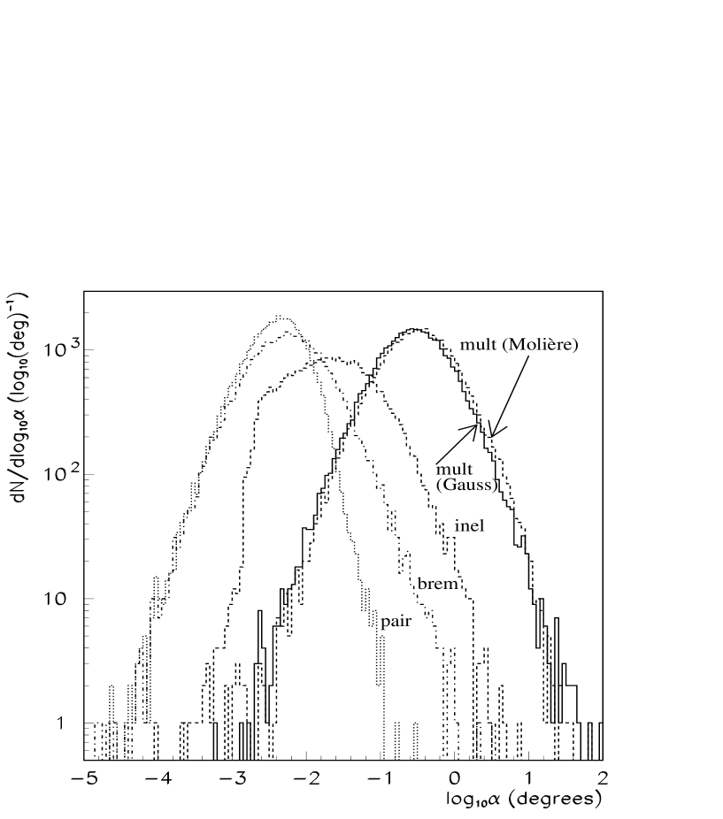
Figure 6: Angular deviations generated by each mechanism of deflection separately at 3 km.w.e. (from a power spectrum with index $\gamma$ = 3.7): multiple scattering (continuous: Gaussian theory, dashed: Molière theory), inelasting scattering (dashed), bremsstrahlung (dot-dashed), pair production (dotted).

In Figure 6 we show the contribution of each process to the angular deviation of muons which pass 3 km.w.e. To do this plot we have repeated five times the same simulation leaving active one mechanism of deflection each time. For multiple scattering we have used either Gaussian treatment described in previous section or Molière theory subroutines provided by GEANT [19]. A more detailed treatment (Molière theory) results in the similar distribution compared with that of Gaussian treatment, with a small increase of mean deflection angle. However, the original Molière theory (see [19] and references therein) does not provide the lateral displacement, more important from the experimental point of view. As can be clearly seen from Figure 6 the multiple scattering dominates over other processes. This result remains true for 10 km.w.e. and for a monochromatic beam of 10 TeV muons.

To calculate survival probabilities, $P(E_{0},h)$, and muon energy distributions underground, $P(E_{0},h,E)$, we have propagated muons with different initial energy (100000 muons for each initial energy) through the standard rock. $P(E_{0},h,E)$ means the probability that muon with initial energy $E_{0}$ will reach the depth $h$ with energy $E$. Figure 7 shows the survival propabilities obtained with MUSIC for $E_{0}$ from 1 to $10^{4}$ TeV. Figure 8 shows $P(E_{0},h)$ for h = 4 km.w.e. and h = 10 km.w.e., calculated with MUSIC and with PROPMU. The curves are very similar also in this case. Our values are on average (1-2)% lower: this difference can be due to the new cross-section for bremsstrahlung used in MUSIC.

We have studied the effects of the cross-section difference and of the stochasticity of different processes on the characteristics of the muon flux underground. Using the sea-level vertical muon energy spectrum, proposed by T.Gaisser [21] with the spectral index of primary spectrum $\gamma=2.70$, and the distributions $P(E_{0},h)$ and $P(E_{0},h,E)$ we have calculated the vertical muon intensities $I(h)$ and mean muon energies $<E(h)>$ at different depths underground:

$$I(h)=\int_{0}^{\infty}P(E_{0},h)\cdot{{dI(E_{0})}\over{dE_{0}}}\cdot dE_{0},$$ (6)

$$<E(h)>={{\int_{0}^{\infty}E\cdot{{dI(E,h)}\over{dE}}\cdot dE}\over{\int_{0}^{\infty}{{dI(E,h)}\over{dE}}\cdot dE}}$$ (7)

where ${{dI(E_{0})}\over{dE_{0}}}$ is the vertical muon energy spectrum at sea level and ${{dI(E,h)}\over{dE}}$ is the vertical muon spectrum at the depth $h$. The latter one is obtained using the formula:

$${{dI(E,h)}\over{dE}}=\int_{0}^{\infty}P(E_{0},h,E)\cdot{{dI(E_{0})}\over{dE_{0}}}\cdot dE_{0},$$ (8)

We have calculated the muon intensities and mean muon energies for two different muon bremsstrahlung cross-sections (from [4] and [9]) and for two values of $v_{cut}$ ($10^{-3}$ and $10^{-2}$). We have carried out additional tests considering the knock-on electron production and pair production as continuous processes. The results of the calculations are presented in Table 1 for $I(h)$ and Table 2 for $<E(h)>$. The first column in both tables shows the depth in km.w.e. of standard rock. Other columns show the intensity in units $cm^{-2}s^{-1}sr^{-1}$ (Table 1) and the mean muon energy in $GeV$ (Table 2). 2nd column present our basic values calculated with the muon bremsstrahlung cross-section from [4] and $v_{cut}=10^{-3}$. The results obtained with bremsstrahlung cross-section from [9] and $v_{cut}=10^{-3}$ are presented in column 3. The values in column 4 were calculated with the cross-section from [4], $v_{cut}=10^{-3}$ and with continuous energy loss due to knock-on electron production. The simulation related to column 5 has been carried out under the same assumptions as that for column 4 but both knock-on electron and pair production have been treated as continuous processes. Finally, column 6 shows the results of the simulation similar to that for column 4, but with $v_{cut}=10^{-2}$. The accuracy of the values presented in Tables 1 and 2 is of the order of $1\%$.

Table 1: Vertical muon intensities, $I(h)$, in units $cm^{-2}s^{-1}sr^{-1}$ for different depths in the standard rock: column 1 – depth in km.w.e.; column 2 – bremsstrahlung cross-section from [4], $v_{cut}=10^{-3}$, all processes are stochastic; column 3 – bremsstrahlung cross-section from [9], $v_{cut}=10^{-3}$, all processes are stochastic; column 4 – bremsstrahlung cross-section from [4], $v_{cut}=10^{-3}$, continuous energy loss due to knock-on electron production ($e$ – cont.); column 5 – bremsstrahlung cross-section from [4], $v_{cut}=10^{-3}$, continuous energy loss due to knock-on electron production and pair production ($e+p$ – cont.); column 6 – bremsstrahlung cross-section from [4], $v_{cut}=10^{-2}$, continuous energy loss due to knock-on electron production.

$h$	[4]	[9]	[4]	[4]	[4]
km.w.e.	$v_{cut}=10^{-3}$	$v_{cut}=10^{-3}$	$v_{cut}=10^{-3}$	$v_{cut}=10^{-3}$	$v_{cut}=10^{-2}$
			$e$–cont.	$e+p$–cont.	$e$–cont.
1	$1.23\cdot 10^{-6}$	$1.28\cdot 10^{-6}$	$1.22\cdot 10^{-6}$	$1.22\cdot 10^{-6}$	$1.22\cdot 10^{-6}$
2	$1.23\cdot 10^{-7}$	$1.30\cdot 10^{-7}$	$1.21\cdot 10^{-7}$	$1.21\cdot 10^{-7}$	$1.21\cdot 10^{-7}$
3	$2.37\cdot 10^{-8}$	$2.53\cdot 10^{-8}$	$2.33\cdot 10^{-8}$	$2.34\cdot 10^{-8}$	$2.33\cdot 10^{-8}$
4	$5.92\cdot 10^{-9}$	$6.33\cdot 10^{-9}$	$5.79\cdot 10^{-9}$	$5.78\cdot 10^{-9}$	$5.78\cdot 10^{-9}$
5	$1.69\cdot 10^{-9}$	$1.81\cdot 10^{-9}$	$1.65\cdot 10^{-9}$	$1.64\cdot 10^{-9}$	$1.64\cdot 10^{-9}$
6	$5.19\cdot 10^{-10}$	$5.57\cdot 10^{-10}$	$5.04\cdot 10^{-10}$	$5.00\cdot 10^{-10}$	$5.02\cdot 10^{-10}$
7	$1.66\cdot 10^{-10}$	$1.80\cdot 10^{-10}$	$1.62\cdot 10^{-10}$	$1.59\cdot 10^{-10}$	$1.62\cdot 10^{-10}$
8	$5.53\cdot 10^{-11}$	$5.94\cdot 10^{-11}$	$5.36\cdot 10^{-11}$	$5.23\cdot 10^{-11}$	$5.35\cdot 10^{-11}$
9	$1.87\cdot 10^{-11}$	$2.02\cdot 10^{-11}$	$1.82\cdot 10^{-11}$	$1.75\cdot 10^{-11}$	$1.81\cdot 10^{-11}$
10	$6.35\cdot 10^{-12}$	$6.86\cdot 10^{-12}$	$6.19\cdot 10^{-12}$	$5.91\cdot 10^{-12}$	$6.15\cdot 10^{-12}$
11	$2.19\cdot 10^{-12}$	$2.38\cdot 10^{-12}$	$2.15\cdot 10^{-12}$	$2.01\cdot 10^{-12}$	$2.11\cdot 10^{-12}$
12	$7.58\cdot 10^{-13}$	$8.21\cdot 10^{-13}$	$7.43\cdot 10^{-13}$	$6.86\cdot 10^{-13}$	$7.24\cdot 10^{-13}$

Table 2: Mean muon energies at vertical, $<E(h)>$, in $GeV$ for different depths in the standard rock (see caption of Table 1).

$h$	[4]	[9]	[4]	[4]	[4]
km.w.e.	$v_{cut}=10^{-3}$	$v_{cut}=10^{-3}$	$v_{cut}=10^{-3}$	$v_{cut}=10^{-3}$	$v_{cut}=10^{-2}$
			$e$–cont.	$e+p$–cont.	$e$–cont.
1	125	124	123	121	123
2	205	203	203	202	202
3	259	255	257	253	257
4	296	291	294	290	293
5	321	315	319	313	318
6	337	332	337	329	336
7	349	342	348	341	346
8	356	351	356	347	353
9	360	353	360	351	358
10	364	359	364	353	360
11	364	358	364	354	362
12	364	359	364	354	363

Let us first compare the intensities obtained with different assumptions used in the code. The intensities calculated with the muon bremsstrahlung cross-section from [9] are systematically higher (by (4-8)$\%$) than those with the cross-section from [4]. The relative difference slightly increases with depth. If the depth–intensity relation measured in some experiment is used to obtain the power index of the muon energy spectrum at sea level (or the primary spectrum), then, the use of the cross-section from [9] will result in a higher power index (softer muon spectrum) than that with cross-section [4]. The difference can be of the order of 0.01.

The treatment of the knock-on electron production and pair production as continuous processes results in the decrease of muon intensities (up to $10\%$ at high depths). The relative difference also increases with depth. The power index of the primary spectrum which can be evaluated from the underground measurements will be lower in this case. The difference in the power index is negligible if only knock-on electron production is treated as a continuous process but can be of the order of 0.02 if both knock-on electron and pair production are not treated stochastically.

The increase of $v_{cut}$ from $10^{-3}$ up to $10^{-2}$ results in a small decrease of the muon intensities ($(2-3)\%$). However, the increase of the relative difference with depth is small and may not influence much the power index which can be evaluated from the measured depth – intensity relation. The increase of power index in this case should not exceed 0.01.

All aforementioned treatments lead to the conclusion that the reasonable cross-sections and assumptions used in the code (may be with the exception of the continuity of the pair production process) result in the muon intensities which do not differ much from each other. The difference is comparable with the systematic uncertainty which can be attributed to the existing experimental data. The difference in the power index of primary spectrum which can be evaluated from the experimental data using calculated intensities should be less than the errors (including systematical error) of the existing data. However, the stochasticity of pair production is quite important for this purpose.

We would like to note that these considerations are attributed to the single muons. The situation can change for multiple muons when the small decrease of the muon survival probability can result in the significant decrease of the intensity of muon bundles with large multiplicity. In section 4 we present some investigations of this point.

The mean muon energies calculated with our basic assumptions (2nd column of Table 2) are higher than those obtained with another cross-section and/or other assumptions. The difference is not negligible in the cases of the cross-section from [9] and/or the continuity of the pair production process.

We have carried out also the simulation of muon transport with our basic assumptions and with $v_{cut}=3\cdot 10^{-4}$. We observed no statistically significant difference in the muon intensities and mean muon energies comparing with those obtained with $v_{cut}=10^{-3}$. We can conclude that our basic assumptions are optimal from the point of view of the correctness of the results and CPU time.

We have checked also the influence of the cross-section difference and $v_{cut}$ on the angular and lateral distributions. The initial sea–level muon spectrum in the power-law form with power index 3.7 has been used. With the cross-section from [4] we have obtained the mean angular deviation 0.56^∘ and 0.45^∘ for 3 and 10 km.w.e., respectively, while with the cross-section from [9] the values are 0.56^∘ and 0.46^∘. Statistical uncertainty is of the order of 0.01^∘. The mean lateral displacement is 1.56 m and 1.87 m with the cross-section from [4] for 3 and 10 km.w.e., respectively, and 1.59 m and 1.93 m with the cross-section from [9]. Statistical uncertainty is about 0.01 m. We can conclude that the difference in the cross-sections does not influence much the angular and lateral distributions at any depth. A small but statistically significant difference of the mean lateral displacements at large depth can be attributed to the difference of the mean muon energies at this depth (see Table 2 and Eq. (5)).

We have carried out also the propagation of muons with $v_{cut}=10^{-2}$. Actually, the increase of $v_{cut}$ from $10^{-3}$ to $10^{-2}$ results in an increase of the average step between two consecutive interactions by one order of magnitude. Thus, this procedure allows us to test the dependence of the resulting angular deviation and lateral displacement on the step between two consecutive interactions. We didn’t find any significant difference between the results with $v_{cut}=10^{-3}$ and $v_{cut}=10^{-2}$. This proves the correctness of the three-dimensional simulation procedure.

4 Muon multiplicity

We have roughly investigated also the effect of bremsstrahlung cross-section on muon multiplicity distribution. We have used the code CORSIKA [10] to simulate the development of a shower produced by a primary cosmic-ray nucleus in atmosphere. We have sampled two sets of 10000 showers produced by protons and iron nuclei of 10⁴ TeV to have a good statistics of muons.

To transport shower muon component through 3000 m.w.e. of standard rock with MUSIC, we have used two cross sections for bremsstrahlung from [9] and [4]. For the case of infinite underground detector, we have produced two muon multiplicity distributions obtained with different cross-sections. Figures 9 and 10 show these distributions for showers produced by protons and iron nuclei. In Table 3 the mean values $<N_{\mu}>$ are presented, their percentage difference $\frac{<N_{\mu BB}>-<N_{\mu KKP}>}{<N_{\mu KKP}>}$ is $\sim 4\%$.

Table 3: Mean muon multiplicity at 3 km.w.e. for proton and iron primaries of energy $10^{4}$ TeV obtained using different bremsstrahlung cross-sections.

$Cross-section$	$<N_{\mu}>\ p$	$<N_{\mu}>\ Fe$
[4]	$7.89\pm 0.04$	$20.96\pm 0.07$
[9]	$8.20\pm 0.04$	$21.71\pm 0.07$

In order to evaluate the possibility that the differences between distributions could be caused by statistical fluctuactions, we have done a $\chi^{2}$ test: the probability that muon multiplicity distributions obtained with different cross sections come from a single distribution is $\sim 10\%$.

The effect of different bremsstrahlung cross sections on muon multiplicity can be underlined using a fit with a negative binomial [22]. It is evident, as shown in Fig. 11, that fit to muon multiplicity distribution, obtained with cross-section from [9], is practically a translation of the other fit due to different values of $<N_{\mu}>$.

These simple considerations proves that the muon interaction cross-sections can influence the muon multiplicity distributions underground and, hence, the primary cosmic-ray composition which can be evaluated from the underground measurements.

In real experiments, however, the observed multiplicity distribution is driven by the primary energy spectrum and the assumed primary composition and a such complete simulation to investigate the differences due to the muon cross sections is beyond the aim of this paper. We can state only that the effect is quite small (but not negligible) and dominated by other systematic uncertainties.

5 Conclusions

We have presented the new three-dimensional Monte-Carlo code MUSIC for muon propagation through the rock. The main advantages of this code are: i) the treatment of all main processes of muon interaction with matter (bremsstrahlung, inelastic scattering, pair production and knock-on electron production) with the fractional energy loss $v>10^{-3}$ as stochastic processes; ii) the use of the most accurate cross-sections of muon interactions with matter; iii) the accounting of the angular deviation of muons due to stochastic processes. We can conclude that the angular and lateral distributions of muons at any depth are fully determined by multiple Coulomb scattering, while other processes give a contribution which is 1-2 orders of magnitudes less. However, the very rare processes of muon scattering to large angles (for example, backward scattering) which can be due to inelastic scattering and/or bremsstrahlung need more accurate treatment of these processes at large $Q^{2}$. We have studied the dependence of the characteristics of muon flux underground on the bremsstrahlung cross-section and assumptions used in the code. We can conclude that the treatment of pair production as a stochastic process is quite important for the characteristics of muon flux underground. The separation of stochastic and continuous energy losses at $v_{cut}=10^{-3}$ is optimal from the point of view of CPU time and the accuracy of the results. The accurate knowledge of the cross-sections is needed to calculate the intensity of single muons and muon bundles underground. Even a small (1-2)% increase of the muon bremsstrahlung cross-section [4] comparing with that from [9] results in a significant (6%) decrease of the single muon intensity at 3 km.w.e. and in a shift (however, quite small) of muon multiplicity distributions toward low multiplicities. This could produce some bias in the interpretation of the muon ’depth–intensity relation’ and multiplicity distribution measured in an underground experiment when they are analysed in terms of the primary spectrum and composition.

6 Acknowledgements

We are grateful to Profs. G.Navarra, O.G.Ryazhskaya, and Drs. P.Lipari, R.P.Kokoulin and G.Battistoni for useful discussions. This work is supported by Italian Institute for Nuclear Physics (INFN), Italian Ministry of University and Scientific-Technological Research (MURST), Russian State Committee of Science and Technologies and Russian Fund of Fundamental Researches (grant 96-02-19007).

Appendix A. Simulation of muon angular deviation due to stochastic processes

To sample the deflection angle of muon due to bremsstrahlung or pair production processes we followed the approximations for mean angle $<\theta^{2}>^{1/2}$ between the incident and scattered muon proposed in [12].

Let us consider first the muon bremsstrahlung process. Since for both energy loss and angular deviation the so-called ’coherent nuclear bremsstrahlung’ [17, 12] is the most important, we have used the parametrisation for $<\theta^{2}>^{1/2}$ of [12] for this process:

$$<\theta^{2}>^{1/2} = \left[\left(k_{1}v^{1/2},k_{2}\right)_{min},k_{3}v\right]_{max},v\leq 0.5$$

$$= k_{4}v^{1+n}(1-v)^{-n},<\theta^{2}>^{1/2}<0.2,v>0.5$$

$$= k_{5}(1-v)^{-1/2},<\theta^{2}>^{1/2}\geq 0.2,v>0.5$$

where $k_{1}=0.092E^{-1/3}$, $k_{2}=0.052E^{-1}Z^{-1/4}$, $k_{3}=0.22E^{-0.92}$, $k_{4}=0.26E^{-0.91}$, $n=0.81E^{1/2}/(E^{1/2}+1.8)$, and $k_{5}$ is related to $k_{4}$ by continuity of the function.

The mean angle between incident and scattered muon due to pair production process has been parametrised as [12]:

$$<\theta^{2}>^{1/2} = (2.3+\ln E)E^{-1}(1-v)^{-1}(v-2m_{e}/E)^{2}v^{-2}$$ (10)

$$\times \left[8.9\cdot 10^{-4}v^{1/4}(1+1.5\cdot 10^{-5}E)+0.032v/(v+1),0.1\right]_{min}$$

where $m_{e}$ is the electron mass.

For a given value of $v$ sampled according to the cross-sections from [4, 11] without any additional approximation the mean angle $<\theta^{2}>^{1/2}$ between incident and scattered muon has been calculated using the Eqs. (9,10). The spatial angle $\theta$ has been chosen from an exponential in the variable $\theta^{2}$ with the mean value $<\theta^{2}>$.

We note again that we did not use any additional parametrisation for the muon inelastic scattering cross-section which has been taken from [16]. For a given value of $v$ sampled according to the cross-section integrated over $Q^{2}$, the muon scattering angle $\theta$ has been simulated using the double-differential cross-section.

For all stochastic processes we have sampled randomly the angle $\phi$ in the plane perpendicular to the muon direction.

The code is available upon the request by e-mail to: antonioli@bo.infn.it or kudryavtsev@vaxmw.tower.ras.ru

Figure 1: Energy distributions of muons (from a power spectrum with index $\gamma$ = 3.7) at 3 km.w.e. (solid line) and at 10 km.w.e. (dashed line).

Figure 2: Angular distributions of muons (from a power spectrum with index $\gamma$ = 3.7) at 3 km.w.e. (solid line) and at 10 km.w.e. (dashed line).

Figure 3: Lateral distributions of muons (from a power spectrum with index $\gamma$ = 3.7) at 3 km.w.e. (solid line) and at 10 km.w.e. (dashed line).

Figure 4: Comparison of angular distributions obtained with MUSIC (solid line) and PROPMU (dashed line) at 3 km.w.e.

Figure 5: Comparison of lateral distributions obtained with MUSIC (solid line) and PROPMU (dashed line) at 3 km.w.e.

Figure 7: Survival probabilities obtained with MUSIC for $E_{0}$ from 1 to 10⁴ TeV.

Figure 8: Comparison between survival probabilities obtained with MUSIC (solid line) and PROPMU (dashed line) at 4 km.w.e. and 10 km.w.e.

Figure 9: Comparison of muon multiplicity distributions at 3 km.w.e. obtained using bremsstrahlung cross sections from [9] (open circles) and [4] (triangles). Muons are produced in 10000 proton showers of energy $E_{o}$ $=$ 10⁴ TeV

Figure 10: Comparison of muon multiplicity distributions at 3 km.w.e obtained using bremsstrahlung cross sections from [9] (open circles) and [4] (triangles). Muons are produced in 10000 showers initiated by iron nuclei of energy $E_{o}$ $=$ 10⁴ TeV

Figure 11: Comparison of the fits to the multiplicity distributions with negative binomial functions. Multiplicity distributions have been obtained using muon bremsstrahlung cross sections from [9] (dashed line) and [4] (solid line) for proton and iron primaries.

References

- [1] H.Bilokon et al., Proc. 20th Intern. Cosmic Ray Conf. (Moscow) 9 (1987) 199. H.Bilokon et al., Nucl. Inst. and Meth. A303 (1991) 381.
- [2] P.Lipari and T.Stanev, Phys. Rev. D 44 (1991) 3543.
- [3] H.Bilokon et al., Preprint LNGS 94/92 (1994).
- [4] S.R.Kelner, R.P. Kokoulin and A.A.Petrukhin, to be published in Physics of Atomic Nuclei (1997).
- [5] V.A.Kudryavtsev, Preprint INR, P-0529 (1987) (in Russian), unpublished.
- [6] M.Aglietta et al. (LVD Collaboration), Astropart. Phys. 3 (1995) 311.
- [7] M.Aglietta et al. (LVD Collaboration), Proc. 24th Intern. Cosmic Ray Conf. (Rome) 1 (1995) 557.
- [8] C.Ghetti, Tesi di Laurea, Bologna University (1996) (in Italian), unpublished.
- [9] L.B.Bezrukov and E.V.Bugaev, Proc. 17th Intern. Cosmic Ray Conf. (Paris) 7 (1981) 102.
- [10] J.N. Capdevielle et al., The Karlsruhe Extensive Air Shower Simulation Code CORSIKA, Kernforschungszentrum Karlsruhe, KfK 4998 (1992).
- [11] R.P. Kokoulin and A.A.Petrukhin, Proc. 12th Intern. Cosmic Ray Conf. (Hobart) 6 (1971) 2436.
- [12] A. Van Ginneken, Nucl. Instr. and Meth. A251 (1986) 21.
- [13] GEANT Detector description and manual, CERN, (Geneva) (1994) PHYS451.
- [14] GEANT Detector description and manual, CERN, (Geneva) (1994) PHYS441.
- [15] H.Inazawa and K.Kobayakawa, Proc. 17th Intern. Cosmic Ray Conf. (Paris) 7 (1981) 94.
- [16] L.B.Bezrukov and E.V.Bugaev, Sov. J. Nucl. Phys. 33 (1981) 635. L.B.Bezrukov and E.V.Bugaev, Sov. J. Nucl. Phys. 32 (1980) 847.
- [17] L. W. Mo and Y.S. Tsai, Review of Modern Phys. 41 (1969) 205.
- [18] G. Battistoni et al., private communication.
- [19] GEANT Detector description and manual, CERN, (Geneva) (1994) PHYS325.
- [20] B.Rossi, High energy particles, Prentice Hall, Englewood Cliffs, NJ (1952).
- [21] T.K.Gaisser, Cosmic Rays and Particle Physics, Cambridge University Press, (1990).
- [22] C. Forti et al., Phys. Rev. D 42 (1990) 3668.