hep-ph/9705398

Single-Top-Quark Production via $W$-Gluon Fusion
at Next-to-Leading Order

T. Stelzer, Z. Sullivan and S. Willenbrock

Department of Physics

University of Illinois

1110 West Green Street

Urbana, IL  61801

Single-top-quark production via $W$-gluon fusion at hadron colliders provides an opportunity to directly probe the charged-current interaction of the top quark. We calculate the next-to-leading-order corrections to this process at the Fermilab Tevatron, the CERN Large Hadron Collider, and DESY HERA. Using a $b$-quark distribution function to sum collinear logarithms, we show that there are two independent corrections, of order $1/\ln(m_{t}^{2}/m_{b}^{2})$ and $\alpha_{s}$. This observation is generic to processes involving a perturbatively derived heavy-quark distribution function at an energy scale large compared with the heavy-quark mass.

1 Introduction

Now that the existence of the top quark is firmly established [1], attention turns to testing its properties. A powerful probe of the charged-current weak interaction of the top quark at hadron colliders is single-top-quark production. The two primary processes are quark-antiquark annihilation via a virtual $s$-channel $W$ boson [2, 3] and $W$-gluon fusion, which involves a virtual $t$-channel $W$ boson (Fig. 1) [4, 5, 6]. Within the context of the standard model, these processes provide a direct measurement of the Cabbibo-Kobayashi-Maskawa matrix element $V_{tb}$. Beyond the standard model, they are sensitive to new physics associated with the charged-current weak interaction of the top quark [7, 8, 9, 10, 11, 12, 13, 14].

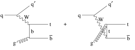
Figure 1: Single-top-quark production via $W$-gluon fusion.

Both the precise measurement of $V_{tb}$ and the indirect detection of new physics require an accurate calculation of the single-top-quark production cross section. The quark-antiquark-annihilation cross section has been calculated at next-to-leading order in QCD, with a theoretical uncertainty of $\pm 6\%$ [15]. The purpose of this article is to calculate the next-to-leading-order correction to the $W$-gluon-fusion cross section.

A complete calculation of the next-to-leading order correction to $W$-gluon fusion has already been presented in the literature [16]. However, we show that this calculation is incorrect, due to the factorization scheme used to subtract collinear divergences. We argue that the CTEQ $b$-quark distribution function used in that calculation [17], although nominally in the deep-inelastic scattering (DIS) scheme, is actually not compatible with that scheme, and yields incorrect results. To avoid this problem, we perform our calculation entirely in the modified minimal subtraction ($\overline{\rm MS}$) scheme [18]. Our numerical results differ significantly from those of Ref. [16].

We make several other contributions to the calculation of the next-to-leading-order correction to the $W$-gluon-fusion process:

1. We show that there are two independent corrections, of order $1/\ln(m_{t}^{2}/m_{b}^{2})$ and $\alpha_{s}$, which are numerically comparable. The leading-order process is $qb\to q^{\prime}t$, as shown in Fig. 2(a). The $1/\ln(m_{t}^{2}/m_{b}^{2})$ correction is associated with the diagrams in Figs. 2(b), 2(c), while the $\alpha_{s}$ correction arises from the diagrams in Figs. 3,4. The existence of a correction of order $1/\ln(\mu^{2}/m_{Q}^{2})$ is a generic feature of calculations involving perturbatively-derived heavy-quark distribution functions at an energy scale $\mu$ large compared with the heavy-quark mass $m_{Q}$.

2. We perform the calculation in a simple and systematic way using a structure-function approach [19, 20]. This allows the calculation to be organized in a straightfoward manner, making use of its similarity with deep-inelastic scattering.

3. We carefully analyze the appropriate scale in the parton distribution functions. We show that the correct scale in the light-quark distribution function is $\mu^{2}=Q^{2}$ ($Q^{2}$ is the virtuality of the $W$ boson), with essentially no scale uncertainty. However, the appropriate scale in the $b$ distribution function is $\mu^{2}\approx Q^{2}+m_{t}^{2}$.

The paper is organized as follows. In Sec. 2 we show that the next-to-leading-order corrections are of two types, $1/\ln(m_{t}^{2}/m_{b}^{2})$ and $\alpha_{s}$. We then argue that these corrections are most reliably calculated in the $\overline{\rm MS}$ factorization scheme. In Sec. 3 we introduce the structure-function approach to calculating these corrections. In Sec. 4 we give our numerical results and draw conclusions. We give results for the Fermilab Tevatron $p\bar{p}$ collider for $\sqrt{S}=$ 1.8 and 2 TeV, the CERN Large Hadron Collider (LHC), a $pp$ collider with $\sqrt{S}=$ 14 TeV, and the DESY $ep$ collider HERA with $\sqrt{S}=314$ GeV. The analytic expressions for the next-to-leading-order structure functions are gathered in the Appendix.

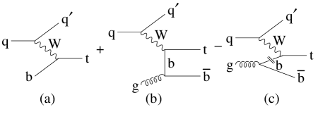
Figure 2: (a) Leading-order process for single-top-quark production, using a $b$ distribution function. (b) Correction to the leading-order process from an initial gluon. (c) Subtracting the collinear region from (b), corresponding to a gluon splitting into a $b\bar{b}$ pair. (b) and (c) taken together constitute a correction of order $1/\ln(m_{t}^{2}/m_{b}^{2})$ to the leading-order process in (a).

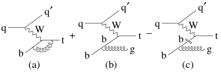
Figure 3: Order $\alpha_{s}$ correction to the heavy-quark vertex in the leading-order process $qb\to q^{\prime}t$. (c) represents the subtraction of the collinear region from (b).

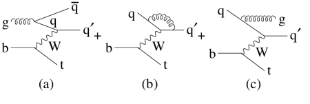
Figure 4: Order $\alpha_{s}$ correction to the light-quark vertex in the leading-order process $qb\to q^{\prime}t$.

2 Next-to-leading-order corrections

2.1 $1/\ln(m_{t}^{2}/m_{b}^{2})$ correction

The tree-level diagrams for $W$-gluon fusion are shown in Fig. 1. Since the $b$-quark mass is small compared with $m_{t}$, let us neglect it for the moment. If the $b$ quark is massless, the first of these diagrams is singular when the final $\bar{b}$ quark is collinear with the incoming gluon. This kinematic configuration corresponds to the incoming gluon splitting into a real $b\bar{b}$ pair. The propagator of the internal $b$ quark in the diagram is therefore on-shell, and is infinite.

In reality the $b$ quark is not massless, and its mass regulates the collinear singularity which exists in the massless case. The collinear singularity manifests itself in the total cross section as terms proportional to $\ln[(Q^{2}+m_{t}^{2})/m_{b}^{2}]$, where $Q^{2}\equiv-q^{2}$ is the virtuality of the $W$ boson of four-momentum $q$. Since the virtuality of the $W$ boson is controlled by the $W$ propagator, $Q^{2}$ is typically less than or of order $M_{W}^{2}$. For readability, we write the logarithm as $\ln(m_{t}^{2}/m_{b}^{2})$ in the following discussion (since $m_{t}^{2}\gg M_{W}^{2}$), although we use the exact expression in all calculations.

The total cross section for $W$-gluon fusion contains these logarithmically enhanced terms, of order $\alpha_{s}\ln(m_{t}^{2}/m_{b}^{2})$, as well as terms of order $\alpha_{s}$ (both terms also carry a factor of $\alpha_{W}^{2}$, which we suppress in the following discussion). Furthermore, logarithmically enhanced terms, of order $\alpha_{s}^{n}\ln^{n}(m_{t}^{2}/m_{b}^{2})/n!$, appear at every order in the perturbative expansion in the strong coupling, due to collinear emission of gluons from the internal $b$-quark propagator. Since the logarithm is large, the perturbation series does not converge quickly, and it appears difficult to obtain a precise prediction for the total cross section.

Fortunately, this difficulty can be obviated. A formalism exists to sum the collinear logarithms to all orders in perturbation theory [21, 22, 23]. The coefficient of the logarithmically-enhanced term is the Dokshitzer-Gribov-Lipatov-Altarelli-Parisi (DGLAP) splitting function $P_{qg}$, which describes the splitting of a gluon into a $b\bar{b}$ pair. One can sum the logarithms by introducing a $b$ distribution function $b(x,\mu^{2})$ and calculating its evolution with $\mu$ (from some initial condition) via the DGLAP equations. Thus the $b$ distribution function can be regarded as a device to sum the collinear logarithms. Since it is calculated from the splitting of a gluon into a collinear $b\bar{b}$ pair, it is intrinsically of order $\alpha_{s}\ln(\mu^{2}/m_{b}^{2})$. We elaborate on this point at the end of this section.

Once a $b$ distribution function is introduced, it changes the way one orders perturbation theory. The leading-order process is now $qb\to q^{\prime}t$, shown in Fig. 2(a). This cross section is of order $\alpha_{s}\ln(m_{t}^{2}/m_{b}^{2})$, due to the $b$ distribution function ($\mu\approx m_{t}$). The $W$-gluon-fusion process, shown in Fig. 2(b), contains terms of both order $\alpha_{s}\ln(m_{t}^{2}/m_{b}^{2})$ and $\alpha_{s}$, as discussed above. However, the logarithmically enhanced terms have been summed into the $b$ distribution function and thus are already present in Fig. 2(a). It is therefore necessary to remove these terms from the $W$-gluon fusion process to avoid double counting. This is indicated schematically in Fig. 2(c); the double lines crossing the internal $b$-quark propagator indicate that it is on-shell, which corresponds to the kinematic region responsible for the large collinear logarithm [21, 22, 23].

After the subtraction of the terms of order $\alpha_{s}\ln(m_{t}^{2}/m_{b}^{2})$ in Fig. 2(b) by the terms in Fig. 2(c), the remaining terms are of order $\alpha_{s}$. Compared with the leading-order process in Fig. 2(a), this is suppressed by a factor $1/\ln(m_{t}^{2}/m_{b}^{2})$. Thus the diagrams of Figs. 2(b), 2(c), taken together, correspond to a correction to the leading-order cross section [Fig. 2(a)] of $1/\ln(m_{t}^{2}/m_{b}^{2})$, not of order $\alpha_{s}$. This is an essential point which has been previously overlooked.

This observation is generic to any process involving a perturbatively derived heavy-quark distribution function in the region $\mu^{2}\gg m_{Q}^{2}$. For example, the calculation analogous to the diagrams in Figs. 2(b), 2(c) for charm production in neutral-current deep inelastic scattering [23] corresponds to a correction of order $1/\ln(Q^{2}/m_{c}^{2})$ for $Q^{2}\gg m_{c}^{2}$.

Let us elaborate on our contention that the $b$ distribution function is intrinsically of order $\alpha_{s}\ln(\mu^{2}/m_{b}^{2})$, rather than merely of order $\alpha_{s}$. If one neglects gluon bremsstrahlung and the scale dependence of the gluon distribution function and the strong coupling, one can solve the DGLAP equation for the $b$ distribution function analytically [with the initial condition $b(x,\mu^{2})=0$ at $\mu=m_{b}$] [21, 22, 23]:

$$b(x,\mu^{2})=\frac{\alpha_{s}(\mu^{2})}{2\pi}\ln\left(\frac{\mu^{2}}{m_{b}^{2}}\right)\int_{x}^{1}\frac{dz}{z}P_{qg}(z)g\left(\frac{x}{z},\mu^{2}\right)\;,$$ (1)

where the DGLAP splitting function is given by

$$P_{qg}(z)=\frac{1}{2}[z^{2}+(1-z)^{2}]\;.$$ (2)

Equation (1) shows that $b(x,\mu^{2})$ is of order $\alpha_{s}\ln(\mu^{2}/m_{b}^{2})$ compared with the gluon distribution function. To support this, we show in Fig. 5 the ratio $b(x,\mu^{2})/g(x,\mu^{2})\times 2\pi/\alpha_{s}(\mu^{2})$ as a function of $\mu$ for various fixed values of $x$, using the CTEQ4M parton distribution functions [24]. The curves are approximately linear when $\mu$ is plotted on a logarithmic scale, indicating that $b(x,\mu^{2})\propto[\alpha_{s}(\mu^{2})/2\pi]\ln(\mu^{2}/m_{b}^{2})g(x,\mu^{2})$.

Figure 5: The ratio of the $b$ distribution function to the gluon distribution function, times $2\pi/\alpha_{s}(\mu^{2})$, versus the factorization scale $\mu$, for various fixed values of $x$. The curves are approximately linear when $\mu$ is plotted on a logarithmic scale, indicating that $b(x,\mu^{2})\propto[\alpha_{s}(\mu^{2})/2\pi]\ln(\mu^{2}/m_{b}^{2})g(x,\mu^{2})$, as suggested by the approximation of Eq. (1).

The $b$ distribution function is on a different footing from the light-quark distribution functions. The light-quark distribution functions involve nonperturbative QCD, and must be measured (or calculated nonperturbatively). The $b$ distribution function involves energies of order $m_{b}$ and larger, so it can be calculated perturbatively; no measurement is necessary. Given the gluon and light-quark distributions functions, perturbative QCD makes a definite prediction for the $b$ distribution function.

2.2 $\alpha_{s}$ correction

There are also bona fide $\alpha_{s}$ corrections to the leading-order process $qb\to q^{\prime}t$. The diagram in Fig. 3(a) is such a correction; it is of order $\alpha_{s}^{2}\ln(m_{t}^{2}/m_{b}^{2})$ [including the factor $\alpha_{s}\ln(m_{t}^{2}/m_{b}^{2})$ from the $b$ distribution function], so it is suppressed by a factor of $\alpha_{s}$ with respect to the leading-order process.

The diagram of Fig. 3(b) contains terms of both order $\alpha_{s}^{2}\ln^{2}(m_{t}^{2}/m_{b}^{2})$ and $\alpha_{s}^{2}\ln(m_{t}^{2}/m_{b}^{2})$. The former terms arise from the collinear emission of the gluon, which gives rise to another factor of $\ln(m_{t}^{2}/m_{b}^{2})$ (on top of the factor from the $b$ distribution function). Similar to the discussion above, another power of this logarithm appears at every order in the strong coupling, and summation is required to improve the convergence of perturbation theory. The coefficient of this logarithmically enhanced term is the DGLAP splitting function $P_{qq}$, which describes the splitting of a quark into a quark and a gluon. The collinear logarithms are summed by adding another term, corresponding to gluon emission, to the DGLAP evolution equation for the $b$ distribution function. Once this is done, the collinear region must be subtracted from Fig. 3(b); this is shown schematically in Fig. 3(c). The remaining terms are of order $\alpha_{s}^{2}\ln(m_{t}^{2}/m_{b}^{2})$, so they are bona fide $\alpha_{s}$ corrections to the leading-order process.

Finally, there are the corrections to the light-quark vertex in the leading-order process, as shown in Fig. 4. These are also bona fide $\alpha_{s}$ corrections. Figs. 4(a), 4(b) contain collinear logarithms $\ln(Q^{2}/m_{q}^{2})$ (where $m_{q}$ is a light-quark mass) which are absorbed by the light-quark distribution functions in the usual way. Since the light-quark distribution functions are intrinsically of zeroth order in $\alpha_{s}$, the remaining corrections are of order $\alpha_{s}$.

2.3 Higher orders

Consider the next-to-next-to-leading order diagram in Fig. 6. This diagram generates terms of order $\alpha_{s}^{2}\ln^{2}(m_{t}^{2}/m_{b}^{2})$, $\alpha_{s}^{2}\ln(m_{t}^{2}/m_{b}^{2})$, and $\alpha_{s}^{2}$. The term of order $\alpha_{s}^{2}\ln^{2}(m_{t}^{2}/m_{b}^{2})$ comes from the region in which the initial gluon splits into a collinear $b\bar{b}$ pair, and the $b$ quark subsequently radiates a collinear gluon. This term is summed by the leading-order DGLAP equation, which sums leading logarithms $\alpha_{s}^{n}\ln^{n}(m_{t}^{2}/m_{b}^{2})/n!$, as discussed in Sec. 2.1. Thus this term is already present in the leading-order diagram, Fig. 2(a).

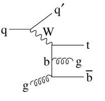
Figure 6: Next-to-next-to-leading-order contribution to single-top-quark production via $W$-gluon fusion.

The terms of order $\alpha_{s}^{2}\ln(m_{t}^{2}/m_{b}^{2})$ come from two sources. The first is when the initial gluon splits into a collinear $b\bar{b}$ pair, and the $b$ quark subsequently radiates a noncollinear gluon. This is associated with the diagrams in Figs. 3(b) and 3(c), taken together, which correspond to noncollinear gluon radiation. The logarithm is summed via the leading-order DGLAP equation into the $b$ distribution function in Figs. 3(b), 3(c), so this term is already accounted for.

The other term of order $\alpha_{s}^{2}\ln(m_{t}^{2}/m_{b}^{2})$ is summed by extending the DGLAP splitting function $P_{qg}$ to next-to-leading order. This sums the first subleading logarithms, of order $\alpha_{s}^{n}\ln^{n-1}(m_{t}^{2}/m_{b}^{2})$ ($n\geq 2$) into the $b$ distribution function of the leading-order process, Fig. 2(a). The remaining term, of order $\alpha_{s}^{2}$, is a correction of order $\alpha_{s}\times 1/\ln(m_{t}^{2}/m_{b}^{2})$ compared with the leading order process of Fig. 2(a).

This analysis demonstrates that all collinear logarithms are ultimately summed into the $b$ distribution function; no explicit collinear logarithms remain. The remaining terms are all of order $\alpha_{s}^{n}$ or, if the diagram has a $b$ quark in the initial state, of order $\alpha_{s}^{n}\ln(m_{t}^{2}/m_{b}^{2})$. These correspond to corrections of order $\alpha_{s}^{n-1}\times 1/\ln(m_{t}^{2}/m_{b}^{2})$ or $\alpha_{s}^{n-1}$, respectively, compared with the leading-order process. For a more detailed discussion of higher orders, see Ref. [25].

2.4 Factorization scheme for heavy quarks

The factorization scheme used to eliminate the collinear divergences from the parton cross section must be the same as the scheme used to define the parton distribution functions in order to yield a correct (and scheme-independent) result. In the $\overline{\rm MS}$ scheme, the $b$ distribution function $b(x,\mu^{2})$ is defined to be zero at $\mu=m_{b}$, and is then evolved to higher values of $\mu$ via the DGLAP equations [18]. This is the definition of the $b$ distribution function employed in the CTEQ $\overline{\rm MS}$ parton distribution functions [17, 24].

Another popular factorization scheme is the DIS scheme. In this scheme, the neutral-current structure function $F_{2}(x,Q^{2})$ is defined to have no radiative correction for light quarks. For $\mu\gg m_{b}$, the $b$ quark is essentially a light quark, so a natural interpretation of the DIS scheme for the $b$ quark is that its contribution to $F_{2}(x,Q^{2})$ has no radiative correction. This is the interpretation that was made in Ref. [16], which adopted the DIS scheme for the parton cross section and used the CTEQ DIS distribution functions [17]. However, the CTEQ DIS $b$ distribution function is actually not in the DIS scheme as interpreted in Ref. [16]. Rather, the $b$ distribution function is again defined by the initial condition $b(x,\mu^{2})=0$ at $\mu=m_{b}$, and evolved to higher values of $\mu$ via the DGLAP equations. There is no sense in which this yields a $b$ distribution function which is formally equivalent to the usual DIS scheme. As a consequence, it is not correct to calculate the parton cross section in the usual DIS scheme when using the CTEQ DIS $b$ distribution function. The same is true of the CTEQ DIS charm distribution function.

To avoid this problem, we calculate entirely in the $\overline{\rm MS}$ scheme. This yields very different numerical results from the calculation of Ref. [16] in the DIS scheme.

3 Structure-function approach

Inspecting the leading-order process in Fig. 2(a), $qb\to q^{\prime}t$, one observes that it is analogous to charged-current deep-inelastic scattering. In fact, it is double deep-inelastic scattering; the virtual $W$ boson is probing both the hadron containing the $b$ quark, and the hadron containing the light quark, $q$. This is shown schematically in Fig. 7. We can exploit this analogy to calculate the corrections to this process in a compact way, in terms of next-to-leading-order hadronic structure functions [19, 20]. This factorization of the process is exact at next-to-leading order, because diagrams involving gluon exchange between the light-quark and heavy-quark lines do not interfere with the tree diagram, due to color conservation.

Figure 7: Single-top-quark production via $W$-gluon fusion from a structure-function point of view. The $W$ boson initiates deep inelastic scattering on both hadrons.

The hadronic tensor describing a $W$ boson of four-momentum $q$ striking a hadron of four-momentum $P$ can be written in terms of five structure functions:

$$MW_{\mu\nu}(x,Q^{2}) = F_{1}(x,Q^{2})\left(-g_{\mu\nu}+\frac{q_{\mu}q_{\nu}}{q^{2}}\right)+\frac{F_{2}(x,Q^{2})}{P\cdot q}\left(P_{\mu}-\frac{P\cdot q}{q^{2}}q_{\mu}\right)\left(P_{\nu}-\frac{P\cdot q}{q^{2}}q_{\nu}\right)$$ (3)

$$\mbox{}-i\frac{F_{3}(x,Q^{2})}{2P\cdot q}\epsilon_{\mu\nu\rho\sigma}P^{\rho}q^{\sigma}+F_{4}(x,Q^{2})q_{\mu}q_{\nu}+F_{5}(x,Q^{2})(P_{\mu}q_{\nu}+P_{\nu}q_{\mu})\;,$$

where $Q^{2}=-q^{2}$. If the struck quark, and the quark into which it is converted, are both massless, then the current with which the $W$ interacts is conserved, and one has $q^{\mu}W_{\mu\nu}=q^{\nu}W_{\mu\nu}=0$. This implies that the structure functions $F_{4},F_{5}$ vanish. The scaling variable $x$ is given by $x=Q^{2}/2P\cdot q$, as usual.

If the quark into which the struck quark is converted is massive, such as the top quark, then the current is no longer conserved, and $F_{4},F_{5}$ are nonvanishing (although we will find that they do not enter our calculation). Furthermore, the scaling variable is now given by $x=(Q^{2}+m_{t}^{2})/2P\cdot q$.

The hadronic cross section in Fig. 7 is obtained by contracting the hadronic tensors at each vertex with the square of the $W$ propagator connecting them. Due to current conservation of the light-quark tensor, the $q^{\mu}q^{\nu}/M_{W}^{2}$ term in the numerator of the $W$ propagator does not contribute, so one simply contracts the two tensors together. One finds

$$MW_{\mu\nu}(x_{1},Q^{2})MW^{\mu\nu}(x_{2},Q^{2})=$$ (4)

$$3F_{1}(x_{1},Q^{2})F_{1}(x_{2},Q^{2})$$

$$\mbox{}+F_{1}(x_{1},Q^{2})F_{2}(x_{2},Q^{2})\frac{P_{2}\cdot(-q)}{q^{2}}+F_{2}(x_{1},Q^{2})F_{1}(x_{2},Q^{2})\frac{P_{1}\cdot q}{q^{2}}$$

$$\mbox{}+F_{2}(x_{1},Q^{2})F_{2}(x_{2},Q^{2})\frac{1}{P_{1}\cdot qP_{2}\cdot(-q)}\left(P_{1}\cdot P_{2}-\frac{P_{1}\cdot qP_{2}\cdot q}{q^{2}}\right)^{2}$$

$$\mbox{}+\frac{1}{2}F_{3}(x_{1},Q^{2})F_{3}(x_{2},Q^{2})\left(\frac{P_{1}\cdot P_{2}q^{2}}{P_{1}\cdot qP_{2}\cdot q}-1\right)\;,$$

where

$$Q^{2} = -q^{2}\;,$$ (5)

$$x_{1} = \frac{Q^{2}}{2P_{1}\cdot q}\;,$$ (6)

$$x_{2} = \frac{Q^{2}+m_{t}^{2}}{2P_{2}\cdot(-q)}\;.$$ (7)

The heavy-quark structure functions $F_{4},F_{5}$ do not contribute to this expression because they are the coefficients of tensors which contain $q^{\mu}$, $q^{\nu}$, or both. These tensors give vanishing contribution when contracted with the light-quark tensor, due to current conservation. The $W$ boson interacts with massless quarks in the hadron of four-momentum $P_{1}$, and interacts with a $b$ quark in the hadron of four-momentum $P_{2}$, as indicated in Fig. 7. Note that the latter hadron is probed by a $W$ boson of four-momentum $-q$, which results in $P_{2}\cdot(-q)$ appearing in several places in Eq. (4). One must also add the contribution where the $W$ boson interacts with massless quarks in the hadron of four-momentum $P_{2}$ and with the $b$ quark in the hadron of four-momentum $P_{1}$.

The differential hadronic cross section is given by [20]

$$d\sigma=\frac{1}{2S}4\left(\frac{g^{2}}{8}\right)^{2}\frac{1}{(Q^{2}+M_{W}^{2})^{2}}MW_{\mu\nu}(x_{1},Q^{2})MW^{\mu\nu}(x_{2},Q^{2})(2\pi)^{2}\frac{1}{4S}dQ^{2}dW_{1}^{2}dW_{2}^{2}\;,$$ (8)

where $W_{1}^{2}=(P_{1}+q)^{2}$ and $W_{2}^{2}=(P_{2}-q)^{2}$ are the squared invariant masses of the hadron remnants (including the top quark), and $S=2P_{1}\cdot P_{2}$ is the square of the hadronic center-of-momentum energy. Using

$$2P_{1}\cdot q = W_{1}^{2}+Q^{2}\;,$$ (9)

$$2P_{2}\cdot(-q) = W_{2}^{2}+Q^{2}\;,$$ (10)

we can write Eq. (4) in terms of the integration variables $Q^{2},W_{1}^{2},W_{2}^{2}$:

$$MW_{\mu\nu}(x_{1},Q^{2})MW^{\mu\nu}(x_{2},Q^{2})=$$ (11)

$$3F_{1}(x_{1},Q^{2})F_{1}(x_{2},Q^{2})$$

$$\mbox{}-\frac{1}{2}F_{1}(x_{1},Q^{2})F_{2}(x_{2},Q^{2})\frac{W_{2}^{2}+Q^{2}}{Q^{2}}-\frac{1}{2}F_{2}(x_{1},Q^{2})F_{1}(x_{2},Q^{2})\frac{W_{1}^{2}+Q^{2}}{Q^{2}}$$

$$\mbox{}+F_{2}(x_{1},Q^{2})F_{2}(x_{2},Q^{2})\frac{1}{(W_{1}^{2}+Q^{2})(W_{2}^{2}+Q^{2})}\left(S-\frac{(W_{1}^{2}+Q^{2})(W_{2}^{2}+Q^{2})}{2Q^{2}}\right)^{2}$$

$$\mbox{}+F_{3}(x_{1},Q^{2})F_{3}(x_{2},Q^{2})\left(\frac{SQ^{2}}{(W_{1}^{2}+Q^{2})(W_{2}^{2}+Q^{2})}-\frac{1}{2}\right)\;,$$

where

$$x_{1} = \frac{Q^{2}}{W_{1}^{2}+Q^{2}}\;,$$ (12)

$$x_{2} = \frac{Q^{2}+m_{t}^{2}}{W_{2}^{2}+Q^{2}}\;.$$ (13)

The physical region is given by

$$W_{1} \geq 0\;,$$ (14)

$$W_{2} \geq m_{t}\;,$$ (15)

$$W_{1}+W_{2} \leq \sqrt{S}\;,$$ (16)

$$Q^{2}_{max\atop min} = \frac{1}{2}[S-W_{1}^{2}-W_{2}^{2}\pm\lambda^{1/2}(S,W_{1}^{2},W_{2}^{2})]\;,$$ (17)

$$\lambda(a,b,c) = a^{2}+b^{2}+c^{2}-2ab-2ac-2bc\;.$$ (18)

The next-to-leading-order expressions for the structure functions are given in the Appendix. We use the $\overline{\rm MS}$ scheme, for the reasons discussed in the previous section. After the subtraction of the collinear logarithms $\ln[(Q^{2}+m_{t}^{2})/m_{b}^{2}]$, we set the $b$ mass to zero, since it is small compared with the top-quark mass. When evaluating the next-to-leading-order contribution to the cross section, we use the next-to-leading-order expression for the structure function corresponding to the light quark or the heavy quark, but not both at the same time, as this would yield a contribution of next-to-next-to-leading order.

Factorization scale

The similarity of the leading-order process $qb\to q^{\prime}t$ with deep inelastic scattering suggests that the relevant scale in the light-quark distribution function is $\mu^{2}=Q^{2}$. If the parton distribution functions were extracted solely from deep-inelastic-scattering data at the same values of $x$ and $Q^{2}$ relevant to this process, this statement would be exactly correct, because the radiative corrections to deep-inelastic scattering are precisely the same as those to the light-quark vertex in $qb\to q^{\prime}t$. The latter process has additional radiative corrections, both to the heavy-quark vertex and between the two quark lines, but these are unrelated to the scale in the light-quark distribution function.

The actual situation is not far from the situation described above. Most of the information on the light-quark distribution functions does come from deep inelastic scattering, and the relevant values of $x$ and $Q^{2}$ are within the range of the HERA $ep$ collider: $x\sim m_{t}/\sqrt{S}\sim 0.1$ at the Tevatron and $x\sim 0.01$ at the LHC, with $Q^{2}{\raise 1.29167pt\hbox{$<$\kern-7.5pt\lower 4.30554pt\hbox{$\sim$}}}M_{W}^{2}$. We therefore set $\mu^{2}=Q^{2}$ in the light-quark distribution function and refrain from varying the scale, as is usually done to estimate the theoretical uncertainty from uncalculated higher-order corrections.

The situation is entirely different for the scale in the $b$ distribution function. The collinear logarithm that results from the diagrams in Figs. 2(b) and 3(b) is $\ln[(Q^{2}+m_{t}^{2})/m_{b}^{2}]$. Upon subtraction of the collinear region via the diagrams in Figs. 2(c) and 3(c), the remaining logarithm is $\ln[(Q^{2}+m_{t}^{2})/\mu^{2}]$ (see the Appendix). The appropriate scale in the $b$ distribution function is therefore $\mu^{2}\approx Q^{2}+m_{t}^{2}$. Since the $b$ distribution is obtained from an entirely theoretical calculation, we vary this scale in order to estimate the uncertainty from uncalculated higher-order corrections.

The argument above shows that the appropriate scales in the light-quark and $b$-quark distribution functions are different. Although it may seem unfamiliar to have different scales in the parton distribution functions of a given hadronic process, we have shown that it is appropriate in this case. The appropriate scale for the production of a quark of mass $m_{Q}$ via charged-current deep inelastic scattering is $\mu^{2}=Q^{2}+m_{Q}^{2}$, which yields $\mu^{2}=Q^{2}$ for the light-quark structure function and $\mu^{2}=Q^{2}+m_{t}^{2}$ for the top-quark charged-current structure function.

4 Results and Conclusions

We evaluate the next-to-leading-order cross section for single-top-quark production via $W$-gluon fusion using the latest CTEQ $\overline{\rm MS}$ distribution functions, CTEQ4M [24]. The cross sections at the Tevatron (1.8 and 2 TeV) and the LHC for the sum of $t$ and $\bar{t}$ production for $m_{t}=$ 175 GeV are given in Table 1, assuming $V_{tb}=1$. The leading-order cross sections are also evaluated with the CTEQ4M distribution functions. (When evaluated with the CTEQ4L leading-order distribution functions, the leading-order cross sections are 1.61, 2.31, and 237 pb at the three machines.) The $1/\ln(m_{t}^{2}/m_{b}^{2})$ and $\alpha_{s}$ corrections are listed separately. The $1/\ln(m_{t}^{2}/m_{b}^{2})$ correction is $-20\%$ at the Tevatron, and $-11\%$ at the LHC. This confirms previous calculations of this correction in the $\overline{\rm MS}$ scheme [7, 30, 31]. The $\alpha_{s}$ correction is $+12\%$ at the Tevatron, and $+2\%$ at the LHC. The next-to-leading-order cross section is the sum of the leading-order cross section and these two corrections. The fact that the $\alpha_{s}$ correction partially compensates the $1/\ln(m_{t}^{2}/m_{b}^{2})$ correction is a numerical accident, as these are two truly independent parameters.

Also given in Table 1 is the cross section for $e^{-}p\to\nu_{e}\bar{t}b$ or $e^{+}p\to\bar{\nu}_{e}t\bar{b}$ at HERA [26, 27, 28]. (The leading-order cross section is $1.21\times 10^{-4}$ pb when evaluated with the CTEQ4L leading-order distribution functions.) The $1/\ln(m_{t}^{2}/m_{b}^{2})$ correction is $-33\%$, and the $\alpha_{s}$ correction is $+36\%$. An integrated luminosity of about 10 fb^-1 would be needed to produce a single event. This is unattainable given the design luminosity of the machine (${\cal L}=1.6\times 10^{31}/cm^{2}/s$).

$\sqrt{S}$		LO (pb)	$1/\ln(m_{t}^{2}/m_{b}^{2})$ (pb)	$\alpha_{s}$ (pb)	NLO (pb)
1.8	TeV $p\bar{p}$	1.84	-0.39	0.25	1.70
2	TeV $p\bar{p}$	2.67	-0.55	0.32	2.44
14	TeV $pp$	270	-31	6	245
314	GeV $ep$	1.02$\times 10^{-4}$	-0.34$\times 10^{-4}$	0.36$\times 10^{-4}$	1.04$\times 10^{-4}$

Table 1: Cross sections for single-top-quark production via $W$-gluon fusion at the Tevatron, LHC, and HERA for $m_{t}=175$ GeV. The cross sections are the sum of $t$ and $\bar{t}$ production at the Tevatron and the LHC, and either $t$ (positron beam) or $\bar{t}$ (electron beam) at HERA. The first column gives the leading-order cross section [Fig. 2(a)]; the second column the correction of order $1/\ln(m_{t}^{2}/m_{b}^{2})$ [Figs. 2(b), 2(c)]; the third column the correction of order $\alpha_{s}$ (Figs. 3,4); and the last column the next-to-leading-order cross section (the sum of the first three columns). All calculations are performed in the ${\overline{\rm MS}}$ scheme using CTEQ4M parton distributions functions with $\mu^{2}=Q^{2}$ for the light-quark vertex and $\mu^{2}=Q^{2}+m_{t}^{2}$ for the heavy-quark vertex.

We argued in Sec. 2.3 that the CTEQ DIS $b$ distribution function is incompatible with the usual DIS scheme, and yields incorrect results. To demonstrate this, we also perform the calculation in the DIS scheme using CTEQ4D distribution functions. The next-to-leading-order cross sections at the Tevatron (1.8 and 2 TeV) and the LHC are found to be 2.24, 3.20, 290 pb. These differ from the results in the $\overline{\rm MS}$ scheme by much more than the theoretical uncertainty in that calculation, which we now estimate.

To estimate the uncertainty from uncalculated higher-order corrections, we vary the scale in the $b$ distribution function about the central value $\mu^{2}=Q^{2}+m_{t}^{2}$. The results are shown in Fig. 8 at the Tevatron (2 TeV) and the LHC, for both the leading-order and next-to-leading-order cross sections, using the CTEQ4M parton distribution functions. The next-to-leading-order cross section is considerably less sensitive to $\mu$, as expected. Varying $\mu$ between one-half and twice its central value yields an uncertainty in the next-to-leading-order cross section of $\pm 5\%$ at the Tevatron and $\pm 4\%$ at the LHC. As discussed in Sec. 3, we do not vary the scale in the light-quark distribution function, where $\mu^{2}=Q^{2}$. Although our estimate of the theoretical uncertainty in the cross section from uncalculated higher orders is rather small, it would be worthwhile to pursue the calculation to the next order in $\alpha_{s}$.

Figure 8: Cross section for single-top-quark production via $W$-gluon fusion at the Tevatron and the LHC for $m_{t}=175$ GeV, versus the ratio of the factorization scale $\mu$ to its natural value, $\mu=\sqrt{Q^{2}+m_{t}^{2}}$. Both the leading-order and next-to-leading-order cross sections are shown.

Another source of uncertainty stems from the uncertainty in the top-quark mass. The cross section as a function of the top-quark mass is shown in Fig. 9 at the Tevatron (2 TeV) and the LHC. The cross section is relatively insensitive to the top-quark mass because the decrease in the parton distribution functions with increasing $m_{t}$ is not augmented by a decrease in the partonic cross section, which scales like $1/M_{W}^{2}$ instead of $1/\hat{s}$. The present uncertainty of $\pm 5.5$ GeV in the top-quark mass [29] corresponds to an uncertainty of $\pm 9\%$ in the cross section at the Tevatron and $\pm 5\%$ at the LHC. Anticipating an uncertainty of $\pm 2$ GeV in the top-quark mass from Run II at the Tevatron and/or from the LHC reduces the uncertainty in the cross section from the top-quark mass to $\pm 3\%$ at the Tevatron and $\pm 2\%$ at the LHC.

Figure 9: Next-to-leading-order cross section for single-top-quark production via $W$-gluon fusion at the Tevatron and the LHC as a function of the top-quark mass.

Another source of uncertainty is the gluon distribution function, which reflects itself in an uncertainty in the $b$ distribution function. It is impossible to estimate this uncertainty with any confidence at this time; what is needed is a parton distribution set with an associated error-correlation matrix.

In this paper we present the first complete and correct calculation of the next-to-leading-order corrections to single-top-quark production via $W$-gluon fusion. We show that there are two independent corrections, of order $1/\ln(m_{t}^{2}/m_{b}^{2})$ and $\alpha_{s}$, which are numerically comparable. We estimate the uncertainty due to uncalculated higher-order corrections to be about $\pm 5\%$ at the Tevatron and the LHC. Assuming the uncertainty in the gluon distribution function can be quantified and reduced to a sufficiently-small level, single-top-quark production via $W$-gluon fusion will be an accurate probe of the charged-current interaction of the top quark at the Tevatron and the LHC. In conjunction with $q\bar{q}\to t\bar{b}$, it will yield an accurate measurement of $V_{tb}$ and possibly indicate the presence of new physics.

Note: The numerical results contained in this paper were obtained by evaluating the weak coupling constant $g$ in terms of the Fermi coupling $G_{F}$ and the $W$-boson mass $M_{W}$, via $g^{2}=8G_{F}M_{W}^{2}/\sqrt{2}$, where $G_{F}=1.16639\times 10^{-5}$ GeV^-2 and $M_{W}=80.4$ GeV. These numerical results are approximately $2\%$ less than the values which appear in the published version of this paper [Phys. Rev. D 56, 5919 (1997)].

Appendix

The structure functions for the charged-current production of a heavy quark were calculated at next-to-leading order many years ago in Ref. [32]. This calculation was recently repeated in Ref. [33], which discovered a misprint in the previous result, and also adopted the modern convention of treating the gluon as having $N-2$ helicity states in $N$ dimensions. We present the structure functions below, for completeness.

Our calculation utilizes the charged-current structure functions for top-quark production, $F_{i}(x,Q^{2})$ ($i=1,2,3$), calculated in the $\overline{\rm MS}$ scheme. The bottom-quark mass is neglected throughout. To make contact with Refs. [32, 33] we define a related set of structure functions, ${\cal F}_{i}(x,Q^{2})$, via $F_{1}\equiv{\cal F}_{1}$, $F_{2}\equiv 2x{\cal F}_{2}$, and $F_{3}\equiv 2{\cal F}_{3}$. These structure functions are related to the parton distribution functions by

$${\cal F}^{q}_{i}(x,Q^{2})=q(x,\mu^{2})+\frac{\alpha_{s}(\mu^{2})}{2\pi}\int_{x}^{1}\frac{dz}{z}\left[H_{i}^{q}(z,Q^{2},\mu^{2},\lambda)\,q\left(\frac{x}{z},\mu^{2}\right)+H_{i}^{g}(z,Q^{2},\mu^{2},\lambda)\,g\left(\frac{x}{z},\mu^{2}\right)\right]\;,$$ (19)

where

$$\lambda=\frac{Q^{2}}{Q^{2}+m_{t}^{2}}\;.$$ (20)

The coefficient function for real and virtual gluon emission (Fig. 3) is

$$H_{i}^{q}(z,Q^{2},\mu^{2},\lambda) = P_{qq}(z)\ln\frac{Q^{2}+m_{t}^{2}}{\mu^{2}}+h_{i}^{q}(z,\lambda)\;,$$ (21)

where

$$P_{qq}(z) = \frac{4}{3}\left(\frac{1+z^{2}}{1-z}\right)_{+}\;,$$ (22)

$$h_{i}^{q}(z,\lambda) = \frac{4}{3}\left\{h^{q}+A_{i}\delta(1-z)+B_{1,i}\frac{1}{(1-z)_{+}}\right.$$ (23)

$$\mbox{\hskip 17.22217pt}\left.+B_{2,i}\frac{1}{(1-\lambda z)_{+}}+B_{3,i}\left[\frac{1-z}{(1-\lambda z)^{2}}\right]_{+}\right\}\;,$$

$$h^{q} = -\left(4+\frac{1}{2\lambda}+\frac{\pi^{2}}{3}+\frac{1+3\lambda}{2\lambda}K_{A}\right)\delta(1-z)$$ (24)

$$\mbox{}-\frac{(1+z^{2})\ln z}{1-z}+(1+z^{2})\left[\frac{2\ln(1-z)-\ln(1-\lambda z)}{1-z}\right]_{+}\;,$$

$$K_{A} = \frac{1}{\lambda}(1-\lambda)\ln(1-\lambda)\;.$$ (25)

The coefficients in the expression for $h^{q}_{i}(z,\lambda)$ are given in Table 2.

$i$	$A_{i}$	$B_{1,i}$	$B_{2,i}$	$B_{3,i}$
$1$	$0$	$1-4z+z^{2}$	$z-z^{2}$	$\frac{1}{2}$
$2$	$K_{A}$	$2-2z^{2}-\frac{2}{z}$	$\frac{2}{z}-1-z$	$\frac{1}{2}$
$3$	$0$	$-1-z^{2}$	$1-z$	$\frac{1}{2}$

Table 2: Coefficients in the expression for $h^{q}_{i}(z,\lambda)$.

The coefficient function for initial gluons [Figs. 2(b), 2(c)] is

$$H^{g}_{i={1,2\atop 3}}(z,Q^{2},\mu^{2},\lambda) = P_{qg}(z)\left(\pm L_{\lambda}+\ln\frac{Q^{2}+m_{t}^{2}}{\mu^{2}}\right)+h_{i}^{g}(z,\lambda)\;,$$ (26)

where

$$P_{qg}(z) = \frac{1}{2}\left[z^{2}+(1-z)^{2}\right]\;,$$ (27)

$$L_{\lambda} = \ln\frac{1-\lambda z}{(1-\lambda)z}\;,$$ (28)

$$h_{i}^{g}(z,\lambda) = C_{0}+C_{1,i}z(1-z)+C_{2,i}+(1-\lambda)zL_{\lambda}(C_{3,i}+\lambda zC_{4,i})\;,$$ (29)

$$C_{0} = P_{qg}(z)\left[2\ln(1-z)-\ln(1-\lambda z)-\ln z\right]\;.$$ (30)

The coefficients in the expression for $h^{g}_{i}(z,\lambda)$ are given in Table 3.

$i$	$C_{1,i}$	$C_{2,i}$	$C_{3,i}$	$C_{4,i}$
$1$	$4-4(1-\lambda)$	$\frac{(1-\lambda)z}{1-\lambda z}-1$	$2$	$-4$
$2$	8-18(1-λ)+12(1-λ)^2	$\frac{1-\lambda}{1-\lambda z}-1$	$6\lambda$	$-12\lambda$
$3$	$2(1-\lambda)$	$0$	$-2(1-z)$	$2$

Table 3: Coefficients in the expression for $h^{g}_{i}(z,\lambda)$.

The explicit logarithms in $H^{q}_{i}(z,Q^{2},\mu^{2},\lambda)$ and $H^{g}_{i}(z,Q^{2},\mu^{2},\lambda)$ show that the appropriate scale for the process is $\mu^{2}=Q^{2}+m_{t}^{2}$, as discussed in Sec. 3.

The structure functions for light quarks (Fig. 4) in the $\overline{\rm MS}$ scheme can be obtained from these expressions by taking $m_{t}\to 0$ $(\lambda\to 1)$. This limit is unambiguous, except for the factor $L_{\lambda}$; the correct substitution is

$$L_{\lambda} \rightarrow \ln\frac{1-z}{z}\;.$$ (31)

References

- [1] CDF Collaboration, F. Abe et al., Phys. Rev. Lett. 74, 2626 (1995); D0 Collaboration, S. Abachi et al., Phys. Rev. Lett. 74, 2632 (1995).
- [2] S. Cortese and R. Petronzio, Phys. Lett. B 253, 494 (1991).
- [3] T. Stelzer and S. Willenbrock, Phys. Lett. B 357, 125 (1995).
- [4] S. Willenbrock and D. Dicus, Phys. Rev. D 34, 155 (1986).
- [5] C.-P. Yuan, Phys. Rev. D 41, 42 (1990).
- [6] R. K. Ellis and S. Parke, Phys. Rev. D 46, 3785 (1992).
- [7] D. Carlson and C.-P. Yuan, Phys. Lett. B 306, 386 (1993).
- [8] D. Carlson, E. Malkawi, and C.-P. Yuan, Phys. Lett. B 337, 145 (1994).
- [9] D. Atwood, S. Bar-Shalom, G. Eilam, and A. Soni, Phys. Rev. D 54, 5412 (1996).
- [10] A. Datta and X. Zhang, Phys. Rev. D 55, 2530 (1997).
- [11] C. S. Li, R. Oakes, and J. M. Yang, Phys. Rev. D 55, 1672 (1997); Phys. Rev. D 55, 5780 (1997).
- [12] E. Simmons, Phys. Rev. D 55, 5494 (1997).
- [13] G. Lu Y. Cao, J. Huang, J. Zhang, and Z. Xiao, hep-ph/9701406.
- [14] A. Datta, J. Yang, B.-L. Young, and X. Zhang, Phys. Rev. D 56, 3107 (1997).
- [15] M. Smith and S. Willenbrock, Phys. Rev. D 54, 6696 (1996).
- [16] G. Bordes and B. van Eijk, Nucl. Phys. B435, 23 (1995).
- [17] CTEQ Collaboration, J. Botts, J. Morfin, J. Owens, J. Qiu, W.-K. Tung, and H. Weerts, Phys. Lett. B 304, 159 (1993).
- [18] J. Collins and W.-K. Tung, Nucl. Phys. B278, 934 (1986).
- [19] J. Lindfors, Phys. Lett. B 167, 471 (1986).
- [20] T. Han, G. Valencia, and S. Willenbrock, Phys. Rev. Lett. 69, 3274 (1992).
- [21] F. Olness and W.-K. Tung, Nucl. Phys. B308, 813 (1988).
- [22] R. Barnett, H. Haber, and D. Soper, Nucl. Phys. B306, 697 (1988).
- [23] M. Aivazis, J. Collins, F. Olness, and W.-K. Tung, Phys. Rev. D 50, 3102 (1994).
- [24] CTEQ Collaboration, H. Lai, J. Huston, S. Kuhlmann, F. Olness, J. Owens, D. Soper, W.-K. Tung, and H. Weerts, Phys. Rev. D 55, 1280 (1997).
- [25] J. Smith, hep-ph/9708212.
- [26] J. van der Bij and U. Baur, Nucl. Phys. B304, 451 (1988).
- [27] G. Schuler, Nucl. Phys. B229, 21 (1988).
- [28] J. van der Bij and G. J. van Oldenborgh, Z. Phys. C 51, 477 (1991).
- [29] R. Raja, talk given at the XXXII Rencontres de Moriond on Electroweak Interactions and Unified Theories, Les Arcs, Savoie, France, March 15–22, 1997; M. Cobal, talk given at the Fifth Topical Seminar on the Irresistible Rise of the Standard Model, San Miniato, Tuscany, Italy, April 21–25, 1997.
- [30] C.-P. Yuan, in 6th Mexican School of Particles and Fields, edited by J. D’Olivo, M. Moreno, and M. Perez (World Scientific, Singapore, 1995), p. 16; D. Carlson, hep-ph/9508278.
- [31] A. Heinson, A. Belyaev, and E. Boos, Phys. Rev. D 56, 3114 (1997).
- [32] T. Gottschalk, Phys. Rev. D 23, 56 (1981).
- [33] M. Glück, S. Kretzer, and E. Reya, Phys. Lett. B 380, 171 (1996).