CERN-TH/97-68

hep-ph/9705337

QCD Effects in Higgs Physics

Michael Spira

Theoretical Physics Division, CERN, CH-1211 Geneva 23, Switzerland

Higgs boson production at the LHC within the Standard Model and its minimal supersymmetric extension is reviewed. The predictions for decay rates and production cross sections are updated by choosing the present value of the top quark mass and recent parton density sets. Moreover, all relevant higher order corrections, some of which have been obtained only recently, are included in a consistent way.

CERN-TH/97-68

hep-ph/9705337

April 1997

1 Introduction

1.1 Standard Model

The Higgs mechanism is a cornerstone of the Standard Model (SM). To formulate the standard electroweak theory consistently, the introduction of the fundamental Higgs field is necessary [1]. It allows the particles of the Standard Model to be weakly interacting up to high energies without violating the unitarity bounds of scattering amplitudes. The unitarity requirement determines the couplings of the Higgs particle to all the other particles. These basic ideas can be cast into an elegant and physically deep theory by formulating the electroweak theory as a spontaneously broken gauge theory. Due to the fact that the gauge symmetry, though hidden, is still preserved, the theory is renormalizable [2]. The massive gauge bosons and the fermions acquire their masses through the interaction with the Higgs field [1]. The minimal model requires the introduction of one weak isospin doublet leading, after the spontaneous symmetry breaking, to the existence of one elementary scalar Higgs boson. Since all the couplings are predetermined, the properties of this particle are fixed by its mass, which is the only unknown parameter of the Standard Model Higgs sector. Once the Higgs mass will be known, all decay widths and production processes of the Higgs particle will be uniquely determined [3]. The discovery of the Higgs particle will be the experimentum crucis for the standard formulation of the electroweak theory.

Although the Higgs mass cannot be predicted in the Standard Model, there are several constraints that can be deduced from consistency conditions on the model [?–?]. Upper bounds can be derived from the requirement that the Standard Model can be extended up to a scale $\Lambda$, before perturbation theory breaks down and new non-perturbative phenomena dominate the predictions of the theory. If the SM is required to be weakly interacting up to the scale of grand unified theories (GUTs), which is of ${\cal O}(10^{16}$ GeV), the Higgs mass has to be less than $\sim 200$ GeV. For a minimal cut-off $\Lambda\sim 1$ TeV and the condition $M_{H}<\Lambda$, a universal upper bound of $\sim 700$ GeV can be obtained from renormalization group analyses [4, 5] and lattice simulations of the SM Higgs sector [6].

If the top quark mass is large, the Higgs potential may become unbounded from below, rendering the SM vacuum unstable and thus inconsistent. The negative contribution of the top quark, however, can be compensated by a positive contribution due to the Higgs self-interaction, which is proportional to the Higgs mass. Thus for a given top mass $M_{t}=175$ GeV [7, 8] a lower bound of $\sim 55$ GeV can be obtained for the Higgs mass, if the SM remains weakly interacting up to scales $\Lambda\sim 1$ TeV. For $\Lambda\sim M_{GUT}$ this lower bound is enhanced to $M_{H}\raisebox{-3.69899pt}{~{}\shortstack{$>$ \\ [-0.07cm] $\sim$}}~{}130$ GeV. However, the assumption that the vacuum is metastable, with a lifetime larger than the age of the Universe, decreases these lower bounds significantly for $\Lambda\sim 1$ TeV, but only slightly for $\Lambda\sim M_{GUT}$ [5].

The direct search in the LEP experiments via the process $e^{+}e^{-}\to Z^{*}H$ yields a lower bound of $\sim 77$ GeV on the Higgs mass [9]. This search is being extended at the present LEP2 experiments, which probe Higgs masses up to about 95 GeV via the Higgs-strahlung process $Z^{*}\to ZH$ [?–?]. After LEP2 the search for the SM Higgs particle will be continued at the LHC for Higgs masses up to the theoretical upper limit [13, 14]. The dominant Higgs production mechanism at the LHC will be the gluon-fusion process [15]

$$pp\to gg\to H\,,$$

which provides the largest production cross section for the whole Higgs mass range of interest. For large Higgs masses the $W$ and $Z$ boson-fusion processes [16, 17]

$$pp\to qq\to qq+WW/ZZ\to Hqq$$

become competitive. In the intermediate mass range $M_{Z}<M_{H}<2M_{Z}$ Higgs-strahlung off top quarks [18] and $W,Z$ gauge bosons [19, 20] provide alternative signatures for the Higgs boson search.

The detection of the Higgs boson at the LHC will be divided into two mass regions:

(i) 

For $M_{W}\raisebox{-3.69899pt}{~{}\shortstack{$<$ \\ [-0.07cm] $\sim$}}~{}M_{H}\raisebox{-3.69899pt}{~{}\shortstack{$<$ \\ [-0.07cm] $\sim$}}~{}140$ GeV the only promising decay mode is the rare photonic one, $H\to\gamma\gamma$, which will be discriminated against the large QCD continuum background by means of excellent energy and angular resolutions of the detectors [14]. Alternatively excellent $\mu$-vertex detectors might allow the detection of the dominant $b\bar{b}$ decay mode [21], although the overwhelming QCD background remains very difficult to reject [22]. In order to reduce the background it may be helpful to tag the additional $W$ boson in the Higgs-strahlung process $pp\to HW$ [19, 20] or the $t\bar{t}$ pair in Higgs bremsstrahlung off top quarks, $pp\to Ht\bar{t}$ [18].

(ii)

In the mass range 140 GeV$\raisebox{-3.69899pt}{~{}\shortstack{$<$ \\ [-0.07cm] $\sim$}}~{}M_{H}\raisebox{-3.69899pt}{~{}\shortstack{$<$ \\ [-0.07cm] $\sim$}}~{}800$ GeV the search for the Higgs particle can be performed by looking for final states containing 4 charged leptons, which originate from the Higgs decay $H\to ZZ^{(*)}$ [14]. The QCD background will be small so that the signal can be extracted quite easily. For the Higgs mass region 155 GeV $\raisebox{-3.69899pt}{~{}\shortstack{$<$ \\ [-0.07cm] $\sim$}}~{}M_{H}\raisebox{-3.69899pt}{~{}\shortstack{$<$ \\ [-0.07cm] $\sim$}}~{}180$ GeV another possibility arises from the Higgs decay $H\to WW^{(*)}\to l^{+}l^{-}\nu\bar{\nu}$ [23], because the $W$ boson decay mode is dominating by more than one order of magnitude in this mass range, while the $Z$ pair decay mode may be difficult to detect due to a strong dip in the branching ratio BR($H\to ZZ^{*}$) for Higgs masses around the $W$ pair threshold. For Higgs masses above $\sim 800$ GeV the search may be extended by looking for the decay chains $H\to ZZ,WW\to ll\nu\nu$. A Higgs boson search up to $\sim 1$ TeV seems to be feasible at the LHC [14].

In order to investigate the Higgs search potential of the LHC, it is of vital importance to have reliable predictions for the production cross sections and decay widths of the Higgs boson. In the past higher order corrections have been evaluated for the most important processes. They are in general dominated by QCD corrections. The present level leads to a significantly improved and reliable determination of the signal processes involved in the Higgs boson search at the LHC.

1.2 Supersymmetric Extension

Supersymmetric extensions of the SM [24, 25] are strongly motivated by the idea of providing a solution of the hierarchy problem in the SM Higgs sector. They allow for a light Higgs particle in the context of GUTs [26], in contrast with the SM, where the extrapolation requires an unsatisfactory fine-tuning of the SM parameters. Supersymmetry is a symmetry between fermionic and bosonic degrees of freedom and thus the most general symmetry of the $S$-matrix. The minimal supersymmetric extension of the SM (MSSM) yields a prediction of the Weinberg angle in agreement with present experimental measurements in the context of GUTs [27]. Moreover, it does not exhibit any quadratic divergences, in contrast with the SM Higgs sector. Throughout this review we will concentrate on the MSSM only, although most of the results will also be qualitatively valid for non-minimal supersymmetric extensions [28].

In the MSSM two isospin Higgs doublets have to be introduced in order to preserve supersymmetry [29]. After the electroweak symmetry-breaking mechanism, three of the eight degrees of freedom are absorbed by the $Z$ and $W$ gauge bosons, leading to the existence of five elementary Higgs particles. These consist of two CP-even neutral (scalar) particles $h,H$, one CP-odd neutral (pseudoscalar) particle $A$, and two charged particles $H^{\pm}$. In order to describe the MSSM Higgs sector one has to introduce four masses $M_{h}$, $M_{H}$, $M_{A}$ and $M_{H^{\pm}}$ and two additional parameters, which define the properties of the scalar particles and their interactions with gauge bosons and fermions: the mixing angle $\beta$, related to the ratio of the two vacuum expectation values, $\mbox{tg$\beta$}=v_{2}/v_{1}$, and the mixing angle $\alpha$ in the neutral CP-even sector. Due to supersymmetry there are several relations among these parameters, and only two of them are independent. These relations lead to a hierarchical structure of the Higgs mass spectrum [in lowest order: $M_{h}<M_{Z},M_{A}<M_{H}$ and $M_{W}<M_{H^{\pm}}]$. This is, however, broken by radiative corrections, which are dominated by top-quark-induced contributions [30, 31]. The parameter tg$\beta$ will in general be assumed to be in the range $1<\mbox{tg}\beta<m_{t}/m_{b}$ $[\pi/4<\beta<\pi/2]$, consistent with the assumption that the MSSM is the low-energy limit of a supergravity model.

The input parameters of the MSSM Higgs sector are generally chosen to be the mass $M_{A}$ of the pseudoscalar Higgs boson and tg$\beta$. All other masses and the mixing angle $\alpha$ can be derived from these basic parameters [and the top and squark masses, which enter through radiative corrections]. In the following qualitative discussion of the radiative corrections we shall neglect, for the sake of simplicity, non-leading effects due to non-zero values of the supersymmetric Higgs mass parameter $\mu$ and of the mixing parameters $A_{t}$ and $A_{b}$ in the soft symmetry-breaking interaction. The radiative corrections are then determined by the parameter $\epsilon$, which grows with the fourth power of the top quark mass $M_{t}$ and logarithmically with the squark mass $M_{S}$,

$$\epsilon=\frac{3G_{F}}{\sqrt{2}\pi^{2}}\frac{M_{t}^{4}}{\sin^{2}\beta}\log\left(1+\frac{M_{S}^{2}}{M_{t}^{2}}\right)\,.$$ (1)

These corrections are positive and they increase the mass of the light neutral Higgs boson $h$. The dependence of the upper limit of $M_{h}$ on the top quark mass $M_{t}$ can be expressed as

$$M^{2}_{h}\leq M_{Z}^{2}\cos^{2}2\beta+\epsilon\sin^{2}\beta\,.$$ (2)

In this approximation, the upper bound on $M_{h}$ is shifted from the tree level value $M_{Z}$ up to $\sim$ 140 GeV for $M_{t}=175$ GeV. Taking $M_{A}$ and tg$\beta$ as the basic input parameters, the mass of the lightest scalar state $h$ is given by

$$M^{2}_{h} = \frac{1}{2}\left[M_{A}^{2}+M_{Z}^{2}+\epsilon\right.$$ (3)

$$\left.-\sqrt{(M_{A}^{2}+M_{Z}^{2}+\epsilon)^{2}-4M_{A}^{2}M_{Z}^{2}\cos^{2}2\beta-4\epsilon(M_{A}^{2}\sin^{2}\beta+M_{Z}^{2}\cos^{2}\beta)}\right]\,.$$

The masses of the heavy neutral and charged Higgs bosons are determined by the sum rules

$$M_{H}^{2} = M_{A}^{2}+M_{Z}^{2}-M_{h}^{2}+\epsilon$$

$$M_{H^{\pm}}^{2} = M_{A}^{2}+M_{W}^{2}\,.$$ (4)

The mixing parameter $\alpha$ is fixed by tg$\beta$ and the Higgs mass $M_{A}$,

$$\mbox{tg}2\alpha=\mbox{tg}2\beta\frac{M_{A}^{2}+M_{Z}^{2}}{M_{A}^{2}-M_{Z}^{2}+\epsilon/\cos 2\beta}\ \ \ \ \mbox{with}\ \ \ -\frac{\pi}{2}<\alpha<0\,.$$ (5)

The couplings of the various neutral Higgs bosons to fermions and gauge bosons depend on the angles $\alpha$ and $\beta$. Normalized to the SM Higgs couplings, they are listed in Table 1. The pseudoscalar particle $A$ does not couple to gauge bosons at tree level, and its couplings to down (up)-type fermions are (inversely) proportional to tg$\beta$.

$\Phi$		$g^{\Phi}_{u}$	$g^{\Phi}_{d}$	$g^{\Phi}_{V}$
SM	$H$	1	1	1
MSSM	$h$	$\cos\alpha/\sin\beta$	$-\sin\alpha/\cos\beta$	$\sin(\beta-\alpha)$
	$H$	$\sin\alpha/\sin\beta$	$\cos\alpha/\cos\beta$	$\cos(\beta-\alpha)$
	$A$	$1/\mbox{tg}\beta$	$\mbox{tg}\beta$	0

Table 1: Higgs couplings in the MSSM to fermions and gauge bosons [$V=W,Z$] relative to SM couplings.

Figure 1: (a) The upper limit on the light scalar Higgs pole mass in the MSSM as a function of the top quark mass for two values of $\mbox{tg$\beta$}=1.5,30$. The top quark mass has been chosen as $M_{t}=175$ GeV and the common squark mass as $M_{S}=1$ TeV. The full lines correspond to the maximal mixing case [$A_{t}=\sqrt{6}M_{S}$, $A_{b}=\mu=0$] and the dashed lines to vanishing mixing. The pole masses of the other Higgs bosons, $H,A,H^{\pm}$, are shown as a function of the pseudoscalar mass in (b–d) for two values of $\mbox{tg$\beta$}=1.5,30$ and vanishing mixing.

Recently the radiative corrections to the MSSM Higgs sector have been calculated up to the two-loop level in the effective potential approach [31]. The two-loop corrections are dominated by the QCD corrections to the top-quark-induced contributions. They decrease the upper bound on the light scalar Higgs mass $M_{h}$ by about 10 GeV. The variation of $M_{h}$ with the top quark mass is shown in Fig. 1a for $M_{S}=1$ TeV and two representative values of $\mbox{tg$\beta$}=1.5$ and 30. While the dashed curves correspond to the case of vanishing mixing parameters $\mu=A_{t}=A_{b}=0$, the solid lines correspond to the maximal mixing case, defined by the Higgs mass parameter $\mu=0$ and the Yukawa parameters $A_{b}=0$, $A_{t}=\sqrt{6}M_{S}$. The upper bound on $M_{h}$ amounts to $\sim 130$ GeV for $M_{t}=175$ GeV. For the two values of tg$\beta$ introduced above, the Higgs masses $M_{h},M_{H}$ and $M_{H^{\pm}}$ are presented in Figs. 1b-d as a function of the pseudoscalar mass $M_{A}$ for vanishing mixing parameters. The dependence on the mixing parameters $\mu,A_{t},A_{b}$ is rather weak and the effects on the masses are limited by a few GeV [32].

Figure 2: The coupling parameters of the neutral MSSM Higgs bosons as a function of the pseudoscalar mass $M_{A}$ for two values of $\mbox{tg$\beta$}=1.5,30$ and vanishing mixing. They are defined in Table 1.

The MSSM couplings of Table 1 are shown in Fig. 2 as functions of the pseudoscalar mass $M_{A}$ for two values of $\mbox{tg$\beta$}=1.5$ and 30 and vanishing mixing parameters. The mixing effects are weak and thus phenomenologically unimportant. For large values of tg$\beta$ the Yukawa couplings to (up) down-type quarks are (suppressed) enhanced and vice versa. Moreover, it can be inferred from Fig. 2 that the couplings of the light scalar Higgs particle approach the SM values for large pseudoscalar masses, i.e. in the decoupling regime. Thus it will be difficult to distinguish the light scalar MSSM Higgs boson from the SM Higgs particle, in the region where all Higgs particles except the light scalar one are very heavy.

1.3 Organization of the Paper

In this work we will review and update all Higgs decay widths and branching ratios as well as all relevant Higgs boson production cross sections at the LHC within the SM and MSSM. Previous reviews can be found in Refs. [33, 34]. However, this work contains substantial improvements due to our use of new results. Moreover, we will use recent parametrizations of parton densities for the production cross sections at the LHC.

This paper is organized as follows. In Section 2 we will review the decay rates and production processes of the SM Higgs particle at the LHC. Section 3 will present the corresponding decay rates and production cross sections for the Higgs bosons of the minimal supersymmetric extension. A summary will be given in Section 4.

2 Standard Model

2.1 Decay Modes

The strength of the Higgs-boson interaction with SM particles grows with their masses. Thus the Higgs boson predominantly couples to the heaviest particles of the SM, i.e. $W,Z$ gauge bosons, top and bottom quark. The decays into these particles will be dominant, if they are kinematically allowed. All decay modes discussed in this section are obtained by means of the FORTRAN program HDECAY [35, 36].

2.1.1 Lepton and heavy quark pair decays of the SM Higgs particle

In lowest order the leptonic decay width of the SM Higgs boson is given by [10, 37]

$$\Gamma[H\to l^{+}l^{-}]=\frac{G_{F}M_{H}}{4\sqrt{2}\pi}\ m_{l}^{2}\beta^{3}$$ (6)

with $\beta=(1-4m_{l}^{2}/M_{H}^{2})^{1/2}$ being the velocity of the leptons. The branching ratio of decays into $\tau$ leptons amounts to about 10% in the intermediate mass range. Muonic decays can reach a level of a few $10^{-4}$, and all other leptonic decay modes are phenomenologically unimportant.

Figure 3: Typical diagrams contributing to $H\to Q\bar{Q}$ at lowest order and one-, two- and three-loop QCD.

For large Higgs masses the particle width for decays to $b,c$ quarks [directly coupling to the SM Higgs particle] is given up to three-loop QCD corrections [typical diagrams are depicted in Fig. 3] by the well-known expression [?–?]

$$\Gamma[H\to Q{\overline{Q}}]=\frac{3G_{F}M_{H}}{4\sqrt{2}\pi}\ \overline{m}_{Q}^{2}(M_{H})\ [\Delta_{\rm QCD}+\Delta_{t}]$$ (7)

with

$$\Delta_{\rm QCD} = 1+5.67\frac{\alpha_{s}(M_{H})}{\pi}+(35.94-1.36N_{F})\left(\frac{\alpha_{s}(M_{H})}{\pi}\right)^{2}$$

$$+(164.14-25.77N_{F}+0.259N_{F}^{2})\left(\frac{\alpha_{s}(M_{H})}{\pi}\right)^{3}$$

$$\Delta_{t} = \left(\frac{\alpha_{s}(M_{H})}{\pi}\right)^{2}\left[1.57-\frac{2}{3}\log\frac{M_{H}^{2}}{M_{t}^{2}}+\frac{1}{9}\log^{2}\frac{\overline{m}_{Q}^{2}(M_{H})}{M_{H}^{2}}\right]$$

in the ${\overline{\rm MS}}$ renormalization scheme; the running quark mass and the QCD coupling are defined at the scale of the Higgs mass, absorbing in this way large mass logarithms. The quark masses can be neglected in general, except for heavy quark decays in the threshold region. The QCD corrections in this case are given, in terms of the quark pole mass $M_{Q}$, by [38]

$$\Gamma[H\rightarrow Q\bar{Q}\,]=\frac{3G_{F}M_{H}}{4\sqrt{2}\pi}\,\,M_{Q}^{2}\,\beta^{3}\,\left[1+\frac{4}{3}\frac{\alpha_{s}}{\pi}\Delta^{H}\right]$$ (8)

where $\beta=(1-4M_{Q}^{2}/M_{H}^{2})^{1/2}$ denotes the velocity of the heavy quarks $Q$. To leading order, the QCD correction factor reads as [38]

$$\Delta^{H}=\frac{1}{\beta}A(\beta)+\frac{1}{16\beta^{3}}(3+34\beta^{2}-13\beta^{4})\log\frac{1+\beta}{1-\beta}+\frac{3}{8\beta^{2}}(7\beta^{2}-1)\,,$$ (9)

with

$$A(\beta) = (1+\beta^{2})\left[4{\rm Li}_{2}\left(\frac{1-\beta}{1+\beta}\right)+2{\rm Li}_{2}\left(-\frac{1-\beta}{1+\beta}\right)-3\log\frac{1+\beta}{1-\beta}\log\frac{2}{1+\beta}\right.$$

$$\left.-2\log\frac{1+\beta}{1-\beta}\log\beta\right]-3\beta\log\frac{4}{1-\beta^{2}}-4\beta\log\beta\,.$$

[Li₂ denotes the Spence function, Li${}_{2}(x)=-\int_{0}^{x}dyy^{-1}\log(1-y)$.] Recently the full massive two-loop corrections of ${\cal O}(N_{F}\alpha_{s}^{2})$ have been computed; they are part of the full massive two-loop result [41].

The relation between the perturbative pole mass $M_{Q}$ of the heavy quarks and the $\overline{\rm MS}$ mass $\overline{m}_{Q}(M_{Q})$ at the scale of the pole mass can be expressed as [42]

$${\overline{m}}_{Q}(M_{Q})=\frac{M_{Q}}{\displaystyle 1+\frac{4}{3}\frac{\alpha_{s}(M_{Q})}{\pi}+K_{Q}\left(\frac{\alpha_{s}(M_{Q})}{\pi}\right)^{2}}\,,$$ (10)

where the numerical values of the NNLO coefficients are given by $K_{t}\sim 10.9$, $K_{b}\sim 12.4$ and $K_{c}\sim 13.4$. Since the relation between the pole mass $M_{c}$ of the charm quark and the ${\overline{\rm MS}}$ mass ${\overline{m}}_{c}(M_{c})$ evaluated at the pole mass is badly convergent [42], the running quark masses ${\overline{m}}_{Q}(M_{Q})$ have to be adopted as starting points. [They have been extracted directly from QCD sum rules evaluated in a consistent ${\cal O}(\alpha_{s})$ expansion [43].] In the following we will denote the pole mass corresponding to the full NNLO relation in eq. (10) by $M_{Q}^{pt3}$ and the pole mass corresponding to the NLO relation [omitting the contributions of $K_{Q}$] by $M_{Q}^{pt2}$ according to Ref. [43]. Typical values of the different mass definitions are presented in Table 2. It is apparent that the NNLO correction to the charm pole mass is comparable to the NLO contribution starting from the $\overline{\rm MS}$ mass.

$Q$	$\overline{m}_{Q}(M_{Q})$	$M_{Q}^{pt2}$	$M_{Q}^{pt3}$	$\overline{m}_{Q}(100~{}\mbox{GeV})$
$c$	1.23 GeV	1.42 GeV	1.64 GeV	0.62 GeV
$b$	4.23 GeV	4.62 GeV	4.87 GeV	2.92 GeV
$t$	167.4 GeV	175.0 GeV	177.1 GeV	175.1 GeV

Table 2: Quark mass values for the $\overline{MS}$ mass and the two different definitions of the pole masses. The strong coupling has been chosen as $\alpha_{s}(M_{Z})=0.118$, and the bottom and charm mass values are taken from Ref. [43]. The last column shows the values of the running $\overline{MS}$ masses at a typical scale $\mu=100$ GeV.

The evolution from $M_{Q}$ upwards to a renormalization scale $\mu$ can be expressed as

$${\overline{m}}_{Q}\,(\mu) = {\overline{m}}_{Q}\,(M_{Q})\,\frac{c\,[\alpha_{s}\,(\mu)/\pi]}{c\,[\alpha_{s}\,(M_{Q})/\pi]}$$ (11)

with the coefficient function [44, 45]

$$c(x) = \left(\frac{9}{2}\,x\right)^{\frac{4}{9}}\,[1+0.895x+1.371\,x^{2}+1.952\,x^{3}]\hskip 38.41139pt\mbox{for}\hskip 5.69046ptM_{s}\,<\mu\,<M_{c}$$

$$c(x) = \left(\frac{25}{6}\,x\right)^{\frac{12}{25}}\,[1+1.014x+1.389\,x^{2}+1.091\,x^{3}]\hskip 28.45274pt\mbox{for}\hskip 5.69046ptM_{c}\,<\mu\,<M_{b}$$

$$c(x) = \left(\frac{23}{6}\,x\right)^{\frac{12}{23}}\,[1+1.175x+1.501\,x^{2}+0.1725\,x^{3}]\hskip 28.45274pt\mbox{for}\hskip 5.69046ptM_{b}\,<\mu\,<M_{t}$$

$$c(x) = \left(\frac{7}{2}\,x\right)^{\frac{4}{7}}\,[1+1.398x+1.793\,x^{2}-0.6834\,x^{3}]\hskip 38.41139pt\mbox{for}\hskip 5.69046ptM_{t}\,<\mu\,.$$

For the charm quark mass the evolution is determined by eq. (11) up to the scale $\mu=M_{b}$, while for scales above the bottom mass the evolution must be restarted at $M_{Q}=M_{b}$. The values of the running $b,c$ masses at the scale $\mu=100$ GeV, characteristic of the relevant Higgs masses, are typically 35% (60%) smaller than the bottom (charm) pole masses $M_{b}^{pt2}$ ($M_{c}^{pt2})$ as can be inferred from the last column in Table 2. Thus the QCD corrections turn out to be large in the large Higgs mass regime reducing the lowest order expression [in terms of the quark pole masses] by about 50% (75%) for bottom (charm) quarks. The QCD corrections are moderate in the threshold regions apart from a Coulomb singularity at threshold, which however is regularized by the finite heavy quark decay width in the case of the top quark.

In the threshold region mass effects are important so that the preferred expression for the heavy quark decay width is given by eq. (8). Far above the threshold the massless ${\cal O}(\alpha_{s}^{3})$ result of eq. (7) fixes the most improved result for this decay mode. The transition between the two regions is performed by a linear interpolation as can be inferred from Fig. 4, thus yielding an optimized description of the mass effects in the threshold region and the renormalization group improved large Higgs mass regime.

Figure 4: Interpolation between the full massive NLO expression (dashed line) for the $b\bar{b}$ decay width of the Standard Higgs boson and the renormalization group improved NNNLO result (dotted line). The interpolated curve is presented by the full line.

Electroweak corrections to heavy quark and lepton decays are well under control [46, 47]. In the intermediate mass range they can be approximated by [48]

$$\delta_{\rm elw}=\frac{3}{2}\frac{\alpha}{\pi}e_{f}^{2}\left(\frac{3}{2}-\log\frac{M_{H}^{2}}{M_{f}^{2}}\right)+\frac{G_{F}}{8\pi^{2}\sqrt{2}}\left\{k_{f}M_{t}^{2}+M_{W}\left[-5+\frac{3}{s_{W}^{2}}\log c_{W}^{2}\right]-M_{Z}^{2}\frac{6v_{f}^{2}-a_{f}^{2}}{2}\right\}$$ (12)

with $v_{f}=2I_{3f}-4e_{f}s_{W}^{2}$ and $a_{f}=2I_{3f}$. $I_{3f}$ denotes the third component of the electroweak isospin, $e_{f}$ the electric charge of the fermion $f$ and $s_{W}=\sin\theta_{W}$ the Weinberg angle; $\alpha$ denotes the QED coupling, $M_{t}$ the top quark mass and $M_{W}$ the $W$ boson mass. The large logarithm $\log M_{H}^{2}/M_{f}^{2}$ can be absorbed in the running fermion mass analogous to the QCD corrections. The coefficient $k_{f}$ is equal to 7 for decays into leptons and light quarks; for $b$ quarks it is reduced to 1 due to additional contributions involving top quarks inside the vertex corrections. Recently the two- and three-loop QCD corrections to the $k_{f}$ terms have been computed by means of low-energy theorems [49]. The results imply the replacements

$$k_{f} \to k_{f}\times\left\{1-\frac{1}{7}\left(\frac{3}{2}+\zeta_{2}\right)\frac{\alpha_{s}(M_{t})}{\pi}\right\}\hskip 28.45274pt\mbox{for $f\neq b$}$$

$$k_{b} \to k_{b}\times\left\{1-4\left(1+\zeta_{2}\right)\frac{\alpha_{s}(M_{t})}{\pi}\right\}\,.$$ (13)

The three-loop QCD corrections to the $k_{f}$ term can be found in [50]. The electroweak corrections are small in the intermediate mass range and can thus be neglected, but we have included them in the analysis. However, for large Higgs masses the electroweak corrections may be important due to the enhanced self-coupling of the Higgs bosons. In the large Higgs mass regime the leading contributions can be expressed as [51]

$$\Gamma(H\to f\bar{f})=\Gamma_{LO}(H\to f\bar{f})\left\{1+2.12\hat{\lambda}-32.66\hat{\lambda}^{2}\right\}$$ (14)

with the coupling constant

$$\hat{\lambda}=\frac{G_{F}M_{H}^{2}}{16\sqrt{2}\pi^{2}}\,.$$ (15)

For Higgs masses of about 1 TeV these corrections enhance the partial decay widths by about 2%.

In the case of $t\bar{t}$ decays of the Standard Higgs boson, below-threshold decays $H\to t\bar{t}^{*}\to t\bar{b}W^{-}$ into off-shell top quarks may be sizeable. Thus we have included them below the $t\bar{t}$ threshold. Their Dalitz plot density reads as [52]

$$\frac{d\Gamma}{dx_{1}dx_{2}}(H\to tt^{*}\to Wtb)=\frac{3G_{F}^{2}}{32\pi^{3}}M_{t}^{2}M_{H}^{3}\frac{\Gamma_{0}}{y_{1}^{2}+\gamma_{t}\kappa_{t}}$$ (16)

with the reduced energies $x_{1,2}=2E_{t,b}/M_{H}$ and the scaling variables $y_{1,2}=1-x_{1,2}$, $\kappa_{i}=M_{i}^{2}/M_{H}^{2}$ and the reduced decay widths of the virtual particles $\gamma_{i}=\Gamma_{i}^{2}/M_{H}^{2}$. The squared amplitude can be written as

$$\Gamma_{0} = y_{1}^{2}(1-y_{1}-y_{2}+\kappa_{W}-5\kappa_{t})+2\kappa_{W}(y_{1}y_{2}-\kappa_{W}-2\kappa_{t}y_{1}+4\kappa_{t}\kappa_{W})$$ (17)

$$-\kappa_{t}y_{1}y_{2}+\kappa_{t}(1-4\kappa_{t})(2y_{1}+\kappa_{W}+\kappa_{t})\,.$$

The differential decay width in eq. (16) has to be integrated over the $x_{1},x_{2}$ region, which is bounded by

$$\left|\frac{2(1-x_{1}-x_{2}+\kappa_{t}+\kappa_{b}-\kappa_{W})+x_{1}x_{2}}{\sqrt{x_{1}^{2}-4\kappa_{t}}\sqrt{x_{2}^{2}-4\kappa_{b}}}\right|\leq 1\,.$$ (18)

The transition from below to above the threshold is provided by a smooth cubic interpolation. Below-threshold decays yield a $t\bar{t}$ branching ratio far below the per cent level for Higgs masses $M_{H}\raisebox{-3.69899pt}{~{}\shortstack{$<$ \\ [-0.07cm] $\sim$}}~{}2M_{t}$.

2.1.2 Higgs decay into gluons

Figure 5: Diagrams contributing to $H\to gg$ at lowest order.

The decay of the Higgs boson into gluons is mediated by heavy quark loops in the Standard Model, see Fig. 5; at lowest order the partial decay width [10, 53, 54, 55] is given by

$$\Gamma_{LO}\,[H\rightarrow gg]=\frac{G_{F}\,\alpha_{s}^{2}\,M_{H}^{3}}{36\,\sqrt{2}\,\pi^{3}}\left|\sum_{Q}A_{Q}^{H}(\tau_{Q})\right|^{2}$$ (19)

with the form factor

$$A_{Q}^{H}(\tau) = \frac{3}{2}\tau\left[1+(1-\tau)f(\tau)\right]$$

$$f(\tau) = \left\{\begin{array}[]{ll}\displaystyle\arcsin^{2}\frac{1}{\sqrt{\tau}}&\tau\geq 1\\ \displaystyle-\frac{1}{4}\left[\log\frac{1+\sqrt{1-\tau}}{1-\sqrt{1-\tau}}-i\pi\right]^{2}&\tau<1\end{array}\right.$$ (22)

Figure 6: Typical diagrams contributing to the QCD corrections to $H\to gg$.

The parameter $\tau_{Q}=4M_{Q}^{2}/M_{H}^{2}$ is defined by the pole mass $M_{Q}$ of the heavy loop quark $Q$. For large quark masses the form factor approaches unity. QCD radiative corrections are built up by the exchange of virtual gluons, gluon radiation from the quark triangle and the splitting of a gluon into two gluons or a quark–antiquark pair, see Fig. 6. If all quarks $u,\cdots,b$ are treated as massless at the renormalization scale $\mu\sim M_{H}\sim 100$ GeV, the radiative corrections can be expressed as [?–?]

$$\Gamma^{N_{F}}\,[H\rightarrow gg\,(g),\,q{\overline{q}}g]=\Gamma_{LO}\,\left[\alpha_{s}^{(N_{F})}(M_{H})\right]\,\left\{1+E^{N_{F}}\frac{\alpha_{s}^{(N_{F})}(M_{H})}{\pi}\ \right\}$$ (23)

$$\hskip 36.98866ptE^{N_{F}}\to\frac{95}{4}-\frac{7}{6}N_{F}\hskip 28.45274pt\mbox{for $M_{H}^{2}\ll 4M_{Q}^{2}$}$$

with $N_{F}=5$ light quark flavors. The full massive result can be found in [53]. The radiative corrections are plotted in Fig. 7 against the Higgs boson mass. They turn out to be very large: the decay width is shifted by about 60–70% upwards in the intermediate mass range. The dashed line shows the approximated QCD corrections defined by taking the coefficient $E^{N_{F}}$ in the limit of a heavy loop quark $Q$ as presented in eq. (23). It can be inferred from the figure that the approximation is valid for the partial gluonic decay width within about 10% for the whole relevant Higgs mass range up to 1 TeV. The reason for the suppressed quark mass dependence of the relative QCD corrections is the dominance of soft and collinear gluon contributions, which do not resolve the Higgs coupling to gluons and are thus leading to a simple rescaling factor.

Figure 7: The size of the QCD correction factor for $H\to gg$, defined as $\Gamma=\Gamma_{LO}(1+\delta)$. The full line corresponds to the full massive result, while the dashed line shows the heavy top quark limit. The top and bottom masses have been chosen as $M_{t}=175$ GeV, $M_{b}=5$ GeV and the NLO strong coupling constant is normalized as $\alpha_{s}(M_{Z})=0.118$.

Recently the three-loop QCD corrections to the gluonic decay width have been evaluated in the limit of a heavy top quark [56]. They contribute a further amount of ${\cal O}(20\%)$ relative to the lowest order result and thus increase the full NLO expression by ${\cal O}(10\%)$. The reduced size of these corrections signals a significant stabilization of the perturbative result and thus a reliable theoretical prediction.

The QCD corrections in the heavy quark limit can also be obtained by means of a low-energy theorem [10, 57]. The starting point is that, for vanishing Higgs momentum $p_{H}\to 0$, the entire interaction of the Higgs particle with $W,Z$ bosons and fermions can be generated by the substitution

$$M_{i}\to M_{i}\times\left[1+\frac{H}{v}\right]\hskip 28.45274pt(i=f,W,Z)\,,$$ (24)

where the Higgs field $H$ acts as a constant complex number. At higher orders this substitution has to be expressed in terms of bare parameters [53, 58]. Thus there is a relation between a bare matrix element with and without an external scalar Higgs boson [$X$ denotes an arbitrary particle configuration]:

$$\lim_{p_{H}\to 0}{\cal M}(XH)=\frac{1}{v_{0}}m_{0}\frac{\partial}{\partial m_{0}}{\cal M}(X)\,.$$ (25)

In most of the practical cases the external Higgs particle is defined as being on-shell, so that $p_{H}^{2}=M_{H}^{2}$ and the mathematical limit of vanishing Higgs momentum coincides with the limit of small Higgs masses. In order to calculate the Higgs coupling to two gluons one starts from the heavy quark $Q$ contribution to the bare gluon self-energy ${\cal M}(gg)$. The differentiation with respect to the bare quark mass $m_{0}$ can be replaced by the differentiation by the renormalized $\overline{\rm MS}$ quark mass $\overline{m}_{Q}(\overline{m}_{Q})$. In this way a finite contribution from the quark anomalous mass dimension $\gamma_{m}(\alpha_{s})$ arises:

$$m_{0}\frac{\partial}{\partial m_{0}}=\frac{\overline{m}_{Q}(\overline{m}_{Q})}{1+\gamma_{m}(\alpha_{s})}\frac{\partial}{\partial\overline{m}_{Q}(\overline{m}_{Q})}\,.$$ (26)

The remaining mass differentiation of the gluon self-energy results in the heavy quark contribution $\beta_{Q}(\alpha_{s})$ to the QCD $\beta$ function at vanishing momentum transfer and to an additional contribution of the anomalous dimension of the gluon field operators, which can be expressed in terms of the QCD $\beta$ function [54]. The final matrix element can be converted into the effective Lagrangian [53, 54, 56, 58, 59, 91]

$${\cal L}_{eff}=\frac{\alpha_{s}}{4}~{}\frac{\beta(\alpha_{s})/\alpha^{2}_{s}}{\beta(\alpha^{t}_{s})/[\alpha^{t}_{s}]^{2}}~{}\frac{\beta_{Q}(\overline{\alpha}_{s})/[\alpha_{s}^{t}]^{2}}{1+\gamma_{m}(\overline{\alpha}_{s})}~{}G^{a\mu\nu}G^{a}_{\mu\nu}\frac{H}{v}$$ (27)

with $\overline{\alpha}_{s}=\alpha_{s}^{(6)}[\overline{m}_{t}(\overline{m}_{t})]$ and $\alpha^{t}_{s}=\alpha_{s}^{(5)}[\overline{m}_{t}(\overline{m}_{t})]$. The strong coupling $\alpha_{s}$ of the effective theory includes only $N_{F}=5$ flavors. The effective Lagrangian of eq. (27) is valid for the limiting case $M_{H}^{2}\ll 4M_{Q}^{2}$. The anomalous mass dimension is given by [60]

$$\gamma_{m}(\alpha_{s})=2\frac{\alpha_{s}}{\pi}+\left(\frac{101}{12}-\frac{5}{18}[N_{F}+1]\right)\left(\frac{\alpha_{s}}{\pi}\right)^{2}+{\cal O}(\alpha_{s}^{3})\,.$$ (28)

Up to NLO the heavy quark contribution to the QCD $\beta$ function coincides with the corresponding part of the $\overline{\rm MS}$ result. But at NNLO an additional piece arises from a threshold correction due to a mismatch between the $\overline{\rm MS}$ scheme and the result for vanishing momentum transfer [?–?]:

$$\beta_{Q}(\alpha_{s}) = \beta_{Q}^{\overline{MS}}(\alpha_{s})-\frac{11}{72}~{}\frac{27-2N_{F}}{6}~{}\frac{\alpha_{s}^{4}}{\pi^{3}}+{\cal O}(\alpha_{s}^{5})$$

$$\beta_{Q}^{\overline{MS}}(\alpha_{s}) = \frac{\alpha_{s}^{2}}{3\pi}\left[1+\frac{19}{4}\frac{\alpha_{s}}{\pi}+\frac{7387-325N_{F}}{288}\left(\frac{\alpha_{s}}{\pi}\right)^{2}\right]+{\cal O}(\alpha_{s}^{5})$$ (29)

The strong coupling constant $\overline{\alpha}_{s}$ of eq. (27) includes 6 flavors, and its scale is set by the top quark mass $\overline{m}_{t}(\overline{m}_{t})$. In order to decouple the top quark from the couplings in the effective Lagrangian, the six-flavor coupling $\alpha_{s}^{(6)}$ has to be replaced by the five-flavor expression $\alpha_{s}^{(5)}$. They are related by [?–?]

$$\alpha_{s}^{(6)}[\overline{m}_{t}(\overline{m}_{t})]=\alpha_{s}^{(5)}[\overline{m}_{t}(\overline{m}_{t})]\left\{1-\frac{11}{72}\left(\frac{\alpha_{s}^{(5)}[\overline{m}_{t}(\overline{m}_{t})]}{\pi}\right)^{2}+{\cal O}(\alpha_{s}^{3})\right\}\,.$$ (30)

Finally the perturbative expansion of the effective Lagrangian can be cast into the form [56, 91]

$${\cal L}_{eff} = \frac{\alpha_{s}^{(5)}}{12\pi}G^{a\mu\nu}G^{a}_{\mu\nu}\frac{H}{v}\left\{1+\frac{\beta_{1}}{\beta_{0}}\frac{\alpha_{s}^{(5)}}{\pi}+\frac{\beta_{2}}{\beta_{0}}\left(\frac{\alpha_{s}^{(5)}}{\pi}\right)^{2}\right\}$$ (31)

$$\left\{1+\left(\frac{11}{4}-\frac{\beta_{1}}{\beta_{0}}\right)\frac{\alpha_{s}^{(5)}(M_{t})}{\pi}\right.$$

$$\left.\hskip 28.45274pt+\left[\frac{2777-201N_{F}}{288}+\frac{\beta_{1}}{\beta_{0}}\left(\frac{\beta_{1}}{\beta_{0}}-\frac{11}{4}\right)-\frac{\beta_{2}}{\beta_{0}}\right]\left(\frac{\alpha_{s}^{(5)}(M_{t})}{\pi}\right)^{2}\right\}\,,$$

where we have introduced the top quark pole mass $M_{t}$. The coefficients of the QCD $\beta$ function in eq. (31) are given by [61]

$$\beta_{0} = \frac{33-2N_{F}}{12}$$

$$\beta_{1} = \frac{153-19N_{F}}{24}$$

$$\beta_{2} = \frac{1}{128}\left\{2857-\frac{5033}{9}N_{F}+\frac{325}{27}N_{F}^{2}\right\}\,.$$ (32)

[The four-loop contribution has also been obtained recently [62].] $N_{F}$ denotes the number of light quark flavors and will be identified with 5. For the calculation of the heavy quark limit given in eq. (23) the effective coupling has to be inserted into the blobs of the effective diagrams shown in Fig. 8. After evaluating these effective massless one-loop contributions the result coincides with the explicit calculation of the two-loop corrections in the heavy quark limit of eq. (23) at NLO.

Figure 8: Typical effective diagrams contributing to the QCD corrections to $H\to gg$ in the heavy quark limit.

Using the discussed low-energy theorem, the electroweak corrections of ${\cal O}(G_{F}M_{t}^{2})$ to the gluonic decay width, which are mediated by virtual top quarks, can be obtained easily. For this purpose the leading top mass corrections to the gluon self-energy have to be computed. The result has to be differentiated by the bare top mass and the renormalization will be carried out afterwards. The final result leads to a simple rescaling of the lowest order decay width [67]

$$\Gamma(H\to gg)=\Gamma_{LO}(H\to gg)\left[1+\frac{G_{F}M_{t}^{2}}{8\sqrt{2}\pi^{2}}\right]\,.$$ (33)

They enhance the gluonic decay width by about 0.3% and are thus negligible.

Figure 9: Typical diagram contributing to $H\to Q\bar{Q}g$.

The final states $H\,\rightarrow\,b{\overline{b}}g$ and $c{\overline{c}}g$ are also generated through processes in which the $b,c$ quarks directly couple to the Higgs boson, see Fig. 9. Gluon splitting $g\,\rightarrow\,b{\overline{b}}$ in $H\,\rightarrow\,gg$ increases the inclusive decay probabilities $\Gamma(H\rightarrow b\bar{b}+\dots)$ etc. Since $b$ quarks, and eventually $c$ quarks, can in principle be tagged experimentally, it is physically meaningful to consider the particle width of Higgs decays to gluon and light $u,d,s$ quark final jets separately. If one naively subtracts the final state gluon splitting contributions for $b$ and $c$ quarks and keeps the quark masses finite to regulate the emerging mass singularities, one ends up with large logarithms of the $b,c$ quark masses [in the limit of heavy loop quark masses $M_{Q}$]

$$\delta E^{b,c}=-\frac{7}{3}+\frac{1}{3}\left[\log\frac{M_{H}^{2}}{M_{b}^{2}}+\log\frac{M_{H}^{2}}{M_{c}^{2}}\right]\,,$$ (34)

which have to be added to the $b\bar{b}$ and $c\bar{c}$ decay widths [the finite part emerges from the non-singular phase-space integrations]. On the other hand the KLN theorem [68] ensures that all final-state mass singularities of the real corrections cancel against a corresponding part of the virtual corrections involving the same particle. Thus the mass-singular logarithms $\log M_{H}^{2}/M_{b,c}^{2}$ in eq. (34) have to cancel against the corresponding heavy quark loops in the external gluons, i.e. the sum of the cuts $1,2,3$ in Fig. 10 has to be finite for small quark masses $M_{Q}$. [The blobs at the $Hgg$ vertices in Fig. 10 represent the effective couplings in the heavy top quark limit. In the general massive case they have to be replaced by the top and bottom triangle loops.] Thus in order to resum these large final-state mass logarithms in the gluonic decay width, the heavy quarks $Q=b,c$ have to be decoupled from the running strong coupling constant, which has to be defined with three light flavors, if $b,c$ quark final states are subtracted,

Figure 10: Cut diagrams, involving heavy quark $Q$ loops, contributing to the imaginary part of the Higgs self-energy at the two-loop level.

$$\alpha_{s}^{(5)}(M_{H}) = \alpha_{s}^{(4)}(M_{H})\times\left\{1+\frac{\alpha_{s}^{(4)}(M_{H})}{6\pi}\log\frac{M_{H}^{2}}{M_{b}^{2}}+{\cal O}(\alpha_{s}^{2})\right\}$$

$$\alpha_{s}^{(4)}(M_{H}) = \alpha_{s}^{(3)}(M_{H})\times\left\{1+\frac{\alpha_{s}^{(3)}(M_{H})}{6\pi}\log\frac{M_{H}^{2}}{M_{c}^{2}}+{\cal O}(\alpha_{s}^{2})\right\}$$ (35)

Expressed in terms of three light flavors, the gluonic decay width is free of explicit mass singularities in the bottom and charm quark masses. The resummed contributions of $b,c$ quark final states are given by the difference of the gluonic widths [eq. (23)] for the corresponding number of flavors $N_{F}$ [36],

$$\delta\Gamma[H\to c\bar{c}+\dots] = \Gamma^{4}-\Gamma^{3}$$

$$\delta\Gamma[H\to b\bar{b}+\dots] = \Gamma^{5}-\Gamma^{4}$$ (36)

in the limit $M_{H}^{2}\,\gg\,M_{b,c}^{2}$. In this way large mass logarithms $\log M_{H}^{2}/M_{c,b}^{2}$ in the remaining gluonic decay mode are absorbed into the strong coupling by changing the number of active flavors according to the number of contributing flavors in the final states. It should be noted that by virtue of eqs. (35) the large logarithms are implicitly contained in the strong couplings for different numbers of active flavors. The subtracted parts may be added to the partial decay widths into $c$ and $b$ quarks. In $\alpha_{s}^{(4)}(M_{Z})$ the contribution of the $b$ quark is subtracted and in $\alpha_{s}^{(3)}(M_{Z})$ the contributions of both the $b$ and $c$ quarks are. The values for $\alpha_{s}^{(4)}(M_{Z})$ are typically 5% smaller and those of $\alpha_{s}^{(3)}(M_{Z})$ about 15% smaller than $\alpha_{s}^{(5)}(M_{Z})$, see Table 3.

$\alpha_{s}^{(5)}(M_{Z})$	$\alpha_{s}^{(4)}(M_{Z})$	$\alpha_{s}^{(3)}(M_{Z})$
0.112	0.107	0.101
0.118	0.113	0.105
0.124	0.118	0.110

Table 3: Strong coupling constants $\alpha_{s}(M_{Z})$ for different numbers of flavors contributing to the scale dependence. In $\alpha_{s}^{(4)}$ the $b$ quark contribution is subtracted and in $\alpha_{s}^{(3)}$ the $b$ and $c$ quark contributions are.

2.1.3 Higgs decay to photon pairs

Figure 11: Typical diagrams contributing to $H\to\gamma\gamma$ at lowest order.

The decay of the Higgs boson to photons is mediated by $W$ and heavy fermion loops in the Standard Model, see Fig. 11; the partial decay width [57] can be cast into the form

$$\Gamma\,[H\rightarrow\gamma\gamma]=\frac{G_{F}\,\alpha^{2}\,M_{H}^{3}}{128\,\sqrt{2}\,\pi^{3}}\left|\sum_{f}N_{cf}e_{f}^{2}A_{f}^{H}(\tau_{f})+A^{H}_{W}(\tau_{W})\right|^{2}$$ (37)

with the form factors

$$A_{f}^{H}(\tau) = 2\tau\left[1+(1-\tau)f(\tau)\right]$$

$$A_{W}^{H}(\tau) = -\left[2+3\tau+3\tau(2-\tau)f(\tau)\right]$$

and the function $f(\tau)$ defined in eq. (22). The parameters $\tau_{i}=4M_{i}^{2}/M_{H}^{2}~{}~{}(i=f,W)$ are defined by the corresponding masses of the heavy loop particles. For large loop masses the form factors approach constant values:

$$A_{f}^{H} \to \frac{4}{3}\hskip 28.45274pt\mbox{for $M_{H}^{2}\ll 4M_{Q}^{2}$}$$

$$A_{W}^{H} \to -7\hskip 21.33955pt\mbox{for $M_{H}^{2}\ll 4M_{W}^{2}$}$$ (38)

The $W$ loop provides the dominant contribution in the intermediate Higgs mass range, and the fermion loops interfere destructively. Only far above the thresholds, for Higgs masses $M_{H}\sim 600$ GeV, does the top quark loop become competitive, nearly cancelling the $W$ loop contribution.

Figure 12: Typical diagram contributing to the QCD corrections to $H\to\gamma\gamma$.

In the past the two-loop QCD corrections to the quark loops have been calculated [53, 69]. They are built up by virtual gluon exchange inside the quark triangle [see Fig. 12]. Owing to charge conjugation invariance and color conservation, radiation of a single gluon is not possible. Hence the QCD corrections simply rescale the lowest order quark amplitude by a factor that only depends on the ratios of the Higgs and quark masses

$$A_{Q}^{H}(\tau_{Q}) \to A_{Q}^{H}(\tau_{Q})\times\left[1+C_{H}(\tau_{Q})\frac{\alpha_{s}}{\pi}\right]$$

$$C_{H}(\tau_{Q}) \to -1\hskip 28.45274pt\mbox{for $M_{H}^{2}\ll 4M_{Q}^{2}$}$$ (39)

According to the low-energy theorem discussed before, the NLO QCD corrections in the heavy quark limit can be obtained from the effective Lagrangian [53, 58]

$${\cal L}_{eff}=\frac{e_{Q}^{2}}{4}\frac{\beta^{Q}_{\alpha}/\alpha}{1+\gamma_{m}(\alpha_{s})}F^{\mu\nu}F_{\mu\nu}\frac{H}{v}\,,$$ (40)

where $\beta_{\alpha}^{Q}/\alpha=2(\alpha/\pi)[1+\alpha_{s}/\pi+\cdots]$ denotes the heavy quark $Q$ contribution to the QED $\beta$ function and $\gamma_{m}(\alpha_{s})$ the anomalous mass dimension given in eq. (28). The NLO expansion of the effective Lagrangian reads as [53, 58]

$${\cal L}_{eff}=e_{Q}^{2}\frac{\alpha}{2\pi}F^{\mu\nu}F_{\mu\nu}\frac{H}{v}\left[1-\frac{\alpha_{s}}{\pi}+{\cal O}(\alpha_{s}^{2})\right]\,,$$ (41)

which agrees with the $C$-value of eq. (39) in the heavy quark limit.

Figure 13: The size of the QCD correction factor for $H\to\gamma\gamma$, defined by $\Gamma=\Gamma_{LO}(1+\delta)$. The top and bottom masses have been chosen as $M_{t}=175$ GeV, $M_{b}=5$ GeV and the strong coupling constant has been normalized to $\alpha_{s}(M_{Z})=0.118$ at NLO. The quark masses are replaced by their running masses at the scale $\mu_{Q}=M_{H}/2$.

The QCD corrections for finite Higgs and quark masses are presented in Fig. 13 as a function of the Higgs mass. In order to improve the perturbative behaviour of the quark loop contributions they should be expressed preferably in terms of the running quark masses $m_{Q}(M_{H}/2)$, which are normalized to the pole masses $M_{Q}$ via

$$m_{Q}(\mu_{Q}=M_{Q})=M_{Q}\,;$$ (42)

their scale is identified with $\mu_{Q}=M_{H}/2$ within the photonic decay mode. These definitions imply a proper definition of the $Q\bar{Q}$ thresholds $M_{H}=2M_{Q}$, without artificial displacements due to finite shifts between the pole and running quark masses, as is the case for the running $\overline{\rm MS}$ masses. It can be inferred from Fig. 13 that the residual QCD corrections are moderate, of ${\cal O}(10\%)$, apart from a broad region around $M_{H}\sim 600$ GeV, where the $W$ loop nearly cancels the top quark contributions in the lowest order decay width. Consequently the relative QCD corrections are only artificially enhanced, and the perturbative expansion is reliable in this mass region, too. Since the QCD corrections are small in the intermediate mass range, where the photonic decay mode is important, they are neglected in this analysis. Recently the three-loop QCD corrections to the effective Lagrangian of eq. (41) have been calculated [70]. They lead to a further contribution of a few per mille.

The electroweak corrections of ${\cal O}(G_{F}M_{t}^{2})$ have been evaluated recently. This part of the correction arises from all diagrams, which contain a top quark coupling to a Higgs particle or would-be Goldstone boson. The final expression results in a rescaling factor to the top quark loop amplitude, given by [71]

$$A_{t}^{H}(\tau_{t})\to A_{t}^{H}(\tau_{t})\times\left[1-\frac{3}{4e_{t}^{2}}\left(4e_{t}e_{b}+5-\frac{14}{3}e_{t}^{2}\right)\frac{G_{F}M_{t}^{2}}{8\sqrt{2}\pi^{2}}\right]\,,$$ (43)

where $e_{t,b}$ are the electric charges of the top and bottom quarks. The effect is an enhancement of the photonic decay width by less than 1%, so that these corrections are negligible.

In the large Higgs mass regime the leading electroweak corrections to the $W$ loop have been computed by means of the equivalence theorem [12, 72]. This ensures that for large Higgs masses the dominant contributions arise from longitudinal would-be Goldstone interactions, whereas the contributions of the transverse $W$ and $Z$ components are suppressed. The final result decreases the $W$ form factor by a finite amount [73],

$$A_{W}^{H}(\tau_{W})\to A_{W}^{H}(\tau_{W})\left[1-3.027\frac{G_{F}M_{H}^{2}}{8\sqrt{2}\pi^{2}}\right]\hskip 28.45274pt\mbox{for $M_{H}^{2}\gg 4M_{W}^{2}$}\,.$$ (44)

These electroweak corrections are only sizeable in the region around $M_{H}\sim 600$ GeV, where the lowest order decay width develops a minimum due to the strong cancellation of the $W$ and $t$ loops and for very large Higgs masses $M_{H}\sim 1$ TeV. Since the photonic branching ratio is only important in the intermediate mass range, where it reaches values of a few $10^{-3}$, the electroweak corrections are neglected in the present analysis.

2.1.4 Higgs decay to photon and $Z$ boson

Figure 14: Typical diagrams contributing to $H\to Z\gamma$ at lowest order.

The decay of the Higgs boson to a photon and a $Z$ boson is mediated by $W$ and heavy fermion loops, see Fig. 14; the partial decay width can be obtained as [3, 74]

$$\Gamma\,[H\rightarrow Z\gamma]=\frac{G^{2}_{F}M_{W}^{2}\,\alpha\,M_{H}^{3}}{64\,\pi^{4}}\left(1-\frac{M_{Z}^{2}}{M_{H}^{2}}\right)^{3}\left|\sum_{f}A_{f}^{H}(\tau_{f},\lambda_{f})+A^{H}_{W}(\tau_{W},\lambda_{W})\right|^{2}\,,$$ (45)

with the form factors

$$A_{f}^{H}(\tau,\lambda) = 2N_{cf}\frac{e_{f}(I_{3f}-2e_{f}\sin^{2}\theta_{W})}{\cos\theta_{W}}\left[I_{1}(\tau,\lambda)-I_{2}(\tau,\lambda)\right]$$

$$A_{W}^{H}(\tau,\lambda) = \cos\theta_{W}\left\{4(3-\tan^{2}\theta_{W})I_{2}(\tau,\lambda)\right.$$ (46)

$$\left.+\left[\left(1+\frac{2}{\tau}\right)\tan^{2}\theta_{W}-\left(5+\frac{2}{\tau}\right)\right]I_{1}(\tau,\lambda)\right\}\,.$$

The functions $I_{1},I_{2}$ are given by

$$I_{1}(\tau,\lambda) = \frac{\tau\lambda}{2(\tau-\lambda)}+\frac{\tau^{2}\lambda^{2}}{2(\tau-\lambda)^{2}}\left[f(\tau)-f(\lambda)\right]+\frac{\tau^{2}\lambda}{(\tau-\lambda)^{2}}\left[g(\tau)-g(\lambda)\right]$$

$$I_{2}(\tau,\lambda) = -\frac{\tau\lambda}{2(\tau-\lambda)}\left[f(\tau)-f(\lambda)\right]$$

where the function $g(\tau)$ can be expressed as

$$g(\tau)=\left\{\begin{array}[]{ll}\displaystyle\sqrt{\tau-1}\arcsin\frac{1}{\sqrt{\tau}}&\tau\geq 1\\ \displaystyle\frac{\sqrt{1-\tau}}{2}\left[\log\frac{1+\sqrt{1-\tau}}{1-\sqrt{1-\tau}}-i\pi\right]&\tau<1\end{array}\right.$$ (47)

and the function $f(\tau)$ is defined in eq. (22). The parameters $\tau_{i}=4M_{i}^{2}/M_{H}^{2}$ and $\lambda_{i}=4M_{i}^{2}/M_{Z}^{2}~{}~{}(i=f,W)$ are defined in terms of the corresponding masses of the heavy loop particles. Due to charge conjugation invariance, only the vectorial $Z$ coupling contributes to the fermion loop so that problems with the axial $\gamma_{5}$ coupling do not arise. The $W$ loop dominates in the intermediate Higgs mass range, and the heavy fermion loops interfere destructively.

Figure 15: Typical diagram contributing to the QCD corrections to $H\to Z\gamma$.

The two-loop QCD corrections to the top quark loops have been calculated [75] in complete analogy to the photonic case. They are generated by virtual gluon exchange inside the quark triangle [see Fig. 15]. Due to charge conjugation invariance and color conservation, radiation of a single gluon is not possible. Hence the QCD corrections can simply be expressed as a rescaling of the lowest order amplitude by a factor that only depends on the ratios $\tau_{i}$ and $\lambda_{i}~{}~{}(i=f,W)$, defined above:

$$A_{Q}^{H}(\tau_{Q},\lambda_{Q}) \to A_{Q}^{H}(\tau_{Q},\lambda_{Q})\times\left[1+D_{H}(\tau_{Q},\lambda_{Q})\frac{\alpha_{s}}{\pi}\right]$$

$$D_{H}(\tau_{Q},\lambda_{Q}) \to -1\hskip 28.45274pt\mbox{for $M_{Z}^{2}\ll M_{H}^{2}\ll 4M_{Q}^{2}$}\,.$$ (48)

In the limit $M_{Z}\to 0$ the quark amplitude approaches the corresponding form factor of the photonic decay mode [modulo couplings], which has been discussed before. Hence the QCD correction in the heavy quark limit for small $Z$ masses has to coincide with the heavy quark limit of the photonic decay mode of eq. (39). The QCD corrections for finite Higgs, $Z$ and quark masses are presented in [75] as a function of the Higgs mass. They amount to less than 0.3% in the intermediate mass range, where this decay mode is relevant, and can thus be neglected.

2.1.5 Intermediate gauge boson decays

Figure 16: Diagram contributing to $H\to VV$ [$V=W,Z$].

Above the $WW$ and $ZZ$ decay thresholds, the partial decay widths into pairs of massive gauge bosons ($V=W,Z$) at lowest order [see Fig. 16] are given by [12]

$$\Gamma(H\to VV)=\delta_{V}\frac{G_{F}M_{H}^{3}}{16\sqrt{2}\pi}\beta(1-4x+12x^{2})\,,$$ (49)

with $x=M_{V}^{2}/M_{H}^{2}$, $\beta=\sqrt{1-4x}$ and $\delta_{V}=2\,(1)$ for $V=W\,(Z)$.

The electroweak corrections have been computed in [46, 76] at the one-loop level. They are small and amount to less than about 5% in the intermediate mass range. Furthermore the QCD corrections to the leading top mass corrections of ${\cal O}(G_{F}M_{t}^{2})$ have been calculated up to three loops. They rescale the $WW,ZZ$ decay widths by [58, 77]

$$\Gamma(H\to ZZ) = \Gamma_{LO}(H\to ZZ)\left\{1-x_{t}\left[5-(15-2\zeta_{2})\frac{\alpha_{s}}{\pi}\right]\right\}\,,$$ (50)

$$\Gamma(H\to WW) = \Gamma_{LO}(H\to WW)\left\{1-x_{t}\left[5-(9-2\zeta_{2})\frac{\alpha_{s}}{\pi}\right]\right\}\,,$$ (51)

with $x_{t}=G_{F}M_{t}^{2}/(8\sqrt{2}\pi^{2})$. The three-loop corrections can be found in [78]. Since the electroweak corrections are small in the intermediate mass regime, they are neglected in the analysis. For large Higgs masses, higher order corrections due to the self-couplings of the Higgs particles are relevant. They are given by [79]

$$\Gamma(H\to VV)=\Gamma_{LO}(H\to VV)\left\{1+2.80\hat{\lambda}+62.03\hat{\lambda}^{2}\right\}$$ (52)

with the coupling constant $\hat{\lambda}$ defined in eq. (15). They start to be sizeable for $M_{H}\raisebox{-3.69899pt}{~{}\shortstack{$>$ \\ [-0.07cm] $\sim$}}~{}400$ GeV and increase the decay width by about 20% at Higgs masses of the order of $\sim 1$ TeV.

Below threshold the decays into off-shell gauge particles are important. The partial decay widths into single off-shell gauge bosons can be obtained in analytic form [80]

$$\Gamma(H\to VV^{*})=\delta^{\prime}_{V}\frac{3G^{2}_{F}M_{V}^{4}M_{H}}{16\pi^{3}}R\left(\frac{M_{V}^{2}}{M_{H}^{2}}\right)$$ (53)

with $\delta^{\prime}_{W}=1$, $\delta^{\prime}_{Z}=7/12-10\sin^{2}\theta_{W}/9+40\sin^{4}\theta_{W}/27$ and

$$R(x) = 3\frac{1-8x+20x^{2}}{\sqrt{4x-1}}\arccos\left(\frac{3x-1}{2x^{3/2}}\right)-\frac{1-x}{2x}(2-13x+47x^{2})$$

$$\hskip 199.16928pt-\frac{3}{2}(1-6x+4x^{2})\log x\,.$$

For Higgs masses slightly larger than the corresponding gauge boson mass the decay widths into pairs of off-shell gauge bosons play a significant role. Their contribution can be cast into the form [81]

$$\Gamma(H\to V^{*}V^{*})=\frac{1}{\pi^{2}}\int_{0}^{M_{H}^{2}}\frac{dQ_{1}^{2}M_{V}\Gamma_{V}}{(Q_{1}^{2}-M_{V}^{2})^{2}+M_{V}^{2}\Gamma_{V}^{2}}\int_{0}^{(M_{H}-Q_{1})^{2}}\frac{dQ_{2}^{2}M_{V}\Gamma_{V}}{(Q_{2}^{2}-M_{V}^{2})^{2}+M_{V}^{2}\Gamma_{V}^{2}}\Gamma_{0}$$ (55)

with $Q_{1}^{2},Q_{2}^{2}$ being the squared invariant masses of the virtual gauge bosons, $M_{V}$ and $\Gamma_{V}$ their masses and total decay widths; $\Gamma_{0}$ is given by

$$\Gamma_{0}=\delta_{V}\frac{G_{F}M_{H}^{3}}{16\sqrt{2}\pi}\sqrt{\lambda(Q_{1}^{2},Q_{2}^{2};M_{H}^{2})}\left[\lambda(Q_{1}^{2},Q_{2}^{2};M_{H}^{2})+12\frac{Q_{1}^{2}Q_{2}^{2}}{M_{H}^{4}}\right]\,,$$ (56)

with the phase-space factor $\lambda(x,y;z)=(1-x/z-y/z)^{2}-4xy/z^{2}$. The branching ratios of double off-shell decays reach the per cent level for Higgs masses above about 100 (110) GeV for off-shell $W(Z)$ boson pairs. They are therefore included in the analysis.

2.1.6 Three-body decay modes

The branching ratios of three-body decay modes may reach the per cent level for large Higgs masses [82]. The decays $H\to W^{+}W^{-}\gamma,t\bar{t}\gamma(g)$ are already contained in the QED (QCD) corrections to the corresponding decay widths $H\to W^{+}W^{-},t\bar{t}$. However, the decay modes $H\to W^{+}W^{-}Z,t\bar{t}Z$ are not contained in the electroweak corrections to the $WW,t\bar{t}$ decay widths. Their branching ratios can reach values of up to about $10^{-2}$ for Higgs masses $M_{H}\sim 1$ TeV. As they do not exceed the per cent level, they are neglected in the present analysis. The analytical expressions are rather involved and can be found in [82].

2.1.7 Total decay width and branching ratios

In Fig. 17 the total decay width and branching ratios of the Standard Model Higgs boson are shown as a function of the Higgs mass. For Higgs masses below $\sim 140$ GeV, where the total width amounts to less than 10 MeV, the dominant decay mode is the $b\bar{b}$ channel with a branching ratio up to $\sim 85\%$. The remaining 10–20% are supplemented by the $\tau^{+}\tau^{-},c\bar{c}$ and $gg$ decay modes, the branching ratios of which amount to 6.6%, 4.6% and 6% respectively, for $M_{H}=120$ GeV [the $b\bar{b}$ branching ratio is about 78% for this Higgs mass]. The $\gamma\gamma$ ($Z\gamma$) branching ratio turns out to be sizeable only for Higgs masses $80\,(120)~{}\mbox{GeV}\raisebox{-3.69899pt}{~{}\shortstack{$<$ \\ [-0.07cm] $\sim$}}~{}M_{H}\raisebox{-3.69899pt}{~{}\shortstack{$<$ \\ [-0.07cm] $\sim$}}~{}150\,(160)$ GeV, where they exceed the $10^{-3}$ level.

Figure 17: (a) Total decay width (in GeV) of the SM Higgs boson as a function of its mass. (b) Branching ratios of the dominant decay modes of the SM Higgs particle. All relevant higher order corrections are taken into account.

Starting from $M_{H}\sim 140$ GeV the $WW$ decay takes over the dominant rôle joined by the $ZZ$ decay mode. Around the $WW$ threshold of $150~{}\mbox{GeV}\raisebox{-3.69899pt}{~{}\shortstack{$<$ \\ [-0.07cm] $\sim$}}~{}M_{H}\raisebox{-3.69899pt}{~{}\shortstack{$<$ \\ [-0.07cm] $\sim$}}~{}180$ GeV, where the $W$ pair of the dominant $WW$ channel becomes on-shell, the $ZZ$ branching ratio drops down to a level of $\sim 2\%$ and reaches again a branching ratio $\sim 30\%$ above the $ZZ$ threshold. Above the $t\bar{t}$ threshold $M_{H}=2M_{t}$, the $t\bar{t}$ decay mode opens up quickly, but never exceeds a branching ratio of $\sim 20\%$. This is caused by the fact that the leading $WW$ and $ZZ$ decay widths grow with the third power of the Higgs mass [due to the longitudinal $W,Z$ components, which are dominating for large Higgs masses], whereas the $t\bar{t}$ decay width increases only with the first power. Consequently the total Higgs width grows rapidly at large Higgs masses and reaches a level of $\sim 600$ GeV at $M_{H}=1$ TeV, rendering the Higgs width of the same order as its mass. At $M_{H}=1$ TeV the $WW$ ($ZZ$) branching ratio approximately reaches its asymptotic value of 2/3 (1/3).

2.2 Higgs Boson Production at the LHC

2.2.1 Gluon fusion: $gg\to H$

The gluon-fusion mechanism [15]

$$pp\to gg\to H$$

provides the dominant production mechanism of Higgs bosons at the LHC in the entire relevant Higgs mass range up to about 1 TeV. As in the case of the gluonic decay mode, the gluon coupling to the Higgs boson in the SM is mediated by triangular loops of top and bottom quarks, see Fig. 18. Since the Yukawa coupling of the Higgs particle to heavy quarks grows with the quark mass, thus balancing the decrease of the amplitude, the form factor reaches a constant value for large loop quark masses. If the masses of heavier quarks beyond the third generation are fully generated by the Higgs mechanism, these particles would add the same amount to the form factor as the top quark in the asymptotic heavy quark limit. Thus gluon fusion can serve as a counter of the number of heavy quarks, the masses of which are generated by the conventional Higgs mechanism. On the other hand, if these novel heavy quarks will not be produced directly at the LHC, gluon fusion will allow to measure the top quark Yukawa coupling. This, however, requires a precise knowledge of the cross section within the SM with three generations of quarks.

Figure 18: Diagrams contributing to $gg\to H$ at lowest order.

The partonic cross section, Fig. 18, can be expressed by the gluonic width of the Higgs boson at lowest order [15],

$$\hat{\sigma}_{LO}(gg\to H) = \sigma_{0}\delta(1-z)$$ (57)

$$\sigma_{0}=\frac{\pi^{2}}{8M_{H}^{3}}\Gamma_{LO}(H\to gg) = \frac{G_{F}\alpha_{s}^{2}(\mu)}{288\sqrt{2}\pi}\ \left|\sum_{Q}A_{Q}^{H}(\tau_{Q})\right|^{2}$$

where the scaling variables are defined as $z=M_{H}^{2}/\hat{s}$, $\tau_{Q}=4M_{Q}^{2}/M_{H}^{2}$, and $\hat{s}$ denotes the partonic c.m. energy squared. The amplitudes $A_{Q}^{H}(\tau_{Q})$ are presented in eq. (22).

In the narrow-width approximation the hadronic cross section can be cast into the form [15]

$$\sigma_{LO}(pp\to H)=\sigma_{0}\tau_{H}\frac{d{\cal L}^{gg}}{d\tau_{H}}$$ (58)

with

$$\frac{d{\cal L}^{gg}}{d\tau}=\int_{\tau}^{1}\frac{dx}{x}~{}g(x,M^{2})g(\tau/x,M^{2})$$ (59)

denoting the gluon luminosity at the factorization scale $M$, and the scaling variable is defined, in analogy to the Drell–Yan process, as $\tau_{H}=M^{2}_{H}/s$, with $s$ specifying the total hadronic c.m. energy squared.

Figure 19: Typical diagrams contributing to the virtual and real QCD corrections to $gg\to H$.

QCD corrections.

In the past the two-loop QCD corrections to the gluon-fusion cross section, Fig. 19, have been calculated [53, 55, 83, 84]. They consist of virtual corrections to the basic $gg\to H$ process and real corrections due to the associated production of the Higgs boson with massless partons,

$$gg\rightarrow Hg\hskip 14.22636pt\mbox{and}\hskip 14.22636ptgq\rightarrow Hq,~{}q\overline{q}\rightarrow Hg\,.$$

These subprocesses contribute to the Higgs production at ${\cal O}(\alpha_{s}^{3})$. The virtual corrections rescale the lowest-order fusion cross section with a coefficient depending only on the ratios of the Higgs and quark masses. Gluon radiation leads to two-parton final states with invariant energy $\hat{s}\geq m_{H}^{2}$ in the $gg,gq$ and $q\overline{q}$ channels. The final result for the hadronic cross section can be split into five parts [53, 55, 83, 84],

$$\sigma(pp\rightarrow H+X)=\sigma_{0}\left[1+C\frac{\alpha_{s}}{\pi}\right]\tau_{H}\frac{d{\cal L}^{gg}}{d\tau_{H}}+\Delta\sigma_{gg}+\Delta\sigma_{gq}+\Delta\sigma_{q\bar{q}}\,,$$ (60)

with the renormalization scale in $\alpha_{s}$ and the factorization scale of the parton densities to be fixed properly. The lengthy analytic expressions for arbitrary Higgs boson and quark masses can be found in Refs. [53, 84]. The quark-loop mass has been identified with the pole mass $M_{Q}$, while the QCD coupling is defined in the $\overline{\rm MS}$ scheme. We have adopted the $\overline{\rm MS}$ factorization scheme for the NLO parton densities.

The coefficient $C(\tau_{Q})$ denotes the finite part of the virtual two-loop corrections. It splits into the infrared part $\pi^{2}$, a logarithmic term depending on the renormalization scale $\mu$ and a finite quark-mass-dependent piece $c(\tau_{Q})$,

$$C(\tau_{Q})=\pi^{2}+c(\tau_{Q})+\frac{33-2N_{F}}{6}\log\frac{\mu^{2}}{M_{H}^{2}}\,.$$ (61)

The term $c(\tau_{Q})$ can be reduced analytically to a one-dimensional Feynman-parameter integral, which has been evaluated numerically [53, 83, 84]. In the heavy-quark limit $\tau_{Q}=4M^{2}_{Q}/M^{2}_{H}\gg 1$ and in the light-quark limit $\tau_{Q}\ll 1$, the integrals could be solved analytically.

The finite parts of the hard contributions from gluon radiation in $gg$ scattering, $gq$ scattering and $q\overline{q}$ annihilation depend on the renormalization scale $\mu$ and the factorization scale $M$ of the parton densities:

$$\Delta\sigma_{gg} = \int_{\tau_{H}}^{1}d\tau\frac{d{\cal L}^{gg}}{d\tau}\times\frac{\alpha_{s}}{\pi}\sigma_{0}\left\{-zP_{gg}(z)\log\frac{M^{2}}{\hat{s}}+d_{gg}(z,\tau_{Q})\right.$$

$$\left.\hskip 105.2751pt+12\left[\left(\frac{\log(1-z)}{1-z}\right)_{+}-z[2-z(1-z)]\log(1-z)\right]\right\}$$

$$\Delta\sigma_{gq} = \int_{\tau_{H}}^{1}d\tau\sum_{q,\bar{q}}\frac{d{\cal L}^{gq}}{d\tau}\times\frac{\alpha_{s}}{\pi}\sigma_{0}\left\{-\frac{z}{2}P_{gq}(z)\log\frac{M^{2}}{\hat{s}(1-z)^{2}}+d_{gq}(z,\tau_{Q})\right\}$$

$$\Delta\sigma_{q\bar{q}} = \int_{\tau_{H}}^{1}d\tau\sum_{q}\frac{d{\cal L}^{q\bar{q}}}{d\tau}\times\frac{\alpha_{s}}{\pi}\sigma_{0}~{}d_{q\bar{q}}(z,\tau_{Q})\,,$$ (62)

with $z=\tau_{H}/\tau=M_{H}^{2}/\hat{s}$; $P_{gg}$ and $P_{gq}$ are the standard Altarelli–Parisi splitting functions [85]:

$$P_{gg}(z) = 6\left\{\left(\frac{1}{1-z}\right)_{+}+\frac{1}{z}-2+z(1-z)\right\}+\frac{33-2N_{F}}{6}\delta(1-z)$$

$$P_{gq}(z) = \frac{4}{3}\frac{1+(1-z)^{2}}{z}\,;$$ (63)

$F_{+}$ denotes the usual $+$ distribution: $F(z)_{+}=F(z)-\delta(1-z)\int_{0}^{1}dz^{\prime}F(z^{\prime})$. The coefficients $d_{gg},d_{gq}$ and $d_{q\overline{q}}$ can be reduced to one-dimensional integrals, which have been evaluated numerically [53, 83, 84] for arbitrary quark masses. They can be calculated analytically in the heavy- and light-quark limits.

In the heavy-quark limit $\tau_{Q}\gg 1$ the coefficients $c(\tau_{Q})$ and $d_{ij}(z,\tau_{Q})$ reduce to very simple expressions [53, 55, 59],

$$c(\tau_{Q}) \displaystyle\to\frac{11}{2}\hskip 116.65646ptd_{gg}(z,\tau_{Q}) \to-\frac{11}{2}(1-z)^{3}$$

$$d_{gq}(z,\tau_{Q}) \displaystyle\to\frac{2}{3}z^{2}-(1-z)^{2}\hskip 56.9055ptd_{q\bar{q}}(z,\tau_{Q}) \to\frac{32}{27}(1-z)^{3}\,.$$ (64)

The corrections of ${\cal O}(M_{H}^{2}/M_{Q}^{2})$ in a systematic Taylor expansion have been demonstrated to be very small [86]. In fact, the leading term provides an excellent approximation up to the quark threshold $M_{H}\sim 2M_{Q}$. In the opposite limit where the Higgs mass is much larger than the top mass, the analytic result can be found in [53].

Figure 20: K factors of the QCD-corrected gluon-fusion cross section $\sigma(pp\to H+X)$ at the LHC with c.m. energy $\sqrt{s}=14$ TeV. The dashed lines show the individual contributions of the four terms of the QCD corrections given in eq. (62). The renormalization and factorization scales have been identified with the Higgs mass, $\mu=M=M_{H}$ and the CTEQ4 parton densities have been adopted.

We define $K$ factors as the ratio

$$K_{tot}=\frac{\sigma_{NLO}}{\sigma_{LO}}\,.$$ (65)

The cross sections $\sigma_{NLO}$ in next-to-leading order are normalized to the leading-order cross sections $\sigma_{LO}$, convoluted consistently with parton densities and $\alpha_{s}$ in leading order; the NLO and LO strong couplings are chosen from the CTEQ4 parametrizations [87] of the structure functions, $\alpha_{s}^{NLO}(M_{Z})=0.116,~{}\alpha_{s}^{LO}(M_{Z})=0.132$. The $K$ factor can be decomposed into several characteristic components: $K_{virt}$ accounts for the regularized virtual corrections, corresponding to the coefficient $C$; $K_{AB}$ [$A,B=g,q,\bar{q}$] for the real corrections as defined in eqs. (62). These $K$ factors are presented for LHC energies in Fig. 20 as a function of the Higgs boson mass. Both the renormalization and the factorization scales have been identified with the Higgs mass, $\mu=M=M_{H}$. Apparently $K_{virt}$ and $K_{gg}$ are of the same size, of order 50%, while $K_{gq}$ and $K_{q\overline{q}}$ turn out to be quite small. Apart from the threshold region $M_{H}\sim 2M_{t}$, $K_{tot}$ is insensitive to the Higgs mass.

Figure 21: Comparison of the exact and approximate NLO cross section $\sigma(pp\to H+X)$ at the LHC with c.m. energy $\sqrt{s}=14$ TeV. The solid line shows the exact cross section including the full $t,b$ quark mass dependence and the dashed line corresponds to the approximation defined in eq. (66). The renormalization and factorization scales have been identified with the Higgs mass, $\mu=M=M_{H}$ and the CTEQ4 parton densities [87] with NLO strong coupling [$\alpha_{s}(M_{Z})=0.116$] have been adopted. The top mass has been chosen as $M_{t}=175$ GeV and the bottom mass as $M_{b}=5$ GeV.

The corrections are positive and large, increasing the Higgs production cross section at the LHC by about 60% to 90%. Comparing the exact numerical results with the analytic expressions in the heavy-quark limit, it turns out that these asymptotic $K$ factors provide an excellent approximation even for Higgs masses above the top-decay threshold. We explicitly define the approximation by

$$\sigma_{app} = K_{NLO}^{t}(\infty)\times\sigma_{LO}(\tau_{t},\tau_{b})$$ (66)

$$K_{NLO}^{t}(\infty) = \lim_{M_{t}\to\infty}K_{tot}$$

where we neglect the $b$ quark contribution in $K_{NLO}^{t}(\infty)$, while the leading order cross section $\sigma_{LO}$ includes the full $t,b$ quark mass dependence. The comparison with the full massive NLO result is presented in Fig. 21. The solid line corresponds to the exact cross section and the broken line to the approximate one. For Higgs masses below $\sim$ 1 TeV, the deviations of the asymptotic approximation from the full NLO result are less than 10%.

Theoretical uncertainties in the prediction of the Higgs cross section originate from two sources, the dependence of the cross section on different parametrizations of the parton densities and the unknown NNLO corrections.

Figure 22: Higgs production cross section for three different sets of parton densities [CTEQ4M, MRS(R1) and GRV(’92)].

The uncertainty of the gluon density causes one of the main uncertainties in the prediction of the Higgs production cross section. This distribution can only indirectly be extracted through order $\alpha_{s}$ effects from deep-inelastic lepton–nucleon scattering, or by means of complicated analyses of final states in lepton–nucleon and hadron–hadron scattering. Adopting a representative set of recent parton distributions [87, 88], we find a variation of about $\pm 10\%$ of the cross section for the entire Higgs mass range. The cross section for these different sets of parton densities is presented in Fig. 22 as a function of the Higgs mass. The uncertainty will be smaller in the near future, when the deep-inelastic electron/positron–nucleon scattering experiments at HERA will have reached the anticipated level of accuracy.

Figure 23: The renormalization and factorization scale dependence of the Higgs production cross section at lowest and next-to-leading order for two different Higgs masses $M_{H}=150$ and $500$ GeV.

The [unphysical] variation of the cross section with the renormalization and factorization scales is reduced by including the next-to-leading order corrections. This is shown in Fig. 23 for two typical values of the Higgs mass, $M_{H}=150,500$ GeV. The renormalization/factorization scale $\mu=M$ is varied in units of the Higgs mass, $\mu=\xi M_{H}$ for $\xi$ between 1/2 and 2. The ratio of the cross sections for $\xi=1/2$ and 2 is reduced from 1.62 in leading order to 1.32 in next-to-leading order for $M_{H}=500~{}\mbox{GeV}$. Since, for small Higgs masses, the dependence on $\mu$ for $\xi\sim 1$ is already small at the LO level, the improvement by the NLO corrections is less significant for a Higgs mass $M_{H}=150$ GeV. However, the figures indicate that further improvements are required, because the $\mu$ dependence of the cross section is still monotonic in the parameter range set by the natural scale $\mu\sim M\sim M_{H}$. The uncertainties due to the scale dependence appear to be less than about 15%.

Soft gluon resummation.

Recently soft and collinear gluon radiation effects for the total gluon-fusion cross section have been resummed. The perturbative expansion of the resummed result leads to an approximation of the three-loop NNLO corrections of the partonic cross section in the heavy top mass limit, which approximates the full massive NLO result with a reliable precision [see Fig. 21]. Owing to the low-energy theorem discussed before [see the gluonic decay mode $H\to gg$], the unrenormalized partonic cross section factorizes, in $n=4-2\epsilon$ dimensions, as

$$\hat{\sigma}^{0}_{gg}=\sigma^{\epsilon}_{0}~{}\kappa~{}\rho_{0}\left(z,\frac{M_{H}^{2}}{\mu^{2}},\alpha_{s}(\mu),\epsilon\right)\,,$$ (67)

where $\kappa$ originates from the effective Lagrangian of eq. (31),

$$\kappa = 1+\frac{11}{2}\frac{\alpha^{(5)}_{s}(M_{t})}{\pi}+\frac{3866-201\,N_{F}}{144}\left(\frac{\alpha_{s}^{(5)}(M_{t})}{\pi}\right)^{2}$$ (68)

$$\hskip 28.45274pt+\frac{153-19N_{F}}{33-2N_{F}}~{}\frac{\alpha^{(5)}_{s}(M_{H})-\alpha^{(5)}_{s}(M_{t})}{\pi}+{\cal O}(\alpha_{s}^{3})$$

[with $N_{F}=5$] and the factor $\sigma_{0}^{\epsilon}$ reads as

$$\sigma_{0}^{\epsilon}=\frac{\Gamma^{2}(1+\epsilon)}{1-\epsilon}\left(\frac{4\pi}{M_{t}^{2}}\right)^{2\epsilon}\sigma_{0}\,,$$ (69)

where the coefficient $\sigma_{0}$ is defined in eq. (57) with the strong coupling $\alpha_{s}(\mu)$ replaced by the bare one, $\alpha_{s0}$. The bare correction factor $\rho_{0}(z,M_{H}^{2}/\mu^{2},\epsilon)$ arises from the effective diagrams analogous to Fig. 8 in higher orders. In the following we shall neglect the contributions from $gq$ and $q\bar{q}$ initial states, which contribute less than $\sim 10\%$ to the gluon-fusion cross section at NLO. The hadronic cross section can be obtained by convoluting eq. (67) with the bare gluon densities,

$$\sigma(\tau_{H},M_{H}^{2},\mu^{2})=\int_{\tau_{H}}^{1}dx_{1}\int_{\tau_{H}/x_{1}}^{1}dx_{2}~{}g_{0}(x_{1})~{}g_{0}(x_{2})~{}\hat{\sigma}^{0}_{gg}(z,M_{H}^{2},\mu^{2},\epsilon)$$ (70)

with the scaling variables $z=\tau_{H}/(x_{1}x_{2})$ and $\tau_{H}=M_{H}^{2}/s$, where $s$ denotes the hadronic c.m. energy squared. The moments of the hadronic cross section factorize into three factors:

$$\tilde{\sigma}(N,M_{H}^{2},\mu^{2})=\int_{0}^{1}d\tau_{H}~{}\tau_{H}^{N-1}~{}\sigma(\tau_{H},M_{H}^{2},\mu^{2})=\tilde{g}_{0}^{2}(N+1)~{}\tilde{\hat{\sigma}}^{\!\!~{}_{\scriptstyle 0}}_{gg}(N,M_{H}^{2},\mu^{2},\epsilon)\,.$$ (71)

The bare correction factor $\rho_{0}$ may be expanded perturbatively,

$$\rho_{0}\left(z,\frac{M_{H}^{2}}{\mu^{2}},\alpha_{s}(\mu),\epsilon\right)=\sum_{n=0}^{\infty}~{}\left(\frac{\alpha_{s}(\mu)}{\pi}\right)^{n}\rho_{0}^{(n)}\left(z,\frac{M_{H}^{2}}{\mu^{2}},\epsilon\right)\,.$$ (72)

The first two [unrenormalized] coefficients are known from the explicit NLO calculation [53, 55, 59, 83], see eq. (62):

$$\rho_{0}^{(0)}\left(z,\frac{M_{H}^{2}}{\mu^{2}},\epsilon\right) = \delta(1-z)$$ (73)

$$\rho_{0}^{(1)}\left(z,\frac{M_{H}^{2}}{\mu^{2}},\epsilon\right) = \left(\frac{\mu^{2}}{M_{H}^{2}}\right)^{\epsilon}\left\{-3\frac{z^{\epsilon}}{\epsilon}\left[\frac{1+z^{4}+(1-z)^{4}}{(1-z)^{1+2\epsilon}}\right]_{+}\right.$$ (74)

$$+ \left.\delta(1-z)\left(\frac{11}{2\epsilon}+\frac{203}{12}+\pi^{2}\right)-\frac{11}{2}z^{\epsilon}(1-z)^{3-2\epsilon}\right\}$$

where we have absorbed trivial constants into a redefinition of the scale, $\mu^{2}\to\mu^{2}\exp[\gamma_{E}-\log(4\pi)]$.

The starting point for the resummation is provided by the Sudakov evolution equation [89]

$$M_{H}^{2}\frac{d}{dM_{H}^{2}}\rho_{0}\!\left(z,\frac{M_{H}^{2}}{\mu^{2}},\alpha_{s}(\mu),\epsilon\right)\!=\!\int^{1}_{z}\frac{dz^{\prime}}{z^{\prime}}W_{0}\!\left(z^{\prime},\frac{M_{H}^{2}}{\mu^{2}},\alpha_{s}(\mu),\epsilon\right)\rho_{0}\!\left(\frac{z}{z^{\prime}},\frac{M_{H}^{2}}{\mu^{2}},\alpha_{s}(\mu),\epsilon\right)\,,$$ (75)

which follows from the basic factorization theorems for partonic cross sections into soft, collinear and hard parts at the boundaries of the phase space [90]. The solution for the moments of eq. (75) is given by

$$\tilde{\rho}_{0}\left(N,\frac{M_{H}^{2}}{\mu^{2}},\alpha_{s}(\mu),\epsilon\right) = \exp\left[\int_{0}^{M_{H}^{2}/\mu^{2}}{d\lambda\over\lambda}{\tilde{W}}_{0}\biggl{(}N,\lambda,\alpha_{s}(\mu),\epsilon\biggr{)}\right]$$ (76)

$$= \exp\left[\int_{0}^{1}dzz^{N-1}\int_{0}^{M_{H}^{2}/\mu^{2}}{d\lambda\over\lambda}W_{0}\biggl{(}z,\lambda,\alpha_{s}(\mu),\epsilon\biggr{)}\right]$$

where we have imposed the boundary condition

$$\rho_{0}\left(z,\frac{M_{H}^{2}}{\mu^{2}}=0,\alpha_{s}(\mu),\epsilon\right)=\delta(1-z)\,,$$ (77)

which is valid in $n$ dimensions. The bare evolution kernel $W_{0}(z,\lambda,\alpha_{s}(\mu),\epsilon)$ can be evaluated perturbatively. After renormalizing the strong coupling $\alpha_{s}$ and the gluon densities in the $\overline{\rm MS}$ scheme all singularities cancel, and the finite renormalized correction factor reads as [91]

$$\rho\left(N,\frac{M_{H}^{2}}{\mu^{2}},\alpha_{s}(\mu)\right)\!\!\!\! = \!\!\!\!\exp\left[-6\int_{0}^{1}dz\frac{z^{N-1}-1}{1-z}\int_{(1-z)^{2}\frac{M_{H}^{2}}{\mu^{2}}}^{1}\frac{d\lambda}{\lambda}\frac{\alpha_{s}(\lambda\mu^{2})}{\pi}\right]$$ (78)

$$\times \!\!\!\!\exp\left\{\frac{\alpha_{s}(M_{H}^{2})}{\pi}\left[\pi^{2}+203/12-11/2\,\log\left(\frac{M_{H}^{2}}{\mu^{2}}\right)\right]\right.$$

$$\quad\quad\left.-\frac{11}{8}\frac{\alpha_{s}^{2}(M_{H}^{2})}{\pi^{2}}\beta_{0}\log^{2}\left(\frac{M_{H}^{2}}{\mu^{2}}\right)\right\}$$

$$\times \!\!\!\!\exp\left[-6\!\int_{0}^{1}\!dz(2z-z^{2}+z^{3})\!\int_{(1-z)^{2}\frac{M_{H}^{2}}{\mu^{2}}}^{1}\frac{d\lambda}{\lambda}\frac{\alpha_{s}(\lambda\mu^{2})}{\pi}\right]$$

$$\times \!\!\!\!\exp\left[+12\int_{0}^{1}dz~{}z^{N-1}\int_{(1-z)^{2}\frac{M_{H}^{2}}{\mu^{2}}}^{1}\frac{d\lambda}{\lambda}\frac{\alpha_{s}(\lambda\mu^{2})}{\pi}\right]\,,$$

with $\beta_{0}=(33-2N_{F})/6$. It should be noted that in the last exponential we have kept terms of ${\cal O}(\log^{i}N/N)~{}(i\geq 1)$ in the moments of the correction factor, which are not covered by the basic factorization theorems near the soft and collinear edges of phase space. On the other hand at NLO they turn out to originate from collinear gluon radiation and are thus universal, so that they can be included in the resummation. In order to define the resummed correction factor we have to perform a regularization of the singularity at $\lambda\sim\Lambda_{\rm QCD}$, which is related to an infrared renormalon. Nevertheless, the perturbative expansion is well defined. The NLO and NNLO results for $\mu=M$ read [91]

$$\!\!\!\!\!\!\rho^{(1)}\left(z,\frac{M_{H}^{2}}{\mu^{2}}\right)\!\!\!\! = \!\!\!\!12{\cal D}_{1}(z)-24{\cal E}_{1}(z)-6{\cal D}_{0}(z)L_{\mu}+\pi^{2}\delta(1-z)$$ (79)

$$\rho^{(2)}\left(z,\frac{M_{H}^{2}}{\mu^{2}}\right) = 3\left\{24{\cal D}_{3}(z)+(-2\beta_{0}-36L_{\mu}){\cal D}_{2}(z)+(-24\zeta_{2}+2\beta_{0}L_{\mu}+12L_{\mu}^{2}){\cal D}_{1}(z)\right.$$ (80)

$$+ (48\zeta_{3}+12\zeta_{2}L_{\mu}-\frac{1}{2}\beta_{0}L_{\mu}^{2}){\cal D}_{0}(z)-48{\cal E}_{3}(z)$$

$$+ (4\beta_{0}+24+72L_{\mu}){\cal E}_{2}(z)+(48\zeta_{2}-4\beta_{0}L_{\mu}-24L_{\mu}-24L_{\mu}^{2}){\cal E}_{1}(z)$$

$$+ \left.(18\zeta_{2}^{2}-36\zeta_{4}-\frac{2909}{432}\beta_{0}+\zeta_{2}\beta_{0}L_{\mu}-24\zeta_{3}L_{\mu}-6\zeta_{2}L_{\mu}^{2})\delta(1-z)\right\}\,,$$

where we use the notation

$${\cal D}_{i}(z)=\left[\frac{\log^{i}(1-z)}{1-z}\right]_{+}\,,\quad\quad\quad{\cal E}_{i}(z)=\log^{i}(1-z)\,,\quad\quad\quad L_{\mu}=\log\left(\frac{\mu^{2}}{M_{H}^{2}}\right)\,.$$ (81)

The novel contributions of ${\cal O}(\log^{i}N/N)$ appear as the non-infrared functions ${\cal E}_{i}(z)$. They are of significant importance for processes at the LHC and therefore have to be included to gain a reliable approximation by means of soft gluon resummation.

Figure 24: Exact and approximate two- and three-loop correction factor convoluted with NLO gluon densities in the heavy top quark limit for the SM Higgs boson. The CTEQ4M parton densities have been adopted with $\alpha_{s}(M_{Z})=0.116$ at NLO.

The convolution of the correction factor with NLO gluon densities and strong coupling is presented in Fig. 24 as a function of the Higgs mass at the LHC. The solid line corresponds to the exact NLO result and the lower dashed line to the NLO expansion of the resummed correction factor. It can be inferred from this figure that the soft gluon approximation reproduces the exact result within $\sim 5\%$ at NLO. The upper dashed line shows the NNLO expansion of the resummed correction factor. From the analogous analysis of the Drell–Yan process at NNLO we gain confidence that the NNLO expansion of the resummed result reliably approximates the exact NNLO correction [91]. Fig. 24 demonstrates that the correction factor amounts to about 2–2.3 at NLO and 2.7–3.5 at NNLO in the phenomenologically relevant Higgs mass range $M_{H}\raisebox{-3.69899pt}{~{}\shortstack{$<$ \\ [-0.07cm] $\sim$}}~{}1$ TeV. However, in order to evaluate the size of the QCD corrections, each order of the perturbative expansion has to be computed with the strong coupling and parton densities of the same order, i.e. LO cross section with LO quantities, NLO cross section with NLO quantities and NNLO cross section with NNLO quantities. This consistent $K$ factor amounts to about 1.5–1.9 at NLO and is thus about 50–60% smaller than the result in Fig. 24. Therefore a reliable prediction of the gluon-fusion cross section at NNLO requires the convolution with NNLO parton densities, which are not yet available. Thus it is impossible to predict the Higgs production cross section with NNLO accuracy until NNLO structure functions will be accessible.

Figure 25: Scale dependence of the Higgs production cross section as a function of the common renormalization and factorization scale in units of the Higgs mass for two values of $M_{H}=150,500$ GeV. All orders of the cross section are evaluated with NLO parton densities [CTEQ4M] and strong coupling constant [$\alpha_{s}(M_{Z})=0.116$].

The scale dependence of the gluon-fusion cross section [neglecting $gq$ and $q\bar{q}$ initial states] is presented in Fig. 25 as a function of the scale in units of the Higgs mass, $\xi=\mu/M_{H}$. All orders of the perturbative expansion are evaluated with NLO parton densities and strong coupling, so that the LO and NNLO curves do not correspond to physically consistent values. The dotted line represents the LO and the lower full line the exact NLO scale dependence. The two dashed curves correspond to the NLO and the NNLO expansions of the resummed cross section. The upper solid line shows the full NNLO scale dependence, which has been obtained from the exact NLO result by means of renormalization group methods [91]. This curve has been identified with the approximate NNLO expansion at $\xi=1$. Fig. 25 supports the validity of the resummed expression within a reasonable accuracy for physically relevant scale choices $1/2\raisebox{-3.69899pt}{~{}\shortstack{$<$ \\ [-0.07cm] $\sim$}}~{}\xi\raisebox{-3.69899pt}{~{}\shortstack{$<$ \\ [-0.07cm] $\sim$}}~{}2$. Moreover, the upper solid line clearly indicates that the NNLO scale dependence develops a broad maximum around the natural scale $\mu\sim M_{H}$ for large Higgs masses and thus a significant theoretical improvement.

Electroweak corrections.

The electroweak corrections to the gluon-fusion cross section have been computed in two different limits. The leading top mass corrections of ${\cal O}(G_{F}M_{t}^{2})$ coincide with the corrections to the gluonic decay mode of eq. (33) and are thus small [67]. For large Higgs masses the electroweak corrections of ${\cal O}(G_{F}M_{H}^{2})$ have been evaluated by means of the equivalence theorem [92]. They enhance the cross section by about 10–20% for large Higgs masses.

2.2.2 Vector-boson fusion: $qq\to qqV^{*}V^{*}\to qqH$

Figure 26: Diagram contributing to $qq\to qqV^{*}V^{*}\to qqH$ at lowest order.

The second important Higgs production channel at the LHC is the vector-boson-fusion mechanism [see Fig. 26], which will be competitive with the dominant gluon-fusion mechanism for large Higgs masses $M_{H}\sim 1$ TeV [16, 17]. For intermediate Higgs masses the vector-boson-fusion cross section is about one order of magnitude smaller than the gluon one. The leading order partonic vector-boson-fusion cross section [16] can be cast into the form [$V=W,Z$]:

$$d\sigma_{LO} = \frac{1}{8}\frac{\sqrt{2}G_{F}^{3}M_{V}^{8}q_{1}^{2}q_{2}^{2}}{[q_{1}^{2}-M_{V}^{2}]^{2}[q_{2}^{2}-M_{V}^{2}]^{2}}$$ (82)

$$\left\{F_{1}(x_{1},M^{2})F_{1}(x_{2},M^{2})\left[2+\frac{(q_{1}q_{2})^{2}}{q_{1}^{2}q_{2}^{2}}\right]\right.$$

$$+\frac{F_{1}(x_{1},M^{2})F_{2}(x_{2},M^{2})}{P_{2}q_{2}}\left[\frac{(P_{2}q_{2})^{2}}{q_{2}^{2}}-M_{P}^{2}+\frac{1}{q_{1}^{2}}\left(P_{2}q_{1}-\frac{P_{2}q_{2}}{q_{2}^{2}}q_{1}q_{2}\right)^{2}\right]$$

$$+\frac{F_{2}(x_{1},M^{2})F_{1}(x_{2},M^{2})}{P_{1}q_{1}}\left[\frac{(P_{1}q_{1})^{2}}{q_{1}^{2}}-M_{P}^{2}+\frac{1}{q_{2}^{2}}\left(P_{1}q_{2}-\frac{P_{1}q_{1}}{q_{1}^{2}}q_{1}q_{2}\right)^{2}\right]$$

$$+\frac{F_{2}(x_{1},M^{2})F_{2}(x_{2},M^{2})}{(P_{1}q_{1})(P_{2}q_{2})}\left[P_{1}P_{2}-\frac{(P_{1}q_{1})(P_{2}q_{1})}{q_{1}^{2}}-\frac{(P_{2}q_{2})(P_{1}q_{2})}{q_{2}^{2}}\right.$$

$$\left.\hskip 128.0374pt+\frac{(P_{1}q_{1})(P_{2}q_{2})(q_{1}q_{2})}{q_{1}^{2}q_{2}^{2}}\right]^{2}$$

$$\left.+\frac{F_{3}(x_{1},M^{2})F_{3}(x_{2},M^{2})}{2(P_{1}q_{1})(P_{2}q_{2})}\left[(P_{1}P_{2})(q_{1}q_{2})-(P_{1}q_{2})(P_{2}q_{1})\right]\right\}dx_{1}dx_{2}\frac{dP\!S_{3}}{\hat{s}}$$

where $dP\!S_{3}$ denotes the three-particle phase space of the final-state particles, $M_{P}$ the proton mass, $P_{1,2}$ the proton momenta and $q_{1,2}$ the momenta of the virtual vector bosons $V^{*}$. The functions $F_{i}(x,M^{2})~{}(i=1,2,3)$ are the usual structure functions from deep-inelastic scattering processes at the factorization scale $M$:

$$F_{1}(x,M^{2}) = \sum_{q}(v_{q}^{2}+a_{q}^{2})[q(x,M^{2})+\bar{q}(x,M^{2})]$$

$$F_{2}(x,M^{2}) = 2x\sum_{q}(v_{q}^{2}+a_{q}^{2})[q(x,M^{2})+\bar{q}(x,M^{2})]$$

$$F_{3}(x,M^{2}) = 4\sum_{q}v_{q}a_{q}[-q(x,M^{2})+\bar{q}(x,M^{2})]$$ (83)

where $v_{q}\,(a_{q})$ are the (axial) vector couplings of the quarks $q$ to the vector bosons $V$: $v_{q}=-a_{q}=\sqrt{2}$ for $V=W$ and $v_{q}=2I_{3q}-4e_{q}\sin^{2}\theta_{W}$, $a_{q}=2I_{3q}$ for $V=Z$. $I_{3q}$ is the third weak isospin component and $e_{q}$ the electric charge of the quark $q$.

In the past the QCD corrections have been calculated within the structure function approach [17]. Since, at lowest order, the proton remnants are color singlets, no color will be exchanged between the first and the second incoming (outgoing) quark line and hence the QCD corrections only consist of the well-known corrections to the structure functions $F_{i}(x,M^{2})~{}(i=1,2,3)$. The final result for the QCD-corrected cross section leads to the replacements

$$F_{i}(x,M^{2}) \to F_{i}(x,M^{2})+\Delta F_{i}(x,M^{2},Q^{2})\hskip 28.45274pt(i=1,2,3)$$

$$\Delta F_{1}(x,M^{2},Q^{2}) = \frac{\alpha_{s}(\mu)}{\pi}\sum_{q}(v_{q}^{2}+a_{q}^{2})\int_{x}^{1}\frac{dy}{y}\left\{\frac{2}{3}[q(y,M^{2})+\bar{q}(y,M^{2})]\right.$$ (84)

$$\left[-\frac{3}{4}P_{qq}(z)\log\frac{M^{2}z}{Q^{2}}+(1+z^{2}){\cal D}_{1}(z)-\frac{3}{2}{\cal D}_{0}(z)\right.$$

$$\left.\hskip 170.71652pt+3-\left(\frac{9}{2}+\frac{\pi^{2}}{3}\right)\delta(1-z)\right]$$

$$\left.+\frac{1}{4}g(y,M^{2})\left[-2P_{qg}(z)\log\frac{M^{2}z}{Q^{2}(1-z)}-1\right]\right\}$$

$$\Delta F_{2}(x,M^{2},Q^{2}) = 2x\frac{\alpha_{s}(\mu)}{\pi}\sum_{q}(v_{q}^{2}+a_{q}^{2})\int_{x}^{1}\frac{dy}{y}\left\{\frac{2}{3}[q(y,M^{2})+\bar{q}(y,M^{2})]\right.$$ (85)

$$\left[-\frac{3}{4}P_{qq}(z)\log\frac{M^{2}z}{Q^{2}}+(1+z^{2}){\cal D}_{1}(z)-\frac{3}{2}{\cal D}_{0}(z)\right.$$

$$\left.\hskip 85.35826pt+3+2z-\left(\frac{9}{2}+\frac{\pi^{2}}{3}\right)\delta(1-z)\right]$$

$$\left.+\frac{1}{4}g(y,M^{2})\left[-2P_{qg}(z)\log\frac{M^{2}z}{Q^{2}(1-z)}+8z(1-z)-1\right]\right\}$$

$$\Delta F_{3}(x,M^{2},Q^{2}) = \frac{\alpha_{s}(\mu)}{\pi}\sum_{q}4v_{q}a_{q}\int_{x}^{1}\frac{dy}{y}\left\{\frac{2}{3}[-q(y,M^{2})+\bar{q}(y,M^{2})]\right.$$ (86)

$$\left[-\frac{3}{4}P_{qq}(z)\log\frac{M^{2}z}{Q^{2}}+(1+z^{2}){\cal D}_{1}(z)-\frac{3}{2}{\cal D}_{0}(z)\right.$$

$$\left.\left.\hskip 85.35826pt+2+z-\left(\frac{9}{2}+\frac{\pi^{2}}{3}\right)\delta(1-z)\right]\right\}\,,$$

where $z=x/y$ and the functions $P_{qq},P_{qg}$ denote the well-known Altarelli–Parisi splitting functions, which are given by [85]

$$P_{qq}(z) = \frac{4}{3}\left\{2{\cal D}_{0}(z)-1-z+\frac{3}{2}\delta(1-z)\right\}$$

$$P_{qg}(z) = \frac{1}{2}\left\{z^{2}+(1-z)^{2}\right\}\,.$$ (87)

The physical scale $Q$ is given by $Q^{2}=-q_{i}^{2}$ for $x=x_{i}~{}(i=1,2)$. These expressions have to be inserted in eq. (82) and the full result expanded up to NLO. The typical renormalization and factorization scales are fixed by the vector-boson momentum transfer $\mu=M=Q$. The $K$ factor, defined as $K=\sigma_{NLO}/\sigma_{LO}$, is presented in Fig. 27 as a function of the Higgs mass. The size of the QCD corrections amounts to about 8–10% and is thus small [17].

Figure 27: K factor of the QCD corrections to $VV\to H$ as a function of the SM Higgs mass. The CTEQ4M parton densities have been adopted, and the running strong coupling constant has been normalized to $\alpha_{s}(M_{Z})=0.116$ at NLO.

2.2.3 Higgs-strahlung: $q\bar{q}\to V^{*}\to VH$

Figure 28: Diagram contributing to $q\bar{q}\to V^{*}\to VH$ at lowest order.

The Higgs-strahlung mechanism $q\bar{q}\to V^{*}\to VH~{}(V=W,Z)$ [see Fig. 28] may be important in the intermediate Higgs mass range due to the possibility to tag the associated vector boson. Its cross section is about one to two orders of magnitude smaller than the gluon-fusion cross section for Higgs masses $M_{H}\raisebox{-3.69899pt}{~{}\shortstack{$<$ \\ [-0.07cm] $\sim$}}~{}200$ GeV. The lowest-order partonic cross section can be expressed as [19]

$$\hat{\sigma}_{LO}(q\bar{q}\to VH)=\frac{G_{F}^{2}M_{V}^{4}}{288\pi Q^{2}}(v_{q}^{2}+a_{q}^{2})\sqrt{\lambda(M_{V}^{2},M_{H}^{2};Q^{2})}\frac{\lambda(M_{V}^{2},M_{H}^{2};Q^{2})+12M_{V}^{2}/Q^{2}}{(1-M_{V}^{2}/Q^{2})^{2}}\,,$$ (88)

where $\lambda(x,y;z)=(1-x/z-y/z)^{2}-4xy/z^{2}$ denotes the usual two-body phase-space factor and $v_{q}\,(a_{q})$ are the (axial) vector couplings of the quarks $q$ to the vector bosons $V$, which have been defined after eq. (83). The partonic c.m. energy squared $\hat{s}$ coincides at lowest order with the invariant mass $Q^{2}=M^{2}_{VH}$ of the Higgs–vector-boson pair squared, $\hat{s}=Q^{2}$. The hadronic cross section can be obtained from convoluting eq. (88) with the corresponding (anti)quark densities of the protons:

$$\sigma_{LO}(pp\to q\bar{q}\to VH)=\int_{\tau_{0}}^{1}d\tau\sum_{q}\frac{d{\cal L}^{q\bar{q}}}{d\tau}\hat{\sigma}_{LO}(Q^{2}=\tau s)\,,$$ (89)

with $\tau_{0}=(M_{H}+M_{V})^{2}/s$ and $s$ the total hadronic c.m. energy squared.

The QCD corrections are identical to the corresponding corrections to the Drell–Yan process. They modify the lowest order cross section in the following way [20]:

$$\sigma(pp\to VH) = \sigma_{LO}+\Delta\sigma_{q\bar{q}}+\Delta\sigma_{qg}$$

$$\Delta\sigma_{q\bar{q}} = \frac{\alpha_{s}(\mu)}{\pi}\int_{\tau_{0}}^{1}d\tau\sum_{q}\frac{d{\cal L}^{q\bar{q}}}{d\tau}\int_{\tau_{0}/\tau}^{1}dz~{}\hat{\sigma}_{LO}(Q^{2}=\tau zs)~{}\omega_{q\bar{q}}(z)$$

$$\Delta\sigma_{qg} = \frac{\alpha_{s}(\mu)}{\pi}\int_{\tau_{0}}^{1}d\tau\sum_{q,\bar{q}}\frac{d{\cal L}^{qg}}{d\tau}\int_{\tau_{0}/\tau}^{1}dz~{}\hat{\sigma}_{LO}(Q^{2}=\tau zs)~{}\omega_{qg}(z)$$ (90)

with the coefficient functions

$$\omega_{q\bar{q}}(z) = -P_{qq}(z)\log\frac{M^{2}}{\tau s}+\frac{4}{3}\left\{2[\zeta_{2}-2]\delta(1-z)+4{\cal D}_{1}(z)-2(1+z)\log(1-z)\phantom{\frac{M^{2}}{s}}\!\!\!\!\!\!\!\!\!\!\right\}$$

$$\omega_{qg}(z) = -\frac{1}{2}P_{qg}(z)\log\left(\frac{M^{2}}{(1-z)^{2}\tau s}\right)+\frac{1}{8}\left\{1+6z-7z^{2}\right\}\,,$$ (91)

where $M$ denotes the factorization and $\mu$ the renormalization scale. The natural scale of the process is given by the invariant mass of the Higgs–vector-boson pair in the final state, $\mu=M=Q$. The $K$ factors, defined as $K=\sigma_{NLO}/\sigma_{LO}$, are shown in Fig. 29 as a function of the Higgs mass. The size of the QCD corrections is of about 25–40% and they are thus of moderate magnitude [20].

Figure 29: K factor of the QCD corrections to $V^{*}\to HV$ as a function of the SM Higgs mass. The CTEQ4M parton densities have been adopted, and the running strong coupling constant has been normalized to $\alpha_{s}(M_{Z})=0.116$ at NLO. The solid line corresponds to $W$ bremsstrahlung and the dashed to $Z$ bremsstrahlung.

2.2.4 Higgs bremsstrahlung off top quarks

Figure 30: Typical diagrams contributing to $q\bar{q}/gg\to Ht\bar{t}$ at lowest order.

In the intermediate mass range the cross section of the associated production of the Higgs boson with a $t\bar{t}$ pair can reach values similar to those of the Higgs-strahlung process. It may thus provide an additional possibility to find a Higgs boson with mass $M_{H}\raisebox{-3.69899pt}{~{}\shortstack{$<$ \\ [-0.07cm] $\sim$}}~{}130$ GeV by tagging the additional $t\bar{t}$ pair and the rare photonic decay mode $H\to\gamma\gamma$ [18]. This process takes place through gluon–gluon and $q\bar{q}$ initial states at lowest order [see Fig. 30]. The result for the lowest order cross section is too involved to be presented here. We have recalculated the cross section and found numerical agreement with Refs. [18, 93].

At the LHC the gluon–gluon channel dominates due to the enhanced gluon structure function analogous to the leading Higgs production mechanism via gluon fusion. The QCD corrections to the $Ht\bar{t}$ production are still unknown. They require the evaluation of several one-loop five-point functions for the virtual corrections and real contributions involving four particles in the final state, where three of them [$H,t,\bar{t}$] are massive.

2.2.5 Cross sections for Higgs boson production at the LHC

Figure 31: Higgs production cross sections at the LHC [$\sqrt{s}=14$ TeV] for the various production mechanisms as a function of the Higgs mass. The full QCD-corrected results for the gluon fusion $gg\to H$, vector boson fusion $qq\to VVqq\to Hqq$, vector boson bremsstrahlung $q\bar{q}\to V^{*}\to HV$ and associated production $gg,q\bar{q}\to Ht\bar{t},Hb\bar{b}$ are shown. The QCD corrections to the last process are unknown and thus not included.

The results for the cross sections of the various Higgs production mechanisms at the LHC are presented in Fig. 31, which is an update of Ref. [93], as a function of the Higgs mass. The total c.m. energy has been chosen as $\sqrt{s}=14$ TeV, the CTEQ4M parton densities have been adopted with $\alpha_{s}(M_{Z})=0.116$, and the top and bottom masses have been set to $M_{t}=175$ GeV and $M_{b}=5$ GeV. For the cross section of $Ht\bar{t}$ and $Hb\bar{b}$ we have used the leading order CTEQ4L parton densities due to the fact that the NLO QCD corrections are unknown. Thus the consistent evaluation of this cross section requires LO parton densities and strong coupling. The latter is normalized as $\alpha_{s}(M_{Z})=0.132$ at lowest order. The gluon-fusion cross section provides the dominant production cross section for the entire Higgs mass region up to $M_{H}\sim 1$ TeV. Only for Higgs masses $M_{H}\raisebox{-3.69899pt}{~{}\shortstack{$>$ \\ [-0.07cm] $\sim$}}~{}800$ GeV the $VV$-fusion mechanism $qq\to qqH$ becomes competitive and deviates from the gluon-fusion cross section by less than a factor 2 for $M_{H}\raisebox{-3.69899pt}{~{}\shortstack{$>$ \\ [-0.07cm] $\sim$}}~{}800$ GeV. In the intermediate mass range the gluon-fusion cross section is at least one order of magnitude larger than all other Higgs production mechanisms. At the lower end of the Higgs mass range $M_{H}\raisebox{-3.69899pt}{~{}\shortstack{$<$ \\ [-0.07cm] $\sim$}}~{}100$ GeV the associated production channels of $H+V,H+t\bar{t}$ yield sizeable cross sections of about one order below the gluon-fusion process and can thus allow for an additional possibility to find the Higgs particle.

The search for the standard Higgs boson will be different within three major mass ranges, the lower mass range $M_{H}\raisebox{-3.69899pt}{~{}\shortstack{$<$ \\ [-0.07cm] $\sim$}}~{}140$ GeV and the higher one, 140 GeV $\!\!\raisebox{-3.69899pt}{~{}\shortstack{$<$ \\ [-0.07cm] $\sim$}}~{}M_{H}\raisebox{-3.69899pt}{~{}\shortstack{$<$ \\ [-0.07cm] $\sim$}}~{}800$ GeV, and the very high mass region $M_{H}\raisebox{-3.69899pt}{~{}\shortstack{$>$ \\ [-0.07cm] $\sim$}}~{}800$ GeV.

$M_{H}\raisebox{-3.69899pt}{~{}\shortstack{$<$ \\ [-0.07cm] $\sim$}}~{}140$ GeV

In the lower mass range the standard Higgs particle dominantly decays into $b\bar{b}$ pairs. Because of the overwhelming QCD background the signal will be very difficult to extract. Only excellent $b$ tagging, which may be provided by excellent $\mu$-vertex detectors, might allow a sufficient rejection of the QCD background [21], although this task seems to be very difficult [22]. The associated production of the Higgs boson with a $t\bar{t}$ pair or a $W$ boson may increase the significance of the $H\to b\bar{b}$ decay due to the additional isolated leptons from $t$ and $W$ decays, but the rates will be considerably smaller than single Higgs production via gluon fusion [18, 19].

Studies for the detection of the $H\to\tau^{+}\tau^{-}$ decay mode have also been performed. Again because of the overwhelming backgrounds from $t\bar{t}$ and Drell–Yan $\tau^{+}\tau^{-}$ pair production, this possibility has been found to be hopeless for the Standard Model Higgs boson [94]. The branching ratio into off-shell $Z$ pairs $H\to Z^{*}Z^{*}$ is too small to allow for a detection of four-lepton final states [95].

The only promising channel for the detection of the Higgs boson with masses $M_{H}\raisebox{-3.69899pt}{~{}\shortstack{$<$ \\ [-0.07cm] $\sim$}}~{}140$ GeV is provided by the rare $H\to\gamma\gamma$ decay mode [14] with a branching ratio of ${\cal O}(10^{-3})$. For an LHC luminosity of $\int{\cal L}=10^{5}pb^{-1}$ the cross section times branching ratio for $pp\to H(\to\gamma\gamma)+X$ yields ${\cal O}(0.5$–$1\times 10^{4})$ events in the mass range $80$ GeV $\raisebox{-3.69899pt}{~{}\shortstack{$<$ \\ [-0.07cm] $\sim$}}~{}M_{H}\raisebox{-3.69899pt}{~{}\shortstack{$<$ \\ [-0.07cm] $\sim$}}~{}140$ GeV. In order to reject the large backgrounds from the $\gamma\gamma$ continuum production and the two-photon decay mode of the neutral pions $\pi^{0}\to\gamma\gamma$, the detection of the rare photonic decay mode requires excellent energy and geometric resolution of the photon detectors [14]. Moreover, a necessary rejection factor of $10^{4}$ for jets faking photons in the detector seems to be feasible [14]. Thus the LHC studies conclude that the rare photonic decay mode will be a possibility to find the standard Higgs particle in the lower mass range.

140 GeV $\raisebox{-3.69899pt}{~{}\shortstack{$<$ \\ [-0.07cm] $\sim$}}~{}M_{H}\raisebox{-3.69899pt}{~{}\shortstack{$<$ \\ [-0.07cm] $\sim$}}~{}800$ GeV

Above the $ZZ$ threshold, on-shell $H\to ZZ\to 4l^{\pm}$ decays of the Higgs particle provide a very clean signature with small SM backgrounds [95]. The two pairs of electrons or muons of this ‘gold-plated’ decay channel carry invariant masses equal to the $Z$ boson mass, thus allowing for very stringent cuts against background processes. Below the $ZZ$ threshold, off-shell $H\to ZZ^{*}\to 4l^{\pm}$ decays, where one of the $Z$ bosons is on-shell, yield clean signatures with rather small SM backgrounds [95]. However, in the mass range 155 GeV $\raisebox{-3.69899pt}{~{}\shortstack{$<$ \\ [-0.07cm] $\sim$}}~{}M_{H}\raisebox{-3.69899pt}{~{}\shortstack{$<$ \\ [-0.07cm] $\sim$}}~{}180$ GeV, where the $ZZ$ branching ratio drops down to values of about 2%, the number of events at the LHC allows for a discovery of the Higgs boson only, if the maximal luminosity will be reached [14]. On the other hand the dominant $WW$ decay mode of the Higgs boson leads to $l^{+}l^{-}\nu\bar{\nu}$ final states with strong spin correlations of the visible charged lepton pair. A recent analysis has shown that the Higgs particle can easily be detected within a few days in this mass range [23].

$M_{H}\raisebox{-3.69899pt}{~{}\shortstack{$>$ \\ [-0.07cm] $\sim$}}~{}800$ GeV

For large Higgs masses the total Higgs decay width exceeds 100 GeV and reaches a value of about 600 GeV for $M_{H}=1$ TeV. Thus the Higgs resonance peaks in the 4-lepton final states become broad and, owing to the decreasing number of events with growing Higgs mass, the ‘gold-plated’ signal $H\to ZZ\to 4l^{\pm}$ will no longer be visible. In order to extend the Higgs search to masses beyond 1 TeV, the decay modes $H\to ZZ,WW\to l^{+}l^{-}\nu\bar{\nu}$ will be the only possible signatures. The present status of the studies is not fully conclusive, but promising [14].

Figure 32: Expected significance of the SM Higgs boson search at the LHC as a function of the Higgs boson mass after reaching the anticipated integrated luminosity $\int{\cal L}=10^{5}pb^{-1}$ and combining the experimental data of both LHC experiments, ATLAS and CMS. Produced from Refs. [14] – courtesy of F. Gianotti.

Fig. 32 shows the expected signal significance at the LHC as a function of the SM Higgs mass after using the full experimental data samples of both experiments, ATLAS and CMS. It is apparent that after reaching the full integrated luminosity the SM Higgs signal may be extracted in the whole relevant mass region [14].

3 Minimal Supersymmetric Extension of the Standard Model

The couplings of the MSSM Higgs bosons to MSSM particles grow with the MSSM particle masses, if these are generated by the Higgs mechanism. Thus the MSSM Higgs bosons predominantly couple to heavy quarks and gauge bosons. However, for large values of tg$\beta$ the couplings to down-type quarks are enhanced, so that the coupling to bottom quarks may be much larger than to top quarks. Moreover, the Higgs boson interaction with the intermediate gauge bosons is always reduced with respect to the SM. The decays into heavy particles will be dominant, if they are kinematically allowed. The analysis includes the complete radiative corrections to the MSSM Higgs sector due to top/bottom quark and squark loops within the effective potential approach, as discussed in the introduction. Next-to-leading order QCD corrections and the full mixing in the stop and sbottom sectors are incorporated. The corresponding formulae are based on the works of Ref. [31]. As for the SM case, the decay widths and branching ratios of the MSSM Higgs bosons are evaluated by means of the FORTRAN program HDECAY [35].

3.1 Decay Modes

3.1.1 Decays into lepton and heavy quark pairs

At lowest order the leptonic decay width of neutral MSSM Higgs boson decays is given by [10, 37]

$$\Gamma[\Phi\to l^{+}l^{-}]=\frac{G_{F}M_{\Phi}}{4\sqrt{2}\pi}(g_{l}^{\Phi})^{2}m_{l}^{2}\beta^{p}\,,$$ (92)

where $g_{l}^{\Phi}$ denotes the corresponding MSSM coupling, presented in Table 1, $\beta=(1-4m_{l}^{2}/M_{\Phi}^{2})^{1/2}$ the velocity of the final-state leptons and $p=3\,(1)$ the exponent for scalar (pseudoscalar) Higgs particles. The $\tau$ pair decays play a significant rôle, with a branching ratio of up to about 10%. Muon decays can develop branching ratios of a few $10^{-4}$. All other leptonic decay modes are phenomenologically irrelevant.

The analogous expression for the leptonic decays of the charged Higgs reads as

$$\Gamma[H^{+}\to\nu{\overline{l}}]=\frac{G_{F}M_{H^{\pm}}}{4\sqrt{2}\pi}m_{l}^{2}\mbox{tg}^{2}\beta\left(1-\frac{m_{l}^{2}}{M_{H^{\pm}}^{2}}\right)^{3}\,.$$ (93)

The decay mode into $\tau^{+}\nu_{\tau}$ reaches branching ratios of about 100% below the $tb$ threshold and the muonic one ranges at a few $10^{-4}$. All other leptonic decay channels of the charged Higgs bosons are unimportant.

For large Higgs masses [$M_{\Phi}\gg M_{Q}^{2}$] the QCD-corrected decay widths of the MSSM Higgs particles into quarks can be obtained from evaluating the analogous diagrams as presented in Fig. 3, where the Standard Model Higgs particle $H$ has to be substituted by the corresponding MSSM Higgs boson $\Phi$ [?–?]:

$$\Gamma[\Phi\,\rightarrow\,Q{\overline{Q}}]=\frac{3G_{F}M_{\Phi}}{4\sqrt{2}\pi}\overline{m}_{Q}^{2}(M_{\Phi})(g_{Q}^{\Phi})^{2}\left[\Delta_{\rm QCD}+\Delta_{t}^{\Phi}\right]\,.$$ (94)

Neglecting regular quark mass effects, the QCD corrections $\Delta_{\rm QCD}$ are presented in eq. (7) and the top quark induced contributions read as [40]

$$\Delta_{t}^{h/H} = \frac{g_{t}^{h/H}}{g_{Q}^{h/H}}~{}\left(\frac{\alpha_{s}(M_{h/H})}{\pi}\right)^{2}\left[1.57-\frac{2}{3}\log\frac{M_{h/H}^{2}}{M_{t}^{2}}+\frac{1}{9}\log^{2}\frac{\overline{m}_{Q}^{2}(M_{h/H})}{M_{h/H}^{2}}\right]$$

$$\Delta_{t}^{A} = \frac{g_{t}^{A}}{g_{Q}^{A}}~{}\left(\frac{\alpha_{s}(M_{A})}{\pi}\right)^{2}\left[3.83-\log\frac{M_{A}^{2}}{M_{t}^{2}}+\frac{1}{6}\log^{2}\frac{\overline{m}_{Q}^{2}(M_{A})}{M_{A}^{2}}\right]$$

Analogous to the Standard Model case the large logarithmic contributions of the QCD corrections are absorbed in the running $\overline{\rm MS}$ quark mass $\overline{m}_{Q}(M_{\Phi})$ at the scale of the corresponding Higgs mass $M_{\Phi}$. In the large Higgs mass regimes the QCD corrections reduce the $b\bar{b}$ ($c\bar{c}$) decay widths by about 50 (75)% due to the large logarithmic contributions.

The heavy quark decay width of the charged Higgs boson reads, in the large Higgs mass regime $M_{H^{\pm}}\gg M_{U}+M_{D}$, as [96, 97]

$$\Gamma[\,H^{+}\rightarrow\,U{\overline{D}}\,]=\frac{3G_{F}M_{H^{\pm}}}{4\sqrt{2}\pi}\,\left|V_{UD}\right|^{2}\,\left[\overline{m}_{U}^{2}(M_{H^{\pm}})(g_{U}^{A})^{2}+\overline{m}_{D}^{2}(M_{H^{\pm}})(g_{D}^{A})^{2}\right]\Delta_{\rm QCD}$$ (95)

[Eq. (95) is valid if either the first or the second term is dominant.] The relative couplings $g_{Q}^{A}$ have been collected in Table 1 and the coefficient $V_{UD}$ denotes the CKM matrix element of the transition of $D$ to $U$ quarks. The QCD correction factor $\Delta_{\rm QCD}$ is given in eq. (7), where large logarithmic terms are again absorbed in the running $\overline{\rm MS}$ masses $\overline{m}_{U,D}(M_{H^{\pm}})$ at the scale of the charged Higgs mass $M_{H^{\pm}}$. In the large Higgs mass regimes, the QCD corrections reduce the $c\bar{b}$ and $c\bar{s}$ decay widths by about 50–75%, because of the large logarithmic contributions.

In the threshold regions mass effects play a significant rôle. The partial decay widths of the neutral Higgs bosons $\Phi=h,H$ and $A$ into heavy quark pairs, in terms of the quark pole mass $M_{Q}$, can be cast into the form [38]

$$\Gamma[\Phi\rightarrow Q\bar{Q}]=\frac{3G_{F}M_{\Phi}}{4\sqrt{2}\pi}\,(g_{Q}^{\Phi})^{2}\,M_{Q}^{2}\,\beta^{p}\,\left[1+\frac{4}{3}\frac{\alpha_{s}}{\pi}\Delta^{\Phi}\right]\,,$$ (96)

where $\beta=(1-4M_{Q}^{2}/M_{\Phi}^{2})^{1/2}$ denotes the velocity of the final-state quarks and $p=3\,(1)$ the exponent for scalar (pseudoscalar) Higgs bosons. To next-to-leading order, the QCD correction factor is given by eq. (9) for the scalar Higgs particles $h,H$, while for the CP-odd Higgs boson $A$ they read correspondingly as [38]

$$\Delta^{A}=\frac{1}{\beta}A(\beta)+\frac{1}{16\beta}(19+2\beta^{2}+3\beta^{4})\log\frac{1+\beta}{1-\beta}+\frac{3}{8}(7-\beta^{2})\,,$$ (97)

with the function $A(\beta)$ defined after eq. (9). The QCD corrections in the $t\bar{t}$ threshold region are moderate, apart from a Coulomb singularity, which is regularized by taking into account the finite top quark decay width.

The partial decay width of the charged Higgs particles into heavy quarks may be written as [97]

$$\Gamma[H^{+}\rightarrow U\bar{D}\,] = \frac{3G_{F}M_{H^{\pm}}}{4\sqrt{2}\pi}|V_{UD}|^{2}\,\lambda^{1/2}\,\left\{(1-\mu_{U}-\mu_{D})\left[\frac{M_{U}^{2}}{{\rm tg}^{2}\beta}\left(1+\frac{4}{3}\frac{\alpha_{s}}{\pi}\Delta_{UD}^{+}\right)\right.\right.$$

$$\left.\left.+M_{D}^{2}{\rm tg}^{2}\beta\left(1+\frac{4}{3}\frac{\alpha_{s}}{\pi}\Delta_{DU}^{+}\right)\right]-4M_{U}M_{D}\sqrt{\mu_{U}\mu_{D}}\left(1+\frac{4}{3}\frac{\alpha_{s}}{\pi}\Delta_{UD}^{-}\right)\right\}$$

where $\mu_{i}=M_{i}^{2}/M_{H^{\pm}}^{2}$, and $\lambda=(1-\mu_{U}-\mu_{D})^{2}-4\mu_{U}\mu_{D}$ denotes the usual two-body phase-space function; the quark masses $M_{U,D}$ are the pole masses. The QCD factors $\Delta_{ij}^{\pm}~{}~{}(i,j=U,D)$ are given by [97]

$$\Delta_{ij}^{+} = \frac{9}{4}+\frac{3-2\mu_{i}+2\mu_{j}}{4}\log\frac{\mu_{i}}{\mu_{j}}+\frac{(\frac{3}{2}-\mu_{i}-\mu_{j})\lambda+5\mu_{i}\mu_{j}}{2\lambda^{1/2}(1-\mu_{i}-\mu_{j})}\log x_{i}x_{j}+B_{ij}$$

$$\Delta_{ij}^{-} = 3+\frac{\mu_{j}-\mu_{i}}{2}\log\frac{\mu_{i}}{\mu_{j}}+\frac{\lambda+2(1-\mu_{i}-\mu_{j})}{2\lambda^{1/2}}\log x_{i}x_{j}+B_{ij}$$ (99)

with the scaling variables $x_{i}=2\mu_{i}/[1-\mu_{i}-\mu_{j}+\lambda^{1/2}]$ and the generic function

$$B_{ij} = \frac{1-\mu_{i}-\mu_{j}}{\lambda^{1/2}}\left[4{\rm Li_{2}}(x_{i}x_{j})-2{\rm Li_{2}}(-x_{i})-2{\rm Li_{2}}(-x_{j})+2\log x_{i}x_{j}\log(1-x_{i}x_{j})\right.$$

$$\left.\hskip 62.59596pt-\log x_{i}\log(1+x_{i})-\log x_{j}\log(1+x_{j})\right]$$

$$-4\left[\log(1-x_{i}x_{j})+\frac{x_{i}x_{j}}{1-x_{i}x_{j}}\log x_{i}x_{j}\right]$$

$$+\frac{\lambda^{1/2}+\mu_{i}-\mu_{j}}{\lambda^{1/2}}\left[\log(1+x_{i})-\frac{x_{i}}{1+x_{i}}\log x_{i}\,\right]$$

$$+\frac{\lambda^{1/2}-\mu_{i}+\mu_{j}}{\lambda^{1/2}}\left[\log(1+x_{j})-\frac{x_{j}}{1+x_{j}}\log x_{j}\right]\,.$$

The transition from the threshold region, involving mass effects, to the renormalization-group-improved large Higgs mass regime is provided by a smooth linear interpolation analogous to the SM case in all heavy quark decay modes.

The full MSSM electroweak and SUSY-QCD corrections to the fermionic decay modes have been computed [98]. They turn out to be moderate, less than about 10%. Only for large values of $\mbox{tg$\beta$}>10$ do the gluino corrections reach values of 20 to 50%, if the relevant squark masses are less than $\sim 300$ GeV. The electroweak and SUSY-QCD corrections are neglected in this analysis.

Below the $t\bar{t}$ threshold, heavy neutral Higgs boson decays into off-shell top quarks are sizeable, thus modifying the profile of these Higgs particles significantly in this region. The dominant below-threshold contributions can be obtained from the SM expression eq. (16) [52]

$$\frac{d\Gamma}{dx_{1}dx_{2}}(H\to tt^{*}\to Wtb)=(g_{t}^{H})^{2}\frac{d\Gamma}{dx_{1}dx_{2}}(H_{SM}\to tt^{*}\to Wtb)\,.$$ (100)

The corresponding dominant below-threshold contributions of the pseudoscalar Higgs particle are given by [52]

$$\frac{d\Gamma}{dx_{1}dx_{2}}(A\to tt^{*}\to Wtb)=\frac{3G_{F}^{2}}{32\pi^{3}}M_{t}^{2}M_{A}^{3}(g_{t}^{A})^{2}\frac{\Gamma_{0}}{y_{1}^{2}+\gamma_{t}\kappa_{t}}\,,$$ (101)

with the reduced energies $x_{1,2}=2E_{t,b}/M_{A}$, the scaling variables $y_{1,2}=1-x_{1,2}$, $\kappa_{i}=M_{i}^{2}/M_{A}^{2}$ and the reduced decay widths of the virtual particles $\gamma_{i}=\Gamma_{i}^{2}/M_{A}^{2}$. The squared amplitude may be written as [52]

$$\Gamma_{0}=y_{1}^{2}(1-y_{1}-y_{2}+\kappa_{W}-\kappa_{t})+2\kappa_{W}(y_{1}y_{2}-\kappa_{W})-\kappa_{t}(y_{1}y_{2}-2y_{1}-\kappa_{W}-\kappa_{t})\,.$$ (102)

The differential decay widths of eqs. (100), (101) have be integrated over the $x_{1},x_{2}$ region, bounded by eq. (18). In these formulae $W$ and charged Higgs boson exchange contributions are neglected, because they are suppressed with respect to the off-shell top quark contribution to $Wtb$ final states. However, for the sake of completeness they are included in the analysis. Their explicit expressions can be found in [52]. The transition from below to above the threshold is provided by a smooth cubic interpolation. Below-threshold decays yield a $t\bar{t}$ branching ratio at the per cent level already for heavy scalar and pseudoscalar Higgs masses $M_{H,A}\sim 300$ GeV.

Below the $t\bar{b}$ threshold off-shell decays $H^{+}\to t^{*}\bar{b}\to b\bar{b}W^{+}$ are important. For $M_{H^{\pm}}<M_{t}+M_{b}-\Gamma_{t}$ their expression can be cast into the form [52]

$$\Gamma(H^{+}\to t^{*}\bar{b}\to Wb\bar{b}) = \frac{3G_{F}^{2}M_{t}^{4}}{64\pi^{3}\mbox{tg}^{2}\beta}M_{H^{\pm}}\left\{\frac{\kappa_{W}^{2}}{\kappa_{t}^{3}}(4\kappa_{W}\kappa_{t}+3\kappa_{t}-4\kappa_{W})\log\frac{\kappa_{W}(\kappa_{t}-1)}{\kappa_{t}-\kappa_{W}}\right.$$

$$+(3\kappa_{t}^{2}-4\kappa_{t}-3\kappa_{W}^{2}+1)\log\frac{\kappa_{t}-1}{\kappa_{t}-\kappa_{W}}-\frac{5}{2}$$

$$\left.+\frac{1-\kappa_{W}}{\kappa_{t}^{2}}(3\kappa_{t}^{3}-\kappa_{t}\kappa_{W}-2\kappa_{t}\kappa_{W}^{2}+4\kappa_{W}^{2})+\kappa_{W}\left(4-\frac{3}{2}\kappa_{W}\right)\right\}$$

with the scaling variables $\kappa_{i}=M_{i}^{2}/M_{H^{\pm}}^{2}~{}~{}(i=t,W)$. The $b$ mass has been neglected in eq. (3.1.1), but it has been taken into account in the present analysis by performing a numerical integration of the corresponding Dalitz plot density, given in [52]. The off-shell branching ratio can reach the per cent level for charged Higgs masses above about 100 GeV for small tg$\beta$, which is significantly below the $t\bar{b}$ threshold $M_{H^{\pm}}\sim 180$ GeV.

3.1.2 Gluonic decay modes

Figure 33: Typical diagrams contributing to $\Phi\to gg$ at lowest order.

Since the $b$ quark couplings to the Higgs bosons may be strongly enhanced for large tg$\beta$ and the $t$ quark couplings suppressed in the MSSM [see Fig. 2], $b$ loops can contribute significantly to the $gg$ coupling so that the approximation $M_{Q}^{2}\gg M_{H}^{2}$ can in general no longer be applied. The leading order width for $h,H\rightarrow gg$ is generated by quark and squark loops, the latter contributing significantly for squark masses below about 400 GeV [99]. The contributing diagrams are depicted in Fig. 33. The partial decay widths are given by [3, 53, 99]

$$\Gamma_{LO}(h/H\rightarrow gg) = \frac{G_{F}\alpha_{s}^{2}M_{h/H}^{3}}{36\sqrt{2}\pi^{3}}\left|\sum_{Q}g_{Q}^{h/H}A^{h/H}_{Q}(\tau_{Q})+\sum_{\widetilde{Q}}g_{\widetilde{Q}}^{h/H}A_{\widetilde{Q}}^{h/H}(\tau_{\widetilde{Q}})\right|^{2}$$ (104)

$$A_{Q}^{h/H}(\tau) = \frac{3}{2}\tau[1+(1-\tau)f(\tau)]$$

$$A_{\widetilde{Q}}^{h/H}(\tau) = -\frac{3}{4}\tau[1-\tau f(\tau)]$$

$$\Gamma[\,h/H\,\rightarrow\,gg(g),q{\overline{q}}g\,] = \Gamma_{LO}\,\left[\alpha_{s}^{(N_{F})}(M_{h/H})\right]\,\left\{1+E^{N_{F}}\frac{\alpha_{s}^{(N_{F})}(M_{h/H})}{\pi}\ \right\}$$ (105)

$$E^{N_{F}} \to \frac{95}{4}-\frac{7}{6}N_{F}+\frac{17}{6}\Re e\left\{\frac{\sum_{\widetilde{Q}}g_{\widetilde{Q}}^{h/H}A_{\widetilde{Q}}^{h/H}(\tau_{\widetilde{Q}})}{\sum_{Q}g_{Q}^{h/H}A^{h/H}_{Q}(\tau_{Q})}\right\}$$

for $$M_{h/H}^{2}\ll 4M_{Q,\widetilde{Q}}^{2}$$

with $\tau_{i}=4M_{i}^{2}/M_{h/H}^{2}~{}~{}(i=Q,\widetilde{Q})$. The function $f(\tau)$ is defined in eq. (22) and the MSSM couplings $g^{h/H}_{Q}$ can be found in Table 1. The squark couplings $g^{h/H}_{\widetilde{Q}}$ are summarized in Table 4. The amplitudes approach constant values in the limit of large loop particle masses:

$$A_{Q}^{h/H}(\tau) \to 1\hskip 28.45274pt\mbox{for $M_{h/H}^{2}\ll 4M_{Q}^{2}$}$$

$$A_{\widetilde{Q}}^{h/H}(\tau) \to \frac{1}{4}\hskip 28.45274pt\mbox{for $M_{h/H}^{2}\ll 4M_{\widetilde{Q}}^{2}$}\,.$$

Figure 34: Ratio of the QCD-corrected decay width $\Gamma(h\to gg)$ with and without squark loops for two values of $\mbox{tg$\beta$}=1.5,30$ as a function of the common squark mass $M_{\widetilde{Q}}$. The pseudoscalar has been identified with $M_{A}=100$ GeV. The secondary axes show the corresponding values of the light scalar Higgs mass.

The squark loop contributions are significant for squark masses $M_{\widetilde{Q}}\raisebox{-3.69899pt}{~{}\shortstack{$<$ \\ [-0.07cm] $\sim$}}~{}400$ GeV and negligible above [99]. This can be inferred from Fig. 34, where the ratio of the gluonic decay width with and without the squark contributions is shown as a function of the squark mass $M_{\widetilde{Q}}$ for two values of $\mbox{tg$\beta$}=1.5,30$. The QCD corrections to the squark contribution are only known in the heavy squark mass limit. The relative QCD corrections are presented in Fig. 35 as a function of the corresponding Higgs mass for two representative values of $\mbox{tg$\beta$}=1.5,30$. The solid lines include the top and bottom quark as well as squark contributions [for $M_{\widetilde{Q}}=200$ GeV] and the dashed lines only the quark contributions. The comparison of the solid and dashed curves implies that the squark loop contributions cause a small effect on the relative QCD corrections, so that a reasonable approximation within about 10% to the gluonic decay width can be obtained by multiplying the full lowest order expression with the relative QCD corrections including only quark loops.

Figure 35: Size of the QCD correction factor for $h/H\to gg$, defined as $\Gamma=\Gamma_{LO}(1+\delta)$, as a function of the corresponding Higgs mass for two values of $\mbox{tg$\beta$}=1.5,30$. The full lines include the full mass dependence on the top and bottom masses and, in addition, the squark contributions in the heavy-squark limit. The dashed curves correspond to the omission of the squark contributions.

In complete analogy to the quark contributions the heavy squark loop correction can be obtained by means of the extension of the previously described low-energy theorem to scalar squark particles [99]. The effective NLO Lagrangian for the squark part is given, according to eq. (27), by

$${\cal L}_{eff}=\frac{1}{4}\frac{\beta_{\widetilde{Q}}(\alpha_{s})/\alpha_{s}}{1+\widetilde{\gamma}_{m}(\alpha_{s})}G^{a\mu\nu}G^{a}_{\mu\nu}\frac{H}{v}$$ (106)

where $\beta_{\widetilde{Q}}(\alpha_{s})=\alpha_{s}^{2}/(12\pi)[1+11\alpha_{s}/(2\pi)]$ denotes the heavy squark contribution to the QCD $\beta$ function [100] and $\widetilde{\gamma}_{m}(\alpha_{s})=4\alpha_{s}/(3\pi)$ the anomalous squark mass dimension [101]. Up to NLO the effective coupling is described by [99]

$${\cal L}_{eff}=\frac{\alpha_{s}}{48\pi}G^{a\mu\nu}G^{a}_{\mu\nu}\frac{H}{v}\left[1+\frac{25}{6}\frac{\alpha_{s}}{\pi}\right]\,.$$ (107)

Thus the only difference to the quark loops in the heavy loop mass limit arises in the virtual corrections. This leads to the additional last term of eq. (105).

It turns out a posteriori that the heavy quark limit $M_{h/H}^{2}\ll 4M_{Q}^{2}$ is an excellent approximation for the QCD corrections within a maximal deviation of about 10% in the parameter ranges where this decay mode is relevant.

$\Phi$		$H^{\pm}$	$\tilde{\chi}^{\pm}_{i}$
SM	$H$	0	0
MSSM	$h$	$\frac{M_{W}^{2}}{M_{H^{\pm}}^{2}}\left[\sin(\beta-\alpha)+\frac{\cos 2\beta\sin(\beta+\alpha)}{2\cos^{2}\theta_{W}}\right]$	$2\frac{M_{W}}{M_{\tilde{\chi}^{\pm}_{i}}}(S_{ii}\cos\alpha-Q_{ii}\sin\alpha)$
	$H$	$\frac{M_{W}^{2}}{M_{H^{\pm}}^{2}}\left[\cos(\beta-\alpha)-\frac{\cos 2\beta\cos(\beta+\alpha)}{2\cos^{2}\theta_{W}}\right]$	$2\frac{M_{W}}{M_{\tilde{\chi}^{\pm}_{i}}}(S_{ii}\sin\alpha+Q_{ii}\cos\alpha)$
	$A$	0	$2\frac{M_{W}}{M_{\tilde{\chi}^{\pm}_{i}}}(-S_{ii}\cos\beta-Q_{ii}\sin\beta)$

$\Phi$		$\tilde{f}_{L,R}$
SM	$H$	0
MSSM	$h$	$\frac{M_{f}^{2}}{M_{\tilde{f}}^{2}}g_{f}^{h}\mp\frac{M_{Z}^{2}}{M_{\tilde{f}}^{2}}(I_{3}^{f}-e_{f}\sin^{2}\theta_{W})\sin(\alpha+\beta)$
	$H$	$\frac{M_{f}^{2}}{M_{\tilde{f}}^{2}}g_{f}^{H}\pm\frac{M_{Z}^{2}}{M_{\tilde{f}}^{2}}(I_{3}^{f}-e_{f}\sin^{2}\theta_{W})\cos(\alpha+\beta)$
	$A$	0

Table 4: MSSM Higgs couplings to charged Higgs bosons, charginos and sfermions relative to SM couplings. $Q_{ii}$ and $S_{ii}$ $(i=1,2)$ are related to the mixing angles between the charginos $\tilde{\chi}^{\pm}_{1}$ and $\tilde{\chi}^{\pm}_{2}$, see Refs. [3, 25].

For the pseudoscalar Higgs decays only quark loops are contributing, and we find [53]

$$\Gamma_{LO}\,[A\rightarrow gg] = \frac{G_{F}\,\alpha_{s}^{2}\,M_{A}^{3}}{16\,\sqrt{2}\,\pi^{3}}\left|\sum_{Q}g_{Q}^{A}A_{Q}^{A}(\tau_{Q})\right|^{2}$$ (108)

$$A_{Q}^{A}(\tau) = \tau f(\tau)$$

$$\Gamma[\,A\,\rightarrow\,gg(g),q{\overline{q}}g\,] = \Gamma_{LO}\,\left[\alpha_{s}^{(N_{F})}(M_{A})\right]\,\left\{1+E^{N_{F}}\frac{\alpha_{s}^{(N_{F})}(M_{A})}{\pi}\ \right\}$$ (109)

$$E^{N_{F}} \to \frac{97}{4}-\frac{7}{6}N_{F}\hskip 28.45274pt\mbox{for $M_{A}^{2}\ll 4M_{Q}^{2}$}$$

with $\tau_{Q}=4M_{Q}^{2}/M_{A}^{2}$. The MSSM couplings $g_{Q}^{A}$ can be found in Table 1. For large quark masses the quark amplitude approaches unity. In order to get a consistent result for the two-loop QCD corrections, the pseudoscalar $\gamma_{5}$ coupling has been regularized in the ’t Hooft–Veltman scheme [102], which requires an additional finite renormalization of the $AQ\bar{Q}$ vertex [53, 103]. The relative QCD corrections are presented in Fig. 36 as a function of the pseudoscalar Higgs mass $M_{A}$ for two values of $\mbox{tg$\beta$}=1.5,30$. The heavy quark limit $M_{A}^{2}\ll 4M_{Q}^{2}$ provides a reasonable approximation in the MSSM parameter range where this decay mode is significant. At the threshold $M_{A}=2M_{t}$, the QCD corrections develop a Coulomb singularity, which will be regularized by including the finite top decay width [104].

Figure 36: Size of the QCD correction factor for $A\to gg$, defined as $\Gamma=\Gamma_{LO}(1+\delta)$, as a function of the pseudoscalar Higgs mass for two values of $\mbox{tg$\beta$}=1.5,30$.

The heavy quark limit can also be obtained by means of a low-energy theorem. The starting point is the ABJ anomaly in the divergence of the axial vector current [105],

$$\partial^{\mu}j_{\mu}^{5}=2M_{Q}\bar{Q}i\gamma_{5}Q+\frac{\alpha_{s}}{2\pi}G^{a\mu\nu}\widetilde{G}^{a}_{\mu\nu}$$ (110)

with $\widetilde{G}^{a}_{\mu\nu}=\frac{1}{2}\epsilon_{\mu\nu\alpha\beta}G^{a\alpha\beta}$ denoting the dual field strength tensor. Since, according to the Sutherland–Veltman paradox [106], the matrix element $\langle gg|\partial^{\mu}j_{\mu}^{5}|0\rangle$ vanishes for zero momentum transfer, the matrix element $\langle gg|M_{Q}\bar{Q}i\gamma_{5}Q|0\rangle$ of the Higgs source can be related to the ABJ anomaly in eq. (110). Thanks to the Adler–Bardeen theorem, the ABJ anomaly is not modified by radiative corrections at vanishing momentum transfer [105], so that the effective Lagrangian

$${\cal L}_{eff}=g_{Q}^{A}\frac{\alpha_{s}}{4\pi}G^{a\mu\nu}\widetilde{G}^{a}_{\mu\nu}\frac{A}{v}$$ (111)

is valid to all orders of perturbation theory. In order to calculate the full QCD corrections to the $gg$ decay width, this effective coupling has to be inserted in the effective diagrams analogous to those of Fig. 8. The final result agrees with the explicit expansion of the two-loop diagrams in terms of the heavy quark mass.

In analogy to the SM case the bottom and charm final states from gluon splitting may be added to the corresponding $b\bar{b}$ and $c\bar{c}$ decay modes so that the number of light flavors has to be chosen as $N_{F}=3$ in the scalar and pseudoscalar decays into gluons [36].

3.1.3 Decays into photon pairs

Figure 37: Typical diagrams contributing to $\Phi\to\gamma\gamma$ at lowest order.

The decays of the scalar Higgs bosons to photons are mediated by $W$ and heavy fermion loops as in the Standard Model and, in addition, by charged Higgs, sfermion and chargino loops; the relevant diagrams are shown in Fig. 37. The partial decay widths [3, 53] are given by

$$\!\!\!\!\!\!\Gamma[h/H\to\gamma\gamma] = \frac{G_{F}\alpha^{2}M_{h/H}^{3}}{128\sqrt{2}\pi^{3}}\left|\sum_{f}N_{cf}e_{f}^{2}g_{f}^{h/H}A_{f}^{h/H}(\tau_{f})+g^{h/H}_{W}A^{h/H}_{W}(\tau_{W})\right.$$ (112)

$$+ \left.g_{H^{\pm}}^{h/H}A_{H^{\pm}}^{h/H}(\tau_{H^{\pm}})+\sum_{\tilde{\chi}^{\pm}}g_{\tilde{\chi}^{\pm}}^{h/H}A_{\tilde{\chi}^{\pm}}^{h/H}(\tau_{\tilde{\chi}^{\pm}})+\sum_{\tilde{f}}N_{cf}e_{\tilde{f}}^{2}g_{\tilde{f}}^{h/H}A_{\tilde{f}}^{h/H}(\tau_{\tilde{f}})\right|^{2}$$

with the form factors

$$A_{f,\tilde{\chi}^{\pm}}^{h/H}(\tau) = 2\tau\left[1+(1-\tau)f(\tau)\right]$$

$$A_{H^{\pm},\tilde{f}}^{h/H}(\tau) = -\tau\left[1-\tau f(\tau)\right]$$

$$A_{W}^{h/H}(\tau) = -\left[2+3\tau+3\tau(2-\tau)f(\tau)\right]\,,$$

where the function $f(\tau)$ is defined in eq. (22). For large loop particle masses the form factors approach constant values,

$$A_{f,\tilde{\chi}^{\pm}}^{h/H}(\tau) \to \frac{4}{3}\hskip 28.45274pt\mbox{for $M_{h/H}^{2}\ll 4M_{f,\tilde{\chi}^{\pm}}^{2}$}$$

$$A_{H^{\pm},\widetilde{f}}^{h/H}(\tau) \to \frac{1}{3}\hskip 28.45274pt\mbox{for $M_{h/H}^{2}\ll 4M_{H^{\pm},\widetilde{f}}^{2}$}$$

$$A_{W}^{h/H}(\tau) \to -7\hskip 28.45274pt\mbox{for $M_{h/H}^{2}\ll 4M_{W}^{2}$}\,.$$

Sfermion loops start to be sizeable for sfermion masses $M_{\widetilde{f}}\raisebox{-3.69899pt}{~{}\shortstack{$<$ \\ [-0.07cm] $\sim$}}~{}300$ GeV. For larger sfermion masses they are negligible.

The photonic decay mode of the pseudoscalar Higgs boson is generated by heavy charged fermion and chargino loops, see Fig. 37. The partial decay width reads as [3, 53]

$$\Gamma(A^{0}\rightarrow\gamma\gamma)=\frac{G_{F}\alpha^{2}M_{A}^{3}}{32\sqrt{2}\pi^{3}}\left|\sum_{f}N_{cf}e_{f}^{2}g_{f}^{A}A_{f}^{A}(\tau_{f})+\sum_{\tilde{\chi}^{\pm}}g_{\tilde{\chi}\pm}^{A}A_{\tilde{\chi}^{\pm}}^{A}(\tau_{\tilde{\chi}^{\pm}})\right|^{2}\,,$$ (113)

with the amplitudes

$$A_{f,\tilde{\chi}^{\pm}}^{A}(\tau) = \tau f(\tau)\,.$$ (114)

For large loop particle masses the pseudoscalar amplitudes approach unity.

The parameters $\tau_{i}=4M_{i}^{2}/M_{\Phi}^{2}~{}~{}(i=f,W,H^{\pm},\tilde{\chi}^{\pm},\tilde{f})$ are defined by the corresponding mass of the heavy loop particle and the MSSM couplings $g^{\phi}_{f,W,H^{\pm},\tilde{\chi}^{\pm},\tilde{f}}$ are summarized in Tables 1 and 4.

The QCD corrections to the quark and squark loop contributions have been evaluated. For the $t,b$ quark loops they are known for finite quark and Higgs masses [53, 69], while in the case of squark loops only the large squark mass limit has been computed so far [107]. The QCD corrections rescale the lowest order quark amplitudes [53, 69, 107],

$$A_{Q}^{\Phi}(\tau_{Q}) \to A_{Q}^{\Phi}(\tau_{Q})\left[1+C_{\Phi}(\tau_{Q})\frac{\alpha_{s}}{\pi}\right]$$ (115)

$$C_{h/H}(\tau_{Q}) \to -1\hskip 28.45274pt\mbox{for $M_{h/H}^{2}\ll 4M_{Q}^{2}$}$$

$$C_{A}(\tau_{Q}) \to 0\hskip 28.45274pt\mbox{for $M_{A}^{2}\ll 4M_{Q}^{2}$}$$

$$A_{\widetilde{Q}}^{h/H}(\tau_{\widetilde{Q}}) \to A_{\widetilde{Q}}^{h/H}(\tau_{\widetilde{Q}})\left[1+\widetilde{C}_{h/H}(\tau_{\widetilde{Q}})\frac{\alpha_{s}}{\pi}\right]$$ (116)

$$\widetilde{C}_{h/H}(\tau_{\widetilde{Q}}) \to \frac{8}{3}\hskip 28.45274pt\mbox{for $M_{h/H}^{2}\ll 4M_{\widetilde{Q}}^{2}$}$$

The QCD corrections to the $\gamma\gamma$ decay width are plotted in Fig. 38 for two values of $\mbox{tg$\beta$}=1.5,30$ in the case of heavy charginos and sfermions. They are defined in terms of the running quark masses in the same way as the SM photonic decay width. The QCD radiative corrections are moderate in the intermediate mass range [53, 69], where this decay mode will be important, and therefore neglected in the analysis. Owing to the narrow-width approximation of the virtual quarks, the QCD corrections to the pseudoscalar decay width exhibit a Coulomb singularity at the $t\bar{t}$ threshold, which is regularized by taking into account the finite top quark decay width [104].

Figure 38: Size of the QCD correction factor for $\Phi\to\gamma\gamma$, defined as $\Gamma=\Gamma_{LO}(1+\delta)$, as a function of the corresponding Higgs mass for two values of $\mbox{tg$\beta$}=1.5,30$. The renormalization scale of the running quark masses is identified with $\mu_{Q}=M_{\Phi}/2$. The common squark mass has been chosen as $M_{S}=1$ TeV.

The QCD corrections to the quark loops in the heavy quark limit can be obtained by means of the low-energy theorems for scalar as well as pseudoscalar Higgs particles, which have been discussed before. The result for the scalar Higgs bosons agrees with the SM result of eq. (39), and the QCD corrections to the pseudoscalar decay mode vanish in this limit due to the Adler–Bardeen theorem. In complete analogy to the gluonic decay mode, the effective Lagrangian can be derived from the ABJ anomaly and is given to all orders of perturbation theory by [53]

$${\cal L}_{eff}=g_{Q}^{A}e_{Q}^{2}\frac{3\alpha}{4\pi}F^{\mu\nu}\widetilde{F}_{\mu\nu}\frac{A}{v}\,.$$ (117)

Since there are no effective diagrams generated by light particle interactions that contribute to the photonic decay width at next-to-leading order, the QCD corrections to the pseudoscalar decay width vanish, in agreement with the explicit expansion of the massive two-loop result.

Completely analogous the QCD corrections to the squark loops for the scalar Higgs particles in the heavy squark limit can be obtained by the extension of the scalar low-energy theorem to the scalar squarks. Their coupling to photons at NLO can be described by the effective Lagrangian [107]

$${\cal L}_{eff}=g_{\widetilde{Q}}^{H}\frac{e_{\widetilde{Q}}^{2}}{4}\frac{\beta^{\widetilde{Q}}_{\alpha}/\alpha}{1+\widetilde{\gamma}_{m}(\alpha_{s})}F^{\mu\nu}F_{\mu\nu}\frac{H}{v}$$ (118)

where $\beta^{\widetilde{Q}}_{\alpha}=\alpha/(2\pi)[1+4\alpha_{s}/\pi]$ denotes the heavy squark contribution to the QED $\beta$ function [100] and $\widetilde{\gamma}_{m}(\alpha_{s})=4\alpha_{s}/(3\pi)$ the anomalous squark mass dimension [101]. Up to NLO the effective coupling reads as [107]

$${\cal L}_{eff}=g_{\widetilde{Q}}^{H}e_{\widetilde{Q}}^{2}\frac{\alpha}{8\pi}F^{\mu\nu}F_{\mu\nu}\frac{H}{v}\left[1+\frac{8}{3}\frac{\alpha_{s}}{\pi}\right]\,.$$ (119)

This correction is small and thus neglected in the present analysis.

3.1.4 Decays into $Z$ boson and photon

Figure 39: Typical diagrams contributing to $\Phi\to Z\gamma$ at lowest order.

The decays of the scalar Higgs bosons into $Z$ boson and photon are mediated by $W$ and heavy fermion loops as in the Standard Model and, in addition, by charged Higgs, sfermion and chargino loops; the contributing diagrams are shown in Fig. 39. The partial decay widths read as [53, 108]

$$\Gamma\,[h/H\to Z\gamma] = \frac{G^{2}_{F}M_{W}^{2}\,\alpha\,M_{h/H}^{3}}{64\,\pi^{4}}\left(1-\frac{M_{Z}^{2}}{M_{h/H}^{2}}\right)^{3}\left|\sum_{f}g_{f}^{h/H}A_{f}^{h/H}(\tau_{f},\lambda_{f})\right.$$ (120)

$$\left.+g^{h/H}_{W}A^{h/H}_{W}(\tau_{W},\lambda_{W})+g_{H^{\pm}}^{h/H}A_{H^{\pm}}^{h/H}(\tau_{H^{\pm}},\lambda_{H^{\pm}})\right.$$

$$\left.+\sum_{\tilde{\chi}^{\pm}_{i},\tilde{\chi}^{\mp}_{j}}g_{\tilde{\chi}^{\pm}_{i}\tilde{\chi}^{\mp}_{j}}^{h/H}g_{\tilde{\chi}^{\mp}_{i}\tilde{\chi}^{\pm}_{j}}^{Z}A_{\tilde{\chi}^{\pm}_{i}\tilde{\chi}^{\mp}_{j}}^{h/H}+\sum_{\tilde{f}_{i},\tilde{f}_{j}}g_{\tilde{f}_{i}\tilde{f}_{j}}^{h/H}g_{\tilde{f}_{i}\tilde{f}_{j}}^{Z}A_{\tilde{f}_{i}\tilde{f}_{j}}^{h/H}\right|^{2}\,,$$

with the form factors $A_{f}^{h/H},A_{W}^{h/H}$ given in eq. (46), and

$$A_{H^{\pm}}^{h/H}(\tau,\lambda)=\frac{\cos 2\theta_{W}}{\cos\theta_{W}}I_{1}(\tau,\lambda)\,,$$ (121)

where the function $I_{1}(\tau,\lambda)$ is defined after eq. (46).

The $Z\gamma$ decay mode of the pseudoscalar Higgs boson is generated by heavy charged fermion and chargino loops, see Fig. 39. The partial decay width is given by [108]

$$\Gamma(A\rightarrow Z\gamma)=\frac{G^{2}_{F}M_{W}^{2}\alpha M_{A}^{3}}{16\pi^{4}}\left(1-\frac{M_{Z}^{2}}{M_{A}^{2}}\right)^{3}\left|\sum_{f}g_{f}^{A}A_{f}^{A}(\tau_{f},\lambda_{f})+\sum_{\tilde{\chi}^{\pm}_{i},\tilde{\chi}^{\mp}_{j}}g_{\tilde{\chi}^{\pm}_{i}\tilde{\chi}^{\mp}_{j}}^{A}g_{\tilde{\chi}^{\mp}_{i}\tilde{\chi}^{\pm}_{j}}^{Z}A_{\tilde{\chi}^{\pm}_{i}\tilde{\chi}^{\pm}_{j}}^{A}\right|^{2}\,,$$ (122)

with the fermion amplitudes

$$A_{f}^{A}(\tau,\lambda)=2N_{cf}\frac{e_{f}(I_{3f}-2e_{f}\sin^{2}\theta_{W})}{\cos\theta_{W}}~{}I_{2}(\tau,\lambda)\,.$$ (123)

The contributions of charginos and sfermions involve mixing terms. Their analytical expressions can be found in [108]. For large loop particle masses and small $Z$ mass, the form factors approach the photonic amplitudes modulo couplings. The parameters $\tau_{i}=4M_{i}^{2}/M_{\Phi}^{2},\lambda_{i}=4M_{i}^{2}/M_{Z}^{2}~{}~{}(i=f,W,H^{\pm},\tilde{\chi}^{\pm},\tilde{f})$ are defined by the corresponding mass of the heavy loop particle and the non-mixing MSSM couplings $g^{\phi}_{f,W,H^{\pm},\tilde{\chi}^{\pm},\tilde{f}}$ are summarized in Tables 1 and 4, while the mixing and $Z$ boson couplings $g_{i}^{Z}$ can be found in [3].

The branching ratios of the $Z\gamma$ decay modes range at a level of up to a few $10^{-4}$ in the intermediate mass ranges of the Higgs bosons and are thus phenomenologically unimportant in the MSSM.

3.1.5 Decays into intermediate gauge bosons

The partial widths of the scalar MSSM Higgs bosons into $W$ and $Z$ boson pairs can be obtained from the SM Higgs decay widths by rescaling with the corresponding MSSM couplings $g_{V}^{h/H}$, which are listed in Table 1:

$$\Gamma(h/H\to V^{(*)}V^{(*)})=(g^{h/H}_{V})^{2}\Gamma(H_{SM}\to V^{(*)}V^{(*)})\,.$$ (124)

They are strongly decreased by kinematic suppression and reduced MSSM couplings, and thus do not play a dominant rôle as in the SM case. Nevertheless the $WW,ZZ$ branching ratios can reach values of ${\cal O}(10\%)$ for the heavy scalar Higgs boson $H$ for small tg$\beta$. Off-shell $WW,ZZ$ decays can pick up several per cent of the light scalar Higgs decays at the upper end of its mass range. The pseudoscalar Higgs particle does not couple to $W$ and $Z$ bosons at tree level.

3.1.6 Decays into Higgs particles

Figure 40: Typical diagrams contributing to Higgs decays with Higgs bosons in the final state.

The heavy scalar Higgs particle can decay into pairs of light scalar as well as pseudoscalar Higgs bosons, see Fig. 40. The partial decay widths are given by [3]

$$\Gamma(H\to hh) = \lambda_{Hhh}^{2}\frac{G_{F}M_{Z}^{4}}{16\sqrt{2}\pi M_{H}}\sqrt{1-4\frac{M_{h}^{2}}{M_{H}^{2}}}$$ (125)

$$\Gamma(H\to AA) = \lambda_{HAA}^{2}\frac{G_{F}M_{Z}^{4}}{16\sqrt{2}\pi M_{H}}\sqrt{1-4\frac{M_{A}^{2}}{M_{H}^{2}}}$$ (126)

The self-couplings $\lambda_{Hhh}$ and $\lambda_{HAA}$ can be derived from the effective Higgs potential [31]. The decay mode into pseudoscalar particles is restricted to small regions of the MSSM parameter space, where the pseudoscalar mass $M_{A}$ is small. The decay into light scalar bosons is dominant for small tg$\beta$ below the $t\bar{t}$ threshold.

The contributions of final states containing off-shell scalar or pseudoscalar Higgs bosons may be significant and are thus included in the analysis. Their expressions read as [52]

$$\Gamma(H\to\phi\phi^{*}) = \lambda_{H\phi\phi}^{2}g_{\phi bb}^{2}m_{b}^{2}\frac{3G_{F}^{2}M_{Z}^{4}}{16\pi^{3}M_{H}}\left\{(\kappa_{\phi}-1)\left(2-\frac{1}{2}\log\kappa_{\phi}\right)\right.$$ (127)

$$\left.+\frac{1-5\kappa_{\phi}}{\sqrt{4\kappa_{\phi}-1}}\left(\arctan\frac{2\kappa_{\phi}-1}{\sqrt{4\kappa_{\phi}-1}}-\arctan\frac{1}{\sqrt{4\kappa_{\phi}-1}}\right)\right\}\,.$$

where $\kappa_{\phi}=M_{\phi}^{2}/M_{H}^{2}$. They slightly enhance the regions, where the $hh,AA$ decay modes of the heavy scalar Higgs boson $H$ are sizeable.

Moreover, Higgs bosons can decay into a gauge and a Higgs boson, see Fig. 40. The various partial widths can be expressed as

$$\Gamma(H\to AZ) = \lambda_{HAZ}^{2}\frac{G_{F}M_{Z}^{4}}{8\sqrt{2}\pi M_{H}}\sqrt{\lambda(M_{A}^{2},M_{Z}^{2};M_{H}^{2})}\lambda(M_{A}^{2},M_{H}^{2};M_{Z}^{2})$$ (128)

$$\Gamma(H\to H^{\pm}W^{\mp}) = \lambda_{HH^{+}W}^{2}\frac{G_{F}M_{W}^{4}}{8\sqrt{2}\pi M_{H}}\sqrt{\lambda(M_{H^{\pm}}^{2},M_{W}^{2};M_{H}^{2})}\lambda(M_{H^{\pm}}^{2},M_{H}^{2};M_{W}^{2})$$ (129)

$$\Gamma(A\to hZ) = \lambda_{hAZ}^{2}\frac{G_{F}M_{Z}^{4}}{8\sqrt{2}\pi M_{A}}\sqrt{\lambda(M_{h}^{2},M_{Z}^{2};M_{A}^{2})}\lambda(M_{h}^{2},M_{A}^{2};M_{Z}^{2})$$ (130)

$$\Gamma(H^{+}\to hW^{+}) = \lambda_{hH^{+}W}^{2}\frac{G_{F}M_{W}^{4}}{8\sqrt{2}\pi M_{H^{\pm}}}\sqrt{\lambda(M_{h}^{2},M_{W}^{2};M_{H^{\pm}}^{2})}\lambda(M_{h}^{2},M_{H^{\pm}}^{2};M_{W}^{2})\,,$$ (131)

where the couplings $\lambda^{2}_{ijk}$ can be determined from the effective Higgs potential [31]. The functions $\lambda(x,y;z)=(1-x/z-y/z)^{2}-4xy/z^{2}$ denote the usual two-body phase-space factors. The branching ratios of these decay modes may be sizeable in specific regions of the MSSM parameter space.

Below-threshold decays into a Higgs particle and an off-shell gauge boson turn out to be very important for the heavy Higgs bosons of the MSSM. The individual contributions are given by [52]

$$\Gamma(H\to AZ^{*}) = \lambda_{HAZ}^{2}\delta^{\prime}_{Z}\frac{9G_{F}^{2}M_{Z}^{4}M_{H}}{8\pi^{3}}G_{AZ}$$ (132)

$$\Gamma(H\to H^{\pm}W^{\mp*}) = \lambda_{HH^{\pm}W}^{2}\frac{9G_{F}^{2}M_{W}^{4}M_{H}}{8\pi^{3}}G_{H^{\pm}W}$$ (133)

$$\Gamma(A\to hZ^{*}) = \lambda_{hAZ}^{2}\delta^{\prime}_{Z}\frac{9G_{F}^{2}M_{Z}^{4}M_{A}}{8\pi^{3}}G_{hZ}$$ (134)

$$\Gamma(H^{+}\to hW^{+*}) = \lambda_{hH^{\pm}W}^{2}\frac{9G_{F}^{2}M_{W}^{4}M_{H^{\pm}}}{8\pi^{3}}G_{hW}$$ (135)

$$\Gamma(H^{+}\to AW^{+*}) = \frac{9G_{F}^{2}M_{W}^{4}M_{H^{\pm}}}{8\pi^{3}}G_{AW}\,.$$ (136)

The generic functions $G_{ij}$ can be written as

$$G_{ij} = \frac{1}{4}\left\{2(-1+\kappa_{j}-\kappa_{i})\sqrt{\lambda_{ij}}\left[\frac{\pi}{2}+\arctan\left(\frac{\kappa_{j}(1-\kappa_{j}+\kappa_{i})-\lambda_{ij}}{(1-\kappa_{i})\sqrt{\lambda_{ij}}}\right)\right]\right.$$ (138)

$$\left.+(\lambda_{ij}-2\kappa_{i})\log\kappa_{i}+\frac{1}{3}(1-\kappa_{i})\left[5(1+\kappa_{i})-4\kappa_{j}-\frac{2}{\kappa_{j}}\lambda_{ij}\right]\right\}$$

using the parameters

$$\lambda_{ij}=-1+2\kappa_{i}+2\kappa_{j}-(\kappa_{i}-\kappa_{j})^{2},\hskip 56.9055pt\kappa_{i}=\frac{M_{i}^{2}}{M_{\phi}^{2}}\,.$$ (139)

The coefficient $\delta^{\prime}_{Z}$ is defined after eq. (53). Off-shell $hZ^{*}$ decays are important for the pseudoscalar Higgs boson for masses above about 130 GeV for small tg$\beta$ [52]. The decay modes $H^{\pm}\to hW^{*},AW^{*}$ reach branching ratios of several tens of per cent and lead to a significant reduction of the dominant branching ratio into $\tau\nu$ final states to a level of 60–70% for small tg$\beta$ [52].

3.1.7 Total decay widths and branching ratios of non-SUSY particle decays

Figure 41: Total decay widths of the MSSM Higgs bosons $h,H,A,H^{\pm}$ for non-SUSY decay modes as a function of their masses for two values of $\mbox{tg$\beta$}=1.5,30$ and vanishing mixing. The common squark mass has been taken to be $M_{S}=1$ TeV.

Fig. 42a

Fig. 42b

Figure 42: Branching ratios of the MSSM Higgs bosons $h(a),H(b),A(c),H^{\pm}(d)$ for non-SUSY decay modes as a function of their masses for two values of $\mbox{tg$\beta$}=1.5,30$ and vanishing mixing. The common squark mass has been chosen as $M_{S}=1$ TeV.

Fig. 42c

Fig. 42d

Figure 42: Continued.

Fig. 41 presents the total decay widths and Fig. 42 the branching ratios of the various Higgs decay modes into non-SUSY particles, i.e. SM and Higgs particles, as a function of the corresponding Higgs masses for two representative values of $\mbox{tg$\beta$}=1.5,30$. Since the Higgs self-interactions are determined by the gauge couplings, the total decay widths of all MSSM Higgs bosons do not exceed about 30 GeV, so that these states will appear as rather narrow resonances. The small decay widths are a direct consequence of the absence of quadratic divergences in the MSSM Higgs sector and the solution of the hierarchy problem.

For the light scalar Higgs boson $h$ the $b\bar{b}$ decays dominate, with a branching ratio of up to about 90%, see Fig. 42a. The bulk of the remaining decay modes is taken by $\tau^{+}\tau^{-}$ decays, the branching ratio of which ranges at about 8–9%. At the upper bound of the light Higgs boson mass all decay modes, as for the intermediate SM Higgs particle, are important. Their branching ratios coincide with the SM values for the corresponding SM Higgs mass, in accordance with the condition that in the decoupling regime the light scalar Higgs particle behaves as the SM Higgs boson.

Fig. 42b shows that for large tg$\beta$ the heavy scalar Higgs boson $H$ predominantly decays into $b\bar{b}$ final states with a branching ratio of about 90%, and to a lesser extent into $\tau^{+}\tau^{-}$ pairs with a branching ratio of about 10%. All other decay modes are unimportant for large tg$\beta$. In contrast, the heavy scalar Higgs particle exhibits a very rich spectrum of decay modes for small tg$\beta$. For $\mbox{tg$\beta$}=1.5$ the $hh$ decay mode plays the dominant rôle below the $t\bar{t}$ threshold with a branching ratio of up to 90%. Only in the vicinity of $M_{H}\sim 130$ GeV does this decay mode drop down, because the trilinear self-coupling $\lambda_{Hhh}$ changes sign and crosses zero. This is the only range where the $b\bar{b}$ decay channels provides the dominant contribution, but it falls off very quickly above and below this Higgs mass. Moreover, $WW$ decays are sizeable with a branching ratio of about 10–30% below the $t\bar{t}$ threshold, while the $ZZ$ decays reach values of less than 8%. Above the $t\bar{t}$ threshold, $t\bar{t}$ decays are overwhelming and their branching ratio amounts to up to 98%.

From Fig. 42c it can be inferred that for large tg$\beta$ the pseudoscalar Higgs particle $A$ only decays into $b\bar{b}$ [BR $\sim$ 90%] and $\tau^{+}\tau^{-}$ pairs [BR $\sim$ 10%]. All other decay channels are suppressed and thus unimportant. Contrary to that at small tg$\beta$ the $b\bar{b}$ decay mode dominates only below the $Zh$ threshold with a branching ratio $\sim$ 80–90%. The branching ratio of $\tau^{+}\tau^{-}$ decays ranges at about 8–9% in this mass regime. Above the $Zh$ threshold, the $Zh$ decay channel plays the dominant rôle and its branching ratio can reach about 50% below the $t\bar{t}$ threshold. It should be noted that already below the $Zh$ threshold off-shell $Z^{*}h$ decays are sizeable and thus important. In addition the $gg$ decay channel grows rapidly from 2% up to about 20% at the $t\bar{t}$ threshold. Above this threshold $t\bar{t}$ decays overwhelm with a branching ratio of nearly 100%.

Fig. 42d shows that below the $t\bar{b}$ threshold charged Higgs $H^{+}\to\tau^{+}\nu_{\tau}$ decays provide the dominant contribution. Owing to the sizeable below-threshold decays into $W^{*}h$ and $W^{*}A$, the branching ratio of the $\tau\nu_{\tau}$ decays does not exceed 70% for small tg$\beta$, but amounts to about 99% for large tg$\beta$. Above the $t\bar{b}$ threshold, $H^{\pm}\to t\bar{b}$ is dominant. For small tg$\beta$ its branching ratio reaches about 99%, whereas for large tg$\beta$ it does not exceed about 80% due to a still sizeable contribution of $\tau^{+}\nu_{\tau}$ decays. For small tg$\beta$ a long off-shell tail below the $t\bar{b}$ threshold arises from off-shell $H^{+}\to t^{*}\bar{b}$ decays. Just below the $t\bar{b}$ threshold $Wh$ decays can be dominant for small tg$\beta$ within a very restricted charged Higgs mass range. For small charged Higgs masses the off-shell decays into $W^{*}h$ and $W^{*}A$ can acquire branching ratios of more than 10% for small tg$\beta$. Below the $Wh$ threshold $cs$ and $cb$ decays reach branching ratios of a few per cent.

3.1.8 Decays into SUSY particles

Chargino/neutralino masses and couplings.

The chargino/neutralino masses and couplings to the MSSM Higgs bosons are fixed by the Higgs mass parameter $\mu$ and the SU(2) gaugino mass parameter $M_{2}$. The mass matrix of the charginos is given by [25]

$${\cal M}_{\chi^{\pm}}=\left[\begin{array}[]{cc}M_{2}&\sqrt{2}M_{W}\sin\beta\\ \sqrt{2}M_{W}\cos\beta&\mu\end{array}\right]$$ (140)

This can be diagonalized by two mixing matrices $U,V$, yielding the masses of the physical $\chi^{\pm}_{1,2}$ states:

$$M_{\chi^{\pm}_{1,2}} = \frac{1}{\sqrt{2}}\left\{M_{2}^{2}+\mu^{2}+2M_{W}^{2}\right.$$ (141)

$$\left.\mp\sqrt{(M_{2}^{2}-\mu^{2})^{2}+4M_{W}^{4}\cos^{2}2\beta+4M_{W}^{2}(M_{2}^{2}+\mu^{2}+2M_{2}\mu\sin 2\beta)}\right\}^{1/2}$$

If either $\mu$ or $M_{2}$ is large, one chargino corresponds to a pure gaugino state and the other to a pure higgsino state. The Higgs couplings to charginos [109, 110] can be expressed as [$k=1,2,3,4$ correspond to $H,h,A,H^{\pm}$]

$$H_{k}\to\chi_{i}^{+}\chi_{j}^{-}:\hskip 28.45274ptF_{ijk}=\frac{1}{\sqrt{2}}[e_{k}V_{i1}U_{j2}-d_{k}V_{i2}U_{j1}]\,,$$ (142)

where the coefficients $e_{k}$ and $d_{k}$ are defined to be

$$\begin{array}[]{lllclllclll}e_{1}&=&\cos\alpha&,&e_{2}&=&\sin\alpha&,&e_{3}&=&-\sin\beta\\ d_{1}&=&-\sin\alpha&,&d_{2}&=&\cos\alpha&,&e_{3}&=&\cos\beta\,.\end{array}$$ (143)

The mass matrix of the four neutralinos depends in addition on the U(1) gaugino mass parameter $M_{1}$, which is constrained by SUGRA models to be $M_{1}=\frac{5}{3}\tan\theta_{W}M_{2}$. In the bino-wino-higgsino basis, it has the form [25]

$${\cal M}_{\chi^{0}}=\left[\begin{array}[]{cccc}M_{1}&0&-M_{Z}\sin\theta_{W}\cos\beta&M_{Z}\sin\theta_{W}\sin\beta\\ 0&M_{2}&M_{Z}\cos\theta_{W}\cos\beta&-M_{Z}\cos\theta_{W}\sin\beta\\ -M_{Z}\sin\theta_{W}\cos\beta&M_{Z}\cos\theta_{W}\cos\beta&0&-\mu\\ M_{Z}\sin\theta_{W}\sin\beta&-M_{Z}\cos\theta_{W}\sin\beta&-\mu&0\\ \end{array}\right]$$ (144)

which can be diagonalized by a single mixing matrix $Z$. The final results are too involved to be presented here. They can be found in [109]. If either $\mu$ or $M_{2}$ is large, two neutralinos are pure gaugino states and the other two pure higgsino states. The Higgs couplings to neutralino pairs [109, 110] can be written as [$k=1,2,3,4$ correspond to $H,h,A,H^{\pm}$]

$$H_{k}\to\chi_{i}^{0}\chi_{j}^{0}:\hskip 28.45274ptF_{ijk}=\frac{1}{2}(Z_{j2}-\tan\theta_{W}Z_{j1})(e_{k}Z_{i3}+d_{k}Z_{i4})+(i\leftrightarrow j)$$ (145)

with the coefficients $e_{k},d_{k}$ defined in eq. (143).

The charged Higgs couplings to chargino–neutralino pairs are fixed to be [109]

$$H^{\pm}\to\chi_{i}^{\pm}\chi_{j}^{0}:\hskip 28.45274ptF_{ij4} = \cos\beta\left[V_{i1}Z_{j4}+\frac{1}{\sqrt{2}}V_{i2}(Z_{j2}+\tan\theta_{W}Z_{j1})\right]$$

$$F_{ji4} = \sin\beta\left[U_{i1}Z_{j3}-\frac{1}{\sqrt{2}}U_{i2}(Z_{j2}+\tan\theta_{W}Z_{j1})\right]$$ (146)

Sfermion masses and couplings.

The scalar partners $\tilde{f}_{L,R}$ of the left- and right-handed fermion components mix with each other. The mass eigenstates $\tilde{f}_{1,2}$ of the sfermions $\tilde{f}$ are related to the current eigenstates $\tilde{f}_{L,R}$ by mixing angles $\theta_{f}$,

$$\tilde{f}_{1} = \tilde{f}_{L}\cos\theta_{f}+\tilde{f}_{R}\sin\theta_{f}$$

$$\tilde{f}_{2} = -\tilde{f}_{L}\sin\theta_{f}+\tilde{f}_{R}\cos\theta_{f}\,,$$ (147)

which are proportional to the masses of the ordinary fermions. Thus mixing effects are only important for the third-generation sfermions $\tilde{t},\tilde{b},\tilde{\tau}$, the mass matrix of which is given by [25]

$${\cal M}_{\tilde{f}}=\left[\begin{array}[]{cc}M_{\tilde{f}_{L}}^{2}+M_{f}^{2}&M_{f}(A_{f}-\mu r_{f})\\ M_{f}(A_{f}-\mu r_{f})&M_{\tilde{f}_{R}}^{2}+M_{f}^{2}\end{array}\right]\,,$$ (148)

with the parameters $r_{b}=r_{\tau}=1/r_{t}=\mbox{tg$\beta$}$. The parameters $A_{f}$ denote the Yukawa mixing parameters of the soft supersymmetry breaking part of the Lagrangian. Consequently the mixing angles acquire the form

$$\sin 2\theta_{f}=\frac{2M_{f}(A_{f}-\mu r_{f})}{M_{\tilde{f}_{1}}^{2}-M_{\tilde{f}_{2}}^{2}}~{}~{}~{},~{}~{}~{}\cos 2\theta_{f}=\frac{M_{\tilde{f}_{L}}^{2}-M_{\tilde{f}_{R}}^{2}}{M_{\tilde{f}_{1}}^{2}-M_{\tilde{f}_{2}}^{2}}$$ (149)

and the masses of the squark eigenstates are given by

$$M_{\tilde{f}_{1,2}}^{2}=M_{f}^{2}+\frac{1}{2}\left[M_{\tilde{f}_{L}}^{2}+M_{\tilde{f}_{R}}^{2}\mp\sqrt{(M_{\tilde{f}_{L}}^{2}-M_{\tilde{f}_{R}}^{2})^{2}+4M_{f}^{2}(A_{f}-\mu r_{f})^{2}}\right]\,.$$ (150)

The neutral Higgs couplings to sfermions read as [109]

$$g_{\tilde{f}_{L}\tilde{f}_{L}}^{\Phi} = M_{f}^{2}g_{1}^{\Phi}+M_{Z}^{2}(I_{3f}-e_{f}\sin^{2}\theta_{W})g_{2}^{\Phi}$$

$$g_{\tilde{f}_{R}\tilde{f}_{R}}^{\Phi} = M_{f}^{2}g_{1}^{\Phi}+M_{Z}^{2}e_{f}\sin^{2}\theta_{W}g_{2}^{\Phi}$$

$$g_{\tilde{f}_{L}\tilde{f}_{R}}^{\Phi} = -\frac{M_{f}}{2}(\mu g_{3}^{\Phi}-A_{f}g_{4}^{\Phi})\,,$$ (151)

with the couplings $g_{i}^{\Phi}$ listed in Table 5.

$\tilde{f}$	$\Phi$	$g^{\Phi}_{1}$	$g^{\Phi}_{2}$	$g^{\Phi}_{3}$	$g^{\Phi}_{4}$
	$h$	$\cos\alpha/\sin\beta$	$-\sin(\alpha+\beta)$	$-\sin\alpha/\sin\beta$	$\cos\alpha/\sin\beta$
$\tilde{u}$	$H$	$\sin\alpha/\sin\beta$	$\cos(\alpha+\beta)$	$\cos\alpha/\sin\beta$	$\sin\alpha/\sin\beta$
	$A$	0	0	1	$-1/\mbox{tg$\beta$}$
	$h$	$-\sin\alpha/\cos\beta$	$-\sin(\alpha+\beta)$	$\cos\alpha/\cos\beta$	$-\sin\alpha/\cos\beta$
$\tilde{d}$	$H$	$\cos\alpha/\cos\beta$	$\cos(\alpha+\beta)$	$\sin\alpha/\cos\beta$	$\cos\alpha/\cos\beta$
	$A$	0	0	1	$-\mbox{tg$\beta$}$

Table 5: Coefficients of the neutral MSSM Higgs couplings to sfermion pairs.

The charged Higgs couplings to sfermion pairs [109] can be expressed as [$\alpha,\beta=L,R$]

$$g_{\tilde{u}_{\alpha}\tilde{d}_{\beta}}^{H^{\pm}}=-\frac{1}{\sqrt{2}}[g_{1}^{\alpha\beta}+M_{W}^{2}g_{2}^{\alpha\beta}]\,,$$ (152)

with the coefficients $g_{1,2}^{\alpha\beta}$ summarized in Table 6.

$i$	$g^{LL}_{i}$	$g^{RR}_{i}$	$g^{LR}_{i}$	$g^{RL}_{i}$
1	$M_{u}^{2}/\mbox{tg$\beta$}+M_{d}^{2}\mbox{tg$\beta$}$	$M_{u}M_{d}(\mbox{tg$\beta$}+1/\mbox{tg$\beta$})$	$M_{d}(\mu+A_{d}\mbox{tg$\beta$})$	$M_{u}(\mu+A_{u}/\mbox{tg$\beta$})$
2	$-\sin 2\beta$	0	0	0

Table 6: Coefficients of the charged MSSM Higgs couplings to sfermion pairs.

Decays into charginos and neutralinos.

The decay widths of the MSSM Higgs particles $H_{k}$ [$k=1,2,3,4$ correspond to $H,h,A,H^{\pm}$] into neutralino and chargino pairs can be cast into the form [109, 110]

$$\Gamma(H_{k}\to\chi_{i}\chi_{j}) = \frac{G_{F}M_{W}^{2}}{2\sqrt{2}\pi}\frac{M_{H_{k}}\sqrt{\lambda_{ij,k}}}{1+\delta_{ij}}\left[(F_{ijk}^{2}+F_{jik}^{2})\left(1-\frac{M_{\chi_{i}}^{2}}{M_{H_{k}}^{2}}-\frac{M_{\chi_{j}}^{2}}{M_{H_{k}}^{2}}\right)\right.$$ (153)

$$\left.-4\eta_{k}\epsilon_{i}\epsilon_{j}F_{ijk}F_{jik}\frac{M_{\chi_{i}}M_{\chi_{j}}}{M_{H_{k}}^{2}}\right]\,,$$

where $\eta_{1,2,4}=+1,~{}\eta_{3}=-1$ and $\delta_{ij}=0$ unless the final state consists of two identical (Majorana) neutralinos, in which case $\delta_{ii}=1$; $\epsilon_{i}=\pm 1$ stands for the sign of the $i$’th eigenvalue of the neutralino mass matrix, which can be positive or negative. For charginos these parameters are always equal to unity. The symbols $\lambda_{ij,k}$ denote the usual two-body phase-space functions

$$\lambda_{ij,k}=\left(1-\frac{M_{i}^{2}}{M_{k}^{2}}-\frac{M_{j}^{2}}{M_{k}^{2}}\right)^{2}-4\frac{M_{i}^{2}M_{j}^{2}}{M_{k}^{4}}\,.$$ (154)

If chargino/neutralino decays are kinematically allowed, which may be the case for the heavy MSSM Higgs particles $H,A,H^{\pm}$, their branching ratios can reach values up to about 100% below the corresponding top quark thresholds. They can thus be dominant, jeopardizing the Higgs search at the LHC due to the invisibility of a significant fraction of these decay modes [109]. A typical example of the total sum of chargino/neutralino decay branching ratios is shown in Fig. 43 for the heavy Higgs bosons. Even above the corresponding top quark thresholds the chargino/neutralino branching ratios will be sizeable. For large Higgs masses they reach common values of about 20–80%: in the asymptotic regime $M_{H_{k}}\gg M_{\chi}$, the total sum of decay widths into charginos and neutralinos acquires the simple form [109, 110]

$$\Gamma\left(H_{k}\to\sum_{i,j}\chi_{i}\chi_{j}\right)=\frac{3G_{F}M_{W}^{2}}{4\sqrt{2}\pi}M_{H_{k}}\left(1+\frac{1}{3}\tan^{2}\theta_{W}\right)$$ (155)

for all three Higgs bosons $H,A,H^{\pm}$, which is independent of any MSSM parameter [$\mbox{tg$\beta$},\mu,A_{t,b},M_{2}$]. Normalized to the total width, which is dominated by $t\bar{t},b\bar{b}$ $(t\bar{b})$ decay modes for the neutral (charged) Higgs particles the branching ratio of chargino/neutralino decays will exceed a level of about 20% even for small and large tg$\beta$. In some part of the MSSM parameter space, invisible light scalar Higgs boson decays into the lightest neutralino $h\to\chi_{1}^{0}\chi_{1}^{0}$ will be possible and their branching ratio can exceed 50% [109, 110].

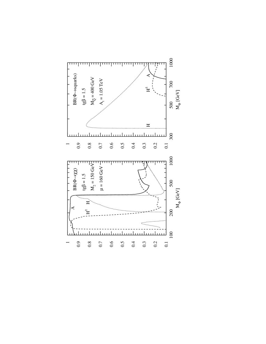
Figure 43: Branching ratios of the MSSM Higgs boson $H,A,H^{\pm}$ decays into charginos/neutralinos and squarks as a function of their masses for $\mbox{tg$\beta$}=1.5$. The mixing parameters have been chosen as $\mu=160$ GeV, $A_{t}=1.05$ TeV, $A_{b}=0$ and the squark masses of the first two generations as $M_{\widetilde{Q}}=400$ GeV. The gaugino mass parameter has been set to $M_{2}=150$ GeV.

Decays into sleptons and squarks.

The sfermionic decay widths of the MSSM Higgs bosons $H_{k}$ [$k=1,2,3,4$ correspond to $H,h,A,H^{\pm}$ and $i,j=1,2$] can be written as [109]

$$\Gamma(H_{k}\to\tilde{f}_{i}\overline{\tilde{f}}_{j})=\frac{3G_{F}}{2\sqrt{2}\pi M_{H_{k}}}\sqrt{\lambda_{\tilde{f}_{i}\tilde{f}_{j},H_{k}}}(g^{H_{k}}_{\tilde{f}_{i}\tilde{f}_{j}})^{2}\,.$$ (156)

The physical MSSM couplings $g^{H_{k}}_{\tilde{f}_{i}\tilde{f}_{j}}$ can be obtained from the couplings presented in eqs. (151) and (152) by means of the mixing relations in eq. (147). The symbol $\lambda_{ij,k}$ denotes the usual two-body phase-space factor of eq. (154).

In the limit of massless fermions, which is a valid approximation for the first two generations, the pseudoscalar Higgs bosons $A$ do not decay into sfermions due to the suppression of sfermion mixing by the fermion mass. In the decoupling regime, where the Higgs masses $M_{H,H^{\pm}}$ are large, the decay widths of the heavy scalar and charged Higgs particles into sfermions are proportional to [109]

$$\Gamma(H,H^{\pm}\to\tilde{f}\overline{\tilde{f}})\propto\frac{G_{F}M_{W}^{4}}{M_{H,H^{\pm}}}\sin^{2}2\beta\,.$$ (157)

Thus they are only important for small $\mbox{tg$\beta$}\sim 1$. However, they are suppressed by an inverse power of the large Higgs masses, rendering unimportant the sfermion decays of the first two generations.

Decay widths into third-generation sfermions [$\tilde{t},\tilde{b},\tilde{\tau}$] can be much larger, thanks to the significantly larger fermion masses. For instance, in the asymptotic regime the heavy scalar Higgs decay into stop pairs of the same helicity is proportional to [109]

$$\Gamma(H\to\tilde{t}\overline{\tilde{t}})\propto\frac{G_{F}M_{t}^{4}}{M_{H}\mbox{tg${}^{2}\beta$}}\,,$$ (158)

which will be enhanced by large coefficients compared to the first/second-generation squarks for small tg$\beta$. At large tg$\beta$ sbottom decays will be significant. Moreover, for large Higgs masses the decay widths of heavy neutral CP-even and CP-odd Higgs particles into stop pairs of different helicity will be proportional to [109]

$$\Gamma(H,A\to\tilde{t}\overline{\tilde{t}})\propto\frac{G_{F}M_{t}^{2}}{M_{H,A}}\left[\mu+\frac{A_{t}}{\mbox{tg$\beta$}}\right]^{2}$$ (159)

and hence will be of the same order of magnitude as standard fermion and chargino/neutralino decay widths. In summary, if third-generation sfermion decays are kinematically allowed, they have to be taken into account. An extreme example for the total branching ratios of decays into squarks is depicted in Fig. 43, where they can reach values of $\sim 80\%$ for the heavy scalar Higgs boson $H$.

Very recently the SUSY-QCD corrections to the stop and sbottom decays of the MSSM Higgs bosons have been calculated [111]. They reach about 30%, especially in the threshold regions. They are not included in the present analysis.

3.2 Neutral Higgs Boson Production at the LHC

3.2.1 Gluon fusion: $gg\to\Phi~{}~{}[\Phi=h,H,A]$

The gluon-fusion mechanism [15]

$$pp\to gg\to\Phi$$

dominates the neutral Higgs boson production at the LHC in the phenomenologically relevant Higgs mass ranges for small and moderate values of tg$\beta$. Only for large tg$\beta$ can the associated $\Phi b\bar{b}$ production channel develop a larger cross section due to the enhanced Higgs couplings to bottom quarks [18, 112]. Analogous to the gluonic decay modes, the gluon coupling to the neutral Higgs bosons in the MSSM is built up by loops involving top and bottom quarks as well as squarks, see Fig. 44.

Figure 44: Typical diagram contributing to $gg\to\Phi$ at lowest order.

The partonic cross sections can be obtained from the gluonic widths of the Higgs bosons at lowest order [53, 99]:

$$\hat{\sigma}^{\Phi}_{LO}(gg\to\Phi) = \sigma^{\Phi}_{0}\delta(1-z)$$ (160)

$$\sigma^{\Phi}_{0} = \frac{\pi^{2}}{8M_{\Phi}^{3}}\Gamma_{LO}(\Phi\to gg)$$

$$\sigma^{h/H}_{0} = \frac{G_{F}\alpha_{s}^{2}(\mu)}{288\sqrt{2}\pi}\ \left|\sum_{Q}g_{Q}^{h/H}A_{Q}^{h/H}(\tau_{Q})+\sum_{\widetilde{Q}}g_{\widetilde{Q}}^{h/H}A_{\widetilde{Q}}^{h/H}(\tau_{\widetilde{Q}})\right|^{2}$$

$$\sigma^{A}_{0} = \frac{G_{F}\alpha_{s}^{2}(\mu)}{128\sqrt{2}\pi}\ \left|\sum_{Q}g_{Q}^{A}A_{Q}^{A}(\tau_{Q})\right|^{2}$$

where the scaling variables are defined as $z=M_{\Phi}^{2}/\hat{s}$, $\tau_{i}=4M_{i}^{2}/M_{\Phi}^{2}~{}~{}(i=Q,\widetilde{Q})$, and $\hat{s}$ denotes the partonic c.m. energy squared. The amplitudes $A_{Q,\widetilde{Q}}^{\Phi}(\tau_{Q,\widetilde{Q}})$ are defined in eqs. (104), (108), and the MSSM couplings $g_{Q}^{\Phi},g^{\Phi}_{\widetilde{Q}}$ can be found in Tables 1 and 4. In the narrow-width approximation the hadronic cross sections are given by

$$\sigma_{LO}(pp\to\Phi)=\sigma^{\Phi}_{0}\tau_{\Phi}\frac{d{\cal L}^{gg}}{d\tau_{\Phi}}$$ (161)

with the gluon luminosity defined in eq. (59) and the scaling variables $\tau_{\Phi}=M^{2}_{\Phi}/s$ where $s$ specifies the total hadronic c.m. energy squared. For small tg$\beta$ the top loop contribution is dominant, while for large values of tg$\beta$ the bottom quark contribution is strongly enhanced. If the squark masses are less than $\sim 400$ GeV, their contribution is significant, and for squark masses beyond $\sim 500$ GeV they can safely be neglected [99]. This is demonstrated in Fig. 45, where the ratio of the cross section with and without the squark contribution is presented as a function of the corresponding scalar Higgs mass. In the phenomenological mass range the squark loops may enhance the cross section by up to a factor 2.

Figure 45: Ratio of the QCD-corrected cross section $\sigma(pp\to h+X)$ with and without squark loops as a function of the common squark mass $M_{\widetilde{Q}}$ for two values of $\mbox{tg$\beta$}=1.5,30$, and for $M_{A}=100$ GeV. The secondary axes present the corresponding light scalar Higgs mass $M_{h}$. The top and bottom masses have been chosen as $M_{t}=175$ GeV, $M_{b}=5$ GeV, and the cross sections are convoluted with CTEQ4M parton densities using $\alpha_{s}(M_{Z})=0.116$ as the normalization of the NLO strong coupling constant.

QCD corrections.

In the past the two-loop QCD corrections to the gluon-fusion cross section were calculated [53, 103]. In complete analogy to the SM case they consist of virtual corrections to the basic $gg\to\Phi$ process and real corrections due to the associated production of the Higgs bosons with massless partons,

$$gg\rightarrow\Phi g\hskip 14.22636pt\mbox{and}\hskip 14.22636ptgq\rightarrow\Phi q,~{}q\overline{q}\rightarrow\Phi g\,.$$

Thus the contributions to the final result for the hadronic cross section can be classified as

$$\sigma(pp\rightarrow\Phi+X)=\sigma^{\Phi}_{0}\left[1+C^{\Phi}\frac{\alpha_{s}}{\pi}\right]\tau_{\Phi}\frac{d{\cal L}^{gg}}{d\tau_{\Phi}}+\Delta\sigma^{\Phi}_{gg}+\Delta\sigma^{\Phi}_{gq}+\Delta\sigma^{\Phi}_{q\bar{q}}\,.$$ (162)

The analytic expressions for arbitrary Higgs boson and quark masses are rather involved and can be found in [53]. As in the SM case the (s)quark-loop masses have been identified with the pole masses $M_{Q}\,(M_{\widetilde{Q}})$, while the QCD coupling is defined in the $\overline{\rm MS}$ scheme. We have adopted the $\overline{\rm MS}$ factorization scheme for the NLO parton densities. The axial $\gamma_{5}$ coupling has been regularized in the ’t Hooft–Veltman scheme [102], which preserves the chiral symmetry in the massless quark limit and fulfills the non-renormalization theorem of the ABJ anomaly at vanishing momentum transfer [105].

The coefficients $C^{\Phi}(\tau_{Q},\tau_{\widetilde{Q}})$ split into the infrared $\pi^{2}$ term, a logarithmic term including the renormalization scale $\mu$, and finite (s)quark mass-dependent pieces $c^{\Phi}(\tau_{Q},\tau_{\widetilde{Q}})$:

$$C^{\Phi}(\tau_{Q},\tau_{\widetilde{Q}})=\pi^{2}+c^{\Phi}(\tau_{Q},\tau_{\widetilde{Q}})+\frac{33-2N_{F}}{6}\log\frac{\mu^{2}}{M_{\Phi}^{2}}\,.$$ (163)

The terms $c^{\Phi}(\tau_{Q})$ originating from quark loops have been reduced analytically to one-dimensional Feynman-parameter integrals, which were evaluated numerically [53, 103]. The QCD corrections to the squark contributions are only known in the heavy-squark limit [99], which however provides a reasonable approximation to the $K$ factor due to the dominance of soft and collinear gluon radiation for heavy particle loops in the gluon-fusion process.

The remaining contributions of eq. (162) can be cast into the form [53, 103]

$$\Delta\sigma^{\Phi}_{gg} = \int_{\tau_{\Phi}}^{1}d\tau\frac{d{\cal L}^{gg}}{d\tau}\times\frac{\alpha_{s}}{\pi}\sigma^{\Phi}_{0}\left\{-zP_{gg}(z)\log\frac{M^{2}}{\hat{s}}+d^{\Phi}_{gg}(z,\tau_{Q},\tau_{\widetilde{Q}})\right.$$

$$\left.\hskip 105.2751pt+12\left[\left(\frac{\log(1-z)}{1-z}\right)_{+}-z[2-z(1-z)]\log(1-z)\right]\right\}$$

$$\Delta\sigma^{\Phi}_{gq} = \int_{\tau_{\Phi}}^{1}d\tau\sum_{q,\bar{q}}\frac{d{\cal L}^{gq}}{d\tau}\times\frac{\alpha_{s}}{\pi}\sigma^{\Phi}_{0}\left\{-\frac{z}{2}P_{gq}(z)\log\frac{M^{2}}{\hat{s}(1-z)^{2}}+d^{\Phi}_{gq}(z,\tau_{Q},\tau_{\widetilde{Q}})\right\}$$

$$\Delta\sigma^{\Phi}_{q\bar{q}} = \int_{\tau_{\Phi}}^{1}d\tau\sum_{q}\frac{d{\cal L}^{q\bar{q}}}{d\tau}\times\frac{\alpha_{s}}{\pi}\sigma^{\Phi}_{0}~{}d^{\Phi}_{q\bar{q}}(z,\tau_{Q},\tau_{\widetilde{Q}})\,,$$ (164)

with $z=\tau_{\Phi}/\tau=M_{\Phi}^{2}/\hat{s}$. $P_{gg}$ and $P_{gq}$ are the standard Altarelli–Parisi splitting functions defined in eq. (63). The coefficients $d^{\Phi}_{gg},d^{\Phi}_{gq}$ and $d^{\Phi}_{q\overline{q}}$ have been reduced to one-dimensional integrals for the quark loops, which can be evaluated numerically [53, 103] for arbitrary quark masses. They can be calculated analytically in the heavy- and light-quark limits.

In the heavy-quark limit the quark contributions to the coefficients $c^{\Phi}(\tau_{Q})$ and $d^{\Phi}_{ij}(z,\tau_{Q})$ reduce to the same expressions as in the SM case of eq. (64) for the scalar Higgs particles $h,H$. For the pseudoscalar Higgs boson only the coefficient $c^{A}(\tau_{Q})$ differs from the scalar case,

$$\tau_{Q}=4M_{Q}^{2}/M_{A}^{2}\gg 1\,:\hskip 85.35826ptc^{A}(\tau_{Q})\to 6\,.\hskip 156.49014pt$$ (165)

In fact, the leading terms in the heavy-quark limit provide a reliable approximation for small tg$\beta$ up to Higgs masses of $\sim 1$ TeV as can be inferred from Fig. 46, which shows the exact pseudoscalar cross sections (solid lines) as a function of the pseudoscalar Higgs mass for three values of tg$\beta$ and the approximation obtained by multiplying the full massive leading-order cross section with the $K$ factor obtained in the heavy-quark limit. A maximal deviation $\sim 25\%$ for $\mbox{tg$\beta$}\raisebox{-3.69899pt}{~{}\shortstack{$<$ \\ [-0.07cm] $\sim$}}~{}5$ occurs in the intermediate mass range.

Figure 46: Comparison of the exact and approximate NLO cross section $\sigma(pp\to A+X)$ at the LHC with c.m. energy $\sqrt{s}=14$ TeV. The solid lines show the exact cross sections including the full $t,b$ quark mass dependence and the dashed lines correspond to the heavy-quark approximation of the K factor. The renormalization and factorization scales have been identified with the Higgs mass, $\mu=M=M_{A}$ and the CTEQ4M parton densities with NLO strong coupling [$\alpha_{s}(M_{Z})=0.116$] have been adopted. The top mass has been chosen as $M_{t}=175$ GeV, the bottom mass as $M_{b}=5$ GeV and the common squark mass as $M_{S}=1$ TeV.

The squark contribution in the heavy-squark limit coincides with the heavy-quark case apart from the virtual piece [99],

$$\tau_{\widetilde{Q}}=4M_{\widetilde{Q}}^{2}/M_{h/H}^{2}\gg 1\,:\hskip 85.35826ptc^{h/H}(\tau_{\widetilde{Q}})\to\frac{25}{3}\,.\hskip 128.0374pt$$ (166)

The QCD corrections to the squark loops have been evaluated for degenerate squark masses, so that no mixing effects occur, and for heavy gluinos, such that their contributions are suppressed. In this case there are no squark loop effects in pseudoscalar Higgs production.

In the opposite limit, where the Higgs mass is much larger than the quark mass, the analytic results coincide with the SM expressions for both the scalar and pseudoscalar Higgs particles [53]. This coincidence reflects the restoration of the chiral symmetry in the massless quark limit.

Figure 47: K factors of the QCD-corrected gluon-fusion cross section $\sigma(pp\to\Phi+X)$ at the LHC with c.m. energy $\sqrt{s}=14$ TeV. The dashed lines show the individual contributions of the four terms of the QCD corrections given in eq. (162). The renormalization and factorization scales have been identified with the corresponding Higgs mass, $\mu=M=M_{\Phi}$, and the CTEQ4M parton densities have been adopted.

The $K$ factors $K_{tot}=\sigma_{NLO}/\sigma_{LO}$ are presented for LHC energies in Fig. 47 as a function of the corresponding Higgs boson mass. Both the renormalization and the factorization scales have been identified with the Higgs masses $\mu=M=M_{\Phi}$. The variation of the $K$ factors with the Higgs masses is mainly caused by the MSSM couplings apart from the threshold region, where in the pseudoscalar case a Coulomb singularity emerges in analogy to the gluonic and photonic decay modes [53, 103]. The corrections are positive and large, increasing the MSSM Higgs production cross sections at the LHC by up to about 100%.

Figure 48: K factors of the cross sections $\sigma(pp\to h/H+X)$ with [solid lines] and without [dashed lines] squark loops as a function of the corresponding scalar Higgs mass for two values of $\mbox{tg$\beta$}=1.5,30$. The common squark mass has been chosen as $M_{\widetilde{Q}}=200$ GeV. The top and bottom masses have been set to $M_{t}=175$ GeV, $M_{b}=5$ GeV, and the NLO cross sections are convoluted with CTEQ4M parton densities using $\alpha_{s}(M_{Z})=0.116$ as the normalization of the NLO strong coupling constant. The LO cross sections are evaluated with CTEQ4L parton densities with the LO strong coupling $\alpha_{s}(M_{Z})=0.132$.

The effect of the squark loops on the scalar Higgs $K$ factors is presented in Fig. 48, which shows the $K$ factors of scalar Higgs boson production with and without squark loops as a function of the corresponding Higgs mass. It is clearly visible that the squark loops hardly change the $K$ factors, making the $K$ factors from the pure quark contributions an excellent approximation within maximal deviations of about 10%.

Theoretical uncertainties in the prediction of the Higgs cross section originate from two sources, the dependence of the cross section on different parametrizations of the parton densities and the unknown NNLO corrections. For representative sets of recent parton distributions [87, 88], we find a variation of about $\pm 10\%$ of the cross section for Higgs masses larger than $\sim 100$ GeV analogous to the SM case. The uncertainty due to the gluon density will be smaller in the near future when the deep-inelastic electron/positron–nucleon scattering experiments at HERA will have reached the anticipated level of accuracy.

Figure 49: The renormalization and factorization scale dependence of the Higgs production cross section at lowest and next-to-leading order for two different Higgs bosons $H,A$ with masses $M_{H}=500$ GeV and $M_{A}=100$ GeV and two values of $\mbox{tg$\beta$}=1.5,30$.

The [unphysical] variation of the cross sections with the renormalization and factorization scales is reduced by including the NLO corrections. This is shown in Fig. 49 for the heavy scalar and pseudoscalar Higgs particles with masses $M_{H}=500$ GeV and $M_{A}=100$ GeV. The renormalization/factorization scale $\mu=M$ is varied in units of the Higgs mass $\mu=\xi M_{\Phi}$. The remaining uncertainties due to the scale dependence appear to be less than about 15%.

Soft gluon resummation.

Recently soft and collinear gluon radiation effects for the total gluon-fusion cross section have been resummed [91]. In complete analogy to the SM case, the perturbative expansion of the resummed result leads to a quantitative approximation of the three-loop NNLO corrections of the partonic cross section in the heavy top mass limit, which approximates the full massive NLO result with a reliable precision for small and medium values of tg$\beta$ [see Fig. 46]. Owing to the low-energy theorems discussed before [see the gluonic decay modes $\Phi\to gg$], the unrenormalized partonic cross section factorizes in the same way as the SM cross section. The scalar factors $\kappa^{h/H}$ coincide with the SM values of eq. (68) and the pseudoscalar factor is equal to unity, because of the non-renormalization of the ABJ anomaly [105],

$$\kappa^{A}=1\,.$$ (167)

The resummation of soft and collinear gluon effects proceeds along the same lines as in the SM case. The final results for the scalar correction factors $\rho^{h/H}$ are identical to the SM result eq. (78), and the pseudoscalar correction factor can be cast into the form [91]

$$\rho^{A}\left(N,\frac{M_{A}^{2}}{\mu^{2}},\alpha_{s}(\mu)\right)=\rho^{h/H}\left(N,\frac{M_{A}^{2}}{\mu^{2}},\alpha_{s}(\mu)\right)\times\exp\left\{6\frac{\alpha_{s}(M_{A}^{2})}{\pi}\right\}\,.$$ (168)

The perturbative expansions at NLO and NNLO [91] read as [for $\mu=M$]

$$\rho_{A}^{(1)}\left(z,\frac{M_{A}^{2}}{\mu^{2}}\right) = \rho_{h/H}^{(1)}\left(z,\frac{M_{A}^{2}}{\mu^{2}}\right)+6\delta(1-z)$$ (169)

$$\rho_{A}^{(2)}\left(z,\frac{M_{A}^{2}}{\mu^{2}}\right) = \rho_{h/H}^{(2)}\left(z,\frac{M_{A}^{2}}{\mu^{2}}\right)+3\left\{24{\cal D}_{1}(z)-12L_{\mu}{\cal D}_{0}(z)-48{\cal E}_{1}(z)\right.$$ (170)

$$\left.+(12\zeta_{2}+6+\beta_{0}L_{\mu})\delta(1-z)\right\}$$

where we use the same notation as in the SM case.

Figure 50: Exact and approximate two- and three-loop correction factor convoluted with NLO gluon densities in the heavy top quark limit for the pseudoscalar MSSM Higgs boson. The CTEQ4M parton densities have been adopted with $\alpha_{s}(M_{Z})=0.116$ at NLO.

The convolution of the scalar correction factors with NLO gluon densities and strong coupling coincides with the SM case in Fig. 24, while the pseudoscalar case is presented in Fig. 50 as a function of the pseudoscalar Higgs mass at the LHC. The solid line corresponds to the exact NLO result and the lower dashed line to the NLO expansion of the resummed correction factor. It can be inferred from this figure that the soft gluon approximation reproduces the exact result within $\sim 5\%$ at NLO. The upper dashed line shows the NNLO expansion of the resummed correction factor. Fig. 50 demonstrates that the correction factor amounts to about 2.2–2.5 at NLO and 3.2–4.1 at NNLO in the phenomenologically relevant Higgs mass range $M_{A}\raisebox{-3.69899pt}{~{}\shortstack{$<$ \\ [-0.07cm] $\sim$}}~{}1$ TeV. However, in order to evaluate the size of the QCD corrections, each order of the perturbative expansion has to be integrated with the strong coupling and parton densities of the same order, i.e. LO cross section with LO quantities, NLO cross section with NLO quantities and NNLO cross section with NNLO quantities. This consistent $K$ factor amounts to about 1.5–2.0 at NLO and is thus about 50–60% smaller than the result in Fig. 50. A reliable prediction of the gluon-fusion cross section at NNLO requires the convolution with NNLO parton densities, which are not yet available. It is thus impossible to predict the Higgs production cross sections with NNLO accuracy until NNLO structure functions are accessible.

The scale dependence at NNLO develops a similar picture as in the SM case. For large Higgs masses a broad maximum appears near the natural scale $\mu=M=M_{\Phi}$ indicating an important theoretical improvement in the prediction of the Higgs production cross section [91].

3.2.2 Vector boson fusion: $qq\to qqV^{*}V^{*}\to qqh/qqH$

Figure 51: Diagram contributing to $qq\to qqV^{*}V^{*}\to qqh/qqH$ at lowest order.

Due to the absence of vector boson couplings to pseudoscalar Higgs particles $A$, only the scalar Higgs bosons $h,H$ can be produced via the vector-boson-fusion mechanism at tree level [see Fig. 51]. However, these processes are suppressed with respect to the SM cross section due to the MSSM couplings [$g_{V}^{h/H}=\sin(\alpha-\beta)/\cos(\alpha-\beta)$],

$$\sigma(pp\to qq\to qqh/qqH)=\left(g_{V}^{h/H}\right)^{2}\sigma(pp\to qq\to qqH_{SM})\,.$$ (171)

It turns out that the vector-boson-fusion mechanism is unimportant in the MSSM, because for large heavy scalar Higgs masses $M_{H}$, the MSSM couplings $g_{V}^{H}$ are very small. The relative QCD corrections are the same as for the SM Higgs particle [Fig. 27] and thus small [17].

3.2.3 Higgs-strahlung: $q\bar{q}\to V^{*}\to Vh/VH$

Figure 52: Diagram contributing to $q\bar{q}\to V^{*}\to Vh/VH$ at lowest order.

For the same reasons as in the vector-boson-fusion mechanism case, the Higgs-strahlung off $W,Z$ bosons, $q\bar{q}\to V^{*}\to Vh/VH~{}(V=W,Z)$ [see Fig. 52], is unimportant for the scalar MSSM Higgs particles $h,H$. The cross sections can be easily related to the SM cross sections,

$$\sigma(pp\to Vh/VH)=\left(g_{V}^{h/H}\right)^{2}\sigma(pp\to VH_{SM})\,.$$ (172)

Pseudoscalar couplings to intermediate vector bosons are absent so that pseudoscalar Higgs particles cannot be produced at tree level in this channel. The relative QCD corrections are the same as in the SM case, see Fig. 29, and thus of moderate size [20].

3.2.4 Higgs bremsstrahlung off top and bottom quarks

Figure 53: Typical diagrams contributing to $q\bar{q}/gg\to\Phi Q\bar{Q}~{}~{}(Q=t,b)$ at lowest order.

The scalar Higgs cross sections for Higgs bremsstrahlung off heavy quarks $Q$ can simply be related to the SM case:

$$\sigma(pp\to hQ\bar{Q}/HQ\bar{Q})=\left(g_{Q}^{h/H}\right)^{2}\sigma(pp\to H_{SM}Q\bar{Q})$$ (173)

The expressions for the pseudoscalar Higgs boson [112] are similarly involved as the scalar case and will not be presented here.

The top quark coupling to MSSM Higgs bosons is suppressed with respect to the SM for $\mbox{tg$\beta$}>1$. Therefore Higgs bremsstrahlung off top quarks $pp\to\Phi t\bar{t}$ is less important for MSSM Higgs particles. On the other hand Higgs bremsstrahlung off bottom quarks $pp\to Hb\bar{b}$ will be the dominant Higgs production channel for large tg$\beta$ due to the strongly enhanced bottom quark Yukawa couplings [18]. The QCD corrections to $HQ\bar{Q}$ production are still unknown.

3.2.5 Cross sections for Higgs boson production at the LHC

Fig. 54a

Fig. 54b

Figure 54: Neutral MSSM Higgs production cross sections at the LHC [$\sqrt{s}=14$ TeV] for gluon fusion $gg\to\Phi$, vector-boson fusion $qq\to qqVV\to qqh/qqH$, vector-boson bremsstrahlung $q\bar{q}\to V^{*}\to hV/HV$ and the associated production $gg,q\bar{q}\to\Phi b\bar{b}/\Phi t\bar{t}$ including all known QCD corrections. (a) $h,H$ production for $\mbox{tg$\beta$}=1.5$, (b) $h,H$ production for $\mbox{tg$\beta$}=30$, (c) $A$ production for $\mbox{tg$\beta$}=1.5$, (d) $A$ production for $\mbox{tg$\beta$}=30$.

Fig. 54c

Fig. 54d

Figure 54: Continued.

Previous studies of MSSM Higgs boson production at the LHC [113] were based on lowest-order cross sections or included a part of the QCD corrections. We have updated these analyses by including all known QCD corrections to the production processes and the two-loop corrections to the MSSM Higgs sector, thus rendering the results more accurate and reliable than in the previous studies.

The cross sections of the various MSSM Higgs production mechanisms at the LHC are shown in Figs. 54a–d for two representative values of $\mbox{tg$\beta$}=1.5,30$ as a function of the corresponding Higgs mass. The total c.m. energy has been chosen as $\sqrt{s}=14$ TeV, the CTEQ4M parton densities have been adopted with $\alpha_{s}(M_{Z})=0.116$, and the top and bottom masses have been set to $M_{t}=175$ GeV and $M_{b}=5$ GeV. For the Higgs bremsstrahlung off $t,b$ quarks, $pp\to\Phi Q\bar{Q}+X$, we have used the leading order CTEQ4L parton densities, because the NLO QCD corrections are unknown. Thus the consistent evaluation of this cross section requires LO parton densities and strong coupling. The latter is normalized as $\alpha_{s}(M_{Z})=0.132$ at lowest order. For small and moderate values of $\mbox{tg$\beta$}\raisebox{-3.69899pt}{~{}\shortstack{$<$ \\ [-0.07cm] $\sim$}}~{}10$ the gluon-fusion cross section provides the dominant production cross section for the entire Higgs mass region up to $M_{\Phi}\sim 1$ TeV. However, for large tg$\beta$, Higgs bremsstrahlung off bottom quarks, $pp\to\Phi b\bar{b}+X$, dominates over the gluon-fusion mechanism through the strongly enhanced bottom Yukawa couplings.

The MSSM Higgs search at the LHC will be more involved than the SM Higgs search. The basic features can be summarized as follows.

(i) 

For large pseudoscalar Higgs masses $M_{A}\raisebox{-3.69899pt}{~{}\shortstack{$>$ \\ [-0.07cm] $\sim$}}~{}200$ GeV the light scalar Higgs boson $h$ can only be found via its photonic decay mode $h\to\gamma\gamma$. In a significant part of this MSSM parameter region, especially for moderate values of tg$\beta$, no other MSSM Higgs particle can be discovered. Because of the decoupling limit for large $M_{A}$ the MSSM cannot be distinguished from the SM in this mass range.

(ii) 

For small values of $\mbox{tg$\beta$}\raisebox{-3.69899pt}{~{}\shortstack{$<$ \\ [-0.07cm] $\sim$}}~{}3$ and pseudoscalar Higgs masses between about 200 and 350 GeV, the heavy scalar Higgs boson can be searched for in the ‘gold-plated’ channel $H\to ZZ\to 4l^{\pm}$. Otherwise this ‘gold-plated’ signal does not play any rôle in the MSSM. However, the detectable MSSM parameter region hardly exceeds the anticipated exclusion limits of the LEP2 experiments.

(iii)

For large and moderate values of $\mbox{tg$\beta$}\raisebox{-3.69899pt}{~{}\shortstack{$>$ \\ [-0.07cm] $\sim$}}~{}3$ the decays $H,A\to\tau^{+}\tau^{-}$ become visible at the LHC. Thus this decay mode plays a significant rôle for the MSSM in contrast to the SM. Moreover, it will also be detectable for small values of $\mbox{tg$\beta$}\raisebox{-3.69899pt}{~{}\shortstack{$>$ \\ [-0.07cm] $\sim$}}~{}1$–$2$ and $M_{A}\raisebox{-3.69899pt}{~{}\shortstack{$<$ \\ [-0.07cm] $\sim$}}~{}200$ GeV.

(iv)

For $\mbox{tg$\beta$}\raisebox{-3.69899pt}{~{}\shortstack{$<$ \\ [-0.07cm] $\sim$}}~{}4$ and 150 GeV $\!\!\raisebox{-3.69899pt}{~{}\shortstack{$<$ \\ [-0.07cm] $\sim$}}~{}M_{A}\raisebox{-3.69899pt}{~{}\shortstack{$<$ \\ [-0.07cm] $\sim$}}~{}400$ GeV the heavy scalar Higgs particle can be detected via its decay mode $H\to hh\to b\bar{b}\gamma\gamma$. However, the MSSM parameter range for this signature is very limited.

(v) 

For $\mbox{tg$\beta$}\raisebox{-3.69899pt}{~{}\shortstack{$<$ \\ [-0.07cm] $\sim$}}~{}3$–$5$ and 50 GeV $\!\!\raisebox{-3.69899pt}{~{}\shortstack{$<$ \\ [-0.07cm] $\sim$}}~{}M_{A}\raisebox{-3.69899pt}{~{}\shortstack{$<$ \\ [-0.07cm] $\sim$}}~{}350$ GeV the pseudoscalar decay mode $A\to Zh\to l^{+}l^{-}b\bar{b}$ will be visible, but hardly exceeds the exclusion limits from LEP2.

(vi)

For pseudoscalar Higgs masses $M_{A}\raisebox{-3.69899pt}{~{}\shortstack{$<$ \\ [-0.07cm] $\sim$}}~{}100$ GeV charged Higgs bosons, produced from top quark decays $t\to H^{+}b$, can be discovered via its decay mode $H^{+}\to\tau^{+}\bar{\nu}_{\tau}$.

The final picture exhibits a difficult region for the MSSM Higgs search at the LHC. For $\mbox{tg$\beta$}\sim 5$ and $M_{A}\sim 150$ GeV the full luminosity and the full data sample of both the ATLAS and CMS experiments at the LHC, are needed to cover the problematic parameter region [114], see Fig. 55. On the other hand, if no excess of Higgs events above the SM background processes beyond 2 standard deviations will be found, the MSSM Higgs bosons can easily be excluded at 95% C.L.

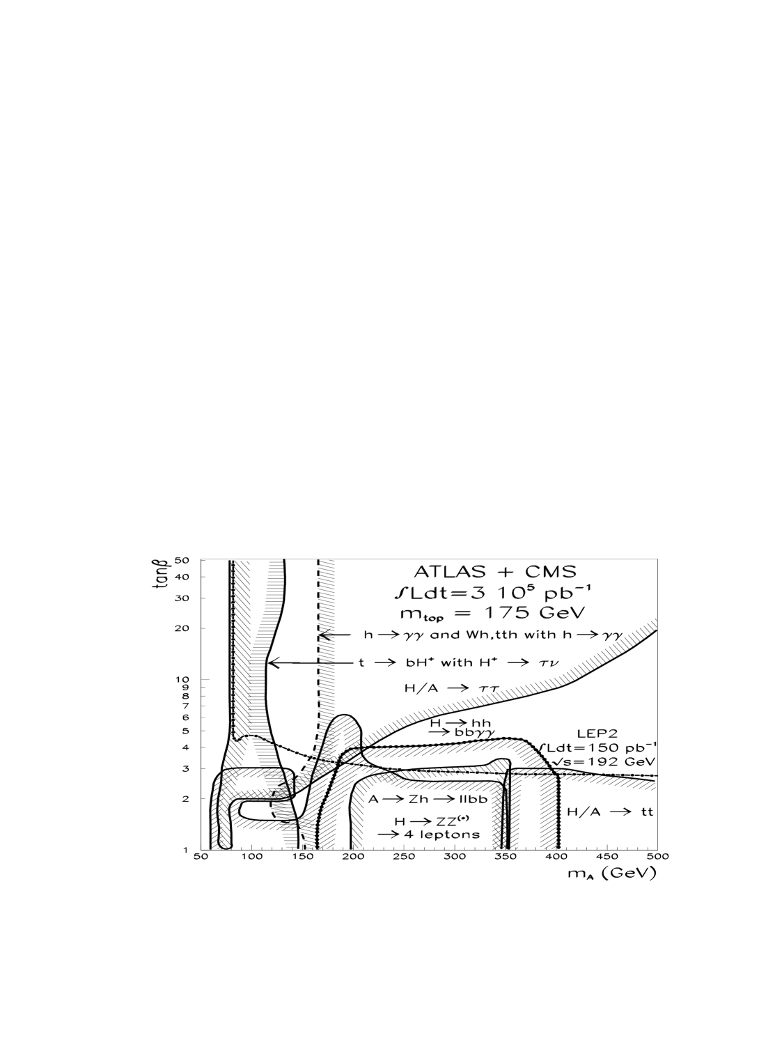
Figure 55: MSSM parameter space including the contours of the various Higgs decay modes, which will be visible at the LHC after reaching the anticipated integrated luminosity $\int{\cal L}dt=3\times 10^{5}\,pb^{-1}$ and combining the experimental data of both LHC experiments, ATLAS and CMS [taken from Ref. [114]].

4 Summary

In this review the decay widths and branching ratios of SM and MSSM Higgs bosons have been updated. All relevant higher order corrections, which are dominated by QCD corrections, have been taken into account. We have thus presented the branching ratios and decay widths of SM and MSSM Higgs particles with the best available theoretical accuracy.

At the LHC the SM Higgs particle will be produced predominantly by gluon fusion $gg\to H$, followed by vector-boson fusion $VV\to H$ ($V=W,Z$) and, to a lesser extent, Higgs-strahlung off vector bosons, $V^{*}\to VH$, and top quarks, $gg/q\bar{q}\to t\bar{t}H$. The cross sections of these production channels have been updated by including all known QCD corrections, which are important in particular for the dominant gluon-fusion mechanism. Thus the final results of this review may serve as a benchmark of the theoretical predictions for SM Higgs boson production at the LHC.

For Higgs masses $M_{H}\raisebox{-3.69899pt}{~{}\shortstack{$>$ \\ [-0.07cm] $\sim$}}~{}140$ GeV the SM Higgs search at the LHC will proceed via the ‘gold-plated’ $H\to ZZ^{(*)}\to 4l^{\pm}$ decay mode with small SM backgrounds. The extraction of four charged lepton signals at the LHC will probe Higgs masses up to about 800 GeV. In the Higgs mass range 155 GeV$\raisebox{-3.69899pt}{~{}\shortstack{$<$ \\ [-0.07cm] $\sim$}}~{}M_{H}\raisebox{-3.69899pt}{~{}\shortstack{$<$ \\ [-0.07cm] $\sim$}}~{}180$ GeV the SM Higgs boson can also easily be found via its decay channel $H\to WW\to l^{+}l^{-}\nu\bar{\nu}$, by means of the specific angular correlations among the charged leptons. Moreover, the decay channel $H\to l^{+}l^{-}\nu\bar{\nu}$ may allow for an extension of the Higgs search up to Higgs masses beyond 1 TeV. For $M_{W}\raisebox{-3.69899pt}{~{}\shortstack{$<$ \\ [-0.07cm] $\sim$}}~{}M_{H}\raisebox{-3.69899pt}{~{}\shortstack{$<$ \\ [-0.07cm] $\sim$}}~{}140$ GeV, the only promising decay mode seems to be provided by the photonic decay $H\to\gamma\gamma$, the detection of which, however, requires excellent energetic and geometric resolutions of the detectors in order to suppress the large QCD backgrounds. Higgs-strahlung off vector bosons or top quarks, with the Higgs decaying into a photon pair, may allow a further reduction of the background, but unfortunately the signal rates are small. In the case of excellent $b$-tagging the dominant $b\bar{b}$ decay mode of the Higgs might be detectable, if the Higgs particle is produced in association with a $W$ boson or $t\bar{t}$ pair.

In the MSSM the neutral Higgs bosons will mainly be produced via gluon fusion $gg\to\Phi$. However, through the enhanced $b$ quark couplings, Higgs bremsstrahlung off $b$ quarks, $gg/q\bar{q}\to b\bar{b}\Phi$, will dominate for large tg$\beta$. All other Higgs production mechanisms, i.e. vector-boson fusion and Higgs-strahlung off vector bosons or $t\bar{t}$ pairs, will be less important than in the SM.

The ‘gold-plated’ $H\to ZZ\to 4l^{\pm}$ signal does not play an important rôle in the MSSM. On the other hand the $\tau$ lepton pair decays $H,A\to\tau^{+}\tau^{-}$ will be visible for large values of tg$\beta$. The light scalar Higgs particle will only be visible via its photonic decay mode $h\to\gamma\gamma$, the branching ratio of which will be smaller than in the SM because of the suppressed SUSY couplings. Moreover, the decay modes $H\to hh\to b\bar{b}\gamma\gamma$, $H/A\to t\bar{t}$ and $A\to Zh\to l^{+}l^{-}b\bar{b}$ will be detectable in very restricted regions of the MSSM parameter space. Finally charged Higgs particles may be looked for in the top quark decays $t\to H^{+}b$ at the lower end of the charged Higgs mass range. In the search for the MSSM Higgs particles at the LHC, the maximal anticipated integrated luminosity will be needed, especially to cover the difficult region around $M_{A}\sim 150$ GeV and $\mbox{tg$\beta$}\sim 5$.

Acknowledgements
First I would like to thank G. Kramer and P.M. Zerwas for the fruitful collaboration on QCD and Higgs physics. Thanks also go to other collaborators: A. Djouadi, S. Dawson, J. Kalinowski, B. Kniehl, M. Krämer, E. Laenen and D. Graudenz. Moreover, I am grateful to G. Kramer for encouraging me to complete this work. I thank F. Gianotti for providing me with Fig. 32. Finally I am also grateful to P.M. Zerwas, A. Djouadi, S. Dawson and A. Kataev for reading the manuscript and their valuable comments.

References

• [1] P. W. Higgs, Phys. Rev. Lett. 12 (1964) 132 and Phys. Rev. 145 (1966) 1156;
F. Englert and R. Brout, Phys. Rev. Lett. 13 (1964) 321;
G. S. Guralnik, C. R. Hagen and T. W. Kibble, Phys. Rev. Lett. 13 (1964) 585.
• [2] M. Veltman, Nucl. Phys. B7 (1968) 637;
G. ’t Hooft, Nucl. Phys. B33 (1971) 173 and Nucl. Phys. B35 (1971) 167.
• [3] For a review on the Higgs sector in the Standard Model and in its supersymmetric extensions, see J. Gunion, H. Haber, G. Kane and S. Dawson, “The Higgs Hunter’s Guide” (Addison–Wesley, Reading, Mass., 1990).
• [4] N. Cabibbo, L. Maiani, G. Parisi and R. Petronzio, Nucl. Phys. B158 (1979) 295;
M. Chanowitz, M. Furman and I. Hinchliffe, Phys. Lett. B78 (1978) 285;
R.A. Flores and M. Sher, Phys. Rev. D27 (1983) 1679;
M. Lindner, Z. Phys. C31 (1986) 295;
M. Sher, Phys. Rep. 179 (1989) 273; Phys. Lett. B317 (1993) 159 and addendum B331 (1994) 448;
G. Altarelli and G. Isidori, Phys. Lett. B337 (1994) 141;
J. Casas, J. Espinosa and M. Quiros, Phys. Lett. B342 (1995) 171.
• [5] J. Espinosa and M. Quiros, Phys. Lett. B353 (1995) 257.
• [6] A. Hasenfratz, K. Jansen, C. Lang, T. Neuhaus and H. Yoneyama, Phys. Lett. B199 (1987) 531;
J. Kuti, L. Liu and Y. Shen, Phys. Rev. Lett. 61 (1988) 678;
M. Lüscher and P. Weisz, Nucl. Phys. B318 (1989) 705.
• [7] J. Erler and P. Langacker, Phys. Rev. D52 (1995) 441.
• [8] F. Abe et al., CDF Collaboration, Phys. Rev. Lett. 73 (1994) 225;
S. Abachi et al., D0 Collaboration, Phys. Rev. Lett. 79 (1997) 1197.
• [9] P. Janot, Proceedings, Europhysics Conference on High Energy Physics, Jerusalem 1997.
• [10] J. Ellis, M.K. Gaillard and D.V. Nanopoulos, Nucl. Phys. B106 (1976) 292.
• [11] B.L. Ioffe, The XXI Session of the Scientific Coordination Meeting of IHEP, Protvino 1976;
J.D. Bjorken, Proceedings Summer Institute on Particle Physics, Report SLAC-198 (1976);
B.L. Ioffe and V.A. Khoze, Sov. J. Part. Nucl. 9 (1978) 50.
• [12] B.W. Lee, C. Quigg and H.B. Thacker, Phys. Rev. D16 (1977) 1519.
• [13] D. Froidevaux, Z. Kunszt and J. Stirling [conv.] et al. in the Proceedings of the Large Hadron Collider Workshop, Aachen 1990, CERN Report 90–10, Vol. II;
see also the Rapporteurs talks by G. Altarelli and D. Denegri, $ibid.$, Vol. I.
• [14] ATLAS Collaboration, Technical Proposal, Report CERN–LHCC 94–43 (December 1994);
CMS Collaboration, Technical Proposal, Report CERN–LHCC 94–38 (December 1994).
• [15] H. Georgi, S. Glashow, M. Machacek and D.V. Nanopoulos, Phys. Rev. Lett. 40 (1978) 692.
• [16] R.N. Cahn and S. Dawson, Phys. Lett. B136 (1984) 196;
K. Hikasa, Phys. Lett. B164 (1985) 341;
G. Altarelli, B. Mele and F. Pitolli, Nucl. Phys. B287 (1987) 205.
• [17] T. Han, G. Valencia and S. Willenbrock, Phys. Rev. Lett. 69 (1992) 3274.
• [18] Z. Kunszt, Nucl. Phys. B247 (1984) 339;
J.F. Gunion, Phys. Lett. B253 (1991) 269;
W.J. Marciano and F.E. Paige, Phys. Rev. Lett. 66 (1991) 2433.
• [19] S.L. Glashow, D.V. Nanopoulos and A. Yildiz, Phys. Rev. D18 (1978) 1724;
Z. Kunszt, Z. Trocsanyi and W.J. Stirling, Phys. Lett. B271 (1991) 247.
• [20] T. Han and S. Willenbrock, Phys. Lett. B273 (1991) 167.
• [21] J. Dai, J.F. Gunion and R. Vega, Phys. Rev. Lett. 71 (1993) 2699.
• [22] D. Froidevaux and E. Richter-Was, Z. Phys. C67 (1995) 213.
• [23] M. Dittmar and H. Dreiner, Phys. Rev. D55 (1997) 167.
• [24] For reviews on supersymmetric theories, see P. Fayet and S. Ferrara, Phys. Rep. 32 (1977) 249;
H.P. Nilles, Phys. Rep. 110 (1984) 1;
R. Barbieri, Riv. Nuovo Cimento 11 (1988) 1.
• [25] H. Haber and G. Kane, Phys. Rep. 117 (1985) 75.
• [26] E. Witten, Phys. Lett. B105 (1981) 267.
• [27] S. Dimopoulos, S. Raby and F. Wilczek, Phys. Rev. D24 (1981) 1681;
L.E. Ibáñez and G.G. Ross, Phys. Lett. B105 (1981) 439.
• [28] H. Haber and M. Sher, Phys. Rev. D35 (1987) 2206;
J.L. Hewett and T.G. Rizzo, Phys. Rep. 183 (1989) 194;
J. Ellis, J.F. Gunion, H. Haber, L. Roszkowski and F. Zwirner, Phys. Rev. D39 (1989) 844;
M. Drees, Int. J. Mod. Phys. A4 (1989) 3635;
T. Elliot, S. King and P. White, Phys. Lett. B305 (1993) 71;
G. Kane, C. Kolda and J. Wells, Phys. Rev. Lett. 70 (1993) 2686;
U. Ellwanger, M. Rausch de Traubenberg and C. Savoy, Z. Phys. C67 (1995) 665.
• [29] S. Dimopoulos and H. Georgi, Nucl. Phys. B193 (1981) 150;
N. Sakai, Z. Phys. C11 (1981) 153;
K. Inoue, A. Komatsu and S. Takeshita, Prog. Theor. Phys. 67 (1982) 927; (E) 70 (1983) 330; 71 (1984) 413;
E. Witten, Nucl. Phys. B231 (1984) 419.
• [30] J. Gunion and A. Turski, Phys. Rev. D39 (1989) 2701 and D40 (1990) 2333;
M. Berger, Phys. Rev. D41 (1990) 225;
Y. Okada, M. Yamaguchi and T. Yanagida, Prog. Theor. Phys. 85 (1991) 1;
H. Haber and R. Hempfling, Phys. Rev. Lett. 66 (1991) 1815;
J. Ellis, G. Ridolfi and F. Zwirner, Phys. Lett. B257 (1991) 83;
R. Barbieri, F. Caravaglios and M. Frigeni, Phys. Lett. B258 (1991) 167;
A. Yamada, Phys. Lett. B263 (1991) 233;
A. Brignole, J. Ellis, G. Ridolfi and F. Zwirner, Phys. Lett. B271 (1991) 123;
P.H. Chankowski, S. Pokorski and J. Rosiek, Phys. Lett. B274 (1992) 191;
M. Drees and M.M. Nojiri, Phys. Rev. D45 (1992) 2482.
• [31] J.R. Espinosa and M. Quiros, Phys. Lett. B266 (1991) 389;
R. Hempfling and A. Hoang, Phys. Lett. B331 (1994) 99;
J.A. Casas, J. Espinosa, M. Quiros and A. Riotto, Nucl. Phys. B436 (1995) 3; (E) B439 (1995) 466;
M. Carena, J. Espinosa, M. Quiros and C.E.M. Wagner, Phys. Lett. B355 (1995) 209;
M. Carena, M. Quiros and C.E.M. Wagner, Nucl. Phys. B461 (1996) 407.
• [32] A. Djouadi, J. Kalinowski and P.M. Zerwas, Z. Phys. C57 (1993) 565.
• [33] A. Djouadi, Int. J. Mod. Phys. A10 (1995) 1.
• [34] B.A. Kniehl, Phys. Rep. 240 (1994) 211.
• [35] A. Djouadi, J. Kalinowski and M. Spira, report CERN–TH/97-254, hep-ph/9704448.
• [36] For a recent update of the effect of QCD corrections to the hadronic decay widths, see A. Djouadi, M. Spira and P.M. Zerwas, Z. Phys. C70 (1996) 427.
• [37] L. Resnick, M.K. Sundaresan and P.J.S. Watson, Phys. Rev. D8 (1973) 172.
• [38] E. Braaten and J.P. Leveille, Phys. Rev. D22 (1980) 715;
N. Sakai, Phys. Rev. D22 (1980) 2220;
T. Inami and T. Kubota, Nucl. Phys. B179 (1981) 171;
S.G. Gorishny, A.L. Kataev and S.A. Larin, Sov. J. Nucl. Phys. 40 (1984) 329;
M. Drees and K. Hikasa, Phys. Rev. D41 (1990) 1547; Phys. Lett. B240 (1990) 455 and (E) B262 (1991) 497.
• [39] S.G. Gorishny, A.L. Kataev, S.A. Larin and L.R. Surguladze, Mod. Phys. Lett. A5 (1990) 2703; Phys. Rev. D43 (1991) 1633;
A.L. Kataev and V.T. Kim, Mod. Phys. Lett. A9 (1994) 1309;
L.R. Surguladze, Phys. Lett. 341 (1994) 61;
K.G. Chetyrkin, J.H. Kühn and A. Kwiatkowski, Proceedings of the Workshop “QCD at LEP”, Aachen, 1994;
K.G. Chetyrkin, Phys. Lett. B390 (1997) 309.
• [40] K.G. Chetyrkin and A. Kwiatkowski, Nucl. Phys. B461 (1996) 3;
S.A. Larin, T. van Ritbergen and J.A.M. Vermaseren, Phys. Lett. B362 (1995) 134.
• [41] K. Melnikov, Phys. Rev. D53 (1996) 5020.
• [42] N. Gray, D.J. Broadhurst, W. Grafe and K. Schilcher, Z. Phys. C48 (1990) 673.
• [43] S. Narison, Phys. Lett. B341 (1994) 73.
• [44] S.G. Gorishny, A.L. Kataev, S.A. Larin and L.R. Surguladze, Mod. Phys. Lett. A5 (1990) 2703; Phys. Rev. D43 (1991) 1633.
• [45] K.G. Chetyrkin, Phys. Lett. B404 (1997) 161;
J.A.M. Vermaseren, S.A. Larin and T. van Ritbergen, Phys. Lett. B405 (1997) 327.
• [46] J. Fleischer and F. Jegerlehner, Phys. Rev. D23 (1981) 2001.
• [47] D.Yu. Bardin, B.M. Vilenskiĭ and P.Kh. Khristova, Sov. J. Nucl. Phys. 53 (1991) 152;
A. Dabelstein and W. Hollik, Z. Phys. C53 (1992) 507;
B.A. Kniehl, Nucl. Phys. B376 (1992) 3.
• [48] A. Djouadi, D. Haidt, B.A. Kniehl, B. Mele and P.M. Zerwas, Proceedings Workshop on $e^{+}e^{-}$ Collisions at 500 GeV: The Physics Potential, ed. P.M. Zerwas, Report DESY 92-123A.
• [49] B.A. Kniehl and M. Spira, Nucl. Phys. B432 (1994) 39;
A. Kwiatkowski and M. Steinhauser, Phys. Lett. B338 (1994) 66 and (E) B342 (1995) 455.
• [50] K.G. Chetyrkin, B.A. Kniehl and M. Steinhauser, Phys. Rev. Lett. 78 (1997) 594.
• [51] A. Ghinculov, Phys. Lett.  B337 (1994) 137 and (E) 346 (1995) 426;
L. Durand, B.A. Kniehl, and K. Riesselmann, Phys. Rev. Lett. 72 (1994) 2534 and (E) 74 (1995) 1699; Phys. Rev. D51 (1995) 5007;
V. Borodulin and G. Jikia, Phys. Lett. B391 (1997) 434.
• [52] A. Djouadi, J. Kalinowski and P.M. Zerwas, Z. Phys. C70 (1996) 437;
S. Moretti and W.J. Stirling, Phys. Lett. B347 (1995) 291 and (E) B366 (1996) 451.
• [53] M. Spira, A. Djouadi, D. Graudenz and P.M. Zerwas, Nucl. Phys. B453 (1995) 17.
• [54] T. Inami, T. Kubota and Y. Okada, Z. Phys. C18 (1983) 69.
• [55] A. Djouadi, M. Spira and P.M. Zerwas, Phys. Lett. B264 (1991) 440.
• [56] K.G. Chetyrkin, B.A. Kniehl and M. Steinhauser, Phys. Rev. Lett. 79 (1997) 353.
• [57] A.I. Vainshtein, M.B. Voloshin, V.I. Zakharov and M.A. Shifman, Sov. J. Nucl. Phys. 30 (1979) 711.
• [58] B.A. Kniehl and M. Spira, Z. Phys. C69 (1995) 77.
• [59] S. Dawson, Nucl. Phys. B359 (1991) 283.
• [60] O. Tarasov, Preprint JINR P2-82-900 (1982), unpublished.
• [61] O. Tarasov, A. Vladimirov and A. Zharkov, Phys. Lett. B93 (1980) 429;
S.A. Larin and J.A.M. Vermaseren, Phys. Lett. B303 (1993) 334.
• [62] T. van Ritbergen, J.A.M. Vermaseren and S.A. Larin, report NIKHEF-97-001, hep-ph/9701390.
• [63] W. Bernreuther and W. Wetzel, Nucl. Phys. B197 (1982) 228;
W. Bernreuther, Ann. Phys. 151 (1983) 127.
• [64] S.A. Larin, T. van Ritbergen and J.A.M. Vermaseren, Nucl. Phys. B438 (1995) 278.
• [65] W. Bernreuther, K.G. Chetyrkin and S.A. Larin, private communication.
• [66] A. Djouadi, Nuovo Cimento A100 (1988) 357;
A. Djouadi and P. Gambino, Phys. Rev. D49 (1994) 3499.
• [67] A. Djouadi and P. Gambino, Phys. Rev. Lett. 73 (1994) 2528;
K.G. Chetyrkin, B.A. Kniehl and M. Steinhauser, Phys. Rev. Lett. 78 (1997) 594 and Nucl. Phys. B490 (1997) 19.
• [68] T. Kinoshita, J. Math. Phys. 3 (1962) 650;
T.D. Lee and M. Nauenberg, Phys. Rev. 133 (1964) 1549.
• [69] H. Zheng and D. Wu, Phys. Rev. D42 (1990) 3760;
A. Djouadi, M. Spira, J. van der Bij and P.M. Zerwas, Phys. Lett. B257 (1991) 187;
S. Dawson and R.P. Kauffman, Phys. Rev. D47 (1993) 1264;
A. Djouadi, M. Spira and P.M. Zerwas, Phys. Lett. B311 (1993) 255;
K. Melnikov and O. Yakovlev, Phys. Lett. B312 (1993) 179;
M. Inoue, R. Najima, T. Oka and J. Saito, Mod. Phys. Lett. A9 (1994) 1189.
• [70] M. Steinhauser, report MPI-PHT-96-130, hep-ph/9612395, to be published in Proceedings, Ringberg Workshop on “The Higgs Puzzle – What can we learn from LEP2, LHC, NLC and FMC?”, Ringberg, Germany 1996.
• [71] Y. Liao and X. Li, hep-ph/9605310.
• [72] B.W. Lee, C. Quigg and H.B. Thacker, Phys. Rev. Lett. 38 (1977) 883;
M.S. Chanowitz and M.K. Gaillard, Nucl. Phys. B261 (1985) 379.
• [73] J. Körner, K. Melnikov and O. Yakovlev, Phys. Rev. D53 (1996) 3737.
• [74] R.N. Cahn, M.S. Chanowitz and N. Fleishon, Phys. Lett. B82 (1979) 113;
L. Bergström and G. Hulth, Nucl. Phys. B259 (1985) 137.
• [75] M. Spira, A. Djouadi and P.M. Zerwas, Phys. Lett. B276 (1992) 350.
• [76] B.A. Kniehl, Nucl. Phys. B352 (1991) 1 and B357 (1991) 357;
D.Yu. Bardin, B.M. Vilenskiĭ and P.Kh. Khristova, preprint JINR-P2-91-140.
• [77] B.A. Kniehl and M. Spira, Nucl. Phys. B443 (1995) 37.
• [78] B.A. Kniehl and M. Steinhauser, Phys. Lett. B365 (1996) 297 and Nucl. Phys. B454 (1995) 485.
• [79] A. Ghinculov, Nucl. Phys. B455 (1995) 21;
A. Frink, B. Kniehl, D. Kreimer, and K. Riesselmann, Phys. Rev. D54 (1996) 4548.
• [80] T.G. Rizzo, Phys. Rev. D22 (1980) 389;
W.-Y. Keung and W.J. Marciano, Phys. Rev. D30 (1984) 248.
• [81] R.N. Cahn, Rep. Prog. Phys. 52 (1989) 389.
• [82] R. Decker, M. Nowakowski and A. Pilaftsis, Z. Phys. C57 (1993) 339.
• [83] D. Graudenz, M. Spira and P.M. Zerwas, Phys. Rev. Lett. 70 (1993) 1372.
• [84] M. Spira, Ph. D. Thesis, RWTH Aachen, 1992.
• [85] G. Altarelli and G. Parisi, Nucl. Phys. B126 (1977) 298.
• [86] S. Dawson and R.P. Kauffman, Phys. Rev. D49 (1994) 2298.
• [87] H.L. Lai, J. Huston, S. Kuhlmann, F. Olness, J. Owens, D. Soper, W.K. Tung and H. Weerts, Phys. Rev. D55 (1997) 1280.
• [88] A.D. Martin, W.J. Stirling and R.G. Roberts, Phys. Lett. B354 (1995) 155;
M. Glück, E. Reya and A. Vogt, Z. Phys. C53 (1992) 127.
• [89] H. Contopanagos, E. Laenen and G. Sterman, Nucl. Phys. B484 (1997) 303.
• [90] J.C. Collins, D.E. Soper and G. Sterman, in Perturbative Quantum Chromodynamics, ed. A.H. Mueller (World Scientific, Singapore, 1989).
• [91] M. Krämer, E. Laenen and M. Spira, Report CERN-TH/96-231, hep-ph/9611272.
• [92] A. Ghinculov and J.J. van der Bij, Nucl. Phys. B482 (1996) 59.
• [93] Z. Kunszt, S. Moretti and W.J. Stirling, Z. Phys. C74 (1997) 479.
• [94] L. Di Lella, Proceedings Large Hadron Collider Workshop, Aachen, 1990, Report CERN 90-10.
• [95] J.F. Gunion, G.L. Kane and J. Wudka, Nucl. Phys. B299 (1988) 231.
• [96] C.S. Li and R.J. Oakes, Phys. Rev. D43 (1991) 855;
A. Méndez and A. Pomarol, Phys. Lett. B252 (1990) 461.
• [97] A. Djouadi and P. Gambino, Phys. Rev. D51 (1995) 218.
• [98] A. Dabelstein, Nucl. Phys. B456 (1995) 25;
R.A. Jiménez and J. Solà, Phys. Lett. B389 (1996) 53;
J.A. Coarasa, R.A. Jiménez and J. Solà, Phys. Lett. B389 (1996) 312.
• [99] S. Dawson, A. Djouadi and M. Spira, Phys. Rev. Lett. 77 (1996) 16.
• [100] W. Caswell, Phys. Rev. Lett. 33 (1974) 244;
D.R.T. Jones, Phys. Rev. D25 (1982) 581;
M. Einhorn and D.R.T. Jones, Nucl. Phys. B196 (1982) 475.
• [101] L. Alvarez–Gaumé, J. Polchinski and M. Wise, Nucl. Phys. B221 (1983) 495;
J. Derendinger and C. Savoy, Nucl. Phys. B237 (1984) 307;
S. Martin and M. Vaughn, Phys. Rev. D50 (1994) 2282.
• [102] G. ’t Hooft and M. Veltman, Nucl. Phys. B44 (1972) 189;
P. Breitenlohner and D. Maison, Commun. Math. Phys. 52 (1977) 11.
• [103] M. Spira, A. Djouadi, D. Graudenz and P.M. Zerwas, Phys. Lett. B318 (1993) 347.
• [104] K. Melnikov, M. Spira and O. Yakovlev, Z. Phys. C64 (1994) 401.
• [105] S.L. Adler and W.A. Bardeen, Phys. Rev. 182 (1969) 1517;
R. Jackiw, Lectures on Current Algebra and its Applications (Princeton University Press, 1972).
• [106] D. Sutherland, Nucl. Phys. B2 (1967) 443;
M. Veltman, Proc. Roy. Soc. A301 (1967) 107.
• [107] A. Djouadi, V. Driesen, W. Hollik and J.I. Illana, Report KA-TP-28-1996, hep-ph/9612362.
• [108] G. Gamberini, G.F. Giudice and G. Ridolfi, Nucl. Phys. B292 (1987) 237.
• [109] A. Djouadi, J. Kalinowski, P. Ohmann and P.M. Zerwas, Z. Phys. C74 (1997) 93.
• [110] A. Djouadi, P. Janot, J. Kalinowski and P.M. Zerwas, Phys. Lett. B376 (1996) 220.
• [111] A. Bartl, H. Eberl, K. Hidaka, T. Kon, W. Majerotto and Y. Yamada, Phys. Lett. B402 (1997) 303;
A. Arhrib, A. Djouadi, W. Hollik and C. Jünger, Report KA-TP-30-96, hep-ph/9702426.
• [112] D.A. Dicus and S. Willenbrock, Phys. Rev. D39 (1989) 751.
• [113] Z. Kunszt and F. Zwirner, Nucl. Phys. B385 (1992) 3;
V. Barger, M. Berger, S. Stange and R. Phillips, Phys. Rev. D45 (1992) 4128;
H. Baer, M. Bisset, C. Kao and X. Tata, Phys. Rev. D46 (1992) 1067;
J.F. Gunion and L. Orr, Phys. Rev. D46 (1992) 2052;
J.F. Gunion, H.E. Haber and C. Kao, Phys. Rev. D46 (1992) 2907;
V. Barger, K. Cheung, R. Phillips and S. Stange, Phys. Rev. D46 (1992) 4914;
H. Baer, M. Bisset, D. Dicus, C. Kao and X. Tata, Phys. Rev. D47 (1993) 1062.
• [114] E. Richter-Was, D. Froidevaux, F. Gianotti, L. Poggioli, D. Cavalli and S. Resconi, Report CERN-TH/96-111.