HD-THEP-97-18

hep-ph/9705312

May 14, 1997

The finite temperature real time $\hbar^{2}$ corrections in quantum mechanics

D. Bödeker, M. Laine and O. Philipsen

Institut für Theoretische Physik, Philosophenweg 16, D-69120 Heidelberg, Germany

Abstract

We study non-perturbative real time correlation functions at finite temperature. In order to see whether the classical term gives a good approximation in the high temperature limit $T\gg\hbar\omega$, we consider the first $\hbar^{2}$ quantum corrections. We find that for the simplest non-trivial case, the quantum mechanical anharmonic oscillator, the classical result is reliable only for moderately large times: after some time $t_{*}$ the classical approximation breaks down even at high temperatures. Moreover, the result for the first quantum corrections cannot, in general, be reproduced by modifying the parameters of the classical theory.

PACS numbers: 11.10.Wx, 11.15.Kc, 11.30.Fs

1 Introduction

Real time processes at finite temperature play an essential role in the physics of the early universe and of heavy ion collisions. A key quantity in scenarios of baryogenesis [1, 2] is the rate for electroweak baryon number violation (the sphaleron rate). In the broken phase the sphaleron rate can be computed with semiclassical methods [1, 3, 4] but in the symmetric phase [5] they are not reliable. Unfortunately, a direct non-perturbative lattice determination of the hot sphaleron rate is not available, either.

The most promising approach to this problem [6] is to compute the sphaleron rate in a classical real time simulation since the relevant thermal transitions are essentially classical. Considerable work has been done in this direction [7]–[13].

Treating the dynamics of a classical gauge field system one is nevertheless faced with severe difficulties [14]–[19]. The high momentum modes with $k\mathop{\raise 1.29167pt\hbox{$>$\kern-7.5pt\raise-4.73611pt\hbox{$\sim$}}}T$ which do not behave classically, do not decouple from the dynamics. In general, these modes lead to ultraviolet divergences in the classical correlation functions which cannot be removed by introducing local counterterms in the classical theory [15, 19].

There is another question related to the classical approach which has hardly been considered so far: under which conditions is the classical approximation for the low momentum modes reliable? One systematic way of investigating the validity of the classical approximation is to compute the first quantum corrections in the $\hbar$-expansion. So far, the expressions have been derived only for quantum mechanics and scalar field theories [20]. However, these simple cases should already teach us something in spite of the fact that topological observables and the associated rate do not exist. In these models relevant observables might be related for instance to the damping rate [12, 13].

The purpose of the present paper is to evaluate the quantum corrections in the simplest non-trivial case, the quantum mechanical anharmonic oscillator. This study serves to estimate the feasibility of similar studies in field theories. Moreover, we believe that some of the general results might be carried over to that context.

We find that while at small times the classical approximation is reliable, it breaks down at large enough times. The reason is that the functional form of the quantum corrections is qualitatively different from that of the classical answer, in a way which cannot be accounted for by modifying the parameters of the classical result.

The paper is organized as follows. In Sec. 2 we discuss the formulation of the problem. In Sec. 3 we briefly discuss the harmonic oscillator and in Sec. 4 the anharmonic oscillator. The “symmetric” and “broken” cases of the latter are analyzed in more detail in Secs. 5, 6, and we conclude in Sec. 7.

2 The formulation of the problem

We consider one bosonic degree of freedom $q$ with conjugate momentum $p$ and the Hamiltonian

$$H=\frac{p^{2}}{2}+U(q),$$ (2.1)

where

$$U(q)=\left\{\begin{array}[]{l}+\frac{1}{2}\omega^{2}q^{2}+\frac{1}{4}g^{2}q^{4}\\ -\frac{1}{2}\omega^{2}q^{2}+\frac{1}{4}g^{2}q^{4}+\frac{\omega^{4}}{4g^{2}}\par\end{array}\right..$$ (2.2)

We refer to the two cases of a positive and of a negative quadratic term as the symmetric and the broken case, respectively. Quantum mechanical (Heisenberg) operators are denoted by capital letters, for example

$$Q(t)=e^{\frac{i}{\hbar}Ht}Q(0)e^{-\frac{i}{\hbar}Ht}.$$ (2.3)

The finite temperature correlator we consider is

$$C(t)=\left\langle\frac{1}{2}\Big{[}Q(t)Q(0)+Q(0)Q(t)\Big{]}\right\rangle=\frac{1}{Z}\mathop{\rm Re}\mathop{\rm Tr}\left[e^{-\beta H(P,Q)}Q(t)Q(0)\right],$$ (2.4)

relevant for the time dependence of

$$\left\langle\Big{[}Q(t)-Q(0)\Big{]}^{2}\right\rangle.$$ (2.5)

Here $Z=\mathop{\rm Tr}\left[\exp(-\beta H)\right]$ and $\beta$ is the inverse temperature. Note that $C(t)$ is an even function of $t$.

In [20], the expansion

$$C(t)=C_{\rm cl}(t)+C_{\hbar}(t)+C_{\hbar^{2}}(t)+{\cal O}(\hbar^{3})$$ (2.6)

was derived for $C(t)$. The classical result is [21, 22, 15]

$$C_{\rm cl}(t)=Z_{\rm cl}^{-1}\int\frac{dpdq}{2\pi\hbar}e^{-\beta H(p,q)}qq_{\rm c}(t),$$ (2.7)

where $Z_{\rm cl}=\int\frac{dpdq}{2\pi\hbar}e^{-\beta H(p,q)}$ and $q_{c}(t)$ is the solution of the classical equations of motion with the initial conditions $q_{c}(0)=q,$ $\dot{q}_{c}(0)=p$. This expression corresponds to the prescription suggested by Grigoriev and Rubakov [6].

As for the quantum corrections, the contribution $C_{\hbar}(t)$ vanishes. The result to order $\hbar^{2}$ is then [20]

$$C(t) = Z^{-1}\int\frac{dpdq}{2\pi\hbar}e^{-\beta H(p,q)}\biggl{\{}\biggl{[}1-\frac{\hbar^{2}\beta^{2}}{24}U^{\prime\prime}(q)+\frac{\hbar^{2}\beta}{24}\left(\partial_{q}^{2}+U^{\prime\prime}(q)\partial_{p}^{2}\right)\biggr{]}qq_{\rm c}(t)$$ (2.8)

$$\hskip 56.9055pt-\frac{\hbar^{2}}{24}q\int_{0}^{t}dt^{\prime}U^{\prime\prime\prime}\big{(}q_{\rm c}(t^{\prime})\big{)}\{q_{\rm c}(t^{\prime}),q_{\rm c}(t)\}_{3}\biggr{\}}+{\cal O}(\hbar^{3}),$$

where $\{,\}$ denotes the Poisson bracket

$$\{f,g\}=\partial_{p}f\partial_{q}g-\partial_{p}g\partial_{q}f,$$ (2.9)

and

$$\{f,g\}_{0}=g,\qquad\{f,g\}_{n+1}=\{f,\{f,g\}_{n}\}.$$ (2.10)

Similarly, the expression for $Z$ to order $\hbar^{2}$ is

$$Z=\int\frac{dpdq}{2\pi\hbar}e^{-\beta H(p,q)}\left[1-\frac{\hbar^{2}\beta^{2}}{24}U^{\prime\prime}(q)\right].$$ (2.11)

There are thus three kinds of terms in the $\hbar^{2}$-correction to $C(t)$, denoted by $C_{\hbar^{2}}^{(i)}(t)$, $i=a,b,c$:

$$C_{\hbar^{2}}(t)=C_{\hbar^{2}}^{(a)}(t)+C_{\hbar^{2}}^{(b)}(t)+C_{\hbar^{2}}^{(c)}(t),$$ (2.12)

where

$$C_{\hbar^{2}}^{(a)}(t) = Z_{\rm cl}^{-1}\biggl{(}\frac{\hbar^{2}\beta^{2}}{24}\biggr{)}\int\frac{dpdq}{2\pi\hbar}e^{-\beta H(p,q)}U^{\prime\prime}(q)\biggl{[}C_{\rm cl}(t)-qq_{\rm c}(t)\biggr{]},$$ (2.13)

$$C_{\hbar^{2}}^{(b)}(t) = Z_{\rm cl}^{-1}\biggl{(}\frac{\hbar^{2}\beta}{24}\biggr{)}\int\frac{dpdq}{2\pi\hbar}e^{-\beta H(p,q)}\biggl{[}\partial_{q}^{2}+U^{\prime\prime}(q)\partial_{p}^{2}\biggr{]}qq_{\rm c}(t),$$ (2.14)

$$C_{\hbar^{2}}^{(c)}(t) = Z_{\rm cl}^{-1}\biggl{(}\frac{-\hbar^{2}}{24}\biggr{)}\int\frac{dpdq}{2\pi\hbar}e^{-\beta H(p,q)}q\int_{0}^{t}dt^{\prime}U^{\prime\prime\prime}\big{(}q_{\rm c}(t^{\prime})\big{)}\{q_{\rm c}(t^{\prime}),q_{\rm c}(t)\}_{3}.$$ (2.15)

The term $C_{\hbar^{2}}^{(a)}(t)$ is a sum of the $\hbar^{2}$ correction to the partition function when it combines with the classical result $C_{\rm cl}(t)$, and of the corresponding term in the numerator of eq. (2.8). Eqs. (2.13)–(2.15) are the corrections we will evaluate below.

One of the key issues of the present problem is the following: In the case of static time-independent correlators, it is possible (in a weakly coupled theory) to reproduce the results of the full quantum theory from a classical theory with a high accuracy, provided that the parameters of the classical theory are modified appropriately. This is called dimensional reduction [23, 24]. The question is then whether such a resummation might also work in the time-dependent case. Indeed, it has been proved that the resummation used in the time-independent context is sufficient for making the time-dependent two-point function in the scalar $\phi^{4}$ theory finite to two-loop order in perturbation theory and even for giving the corresponding damping rate the right leading order numerical value [12]. General arguments in the same direction were also given in [10]. The expansion in eq. (2.8) is, in contrast, non-perturbative: each term involves contributions from all orders in the coupling constant. Let us therefore discuss the effects of the resummation in the present context (see also [20]). Of course, the problem of divergences does not occur unlike in field theory.

First, consider dimensional reduction. Let us take as an example the “symmetric case” anharmonic oscillator,

$$U(q)=\frac{1}{2}\omega^{2}q^{2}+\frac{1}{4}g^{2}q^{4}.$$ (2.16)

The starting point is then a 1-dimensional Euclidean field theory defined by

$${\cal L}=\frac{1}{2}(\partial_{\tau}q)^{2}+\frac{1}{2}\omega^{2}q^{2}+\frac{1}{4}g^{2}q^{4},\quad Z=\int{\cal D}q\exp(-\frac{1}{\hbar}\int_{0}^{\beta\hbar}\!d\tau{\cal L}).$$ (2.17)

According to dimensional reduction, this can be written as

$$Z={\rm const.}\times\int\!dq_{0}\exp(-S_{\rm eff}),$$ (2.18)

where $q_{0}$ is the zero Matsubara mode. The parameters in $S_{\rm eff}$ are modified by the non-zero modes. The non-zero mode propagator is

$$\langle q_{n}q_{m}\rangle=\frac{\delta_{n+m,0}}{\omega^{2}+(2\pi nT/\hbar)^{2}}.$$ (2.19)

To order $\hbar^{2}$ (which is a good approximation as long as $\beta\hbar\omega\ll\pi$), one can then easily calculate how the mass parameter in the effective theory is modified:

$$\omega_{\rm eff}^{2}=\omega^{2}+3g^{2}T\sum_{n\neq 0}\frac{1}{(2\pi nT/\hbar)^{2}}=\omega^{2}+\frac{1}{4}g^{2}\hbar^{2}\beta.$$ (2.20)

The change in the coupling constant is of order $\hbar^{4}$ and thus does not contribute in the present $\hbar^{2}$-calculation.

Consider, on the other hand, eqs. (2.8), (2.11). In eq. (2.11), $U^{\prime\prime}=\omega^{2}+3g^{2}q^{2}$. The constant $\omega^{2}$-part of this expression does not contribute in eq. (2.8) since it is cancelled by a similar part in the numerator, see eq. (2.13). The $q^{2}$-part, on the other hand, can be exactly reproduced by calculating the classical partition function $Z_{\rm cl}$ with $\omega^{2}$ modified according to eq. (2.20):

$$\exp\left(-\beta\frac{1}{2}\omega^{2}q^{2}\right)\left(1-\frac{\hbar^{2}\beta^{2}}{24}3g^{2}q^{2}\right)=\exp\left(-\beta\frac{1}{2}\omega_{\rm eff}^{2}q^{2}\right)+{\cal O}(\hbar^{4}).$$ (2.21)

Similarly, the $-\beta^{2}U^{\prime\prime}(q)$-term in the square brackets in eq. (2.8) is accounted for by the change in $\omega^{2}$ according to eq. (2.20). Thus the term $C_{\hbar^{2}}^{(a)}(t)$ in eq. (2.13) is directly related to changing the parameters of the classical theory. However, there remain the terms $C_{\hbar^{2}}^{(b)}(t)$ and $C_{\hbar^{2}}^{(c)}(t)$. On the other hand, $q_{c}(t)$ is still a solution to the original Hamilton equations of motion. Hence the question is whether the $\hbar^{2}$-effects can be taken into account by determining $q_{c}(t)$ form the equations of motion with the modified parameter $\omega_{\rm eff}^{2}$ rather than $\omega^{2}$. This issue will be discussed below and we find that, in general, such a resummation does not take place.

Finally, it should be noted that in the field theory case one is usually interested in a “rate” observable: a time independent constant determining the time dependence of some Green’s function, for example the sphaleron rate or the damping rate. We are not aware of such an observable related to $C(t)$ in the present context. We thus consider the general large-time functional behaviour of $C(t)$.

3 Harmonic oscillator

In order to show in a simple setting how the $\hbar$-expansion works and to see what the structure of the perturbative solution is, let us start by considering briefly the harmonic oscillator. The classical Hamiltonian is

$$H={\frac{1}{2}}p^{2}+\frac{1}{2}\omega^{2}q^{2}.$$ (3.1)

In this trivial case, the correlation function in eq. (2.4) can be calculated exactly, with the result

$$C(t)=\frac{\hbar}{2\omega}\biggl{(}\tanh\!\frac{\beta\hbar\omega}{2}\biggr{)}^{-1}\cos\!\omega t.$$ (3.2)

Expanding in $\hbar$, one gets

$$C_{\rm cl}(t)+C_{\hbar^{2}}(t)=\frac{\cos\!\omega t}{\beta\omega^{2}}\left[1+\frac{1}{12}(\beta\hbar\omega)^{2}\right].$$ (3.3)

The fact that it is the symmetric combination of $Q(t)Q(0)$ which appears in eq. (2.4), removes the term linear in $\hbar$ from the result. It is seen that the quantum corrections change the amplitude of $C_{\rm cl}(t)$, but not the frequency since $\omega$ is independent of energy. The classical $\hbar^{0}$-term is reliable in the limit $\beta\hbar\omega\ll 1$, that is, at high temperatures. At low temperatures, in contrast, the $T=0$ result (with $\tanh=1$ in eq. (3.2)) is reliable.

How is this result reproduced by eqs. (2.7), (2.8)? The solution of the classical equations of motion is

$$q_{c}(t)=q\cos\!\omega t+\frac{p}{\omega}\sin\!\omega t.$$ (3.4)

Substituting this into eq. (2.7), one sees that the term proportional to $p$ in $q_{c}(t)$ does not contribute due to antisymmetry in $p$, and one gets directly

$$C_{\rm cl}(t)=\frac{1}{\hbar Z_{\rm cl}}\frac{\cos\!\omega t}{\beta^{2}\omega^{3}}=\frac{\cos\!\omega t}{\beta\omega^{2}},$$ (3.5)

where it was used that $Z_{\rm cl}=(\beta\hbar\omega)^{-1}$.

As for the quantum corrections, the last term in eq. (2.8) is proportional to the third derivative of the potential and thus does not contribute, $C_{\hbar^{2}}^{(c)}(t)=0$. The term $C_{\hbar^{2}}^{(a)}(t)$ in eq. (2.13) does not contribute either, since $U^{\prime\prime}(q)$ is just a constant. There remains a contribution from $C_{\hbar^{2}}^{(b)}(t)$ in eq. (2.14), reproducing eq. (3.3).

4 Anharmonic oscillator

Let us then move to the less trivial case of the anharmonic oscillator. Here and in the following we use $\omega$, $g$ and

$$V_{0}=\frac{\omega^{4}}{4g^{2}}$$ (4.1)

to introduce the dimensionless variables $\hat{q},\hat{p},\hat{t},\hat{\beta},\hat{E}$:

$$\hat{q}=\frac{g}{\omega}q,\quad\hat{p}=\frac{g}{\omega^{2}}p,\quad\hat{t}=\omega t,\quad\hat{\beta}=\beta V_{0},\quad\hat{E}=\frac{E}{V_{0}}.$$ (4.2)

This rescaling serves to show the parameter dependence of the final non-perturbative result more clearly. At the same time, it makes the coupling constant equal to unity so that if one wants to compare with perturbation theory, one should go back to the original variables. In terms of the rescaled variables the potential in eq. (2.2) reads

$$U(q)=\left\{\begin{array}[]{lll}&V_{0}(\hat{q}^{4}+2\hat{q}^{2}),&\mbox{\rm the ``symmetric'' case}\\ &V_{0}(\hat{q}^{2}-1)^{2},&\mbox{\rm the ``broken'' case}\end{array}\right..$$ (4.3)

A dimensionless combination to which $\hbar$ can be attached is

$$\epsilon=\frac{g^{2}\hbar}{\omega^{3}}.$$ (4.4)

The quantity naively governing the semiclassical expansion is hence $\epsilon^{2}$. This is multiplied by some dimensionless function $f(\hat{\beta},\hat{t})$ which may scale approximately with some power of $\hat{\beta}$ for given $\hat{t}$. For instance, in the case of the harmonic oscillator, $f(\hat{\beta},\hat{t})$ scales as $\hat{\beta}^{2}$ so that the real expansion parameter is

$$(\epsilon\hat{\beta})^{2}\propto(\beta\hbar\omega)^{2}.$$ (4.5)

One of the issues below is how the function $f(\hat{\beta},\hat{t})$ behaves in the anharmonic case as a function of $\hat{\beta}$.

With the rescaling performed, one can also write $C(t)$ in a dimensionless form. Factoring out the scale $\omega^{2}/g^{2}$, the classical correlation function is

$$C_{\rm cl}(t)=\left(\frac{\omega^{2}}{g^{2}}\right)\left(\frac{\omega^{3}}{\pi g^{2}\hbar}\right)\frac{1}{Z_{\rm cl}}\int_{-\infty}^{\infty}\!d\hat{p}\int_{0}^{\infty}\!d\hat{q}e^{-\hat{\beta}\hat{E}}\hat{q}\hat{q}_{c}(\hat{t})\equiv\left(\frac{\omega^{2}}{g^{2}}\right)\hat{Z}_{\rm cl}^{-1}(\hat{\beta})\hat{C}_{\rm cl}(\hat{\beta},\hat{t}),$$ (4.6)

where

$$Z_{\rm cl}=\left(\frac{\omega^{3}}{\pi g^{2}\hbar}\right)\hat{Z}_{\rm cl}(\hat{\beta}),\quad\hat{Z}_{\rm cl}(\hat{\beta})=\int_{-\infty}^{\infty}\!d\hat{p}\int_{0}^{\infty}\!d\hat{q}e^{-\hat{\beta}\hat{E}}.$$ (4.7)

Here we utilized the symmetry of the integrand in $\hat{q}\to-\hat{q},\hat{p}\to-\hat{p}$. We can also write the quantum corrections in a dimensionless form,

$$C_{\hbar^{2}}(t)=\epsilon^{2}\left(\frac{\omega^{2}}{g^{2}}\right)\hat{Z}_{\rm cl}^{-1}(\hat{\beta})\Bigl{[}\hat{C}_{\hbar^{2}}^{(a)}(\hat{\beta},\hat{t})+\hat{C}_{\hbar^{2}}^{(b)}(\hat{\beta},\hat{t})+\hat{C}_{\hbar^{2}}^{(c)}(\hat{\beta},\hat{t})\Bigr{]}.$$ (4.8)

We will then discuss the “symmetric” and “broken” cases separately.

5 The symmetric case

5.1 Numerical results

The detailed form of the classical solution $q_{c}(t)$ and of the integrals appearing in the symmetric case is discussed in Appendix A. The expressions to be evaluated are in eqs. (4.6), (A.9)–(A.12). We have done the evaluation numerically, as well as analytically in certain regimes of $\hat{\beta},\hat{t}$. Let us discuss the numerical result first. The curves are displayed in Figs. 1–3.

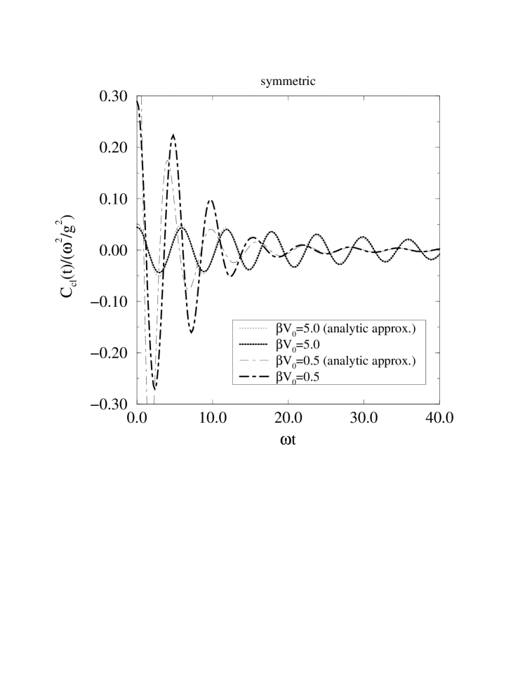
Figure 1: The classical correlator $C_{\rm cl}(t)$ in the symmetric case. The thin line represents the analytic approximation of Sec. 5.2. The difference between the thin and thick lines in the regime $1\mathop{\raise 1.29167pt\hbox{$<$\kern-7.5pt\raise-4.73611pt\hbox{$\sim$}}}\omega t\mathop{\raise 1.29167pt\hbox{$<$\kern-7.5pt\raise-4.73611pt\hbox{$\sim$}}}\beta V_{0}$ is due to higher order perturbative corrections in $1/\beta V_{0}\sim g^{2}/\beta\omega^{4}$.

Figure 2: The quantum correction $C_{\hbar^{2}}^{(a)}(t)+C_{\hbar^{2}}^{(b)}(t)$ in the symmetric case. We have divided out the naive expansion parameter $(\epsilon\beta V_{0})^{2}=({\frac{1}{4}}\beta\hbar\omega)^{2}$.

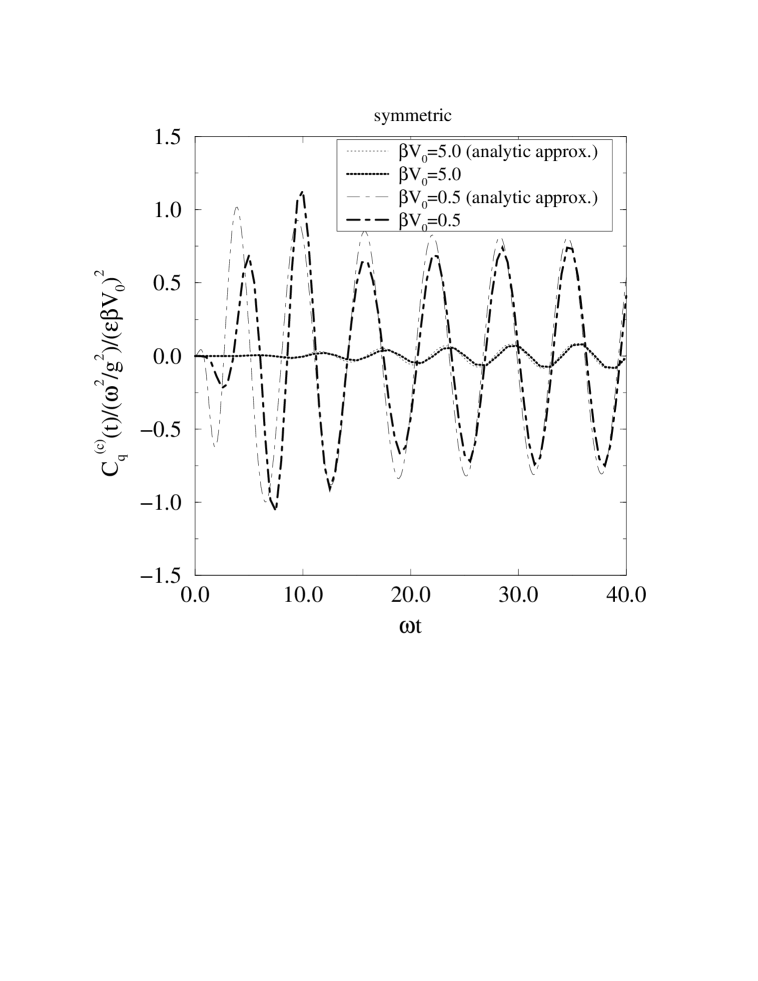
Figure 3: The quantum correction $C_{\hbar^{2}}^{(c)}(t)$ in the symmetric case, compared with the analytic approximation of Sec. 5.2.

The qualitative features of the solution are the following: Both the classical solution $C_{\rm cl}(t)$ and the quantum correction $C_{\hbar^{2}}^{(a)}(t)+C_{\hbar^{2}}^{(b)}(t)$ approach zero at large times. The time scale it takes for the amplitude to diminish depends on $\hat{\beta}$, being roughly proportional to $\hat{\beta}$, and being somewhat larger for the quantum corrections. The reason for the attenuation is the destructive interference of the continuum of classical solutions with different frequencies. This feature does not fully persist in the quantum case where the energy levels are discrete: rather the behaviour is “almost periodic” [21] on a larger time scale. Indeed, already the term $C_{\hbar^{2}}^{(c)}(t)$ in Fig. 3 behaves in a manner qualitatively different from $C_{\hbar^{2}}^{(a)}(t)$, $C_{\hbar^{2}}^{(b)}(t)$: it has a constant amplitude at large times.

Let us discuss these features and their implications in more quantitative terms.

5.2 The large time limit

We are mainly interested in the large time behaviour of the correlation function. Ordinary perturbation theory breaks down for large times and is therefore excluded. This is due to the secular terms in the perturbative series: at lowest order the solution to the classical equations of motion is proportional to $\cos(\omega t+\alpha)$ while the next order contains a term proportional to $g^{2}t\sin(\omega t+\alpha)$. Thus, by dimensional analysis, straightforward perturbation theory only works for

$$\hat{t}=\omega t\ll\frac{\omega^{4}}{g^{2}}\beta=4\beta V_{0}.$$ (5.1)

The way to avoid the secular terms is to use the exact frequency $\Omega(E)$ inside the trigonometric functions appearing in the perturbative series. The perturbative series for the classical solution of eq. (A.3) is obtained from eq. (C.6). In the phase space integration one then has to compute (after a change of variables according to eq. (A.15)) the dimensionless integrals

$$J_{nm}(\beta,t) = (\mbox{$\frac{g^{2}}{\omega^{4}}$})^{n+1}\int_{0}^{\infty}dEe^{-\beta E}E^{n}\cos(m\Omega(E)t),$$

$$\overline{J}_{nm}(\beta,t) = (\mbox{$\frac{g^{2}}{\omega^{4}}$)}^{n+1}\int_{0}^{\infty}dEe^{-\beta E}E^{n}\sin(m\Omega(E)t).$$ (5.2)

In general, this is difficult to do. Fortunately, an exact evaluation is not necessary if one is interested in the large time limit $\omega t\gg 1$. Then it is sufficient to keep only the first two terms of the low energy expansion of the exact frequency,

$$\Omega(E)=\omega\Bigl{[}1+{\frac{1}{4}}c_{1}\hat{E}+{\cal O}(\hat{E}^{2})\Bigr{]},$$ (5.3)

where $\hat{E}=E/V_{0}$ and $c_{1}=3/4$. In this approximation we find

$$J_{n1}(\beta,t) \approx n!\frac{\cos(\omega t+(n+1)\varphi)}{\Big{(}(\frac{\omega^{4}}{g^{2}}\beta)^{2}+(c_{1}\omega t)^{2}\Big{)}^{(n+1)/2}},$$

$$\overline{J}_{n1}(\beta,t) \approx n!\frac{\sin(\omega t+(n+1)\varphi)}{\Big{(}(\frac{\omega^{4}}{g^{2}}\beta)^{2}+(c_{1}\omega t)^{2}\Big{)}^{(n+1)/2}},$$ (5.4)

where

$$\varphi=\arcsin\left(\frac{c_{1}\omega t}{\sqrt{(\frac{\omega^{4}}{g^{2}}\beta)^{2}+(c_{1}\omega t)^{2}}}\right).$$ (5.5)

From these expressions one can see that in the region $\omega t\gg\frac{\omega^{4}}{g^{2}}\beta$ the terms which have been neglected in eq. (5.4) are suppressed by at least one power of $1/(\omega t)$. The reason is that each power of $E$ in the phase space integrand of eq. (5.2) gives one power of $1/(\omega t)$. In the region $1\ll\omega t\ll\beta V_{0}$, the terms neglected are suppressed by $g^{2}\beta/\omega^{4}$, corresponding to higher order perturbative corrections. Note that the approximation (5.4) is valid also for $\omega t\gg\beta V_{0}$ where the perturbative expansion breaks down. Thus the large time expansion for $C(t)$ can be obtained from the low energy expansion of the phase space integrand.

Using this expansion, we find for $C_{\rm cl}(t)$ for $\omega t\gg 1$,

$$C_{\rm cl}(t)\approx\frac{1}{\hbar Z_{\rm cl}}\frac{\omega^{5}}{g^{4}}J_{11}(\beta,t).$$ (5.6)

If $\hat{\beta}=\frac{\omega^{4}}{4g^{2}}\beta\gg 1$, there is an overlap of the “perturbative region” of eq. (5.1) and the large time region: for moderately large times $1\ll\omega t\ll\frac{\omega^{4}}{g^{2}}\beta$ we recover the leading order perturbative result. If $\omega t\gg\frac{\omega^{4}}{g^{2}}\beta$, in contrast, eq. (5.6) simplifies to

$$C_{\rm cl}(t)\approx-\frac{16}{9}\frac{1}{\hbar Z_{\rm cl}}\frac{\omega^{5}}{g^{4}}\frac{\cos\omega t}{(\omega t)^{2}}.$$ (5.7)

That is, for large times, the classical correlation function oscillates with the ’tree level’ frequency $\omega$ and with an amplitude which decreases as $1/t^{2}$. Comparing eq. (5.7) with the corresponding result for the harmonic oscillator, eq. (3.5), we see that eq. (5.7) is non-perturbative since its functional form cannot be obtained by adding corrections multiplied by positive powers of $g^{2}$ to the harmonic oscillator result.

Let us now note that if a resummation according to eq. (2.20) would take place, then the $\hbar^{2}$ quantum result should be obtained by replacing $\omega^{2}\to\omega_{\rm eff}^{2}$ in eq. (5.7), that is

$$C_{\hbar^{2}}^{\rm resummed}(t)\approx\biggl{[}1+b_{1}\frac{g^{2}\hbar^{2}\beta}{\omega^{2}}\biggr{]}C_{\rm cl}(t)+{\frac{2}{9}}\frac{1}{\hbar Z_{\rm cl}}\frac{\hbar^{2}\beta\omega^{3}}{g^{2}}\frac{\sin\omega t}{\omega t},$$ (5.8)

where $b_{1}$ is some number. We show below that the true $C_{\hbar^{2}}(t)$ is not of the form in eq. (5.8).

We start with $C_{\hbar^{2}}^{(a)}(t)$. It was pointed out already in Sec. 2 that this term is related to the replacement $\omega^{2}\to\omega_{\rm eff}^{2}$ in the Hamiltonian appearing in the Boltzmann factor. To be more specific, the term $\omega^{2}$ in $U^{\prime\prime}(q)$ cancels in eq. (2.13) and in the limit $\omega t\gg 1$ we find

$$C_{\hbar^{2}}^{(a)}(t)\approx\frac{1}{8}(\hbar g\beta)^{2}\langle q^{2}\rangle_{\rm cl}C_{\rm cl}(t).$$ (5.9)

The contribution proportional to $\langle q^{3}q_{c}(t)\rangle_{\rm cl}$, on the other hand, has one additional power of $E$ in the phase space integrand compared with the classical case and is thus suppressed by a factor $1/(\omega t)$. From eq. (5.9) it is obvious that the quantum correction $C_{\hbar^{2}}^{(a)}(t)$ shows the qualitative behaviour indicated in the first term in eq. (5.8): it is small compared with the classical result if $\beta\hbar\omega\ll 1$ and this holds even for arbitrarily large times.

Next we consider the quantum corrections containing the derivatives $\partial^{2}_{q}$, $\partial^{2}_{p}$ which we have denoted by $C_{\hbar^{2}}^{(b)}(t)$. These derivatives acting on the trigonometric functions in $qq_{c}(t)$ give extra factors of $t$. When expanding the integrand in powers of energy one has to count $t$ as $E^{-1}$. For $\omega t\gg 1$ we find

$$C_{\hbar^{2}}^{(b)}(t)\approx\frac{1}{48}\frac{1}{\hbar Z_{\rm cl}}\frac{\hbar^{2}\beta\omega^{3}}{g^{2}}\left\{4J_{01}(\beta,t)-9\omega t\overline{J}_{11}(\beta,t)-\frac{9}{4}(\omega t)^{2}J_{21}(\beta,t)\right\}.$$ (5.10)

The individual terms in the curly brackets behave as $\sin(\omega t)/(\omega t)$ for large times, which is the expected behaviour in eq. (5.8). Such a result would at the same time indicate that without resummation, the semiclassical expansion breaks down for

$$\omega t\mathop{\raise 1.29167pt\hbox{$>$\kern-7.5pt\raise-4.73611pt\hbox{$\sim$}}}\frac{\omega^{3}}{\hbar g^{2}}\frac{1}{\beta\hbar\omega},$$ (5.11)

when the correction term in eq. (5.8) is as large as the leading term. However, we find that this does not occur: in the limit $\omega t\gg 1$ the individual terms in the curly brackets in eq. (5.10) cancel at leading order in $1/(\omega t)$. Therefore the amplitude of $C_{\hbar^{2}}^{(b)}(t)$ decreases as $1/(\omega t)^{2}$ for large times. Thus $C_{\hbar^{2}}^{(b)}(t)$ is small compared with the classical result at high temperatures. The corresponding suppression factor, however, is not in general given by $(\beta\hbar\omega)^{2}$. There are terms proportional to $1/(\omega t)^{2}$ having different dependences on the temperature: expanding eq. (5.10) gives terms $\propto\beta^{2}$ while the subleading terms in the low energy expansion are proportional to $\beta$. We have not calculated these terms analytically. The numerical result for the sum of $C_{\hbar^{2}}^{(a)}(t)$ and $C_{\hbar^{2}}^{(b)}(t)$ is shown in Fig. 2.

Finally we consider the correction $C_{\hbar^{2}}^{(c)}(t)$. The result for $\omega t\gg 1$ is

$$C_{\hbar^{2}}^{(c)}(t)\approx\frac{9}{64}\frac{1}{\hbar Z_{\rm cl}}\frac{\hbar^{2}}{\omega^{4}}(\omega t)^{2}\{J_{21}(\beta,t)-\frac{1}{4}\omega t\overline{J}_{11}(\beta,t)\},$$ (5.12)

which for $\omega t\gg\frac{\omega^{4}}{g^{2}}\beta$ becomes

$$C_{\hbar^{2}}^{(c)}(t)\approx-\frac{1}{12}\frac{1}{\hbar Z_{\rm cl}}\frac{\hbar^{2}}{\omega}\cos\omega t.$$ (5.13)

Thus at large times $C_{\hbar^{2}}^{(c)}(t)$ oscillates with the “tree level frequency” but with a time independent amplitude. This behaviour is qualitatively different from the classical case. Comparing eqs. (5.7), (5.13) we see that $C_{\hbar^{2}}^{(c)}(t)$ becomes as large as the classical correlator for $t\sim t_{*}$ where

$$\omega t_{*}=\frac{\omega^{3}}{\hbar g^{2}}=\frac{1}{\epsilon},$$ (5.14)

and for $t>t_{*}$ the semiclassical approximation breaks down.

The correction in eq. (5.13) is clearly not of the form allowed by eq. (5.8). Since there is a term of a functional form not allowed and the allowed $\sin\omega t/(\omega t)$-term does not emerge, we conclude that a resummation according to eq. (2.20) does not take place in the large time limit. Neither can one understand the result as a resummation with a correction factor different from that in eq. (2.20). Since a resummation cannot be made, the semiclassical expansion breaks down at the time given by eq. (5.14).

It can be checked from Fig. 3 that for $\omega t\mathop{\raise 1.29167pt\hbox{$>$\kern-7.5pt\raise-4.73611pt\hbox{$\sim$}}}10$ the analytic approximation for $C_{\hbar^{2}}^{(c)}(t)$ indeed gives quite an accurate estimate of the exact numerical result.

To conclude, let us point out that the qualitative features found, together with the “almost periodic” behaviour [21] at time scales $t\mathop{\raise 1.29167pt\hbox{$>$\kern-7.5pt\raise-4.73611pt\hbox{$\sim$}}}t_{*}$, can be reproduced with the following approximation. Writing the full quantum result in eq. (2.4) in the energy basis, one gets

$$C(t)=Z^{-1}\mathop{\rm Re}\sum_{m,n}e^{-\beta E_{m}}e^{\frac{i}{\hbar}t(E_{m}-E_{n})}|\langle m|Q|n\rangle|^{2}.$$ (5.15)

Approximating the energy levels to first order in $g^{2}$,

$$E_{n}=\hbar\omega\left(n+{\frac{1}{2}}\right)+{\frac{3}{8}}\frac{g^{2}\hbar^{2}}{\omega^{2}}\left(n^{2}+n+{\frac{1}{2}}\right),$$ (5.16)

and the eigenstates to zeroth order, one gets

$$C(t)\simeq Z^{-1}\frac{\hbar}{2\omega}\sum_{m=0}^{\infty}(m+1)\left(e^{-\beta E_{m+1}}+e^{-\beta E_{m}}\right)\cos\!\left(\frac{E_{m+1}-E_{m}}{\hbar}\right)t.$$ (5.17)

The behaviour of this solution for small $\epsilon=\hbar g^{2}/\omega^{3}$ follows the classical solution in Fig. 1 until the time scale is of order $t\sim 4t_{*}=4/\epsilon$, but then the periodicity sets in so that at the time scale $t\sim 8t_{*}$, the structure around $t=0$ in the classical solution is repeated. This is the reason for the breakdown of the classical approximation.

6 The broken case

6.1 Preliminaries

In the broken case, the classical Hamiltonian is

$$H=V_{0}\Bigl{[}2\hat{p}^{2}+(\hat{q}^{2}-1)^{2}\Bigr{]}.$$ (6.1)

There exists, of course, an enormous literature on this system. In the present finite temperature context, it has been previously studied by Dolan and Kiskis [21] and by Bochkarev [22].

Quite a lot is known about the qualitative behaviour of $C(t)$. In general, the solution can be written as in eq. (5.15). Since the solution is a sum of periodic contributions corresponding to the different energy levels that can be excited, $C(t)$ is “almost periodic” [21]. In particular, the lowest frequency appearing is determined by

$$\Delta E=E_{1}-E_{0}\propto\hbar\omega\exp\left(-\frac{2\sqrt{2}}{3}\frac{\omega^{3}}{g^{2}\hbar}\right),$$ (6.2)

implying that the symmetry is restored already at $T=0$ [25] in the sense that the correlator averaged over a long enough time period vanishes. In contrast, the classical result $C_{\rm cl}(t)$ has a non-zero limiting value for $t\to\infty$, in which the symmetry is only partially restored and all the oscillations die out [21]. The oscillations die out, like in the symmetric case, due to the destructive interference of the continuum of classical solutions with different frequencies.

The fact alone that the classical result does not show the expected qualitative behaviour of the full result, indicates that the classical result is not generically applicable. We study this problem in more concrete terms below by evaluating the $\hbar^{2}$-corrections.

Note that, in seeming contrast to what was just pointed out, the system in eq. (6.1) has also been used to illustrate that the classical approximation is applicable to some real time problems [2]. The reason for the difference is that the situation we consider is different from the one in [2]: we have a strict equilibrium situation at a finite temperature $\beta^{-1}$, which is also what is considered in [21, 22] and which occurs in the real time sphaleron rate simulations. The consideration in [2], in contrast, concerns a non-equilibrium symmetry-restoring rate obtained by taking an initial state where the system is prepared in one of the minima. In the strict equilibrium case, one cannot define such a rate. Still, the problem of the general applicability of the classical approximation to real-time problems remains.

6.2 Numerical Results

The form of the classical solution $q_{c}(t)$ for the broken case is discussed in Appendix B. The numerically evaluated classical correlator $C_{\rm cl}(t)$ is shown in Fig. 4, and the quantum correction $C_{\hbar^{2}}^{(a)}(t)+C_{\hbar^{2}}^{(b)}(t)$ in Fig. 5.

The most notable difference with respect to the symmetric case is that there is a constant part in the broken case results. The energy integrand for $C_{\rm cl}(t)$ is for illustration shown in Fig. 6 where the emergence of the constant part from $\hat{E}<1$ can be seen. It is evident from Fig. 4 that the partial symmetry restoration in the classical result is the stronger the higher the temperature is [21], and from Fig. 5 that there is a further symmetry restoring effect from the quantum corrections. It is seen in Fig. 5 that at high temperatures ($\beta V_{0}\sim 0.5-2.0$) the quantum corrections are roughly proportional to the naive expansion parameter $(\epsilon\beta V_{0})^{2}=({\frac{1}{4}}\beta\hbar\omega)^{2}$ which has been factored out.

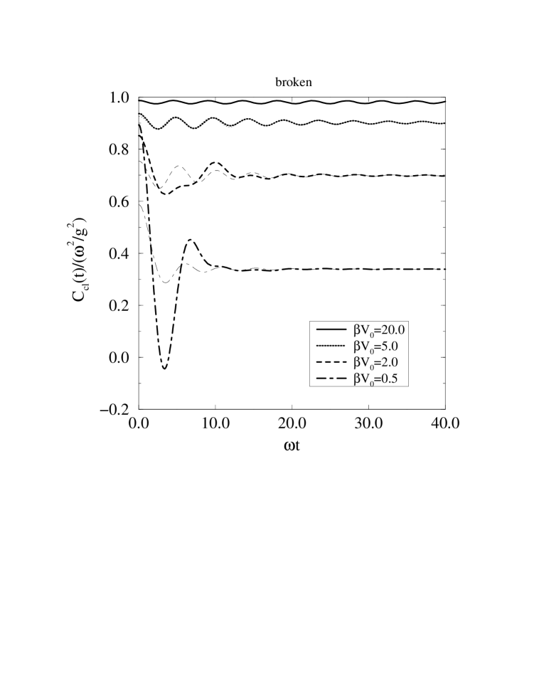
Figure 4: The classical correlator $C_{\rm cl}(t)$ in the broken case (thick lines), together with the analytic approximation of Sec. 6.3 (thin lines).

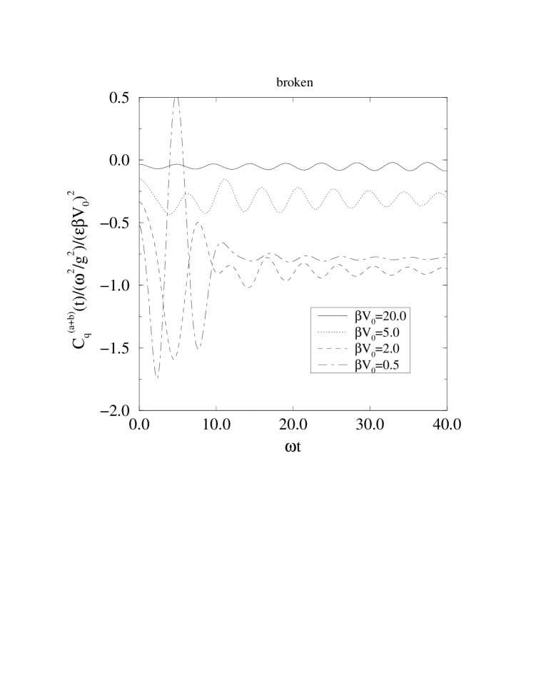
Figure 5: The quantum correction $C_{\hbar^{2}}^{(a)}(t)+C_{\hbar^{2}}^{(b)}(t)$ in the broken case.

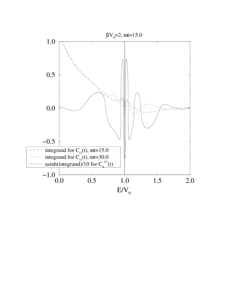
Figure 6: The energy integrands for $C_{\rm cl}(t)$ and $C_{\hbar^{2}}^{(c)}(t)$ in the broken symmetry case for $\beta V_{0}=2$. In the limit $\omega t\to\infty$ only the region $E/V_{0}<1$ contributes in $C_{\rm cl}(t)$. The energy integrand for $C_{\hbar^{2}}^{(c)}(t)$ has been shown on a logarithmic scale. It involves essentially the second derivative of the classical integrand, which is why it has very high peaks ($\sim 10^{10}$ already at $\omega t\sim 15$) around $E/V_{0}=1$.

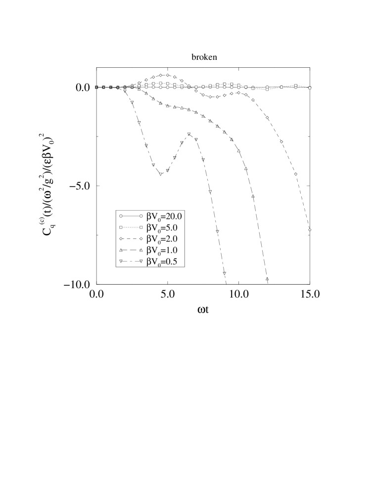
Figure 7: The quantum correction $C_{\hbar^{2}}^{(c)}(t)$ in the broken case, divided by $(\epsilon\beta V_{0})^{2}=({\frac{1}{4}}\beta\hbar\omega)^{2}$.

Let us then discuss $\hat{C}_{\hbar^{2}}^{(c)}(\hat{\beta},\hat{t})$. Its numerical evaluation turns out to be very difficult for large $\hat{t}$. The reason is that the energy-integrand is highly peaked and oscillatory around unity. To see this, note first that at $\hat{t}=0$, the integrand in eq. (A.12) vanishes. Moreover, the integrand involves terms $\sim\sin\hat{\Omega}(\hat{E})\hat{t}$, in analogy with eq. (6.8) below. Hence a particular energy region will contribute provided that

$$\hat{\Omega}(\hat{E})\hat{t}\mathop{\raise 1.29167pt\hbox{$>$\kern-7.5pt\raise-4.73611pt\hbox{$\sim$}}}1.$$ (6.3)

Let $y=|\hat{E}-1|\ll 1$. Since $K(k)\sim\ln(4/k^{\prime})$ close to $k=1$ ($k^{\prime}=\sqrt{1-k^{2}}$), one gets from eq. (B.4) that

$$\hat{\Omega}(\hat{E})=\left\{\begin{array}[]{ll}\frac{2\pi}{\ln(64/y)},&\hat{E}\mathop{\raise 1.29167pt\hbox{$<$\kern-7.5pt\raise-4.73611pt\hbox{$\sim$}}}1\\ \frac{\pi}{\ln(64/y)},&\hat{E}\mathop{\raise 1.29167pt\hbox{$>$\kern-7.5pt\raise-4.73611pt\hbox{$\sim$}}}1\end{array}\right..$$ (6.4)

Eq. (6.3) shows then that the energy-integrand can be large in the region

$$y\mathop{\raise 1.29167pt\hbox{$>$\kern-7.5pt\raise-4.73611pt\hbox{$\sim$}}}e^{-\hat{t}}.$$ (6.5)

On the other hand, the second partial derivative in eq. (A.12) will involve

$$\partial_{\hat{p}}^{2}\Omega(\hat{E})=(\partial_{\hat{p}}{\hat{E}})^{2}\partial_{\hat{E}}^{2}\Omega(\hat{E})+\ldots,$$ (6.6)

where $\partial_{\hat{p}}\hat{E}=4\hat{p}$. Hence according to eqs. (6.4), (6.5),

$$\frac{\partial^{2}\hat{q}_{c}(\hat{t}^{\prime})}{\partial\hat{p}^{2}}\sim\frac{1}{y^{2}}\mathop{\raise 1.29167pt\hbox{$<$\kern-7.5pt\raise-4.73611pt\hbox{$\sim$}}}e^{2\hat{t}}.$$ (6.7)

Thus the height of the peaks around $\hat{E}=1$ grows exponentially with time, and the peaks move closer to $\hat{E}=1$. The width of the peaks is diminishing, but their height is growing faster so that they give an increasing contribution. In fact, the highest peak’s contribution from $\hat{E}<1$ (where the peak gives a positive contribution) and from $\hat{E}>1$ (where it gives a negative one) to a large extent cancel, but the cancellation is not complete and one has to account for it very precisely in the numerics to get the remaining contribution correctly. This is why we cannot go to large $\hat{t}$. In practice, we can reliably calculate $\hat{C}_{\hbar^{2}}^{(c)}(\hat{\beta},\hat{t})$ only up to $\hat{t}=15$, when the highest peaks in the energy integrand are of height $\sim 10^{10}$ (for $\beta V_{0}\sim 2$) at $\delta\hat{E}\sim 10^{-5}$ around unity. The energy integrand is shown in Fig. 6 and the result of the integration in Fig. 7.

6.3 The large time limit

Consider first the classical correlation function. The form of the solutions in eq. (B.2) can be read off from eq. (C.6). It is seen that for $\hat{E}<1$, $q_{c}(t)$ contains a constant part in addition to the cosines. The $\phi$-integral obtained with the change of variables in eq. (A.15), gives then

$$\int_{-K(k)}^{K(k)}\!d\phi\,{\rm dn}_{k}(\phi){\rm dn}_{k}(w\hat{t}+\phi)=\frac{\pi^{2}}{2K(k)}\biggl{\{}1+8\sum_{n=1}^{\infty}\frac{q^{2n}}{(1+q^{2n})^{2}}\cos\!\left[{n\Omega(E)t}\right]\biggr{\}}.$$ (6.8)

The cosines in eq. (6.8) give contributions which vanish in the limit $t\to\infty$ as in eq. (5.4), see below. Hence one gets from eqs. (4.6), (A.15) that the constant part surviving is

$$C_{\rm cl}(t\to\infty)=\frac{\pi}{4}\frac{1}{\hbar Z_{\rm cl}}\frac{\omega^{5}}{g^{4}}\int_{0}^{1}d\hat{E}e^{-\hat{\beta}\hat{E}}\frac{w}{K(k)}.$$ (6.9)

One may also try to compute the time dependent part for $\omega t\gg 1$ in the same way as in the symmetric case. There we saw that the limiting behaviour for large times can be obtained from a suitable low energy expansion of the solution to the equations of motion. In the present case it is obvious that this expansion cannot be convergent when $\hat{E}$ approaches unity. One may argue, however, that for large times only the solutions with small energies are relevant and that this expansion still works. We find that

$$C_{\rm cl}(t)=C_{\rm cl}(t\to\infty)+\frac{1}{16\sqrt{2}}\frac{1}{\hbar Z_{\rm cl}}\frac{\omega^{5}}{g^{4}}\int_{0}^{1}d\hat{E}e^{-\hat{\beta}\hat{E}}\Bigg{(}\hat{E}\cos[\Omega(\hat{E})t]+{\cal O}(\hat{E}^{2})\Bigg{)}.$$ (6.10)

Replacing the upper integration limit by $\infty$ and keeping only the first two terms of the low energy expansion of

$$\Omega(\hat{E})=\sqrt{2}\omega(1-d_{1}\hat{E}+{\cal O}(\hat{E}^{2}))$$ (6.11)

where $d_{1}=3/16$, we obtain for $\omega t\gg 1$,

$$C_{\rm cl}(t)\approx C_{\rm cl}(t\to\infty)+\frac{1}{16\sqrt{2}}\frac{1}{\hbar Z_{\rm cl}}\frac{\omega^{5}}{g^{4}}\,\frac{\cos(\sqrt{2}\omega t-2\varphi)}{(\beta V_{0})^{2}+(d_{1}\sqrt{2}\omega t)^{2}},$$ (6.12)

where now

$$\varphi=\arcsin\left(\frac{d_{1}\sqrt{2}\omega t}{\sqrt{(\beta V_{0})^{2}+(d_{1}\sqrt{2}\omega t)^{2}}}\right).$$ (6.13)

It can be seen in Fig. 4 that eq. (6.12) is indeed a good approximation at large times.

The integrals appearing in the quantum corrections $C_{\hbar^{2}}^{(a)}(t)$ and $C_{\hbar^{2}}^{(b)}(t)$ are qualitatively quite similar to that appearing in $C_{\rm cl}(t)$. In particular, there is a constant part in these corrections which can be evaluated in the same way as eq. (6.9). It is seen that the constant part tends to further restore the symmetry compared with the classical result, see Fig. 5.

For the quantum correction $C_{\hbar^{2}}^{(c)}(t)$, in contrast, the “small energy expansion” does not seem to be applicable. We have computed the solution but it does not agree with Fig. 7. However, this need not be a surprise since, as discussed, it is not guaranteed that the small energy expansion works in the broken case due to the singular nature of the point $\hat{E}=1$: the energy integration extends beyond the radius of convergence of the small energy expansion. Moreover, the integrand in $C_{\hbar^{2}}^{(c)}(t)$ is qualitatively different from that in $C_{\rm cl}(t)$. A simple example where the small energy expansion would not work is given by

$$f(\hat{t})=\int_{0}^{\infty}d\hat{E}e^{-\hat{\beta}\hat{E}}\frac{\sin\hat{t}(1-\hat{E})}{\pi(1-\hat{E})}.$$ (6.14)

At $\hat{t}\to\infty$ the integrand makes a delta-function, and $f(\hat{t}\to\infty)\to\exp(-\hat{\beta})$. Yet an expansion in $\hat{E}$ of the denominator around $\hat{E}=0$ and an integration term by term, gives a result which oscillates around zero.

We could not find any other analytic way of evaluating the energy integral for $C_{\hbar^{2}}^{(c)}(t)$, either. The integrand is very complicated around $\hat{E}\sim 1$. Thus we can only mention some general features of the solution.

First, note that the numerical result in Fig. 7 shows that there is a growing negative contribution at large $\hat{t}$ in $C_{\hbar^{2}}^{(c)}(t)$. This seems to arise from $\hat{E}$ a bit larger than unity. To estimate very roughly when this kind of a contribution can be important, note that then the peak heights must be such that the exponential suppression cannot hide them any more, that is

$$e^{-\hat{\beta}}e^{2\hat{t}}\mathop{\raise 1.29167pt\hbox{$>$\kern-7.5pt\raise-4.73611pt\hbox{$\sim$}}}1.$$ (6.15)

Hence one starts to get an effect at $\hat{t}\mathop{\raise 1.29167pt\hbox{$>$\kern-7.5pt\raise-4.73611pt\hbox{$\sim$}}}\hat{\beta}$.

As to the functional form of the solution, it looks roughly like $-\hat{t}^{4}$ at large $\hat{t}$. It is easy to see that a linear in $\hat{t}$ behaviour cannot occur, since it follows directly from the definition in eq. (2.4) that $C(t)$ is symmetric in $t$. For $\beta V_{0}=0.5,1.0$ in which case the asymptotic behaviour is obtained earliest, the leading term of $C_{\hbar^{2}}^{(c)}(t)$ can be fitted at $\omega t\sim 8\ldots 15$ for instance as

$$C_{\hbar^{2}}^{(c)}(t)\sim\frac{\omega^{2}}{g^{2}}\epsilon^{2}\Bigl{[}-0.01(\omega t)^{4}\Bigr{]}.$$ (6.16)

The conclusions one can draw from the broken case seem rather similar to those from the symmetric case. The quantum correction $C_{\hbar^{2}}^{(c)}(t)$ behaves in a manner qualitatively different form what was observed for $C_{\rm cl}(t)$. Moreover, the difference is such that it cannot be accounted for by a simple resummation of the mass parameter $\omega^{2}$. As the classical result in Fig. 4 is of order unity and the fit in eq. (6.16) would suggest the behaviour $\epsilon^{2}(\omega t)^{4}$ for the quantum correction, one would expect that the semiclassical expansion breaks down at

$$\omega t\sim\omega t_{*}=\frac{1}{\sqrt{\epsilon}}=\biggl{(}\frac{\omega^{3}}{g^{2}\hbar}\biggr{)}^{1/2}.$$ (6.17)

In eq. (5.14) in the symmetric case it was rather observed that $\omega t_{*}=1/\epsilon$. However, the fit in eq. (6.16) should not be taken very seriously as the interval is very small, and the main point is that the time scale for the breakdown seems to be determined by $1/\epsilon$.

Finally, let us point out that from the general form of eq. (5.15), one might have expected that at finite temperature the asymptotic values of $C(t)$ are oscillating between positive and negative values. At zero temperature the time scale would be $\sim\exp[2\sqrt{2}/(3\epsilon)]$ according to eq. (6.2). Thus the quantum correction $C_{\hbar^{2}}^{(c)}(t)$ seems to restore some of the qualitative features missing in $C_{\rm cl}(t)$, in the sense that the behaviour in Fig. 7 looks like the beginning of an oscillation with a large time scale. The difference from the zero temperature case, however, is that the time scale associated with the oscillation is not exponential.

7 Summary and Conclusions

We have studied the classical finite temperature real time two-point correlation function and its first quantum corrections for the anharmonic oscillator. The expansion around the classical limit is made in powers of $\hbar$, so that each order contains all orders in the coupling constant $g^{2}$.

One can identify three different time scales in the results. In the symmetric case (Section 5), these are

$$\omega t\sim 1,\quad\omega t\sim\hat{\beta}\equiv\frac{\omega^{4}}{4g^{2}}\beta,\quad\omega t\sim\omega t_{*}=\frac{1}{\epsilon}\equiv\frac{\omega^{3}}{g^{2}\hbar}.$$ (7.1)

As long as $\omega t\ll\hat{\beta}$, perturbation theory works and the correlation function oscillates with period $\omega t\sim 1$. In the non-perturbative region $\omega t\mathop{\raise 1.29167pt\hbox{$>$\kern-7.5pt\raise-4.73611pt\hbox{$\sim$}}}\hat{\beta}$, the correlation function approaches its asymptotic form. We have developed a large time expansion which allows to address also the time scales $\omega t\gg\hat{\beta}$. In this regime the amplitude of the oscillations in the classical result attenuates due to the destructive interference of solutions to the equations of motion with different energies. This attenuation cannot be associated with a damping rate. Finally, the time scale $t_{*}$ is associated with the quantum corrections and becomes infinity in the formal limit $\hbar\to 0$. There is a hierarchy $\omega t_{*}\gg\hat{\beta}$ provided that $\beta\hbar\omega\ll 1$.

The general result of our study is that at the non-perturbative time scales $\omega t\mathop{\raise 1.29167pt\hbox{$>$\kern-7.5pt\raise-4.73611pt\hbox{$\sim$}}}\hat{\beta}$, the form of the quantum corrections differs qualitatively from that of the classical result. The semiclassical expansion breaks down at $t\sim t_{*}$ when the quantum corrections become as large as the classical result. Moreover, we found that these large corrections cannot be resummed by modifying the parameters of the classical theory.

On the other hand, the first quantum corrections to the classical correlation function are small for $t\ll t_{*}$. From this we would expect that in this region the classical limit gives a good approximation for the full quantum mechanical correlation function. The expansion parameter for the quantum corrections in this region is not just the naive one $(\beta\hbar\omega)^{2}$, but $\epsilon(\beta\hbar\omega)$ and $\epsilon^{2}$ appear, as well.

An essential question is then which of the discussed features might be carried over to field theory. Unfortunately, we cannot say very much about this. However, certainly the present study does not encourage one to believe in the generic applicability of the classical approximation in the high temperature limit for time-dependent quantities at arbitrarily large times. On the other hand, there are also obvious features which cannot hold in a four-dimensional field theory: for instance, we found that the time $t_{*}$ does not depend on the temperature. This is unlikely to be true in the pure SU(2) theory, say; dimensionally, the classical time scale not involving $\hbar$ is $(g^{2}T)^{-1}$ in that case and the time scale proportional to $\hbar^{-1}$ is $(\hbar g^{4}T)^{-1}$.

It would be interesting to extend the present type of an analysis to field theory to be able to make more concrete conclusions. Unfortunately, a straightforward evaluation of the quantum correction $C_{\hbar^{2}}^{(c)}(t)$ was numerically quite demanding even in the present case, in particular for the “broken” case where the modes with $E/V_{0}\sim 1$ are rather singular. In the field theory case, the partial derivatives of the classical solution with respect to the initial conditions would be replaced by functional derivatives, making things even more complicated. Still, one might hope that the scalar field theory analogue of the symmetric case would allow a non-perturbative investigation of the quantum corrections in the damping rate.

Finally, let us point out that as it appears that the classical approximation does not describe the large time behaviour at least in the present case, it would perhaps be useful to consider the feasibility of other approaches. In principle the problem can be solved non-perturbatively using Euclidean simulations and spectral function techniques. The anharmonic oscillator considered in this paper might be a suitable toy model for developing techniques for such studies, since it appears that there is some non-trivial structure even in this case.

Appendix Appendix A

In this appendix, we give some details concerning the classical solution $q_{c}(t)$ and the computation of the quantum corrections to $C_{\rm cl}(t)$ in the symmetric case. We use the rescaled variables defined in eq. (4.2).

The classical Hamiltonian is

$$H=V_{0}\Bigl{[}2\hat{p}^{2}+\hat{q}^{4}+2\hat{q}^{2}\Bigr{]}.$$ (A.1)

Let us introduce some useful notation:

$$k^{2} = \frac{2\sqrt{1+\hat{E}}}{\sqrt{1+\hat{E}}-1}\in(2,\infty),\quad k^{\prime 2}=1-k^{2}<0,\quad\tilde{k}=k^{-1}<1,$$

$$\hat{q}_{\rm max}^{2} = \sqrt{1+\hat{E}}-1,\quad w=\frac{\hat{q}_{\rm max}}{\sqrt{2}}.$$ (A.2)

The solution of the classical equations of motion is then of the form

$$\hat{q}_{c}(\hat{t})=\hat{q}_{\rm max}{\rm cn}_{\tilde{k}}(kw\hat{t}+k\phi),$$ (A.3)

where ${\rm cn}_{k}(u)$ is a Jacobi elliptic function (see Appendix C). Here the initial conditions of $\hat{q}_{c}(\hat{t})$ at $\hat{t}=0$ are given by

$$\hat{q}_{c}(0)=\hat{q}=\hat{q}_{\rm max}{\rm cn}_{\tilde{k}}(k\phi),\quad\dot{\hat{q}\,}_{c}(0)=\hat{p}=-\hat{q}_{\rm max}wk\,{\rm sn}_{\tilde{k}}(k\phi){\rm dn}_{\tilde{k}}(k\phi).$$ (A.4)

For $\hat{q}>0$ these can be inverted to give

$$\phi=-\mathop{\rm sign}(\hat{p})\tilde{k}F\biggl{(}\arcsin\!\sqrt{1-\frac{\hat{q}^{2}}{\hat{q}_{\rm max}^{2}}},\tilde{k}\biggr{)},$$ (A.5)

where $F(\phi,k)$ is the normal elliptic integral of the first kind (see Appendix C). If $\hat{q}<0$, one should replace the result in eq. (A.5) by

$$\phi\to 2\,{\rm sign}(\phi)\mathop{\rm Re}K(k)-\phi,$$ (A.6)

where

$$\mathop{\rm Re}K(k)\equiv\left\{\begin{array}[]{ll}K(k),&k<1\\ \tilde{k}K(\tilde{k}),&k>1\end{array}\right.$$ (A.7)

(the case $k<1$ is relevant in Appendix B). Note also that the frequency of the classical solution depends now, in contrast to the harmonic case, on the energy: according to Appendix C, the period of ${\rm cn}_{\tilde{k}}$ is $4K(\tilde{k})$ so that it follows from eq. (A.3) that

$$\hat{\Omega}(\hat{E})\equiv\frac{2\pi}{P(\hat{E})}=\frac{\pi w}{2\tilde{k}K(\tilde{k})},$$ (A.8)

where $P(\hat{E})$ is the period of $\hat{q}_{c}(\hat{t})$.

Given the classical solution, the classical correlation function $C_{\rm cl}(t)$ can be calculated from eq. (4.6). The classical partition function of eq. (4.7) is given by

$$\hat{Z}_{\rm cl}(\hat{\beta})=\sqrt{\frac{\pi}{2\hat{\beta}}}\int_{0}^{\infty}d\hat{q}e^{-\hat{\beta}(\hat{q}^{4}+2\hat{q}^{2})}=\frac{1}{4}\sqrt{\frac{\pi}{\hat{\beta}}}e^{\hat{\beta}/2}K_{{\frac{1}{4}}}(\hat{\beta}/2),$$ (A.9)

where $K_{\nu}(x)$ is the modified Bessel function of the second kind. The quantum corrections in eq. (4.8) are given by

$$\hat{C}_{\hbar^{2}}^{(a)}(\hat{\beta},\hat{t}) = 2\hat{\beta}^{2}\int_{-\infty}^{\infty}d\hat{p}\int_{0}^{\infty}d\hat{q}e^{-\hat{\beta}\hat{E}}\hat{q}^{2}[{\hat{Z}_{\rm cl}^{-1}}{\hat{C}_{\rm cl}(t)}-\hat{q}\hat{q}_{c}(\hat{t})],$$ (A.10)

$$\hat{C}_{\hbar^{2}}^{(b)}(\hat{\beta},\hat{t}) = \frac{4}{3}\hat{\beta}^{2}\int_{-\infty}^{\infty}d\hat{p}\int_{0}^{\infty}d\hat{q}e^{-\hat{\beta}\hat{E}}\Bigl{[}-(3\hat{q}^{2}+1)$$ (A.11)

$$\hskip 28.45274pt+2\hat{\beta}\hat{q}^{2}(\hat{q}^{2}+1)^{2}+2\hat{\beta}\hat{p}^{2}(3\hat{q}^{2}+1)\Bigr{]}\hat{q}\hat{q}_{c}(\hat{t}).$$

To get eq. (A.11) partial integrations with respect to $\hat{p}$ and $\hat{q}$ were performed.

Concerning $\hat{C}_{\hbar^{2}}^{(c)}(\hat{\beta},\hat{t})$, it is useful to make a canonical transformation to variables at time $\hat{t}^{\prime}$ to evaluate the Poisson bracket in eq. (2.15), to change then the time integration variable and to perform one partial integration with respect to $\hat{p}$. The result can be written as

$$\hat{C}_{\hbar^{2}}^{(c)}(\hat{\beta},\hat{t})=\frac{1}{4}\int_{-\infty}^{\infty}d\hat{p}\int_{0}^{\infty}d\hat{q}e^{-\hat{\beta}\hat{E}}\int_{0}^{\hat{t}}d{\hat{t}}^{\prime}\Bigl{[}4\hat{\beta}\hat{p}\hat{q}_{c}(\hat{t}^{\prime}-\hat{t})-\frac{\partial\hat{q}_{c}(\hat{t}^{\prime}-\hat{t})}{\partial\hat{p}}\Bigr{]}\hat{q}\frac{\partial^{2}\hat{q}_{c}(\hat{t}^{\prime})}{\partial\hat{p}^{2}}.$$ (A.12)

The partial derivatives of $\hat{q}_{c}(\hat{t}^{\prime})$ can be evaluated numerically, or even analytically using the formulas in [27]. As an example, the first derivative is

$$\frac{\partial\hat{q}_{c}(\hat{t})}{\partial\hat{p}} = \frac{\hat{p}}{2k^{2}}(2-k^{2})^{3}\hat{q}_{\rm max}\biggl{\{}-{\rm cn}_{\tilde{k}}v\biggl{[}\frac{\hat{q}_{\rm max}^{2}}{2}+\frac{{\tilde{k}}^{2}}{k^{\prime 2}}{\rm sn}_{\tilde{k}}^{2}v\biggr{]}$$ (A.13)

$$+{\rm sn}_{\tilde{k}}v{\rm dn}_{\tilde{k}}v\biggl{[}\frac{E_{\tilde{k}}(v)-E_{\tilde{k}}(k\phi)}{k^{\prime 2}}+\frac{wt}{k}\biggl{(}\hat{q}_{\rm max}^{2}+1\biggr{)}$$

$$-\frac{w}{kk^{\prime 2}}\frac{\hat{q}}{\hat{p}}\biggl{(}1-\frac{\hat{q}^{2}}{\hat{q}_{\rm max}^{2}}\biggr{)}-\frac{wk\hat{q}_{\rm max}^{2}}{2}\frac{\hat{q}}{\hat{p}}\biggr{]}\biggr{\}}_{v=kw\hat{t}+k\phi},$$

where $E_{\tilde{k}}(v)$ is defined in eq. (C.4).

Finally, note that since the variable $\phi$ appears in a simple manner in $\hat{q}_{c}(\hat{t})$ in eq. (A.3), it is convenient to make a change of integration variables. We go first into the canonical action-angle variables $(I,\alpha)$, and then from these into energy $E$ and the variable $\phi$, using

$$\frac{\partial I(E)}{\partial E}=\frac{1}{\Omega(E)},\quad\frac{\partial\alpha}{\partial\phi}=\frac{\Omega(E)}{w}.$$ (A.14)

The integration measure can then be written as

$$\int_{-\infty}^{\infty}d\hat{p}\int_{0}^{\infty}d\hat{q}\,[\ldots]=\int_{0}^{\infty}d\hat{E}\int_{-\mathop{\rm Re}K(k)}^{\mathop{\rm Re}K(k)}d\phi\frac{1}{4w}[\ldots].$$ (A.15)

Appendix Appendix B

In this appendix, we describe the classical solution $q_{c}(t)$ and formulas for the quantum corrections to $C_{\rm cl}(t)$ in the broken case. The classical Hamiltonian is in eq. (6.1).

In accordance with eq. (A.2), let us introduce some notation:

$$k^{2} = \frac{2\sqrt{\hat{E}}}{1+\sqrt{\hat{E}}}\in(0,2),\quad k^{\prime 2}=1-k^{2},\quad\tilde{k}=k^{-1},$$

$$\hat{q}_{\rm max}^{2} = 1+\sqrt{\hat{E}},\quad w=\frac{\hat{q}_{\rm max}}{\sqrt{2}}.$$ (B.1)

Then the classical solution is

$$\hat{q}_{c}(\hat{t})=\left\{\begin{array}[]{ll}\pm\hat{q}_{\rm max}{\rm dn}_{k}(w\hat{t}+\phi),&\hat{E}<1\\ \hat{q}_{\rm max}{\rm cn}_{\tilde{k}}(kw\hat{t}+k\phi),&\hat{E}>1\end{array}\right.,$$ (B.2)

where the relation to $\hat{p},\hat{q}$ is (for $\hat{q}>0$)

$$\phi=\left\{\begin{array}[]{ll}-\mathop{\rm sign}(\hat{p})F\biggl{(}\arcsin\!\sqrt{\frac{1}{k^{2}}\biggl{(}{1-\frac{\hat{q}^{2}}{\hat{q}_{\rm max}^{2}}}\biggr{)}},k\biggr{)},&\hat{E}<1\\ -\mathop{\rm sign}(\hat{p})\tilde{k}F\biggl{(}\arcsin\!\sqrt{1-\frac{\hat{q}^{2}}{\hat{q}_{\rm max}^{2}}},\tilde{k}\biggr{)},&\hat{E}>1\end{array}\right..$$ (B.3)

Note that $\hat{E}<1$ corresponds to modes which do not cross the barrier, whereas the $\hat{E}>1$ modes do cross it. The frequency of the classical solution again depends on energy and is given by

$$\hat{\Omega}(\hat{E})=\frac{2\pi}{P(\hat{E})}=\left\{\begin{array}[]{ll}\frac{\pi w}{K(k)},&\hat{E}<1\\ \frac{\pi w}{2\tilde{k}K(\tilde{k})},&\hat{E}>1\end{array}\right..$$ (B.4)

The classical partition function of eq. (4.7) is

$$\hat{Z}_{\rm cl}(\hat{\beta})=\sqrt{\frac{\pi}{2\hat{\beta}}}\int_{0}^{\infty}d\hat{q}e^{-\hat{\beta}(\hat{q}^{2}-1)^{2}}=\frac{1}{4}\sqrt{\frac{\pi}{\hat{\beta}}}e^{-\hat{\beta}/2}\Big{[}\sqrt{2}\pi I_{{\frac{1}{4}}}(\hat{\beta}/2)+K_{{\frac{1}{4}}}(\hat{\beta}/2)\Big{]},$$ (B.5)

where $I_{\nu},K_{\nu}$ are modified Bessel functions. The quantum corrections to the classical result of eq. (4.6) are

$$\hat{C}_{\hbar^{2}}^{(a)}(\hat{\beta},\hat{t}) = 2\hat{\beta}^{2}\int_{-\infty}^{\infty}d\hat{p}\int_{0}^{\infty}d\hat{q}e^{-\hat{\beta}\hat{E}}\hat{q}^{2}[{\hat{Z}_{\rm cl}}^{-1}{\hat{C}_{\rm cl}(t)}-\hat{q}\hat{q}_{c}(\hat{t})],$$ (B.6)

$$\hat{C}_{\hbar^{2}}^{(b)}(\hat{\beta},\hat{t}) = \frac{4}{3}\hat{\beta}^{2}\int_{-\infty}^{\infty}d\hat{p}\int_{0}^{\infty}d\hat{q}e^{-\hat{\beta}\hat{E}}\Bigl{[}(1-3\hat{q}^{2})$$ (B.7)

$$\hskip 28.45274pt+2\hat{\beta}\hat{q}^{2}(\hat{q}^{2}-1)^{2}+2\hat{\beta}\hat{p}^{2}(3\hat{q}^{2}-1)\Bigr{]}\hat{q}\hat{q}_{c}(\hat{t}).$$

The correction $\hat{C}_{\hbar^{2}}^{(c)}(\hat{\beta},\hat{t})$ is given by eq. (A.12). The partial derivatives of $\hat{q}_{c}(\hat{t}^{\prime})$ with respect to $\hat{p}$ can again be evaluated analytically. For example, for $\hat{E}<1$ we get

$$\frac{\partial\hat{q}_{c}(\hat{t})}{\partial\hat{p}} = \frac{\hat{p}}{2k^{2}}(2-k^{2})^{3}\hat{q}_{\rm max}\biggl{\{}{\rm dn}_{k}u\biggl{[}\frac{\hat{q}_{\rm max}^{2}}{2}-\frac{{\rm sn}_{k}^{2}u}{k^{\prime 2}}\biggr{]}$$ (B.8)

$$+{\rm sn}_{k}u{\rm cn}_{k}u\biggl{[}\frac{E_{k}(u)-E_{k}(\phi)}{k^{\prime 2}}-wt\biggl{(}\frac{\hat{q}_{\rm max}^{2}k^{2}}{2}+1\biggr{)}$$

$$-\frac{1}{k^{\prime 2}w}\frac{\hat{p}}{\hat{q}}+\hat{q}_{\rm max}^{2}w\frac{\hat{q}^{2}-1}{\hat{q}\hat{p}}\biggr{]}\biggr{\}}_{u=w\hat{t}+\phi},$$

and for $\hat{E}>1$ the expression is the one in eq. (A.13) with the replacement $\hat{q}_{\rm max}^{2}\to-\hat{q}_{\rm max}^{2}$, except for the $\hat{q}_{\rm max}^{2}$ appearing in $\hat{q}^{2}/\hat{q}_{\rm max}^{2}$.

Finally, a change of integration variables can be made according to eq. (A.15).

Appendix Appendix C

We discuss here briefly some of the basic definitions of the Jacobi elliptic functions used. The notation follows [26, 27].

Let $F(\phi,k)$ be the normal elliptic integral of the first kind,

$$F(\phi,k)=\int_{0}^{\phi}\frac{d\alpha}{\sqrt{1-k^{2}\sin^{2}\!\alpha}}.$$ (C.1)

Then the complete elliptic integral of the first kind $K(k)$ is defined by

$$K(k)=F(\frac{\pi}{2},k)=\int_{0}^{1}\frac{dt}{\sqrt{(1-t^{2})(1-k^{2}t^{2})}}.$$ (C.2)

The associated nome is

$$q=\exp\biggl{[}-\pi\frac{K(k^{\prime})}{K(k)}\biggr{]},$$ (C.3)

where $k^{\prime 2}=1-k^{2}$. Similarly,

$$E(\phi,k) = \int_{0}^{\phi}\!d\alpha\sqrt{1-k^{2}\sin^{2}\alpha},\quad u=\int_{0}^{\mathop{\rm am}_{k}u}\frac{d\alpha}{\sqrt{1-k^{2}\sin^{2}\alpha}},$$

$$E_{k}(u) \equiv E({\rm am}_{k}u,k)$$ (C.4)

define the normal elliptic integral of the second kind $E(\phi,k)$, the amplitude function ${\rm am}_{k}u$, and the function $E_{k}(u)$.

The Jacobi elliptic functions are denoted by ${\rm dn}_{k}u,{\rm sn}_{k}u,{\rm cn}_{k}u$. They are defined by ($0<u<K(k)$)

$$u = \int_{{\rm dn}_{k}u}^{1}\frac{dt}{\sqrt{(1-t^{2})(t^{2}-k^{\prime 2})}}=\int_{{\rm cn}_{k}u}^{1}\frac{dt}{\sqrt{(1-t^{2})(k^{\prime 2}+k^{2}t^{2})}}$$ (C.5)

$$= \int_{0}^{{\rm sn}_{k}u}\frac{dt}{\sqrt{(1-t^{2})(1-k^{2}t^{2})}}.$$

Note that ${\rm sn}_{k}u=\sin({\rm am}_{k}u)$. The periodicity of ${\rm dn}_{k}u$ is $2K(k)$, and that of ${\rm sn}_{k}u,{\rm cn}_{k}u$ is $4K(k)$; ${\rm dn}_{k}u,{\rm cn}_{k}u$ are symmetric while ${\rm sn}_{k}u$ is anti-symmetric. The functions appearing in the classical solution $q_{c}(t)$ for the anharmonic oscillator are ${\rm dn}_{k}u$ and ${\rm cn}_{k}u$. We need their Fourier expansions,

$${\rm dn}_{k}u = \frac{\pi}{2K(k)}\biggl{[}1+4\sum_{n=1}^{\infty}\frac{q^{n}}{1+q^{2n}}\cos\frac{n\pi u}{K(k)}\biggr{]},$$

$${\rm cn}_{k}u = \frac{2\pi}{kK(k)}\sum_{n=1}^{\infty}\frac{q^{n-1/2}}{1+q^{2n-1}}\cos\!\frac{(n-{1\over 2})\pi u}{K(k)},$$ (C.6)

where $q$ is the nome in eq. (C.3).

References

- [1] V.A. Kuzmin, V.A. Rubakov and M.E. Shaposhnikov, Phys. Lett. B 155 (1985) 36.
- [2] V.A. Rubakov and M.E. Shaposhnikov, Usp. Fis. Nauk 166 (1996) 493 [hep-ph/9603208].
- [3] P. Arnold and L. McLerran, Phys. Rev. D 36 (1987) 581.
- [4] S.Yu. Khlebnikov and M.E. Shaposhnikov, Nucl. Phys. B 308 (1988) 885.
- [5] O. Philipsen, Phys. Lett. B 358 (1995) 210.
- [6] D.Yu. Grigoriev and V.A. Rubakov, Nucl. Phys. B 299 (1988) 67.
- [7] J. Ambjørn, T. Askgaard, H. Porter and M.E. Shaposhnikov, Phys. Lett. B 244 (1990) 479; Nucl. Phys. B 353 (1991) 346; J. Ambjørn and K. Farakos, Phys. Lett. B 294 (1992) 248.
- [8] J. Ambjørn and A. Krasnitz, Phys. Lett. B 362 (1995) 97.
- [9] G.D. Moore, Nucl. Phys. B 480 (1996) 657; Nucl. Phys. B 480 (1996) 689; G.D. Moore and N. Turok, PUPT-1681 [hep-ph/9703266].
- [10] G.D. Moore and N. Turok, Phys. Rev. D 55 (1997) 6538.
- [11] W-H. Tang and J. Smit, Nucl. Phys. B 482 (1996) 265.
- [12] G. Aarts and J. Smit, Phys. Lett. B 393 (1997) 395.
- [13] W-H. Tang and J. Smit, ITFA-97-02 [hep-lat/9702017].
- [14] H.B. Nielsen, H.H. Rugh and S.E. Rugh, hep-th/9611128.
- [15] D. Bödeker, L. McLerran and A. Smilga, Phys. Rev. D 52 (1995) 4675.
- [16] P. Arnold, D. Son and L.G. Yaffe, Phys. Rev. D 55 (1997) 6264.
- [17] P. Huet and D.T. Son, Phys. Lett. B 393 (1997) 94.
- [18] C.R. Hu and B. Müller, DUKE-TH-96-133 [hep-ph/9611292].
- [19] P. Arnold, UW-PT-97-2 [hep-ph/9701393].
- [20] D. Bödeker, Nucl. Phys. B 486 (1997) 500 [hep-th/9609170].
- [21] L. Dolan and J. Kiskis, Phys. Rev. D 20 (1979) 505.
- [22] A. Bochkarev, Phys. Rev. D 48 (1993) 2382.
- [23] P. Ginsparg, Nucl. Phys. B 170 (1980) 388; T. Appelquist and R. Pisarski, Phys. Rev. D 23 (1981) 2305; S. Nadkarni, Phys. Rev. D 27 (1983) 917.
- [24] K. Kajantie, M. Laine, K. Rummukainen and M. Shaposhnikov, Nucl. Phys. B 458 (1996) 90 [hep-ph/9508379]; E. Braaten and A. Nieto, Phys. Rev. D 53 (1996) 3421; A. Jakovác and A. Patkós, hep-ph/9609364.
- [25] A.M. Polyakov, Nucl. Phys. B 120 (1977) 429.
- [26] E.T. Whittaker and G.N. Watson, Modern Analysis, 4th ed., Ch. 22 (Cambridge University Press, 1950).
- [27] P.F. Byrd and M.D. Friedman, Handbook of elliptic integrals for engineers and physicists (Springer-Verlag, 1954).