May 1997 CERN-TH/97-98

hep-ph/9705307

Dynamical Soft Terms with Unbroken Supersymmetry

S. Dimopoulos^(a,b), G. Dvali^(a), R. Rattazzi^(a), and G.F. Giudice^(a)

^(a)Theory Division, CERN
CH-1211 Geneva 23, Switzerland

^(b) Physics Department, Stanford University
Stanford, CA 94305, USA

We construct a class of simple and calculable theories for the supersymmetry breaking soft terms. They are based on quantum modified moduli spaces. These theories do not break supersymmetry in their ground state; instead we postulate that we live in a supersymmetry breaking plateau of false vacua. We demonstrate that tunneling from the plateau to the supersymmetric ground state is highly supressed. At one loop, the plateau develops a local minimum which can be anywhere between $10^{8}$ GeV and the grand unification scale. The value of this minimum is the mass of the messengers of supersymmetry breaking. Primordial element abundances indicate that the messengers’ mass is smaller than $10^{12}$ GeV.

1 Introduction

Gauge mediated theories of supersymmetry breaking [1] have recently attracted a great deal of attention becuse they solve the supersymmetric flavor problem. Beginning with the pioneering papers of Dine, Nelson and collaborators [2], a lot of effort has been devoted to the construction of explicit realistic models with dynamical supersymmetry breaking [3]-[8]. It seems fair to say that these models, when they work, are quite involved.

In this paper we wish to show how to construct simple theories of the supersymmetry breaking soft terms. The key ingredient that will allow us to do that is to relax the requirement that supersymmetry is spontaneously broken in the full theory. We instead will be content to postulate that we live in a supersymmetry breaking local minimum located on a plateau of flat directions.

In section 2 we will present the general class of theories we consider. In section 3 we will demonstrate the it is not dangerous to live on a plateau: the tunneling amplitude into the supersymmetry preserving true vacuum is infinitesimally small. In section 4 we will present explicit models implementing the ideas of section 2. In section 5 we will show that light element abundances place a limit that the messenger mass –which is related to the position of the local minimum in field space– has to be less than $10^{12}$ GeV. We conclude in section 6 with some brief comparisons of our models with earlier work.

2 The General Idea

We are interested in theories based on a gauge group

$$G=SU(5)_{W}\times G_{B}\times G_{S}.$$ (1)

By $SU(5)_{W}$ we mean indeed $SU(3)\times SU(2)\times U(1)$ as the dynamics we describe takes place below the GUT scale. Nonetheless, as we want to preserve perturbative gauge unification, we will only consider messenger sectors involving complete $SU(5)_{W}$ multiplets. The role of the remaining factors, as it will be clear below, is to provide a stable vacuum with broken supersymmetry. We consider the following simple form for the messenger sector superpotential

$$W=\lambda_{1}Rq\bar{q}+\lambda_{2}RQ\bar{Q}$$ (2)

where $R$ transforms non trivially only under $G_{B}$. The $q\oplus\bar{q}$ are vectorial under $SU(5)_{W}$, i.e. ${\bf 5}\oplus{\bf\bar{5}}$, but singlets of $G_{S}$. Finally, $Q\oplus\bar{Q}$ are a vectorial representation of $G_{S}$, but singlets of $SU(5)_{W}$. All the fields transform non-trivially under $G_{B}$. Just to make contact with usual gauge mediated models, we anticipate that the $q,\bar{q}$ will be play the role of the messengers, the $Q,\bar{Q}$ will provide a scale via their condensation, and $R$ will play the role of the usual $X$ field getting both a scalar and an $F$ component vacuum expectation value (VEV) from the strong dynamics.

Furthermore we are interested in theories with the following two properties at the classical level:

I)

$R$ contains just one $D$-flat direction, or equivalently there exist just one holomorphic invariant $u=u(R)\sim R^{k}$, which is a monomial made out of $R$ elements and $k$ is an integer. Along this flat direction the gauge factor $G_{B}$ is broken to a subgroup $H_{B}$ and all elements in $R$ but one, which we parametrize by $u$, are eaten by the SuperHiggs mechanism. For notational purposes we will in what follows parametrize the flat direction with a field $X=u^{1/k}\sim R$, since this is the one with canonical Kähler metric at large field values.

II)

Along $u$ the $q,\bar{q}$ and $Q,\bar{Q}$ pair up to get masses which are respectively $\sim\lambda_{1}R$ and $\sim\lambda_{2}R$.

Thus far away along $u\not=0$ the low energy theory has gauge group $G=SU(5)_{W}\times H_{B}\times G_{S}$ and the sole matter content is given by the MSSM fields plus the gauge singlet $u$. The additional group factors are just pure gauge with no matter. Furthermore we are going to assume that the only sizeable non perturbative low energy dynamics is the one associated with $G_{S}$. On a case by case basis we will check that $H_{B}$ is either too weak or it does not affect the effective superpotential. Above the scale of $G_{S}$ confinement the effective theory has $W=0$. The effective holomorphic scale $\Lambda_{eff}$ of the low energy $G_{S}$ theory is given by the 1-loop matching of the gauge couplings in the microscopic and macroscopic theories at the scale $X$ [9]

$$\Lambda_{eff}^{3\mu_{G_{S}}}=\Lambda^{3\mu_{G_{S}}-\mu_{Q}}(\lambda_{2}X)^{\mu_{Q}}$$ (3)

where $\mu_{G_{S}}$ and $\mu_{Q}$ are the Dynkin indices for the adjoint and $Q\oplus\bar{Q}$ representations of $G_{S}$. Below the scale $\Lambda_{eff}$ the $G_{S}$ charges are confined in massive states, and the only effect of the $G_{S}$ dynamics on the low energy theory is to generate a superpotential for $X$ via gaugino condensation [10, 11]

$$W_{eff}=<\lambda_{S}\lambda_{S}>=\Lambda_{eff}^{3}=\Lambda^{3-\mu_{Q}/\mu_{G_{S}}}(\lambda_{2}X)^{\mu_{Q}/\mu_{G_{S}}}.$$ (4)

In the limit in which the other gauge group factors are treated as weak the above result is exact. It can indeed be established by using holomorphy and an $R$-symmetry which has no $G_{S}$ anomaly [12]. Under this symmetry $X$ has charge $2\mu_{G_{S}}/\mu_{Q}$, consistent with the above $W_{eff}$ having charge 2.

The further requirement that we are going to make in order to generally characterize our models is that $\mu_{Q}=\mu_{G_{S}}$. For the class of theories that satisfy this identity $W_{eff}$ is linear in $X$

$$W_{eff}=\lambda_{2}\Lambda^{2}X.$$ (5)

An example of this possibility is given by $G_{S}=SU(N)$ with $Q+\bar{Q}$ corresponding to $N$ flavors of fundamentals. This is the crucial property that allows us to build simple and realistic theories with locally broken supersymmetry. Eq. (5) corresponds in fact to the simplest O’Raifertaigh model: $F_{X}=\partial_{X}W_{eff}=\lambda_{2}\Lambda^{2}$, so that supersymmetry is broken at any point on the $X$ complex line. For $\mu_{Q}\not=\mu_{G_{S}}$ the scalar potential $|\partial_{X}W_{eff}|^{2}$ would push $X$ either to the origin or to infinity, where supersymmetry is in general restored. Indeed, in models with the simple microscopic superpotential in eq. 2, at the point $X=0$ there are in general other flat directions involving the massless $q$ and $Q$, where supersymmetry can be restored. The existence of a plateau $V_{eff}\sim|\partial_{X}W_{eff}|^{2}\sim\lambda_{2}^{2}\Lambda^{4}$ insures that $X$ may stabilize in some other way far away from supersymmetry restoring points. This is the novelty of the models we discuss: there is no need to break supersymmetry in the true ground state.

The result in eq. (5) can also be derived by using the superpotential from confinement derived in Ref. [13] (see also Ref. [14]) and by integrating out the massive composite superfields.

Up to this point we have devised a general class of models for which there exists a direction $X$ in field space along which $W_{eff}\propto X$. In such a situation the curvature of the scalar potential is completely determined by the Kähler metric. We are interested in the region $\lambda_{2}X\gg\Lambda$, where it is consistent to consider only the perturbative corrections to the Kähler potential. These we know how to calculate. The tree level Kähler potential is given by (see eg. Ref. [15]) $K_{tree}=(uu^{\dagger})^{1/k}=XX^{\dagger}$. The radiative corrections are due to loops involving the heavy superfields $Q,\bar{Q}$ and $q,\bar{q}$ and the heavy vector superfields in the coset $G_{B}/H_{B}$. All these particles get a mass from the $X$ VEV. At the 1-loop level the result has the form

$$K(X,X^{\dagger})=XX^{\dagger}\left[1+{1\over 16\pi^{2}}\bigl{(}C_{B}g_{B}^{2}-C_{1}\lambda_{1}^{2}-C_{2}\lambda_{2}^{2}\bigr{)}\ln(XX^{\dagger}/M_{Pl}^{2})+\dots\right]$$ (6)

where the $C$’s are positive Casimirs and the coefficient of the logarithm just corresponds to the 1-loop anomalous dimension of the original field $R$. For large logarithms the higher loop terms can be resummed via the Renormalization Group (RG) so that in the leading log approximation the Kähler metric reads

$$K(X,X^{\dagger})=XX^{\dagger}Z_{R}\left(XX^{\dagger}/M_{Pl}^{2}\right).$$ (7)

In the above, $Z_{R}$ represents the $R$ wave function renormalization and $X$ the bare field. Then the effective potential is just given by

$$V_{eff}={|\partial_{X}W|^{2}\over\partial_{X}\partial_{X^{\dagger}}K}\simeq{\lambda_{2}^{2}\Lambda^{4}\over Z_{R}(XX^{\dagger})}$$ (8)

where we have approximated $\partial_{X}\partial_{X^{\dagger}}K$ with $Z(XX^{\dagger})$, neglecting small finite corrections. The logarithmic evolution of $Z_{R}$ with $|X|$ can generate local minima in the effective potential. Indeed the potential energy behaves qualitatively like a squared effective Yukawa coupling. As it can be inferred already from eq. (6), in the limit in which $g_{B}\ll\lambda_{1},\lambda_{2}$ we have that $1/Z_{R}$ grows at large $X$ thereby preventing a runaway behaviour. Indeed one can see this as a signal of the fact that pure Yukawa theories become strong in the ultraviolet by developing a Landau pole. On the other hand, in the opposite limit of $g_{B}\gg\lambda_{1},\lambda_{2}$ the potential grows at small $X$. This can prevent $X$ from reaching the origin or other branches of moduli space where supersymmetry may be restored. It is thus clear that the competition between these two effects, which arises when $\lambda_{1,2}\sim g_{B}$ may stabilize the potential at some local minimum $X_{0}$. Notice that it is crucial that $X$ comes form a field $R$ which is charged under some gauge group $G_{B}$. This is precisely what provides the gauge contribution $g_{B}^{2}$ without which $X$ is always pushed towards the origin, where we loose control of our approximation (and in most cases restore supersymmetry). The location of this $X_{0}$ is determined by the stationary point of the RG equation for $Z_{R}$

$$8\pi^{2}{d\ln Z_{R}\over d\ln|X|}=C_{B}g_{B}^{2}(|X|)-C_{1}{\lambda_{1}^{2}\over Z_{R}Z_{q}Z_{\bar{q}}}-C_{2}{\lambda_{2}^{2}\over Z_{R}Z_{Q}Z_{\bar{Q}}}=0$$ (9)

where $g_{B}$ and the $Z$’s are respectively the running gauge coupling and wave functions (of the various fields) evaluated at the scale $X$, while $\lambda_{1,2}$ are the bare Yukawa couplings, i.e. renormalized at the cut-off scale $M_{Pl}$. Then the expressions multiplying $C_{1}$ and $C_{2}$ represent respectively the effective running Yukawa couplings $\bar{\lambda}_{1}^{2}(X)$ and $\bar{\lambda}_{2}^{2}(X)$. This is just the usual Coleman-Weinberg mechanism. We have a “perturbative” dimensional transmutation, by which it is consistent to expect the minimum $X_{0}$ to be in the range $\Lambda\ll X_{0}\ll M_{\rm Pl}$. As we will explain in detail in the next sections, this is precisely the range which is interesting for building realistic models. It is also the range for which the minimum on the plateau, even if it is not the true ground state, is nonetheless stable on cosmological time scales (see the next section). Finally, to be more precise, in order to insure that the stationary point be a minimum one should verify that $d^{2}Z_{R}/d(\ln X)^{2}$ be negative. This equation, see eq. (9), involves both the gauge $\beta$-function and the $\gamma$’s of the other fields, and has to be checked case by case.

Before going further we would like to remark that this mechanism for stabilizing a tree level flat potential in a supersymmetric theory is just Witten’s inverse hierarchy [16]. The amusing and new thing is that in our case the superpotential is generated non-perturbatively rather than being an input at tree level. In other words we have a double dimensional transmutation

1)

$<F_{X}>=\lambda_{2}\Lambda^{2}$ is provided by gaugino condensation.

2

) $<X>$ is stabilized at some point by the Coleman-Weinberg mechanism.

It is interesting that in the region $X\gg\Lambda$ we can determine the exact superpotential together with a fairly accurate perturbative approximation to the Kähler potential. This allows us to safely control the full scalar lagrangian. We stress once more that, as in Witten’s model, it is crucial that $X$ be part of a charged multiplet in order to have balancing gauge and Yukawa contributions in $V_{eff}$. The issue of how a non-perturbative superpotential is stabilized by RG evolution is a subtle one, and our result disagrees with ref. [17]. The conclusion of that paper is that $V_{eff}\sim\lambda^{2}\Lambda^{4}/Z_{R}Z_{Q}Z_{\bar{Q}}$, i.e. proportional to the running Yukawa coupling, rather than just $V_{eff}\sim\lambda_{2}^{2}\Lambda^{4}/Z_{R}$ which we believe to be the correct result. Notice that the result of ref. [17] would allow to stabilize the potential even for a gauge singlet $R$, as $Z_{Q}Z_{\bar{Q}}$ already involve a gauge coupling contribution with sign opposite to that of Yukawa’s. It seems to us that this result violates holomorphy. We believe that the correct approach is to integrate the RG without rescaling the chiral superfields. If the fields are rescaled, a spurious dependence on $\lambda^{\dagger}$ and $X^{\dagger}$ is induced both in the running yukawa coupling and in $\Lambda_{eff}$, the latter via the scale anomaly [9]. In the end, however, this spurious dependence should cancel out and the result for $W_{eff}(X)$ be consistent with holomorphy. We use a scheme in which the fields are not rescaled, so that holomorphy is manifest in each step.

What is the phenomenology of these models? At the decoupling of the messengers $q,\bar{q}$, effective operators involving the MSSM superfields and $X$ are generated. These are the sources of sparticle masses after $X$ gets an $F$-component VEV. The evaluation of the relevant diagrams in component has been performed in ref. [18]. The gaugino masses just correspond to the 1-loop contribution of the messengers to the gauge $\beta$-function:

$${\cal L}_{\tilde{g}_{i}}=\int d^{2}\theta{N}{\alpha_{i}\over 4\pi}\ln(\lambda X)W_{\alpha}W^{\alpha}$$ (10)

where $N$ is the number of messenger flavors and where $i=1,2,3$ runs over the $SU(3)\times SU(2)\times U(1)$ couplings. The resulting gaugino masses are thus

$$m_{\tilde{g}_{i}}=N{\alpha_{i}\over 4\pi}{F_{X}\over X}=N{\alpha_{i}\over 4\pi}\left({\lambda_{2}\Lambda^{2}\over Z_{X}X}\right).$$ (11)

where $Z_{X}$ indicates the wave function $Z_{R}(XX^{\dagger})$ at the minimum. Phenomenology requires $\lambda\Lambda^{2}/Z_{X}X\sim 10-100$ TeV. The sfermion masses arise from 2-loop diagrams, and they are also related to the $\beta$ function coefficients that govern the evolution of the chiral superfield wave function. For instance the squarks get a contribution $\propto\alpha_{3}^{2}$ and given by

$${\cal L}_{\tilde{Q}}=\int d^{4}\theta N{8\over 3}({\alpha_{3}\over 4\pi})^{2}\left({1\over 2}\ln^{2}(XX^{\dagger}/\mu_{UV}^{2})+\ln(XX^{\dagger}/\mu_{UV}^{2})\ln(\mu_{IR}^{2}/XX^{\dagger})\right)QQ^{\dagger}$$ (12)

where $\mu_{UV}$ and $\mu_{IR}$ are respectively the ultraviolet and infrared cut-off of the diagram. The above expression has a very simple interpretation. The $\ln^{2}(\mu_{UV})$ arises from the integration region where both loop momenta are $\gg X$, while the infrared divergent piece is determined by momenta $<X$ in the external loop. This explains the relative $1/2$ factor. By expanding the $F$ components of $X$ the above expression contributes both to the chiral preserving squark masses and to the $A$-terms. The latter are generated by the simple powers of $F_{X}$ after eliminating the auxilliary quark $F$-fields. Notice that the contribution to the $A$-terms is of the form $\alpha_{3}^{2}\ln(X/\mu_{IR})$, which is precisely the result one would get by solving the 1-loop RG equation below the messenger scale. Notice also that it is precisely the relative $1/2$ coefficient amont the two $\ln^{2}$ contributions in the above equation that ensures that there be no ultraviolet divergent contribution to $A$-terms. This is indeed a constraint one can use to derive eq. (12). Finally we report the expression for sfermion masses

$$\tilde{m}^{2}=2N\left({\lambda_{2}\Lambda^{2}\over Z_{X}X}\right)^{2}\sum_{i=1}^{3}k_{i}({\alpha_{i}\over 4\pi})^{2}$$ (13)

where the sum is over the $SU(3)\times SU(2)\times U(1)$ factors. Moreover $k_{1}=(3/5)(Y/2)^{2}$ with hypercharge normalized such that $Q=T_{3}+Y/2$, $k_{2}=3/4$ for $SU(2)$ doublets and zero for singlets while $k_{3}=4/3$ for color triplets and zero otherwise.

Since $X$ and $F_{X}$ are independent scales, we have that their relative ratio can be wherever it is consistent with phenomenology and with our approximations. In particular, and we will discuss this in more detail later on, the messenger scale $X$ can be anywhere between $10^{8}$ and $10^{14}$ GeV. Consequently the number of messenger flavors can be bigger than the minimum $\sim 4-5$ which one gets for $X\sim 10^{5}$ GeV by requiring perturbative gauge unification [19]. By varying $G_{S}$ we can explore essentially all possible gauge mediated boundary conditions on sparticle masses.

We have now to discuss why such a local mimimum on a plateau is cosmologically acceptable.

3 The Stability of our Universe

Figure 1: An idealized flat potential with $V(\phi>\Lambda)=U_{0}\sim\Lambda^{4}$ and $V(0)=0$.

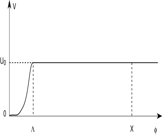
The potential $V_{eff}(X)$ in our class of models can be pictured as a very flat (with logarithmic curvature) plateau at $X\gg\Lambda$. Moreover we know that classically at $X=0$ there are other branches of moduli space. Some of these are supersymmetry preserving even at the quantum level. We expect that the transition between the plateau and these other directions of lower energy takes place smoothly in the region $X{~{}\raise 1.49994pt\hbox{$<$}\kern-8.50006pt\lower 3.50006pt\hbox{$\sim$}~{}}\Lambda$. Physically what happens in this region, is that some mesons or baryons of $G_{S}$ become tachionic and develop a VEV. In the Appendix we discuss this in some more detail for a specific model. In this section we are going to discuss the quantum stability of a false vacuum with these properties. In order to get an estimate of the rate of tunneling we can reduce to a one dimensional potential $V(\phi)$. In some of the cases of interest, the region $\phi<\Lambda$ corresponds to more than one vacuum or flat direction. Still our conclusions are not qualitatively modified in the realistic case. Furthermore in order to make the discussion simpler, we will study the rate of true vacuum bubble nucleation for a truly flat plateau, in the limit in which $\Lambda\ll X$. This is shown in Fig. 1. Indeed, at first sight, this may look like a bad approximation as it eliminates the potential barrier that separates the physically interesting, but false vacuum, from the supersymmetry preserving one. But this is too naive since in field theory the potential energy ${\cal H}$ consists of both a gradient and a static piece

$${\cal H}=\int d^{3}x\left\{(\nabla\phi)^{2}+V(\phi)\right\}.$$ (14)

When the potential $V(\phi)$ is flat, it is the gradient energy $(\nabla\phi)^{2}$ that provides the barrier in the functional space $\{\phi\}$. Consider, indeed, a homogeneous field configuration where $\phi(x)\equiv X$ over all space. Then for any small and local variation $\delta\phi(x)$ of the background field, the static energy is unchanged while the gradient contribution is positive definite

$$\Delta{\cal H}=\Delta{\cal H}_{grad}+\Delta{\cal H}_{stat}=\Delta{\cal H}_{grad}>0.$$ (15)

It is also clear that the larger $X/\Lambda$ the more gradient energy must be generated in order to reach lower potential energy, so the higher the barrier in field space is. We thus expect that for large $X/\Lambda$ the rate of quantum tunneling into the true vacuum will be suppressed. The rate of bubble nucleation can be then evaluated in the semiclassical approximation. This amounts to finding the action for the bounce, a spherically symmetric solution to the Euclidean equations of motion [20]. In terms of the bounce action $S_{B}$, the rate of bubble formation per unit volume $\Gamma/V$ is just given by

$${\Gamma\over V}=\mu^{4}e^{-S_{B}}$$ (16)

where $\mu$ is a mass parameter determined by the calculation of quantum fluctuations around the bounce and which we expect to be of the order of the largest scale in the problem, $X$. The bounce solution $\phi(r)$ satisfies the following boundary conditions and equations of motion

$$\dot{\phi}(0) = \dot{\phi}(\infty)=0\quad\quad\phi(\infty)=X$$ (17)

$$\ddot{\phi} + {3\over r}\dot{\phi}=\partial_{\phi}V(\phi).$$ (18)

The equation of motion describes a classical motion in a one dimensional potential $=-V(\phi)$, with time variable $=r$ and with a friction term whose strength decreases as $1/r$. The particle analogy is very useful and one can apply considerations similar to those made in Ref. [20] for the thin wall bubble. Similar calculations have been done in Refs. [21, 22]. The size of the bubble is simply established by energy conservation. Consider indeed the motion in the plateau region $\phi\geq\Lambda$, see Fig. 1. Here $\phi$ is just a massless field and the solution to eq. (LABEL:eqbounce) is simply

$$\phi(r)=(X-\Lambda)\left[1-\Bigl{(}{R\over r}\Bigr{)}^{2}\right]+\Lambda.$$ (20)

Notice that $\phi(\infty)=X$ and that the radius $R$ is an integration constant characterizing the size of the solution: $\phi(R)=\Lambda$. The kinetic energy $\dot{\phi}^{2}/2$ at $r=R$ is given by $(X-\Lambda)^{2}/2R^{2}\sim X^{2}/2R^{2}$. In view of the presence of a dissipative force, this has to be smaller than the maximum available energy $U_{0}$. Then it must be $R>X/{\sqrt{2}U_{0}}\gg 1/\Lambda$, much bigger than the typical scale of the potential $V(\phi)$. This large radius has two implications: i) as $X/\Lambda\to\infty$ the starting point $\phi(0)\to 0$, where $\partial V=0$, since for $\phi(0)>0$, where $\partial V\sim\Lambda^{3}$, the radius would be too small ${\cal O}(1/\Lambda)$, the only scale in the potential; ii) in the region $\phi<\Lambda$ the friction term are ${\cal O}(1/\Lambda R)$ with respect to the leading terms, so that energy conservation holds up to order $1/R\Lambda{~{}\raise 1.49994pt\hbox{$<$}\kern-8.50006pt\lower 3.50006pt\hbox{$\sim$}~{}}\Lambda/X$. Then from i), ii) and by equating potential and kinetic energy respectively at $\phi\simeq 0$ and $\phi=\Lambda$ we find the bubble radius

$$U_{0}={X^{2}\over 2R^{2}}\left(1+{\cal O}(\Lambda/X)\right)\quad\Longrightarrow\quad R\simeq{X\over{\sqrt{2}U_{0}}}$$ (21)

More qualitatively we can describe the bounce solution as follows. $\phi$ starts very close to the top, and there it stays until friction is small enough to allow the motion to $X\gg\Lambda$. (Remember that in the particle analogy the potential is $-V(\phi)$ of Fig. 1.) At $r\sim R=X/{\sqrt{2U_{0}}}$ the particle goes down the hill. This motion is determined by the fundamental scale $\Lambda$ in $V$ and happens within a thin shell (short time) $\Delta r\sim 1/\Lambda\ll R$. Its contribution to the action is consequently negligible. Indeed we can write the action $S(R)$ as

$$S(R)=-{1\over 2}\pi^{2}U_{0}R^{4}+2\pi^{2}X^{2}R^{2}+{\cal O}(\Lambda^{3}R^{3}).$$ (22)

The first term is from the bulk of the bubble $0<r{~{}\raise 1.49994pt\hbox{$<$}\kern-8.50006pt\lower 3.50006pt\hbox{$\sim$}~{}}R$ where $\phi\sim 0$. The second comes from the massless region $r>R$, where $\phi>\Lambda$, and by using eq. (20). Finally, the third term is an estimate of the contribution from the transition region, the thin shell. By extremizing with respect to $R$ we find the same bounce radius as eq. (21). Neglecting the subleading term we then get the bounce action

$$S_{B}=2\pi^{2}{X^{4}\over U_{0}}\sim 2\pi^{2}\left({X\over\Lambda}\right)^{2}.$$ (23)

The consistency of this approximation can also be verified by noticing that eq. (22) is consistent with the virial theorem $T+2U=0$, where $T,U$ are respectively kinetic and potential energy. This is because the contribution from $r\simeq R$ is all potential while $r>R$ is all kinetic.

Finally with the calculated action we can estimate the lifetime of our universe by using eq. (16). Using the volume of the past light cone we get consistency if $S_{B}>500$. This is easily satisfied, already for $X/\Lambda\sim 10$.

Having established the stability of the vacuum on the plateau at the present, one may ask the same question for the previous stages of evolution of the universe. We do that by “going backward in time”, as later stages of cosmological evolution are obviously more under control. So the first question is: what are the conditions for $X$ not to be driven away by thermal corrections? Intuitively one might expect that at high temperature $T$ a flat direction $X$ with renormalizable interactions is driven to the origin by the positive $\sim T^{2}$ corrections to its mass. However, this is true only for $X{~{}\raise 1.49994pt\hbox{$<$}\kern-8.50006pt\lower 3.50006pt\hbox{$\sim$}~{}}T$, as for $X\gg T$ all the modes coupled to $X$ get heavy and decouple. In these regions the potential is determined by $1/X$ suppressed couplings to the remaining light fields in the Kähler function. This corrections provide a $\sim T^{2}/X$ curvature to the flat direction field. This is negligibly small if the maximum temperature of the universe, namely the reheating temperature, is much smaller than the X. For a reheat temperature $T_{reheat}^{3}<\Lambda^{2}X$ gaugino condensation in the strong group is not affected by the temperature corrections and the zero temperature potential is dominant. Note that for values of $X_{today}$ favoured by our models the above condition is automatically satisfied when $T_{reheat}$ satisfies the gravitino regeneration bound[41]. We conclude that it is consistent to survive in this local minimum during the big bang. The next step behind deals with the evolution of $X$ during inflation. Here, however, the theoretical situation becomes less under control, especially in the absence of a well defined model of inflation.

4 Models

We now illustrate some explicit models built along the ideas of Section 1. We name each of them by its $G_{S}\times G_{B}$ gauge group factor.

4.1   ${\bf SU(2)\times SU(2)_{B1}\times SU(2)_{B2}}$.

The simplest choice for the strong group is $SU(2)$ with a matter content given by four doublets (two flavors) $Q_{I},I=1,\dots,4$. In the massless limit this sector has a global $SU(4)$ flavor symmetry. Any anomaly free subgroup of it may be weakly gauged and play the role of the balancing group $G_{B}$. However we find that the simplest way to realize the requirements of section 1 is to consider $G_{B}=SU(2)\times SU(2)\sim SO(4)\subset SU(4)$. For instance, the smaller subgroups $U(1)$ or $SU(2)$ would not be asymptotically free. The need for asymptotically free balancing group seems to be generic for the mechanism to work.

The matter content under $SU(2)_{S}\times SU(2)_{B1}\times SU(2)_{B2}\times SU(5)$ is

$$Q=(2,2,1,1),\quad\bar{Q}=(2,1,2,1),\quad R=(1,2,2,1),$$

$$q_{3}\oplus q_{2}\oplus q_{1}=(1,1,2,3\oplus 2\oplus 1)\quad\bar{q}_{3}\oplus\bar{q}_{2}\oplus\bar{q}_{1}=(1,2,1,\bar{3}\oplus\bar{2}\oplus\bar{1})$$ (24)

where the $q_{i}$’s have been split into their $SU(3)\times SU(2)\times U(1)$ irreps. Notice that we add a pair of standard model singlets $q_{1},\bar{q}_{1}$ in order to cancel the $SU(2)_{B1}\times SU(2)_{B2}$ global anomaly. The tree superpotential is given by

$$W=R\left(\lambda Q\bar{Q}+\lambda_{3}q_{3}\bar{q}_{3}+\lambda_{2}q_{2}\bar{q}_{2}+\lambda_{1}q_{1}\bar{q}_{1}\right).$$ (25)

The classically flat direction of interest is $X=(detR)^{{1\over 2}}$. Along $X$, we have

$$<R>=X\left(\begin{array}[]{cc}1&0\\ 0&1\end{array}\right)$$ (26)

so that $SU(2)_{B1}\times SU(2)_{B2}$ is broken down to the diagonal $SU(2)_{D}$, and conditions I) and II) of Sect. 2 are satisfied. In the regime in which $SU(2)_{D}$ (and the stardard model gauge group) is weak, the only relevant non-perturbative dynamics is that of $SU(2)_{S}$. (We will later discusss how good this assumption is.) Then, below the scale of $SU(2)_{S}$ confinement, the effective superpotential is $W_{eff}=\lambda X\Lambda^{2}$. The minima of the effective superpotential are determined by the RG evolution of the wave function, as discussed in sect. 2. Let us analyze this model in more detail. Indicating by $\mu$ the renormalization scale we write the RG equations (RGE) in terms of $\tau={1\over 8\pi^{2}}\ln(\mu/M_{\rm Pl})$. Using a vector notation, the gauge $\beta$ functions above the scale $X$ are

$${d\over d\tau}({1\over g_{B}^{2}},{1\over g_{S}^{2}},{1\over g_{3}^{2}},{1\over g_{2}^{2}},{1\over g_{1}^{2}})=(1,4,1,-3,-\frac{43}{5}).$$ (27)

where we have taken $g_{B1}=g_{B2}=g_{B}$, so that the balancing group is $SO(4)$. The equations for $Z_{X}$ and for the Yukawa couplings are

$${d\ln(Z_{X})\over d\tau} = 3g_{B}^{2}-2\bar{\lambda}^{2}-3\bar{\lambda}_{3}^{2}-2\bar{\lambda}_{2}^{2}-\bar{\lambda}_{1}^{2}$$ (28)

$${d\ln\bar{\lambda}^{2}\over d\tau} = 6\bar{\lambda}^{2}+3\bar{\lambda}_{3}^{2}+2\bar{\lambda}_{2}^{2}+\bar{\lambda}_{1}^{2}-6g_{B}^{2}-3g_{S}^{2}$$ (29)

$${d\ln\bar{\lambda}_{3}^{2}\over d\tau} = 2\bar{\lambda}^{2}+7\bar{\lambda}_{3}^{2}+2\bar{\lambda}_{2}^{2}+\bar{\lambda}_{1}^{2}-6g_{B}^{2}-{16\over 3}g_{3}^{2}-\frac{4}{15}g_{1}^{2}$$ (30)

$${d\ln\bar{\lambda}_{2}^{2}\over d\tau} = 2\bar{\lambda}^{2}+3\bar{\lambda}_{3}^{2}+6\bar{\lambda}_{2}^{2}+\bar{\lambda}_{1}^{2}-6g_{B}^{2}-3g_{2}^{2}-\frac{3}{5}g_{1}^{2}$$ (31)

$${d\ln\bar{\lambda}_{1}^{2}\over d\tau} = 2\bar{\lambda}^{2}+3\bar{\lambda}_{3}^{2}+2\bar{\lambda}_{2}^{2}+5\bar{\lambda}_{1}^{2}-6g_{B}^{2}$$ (32)

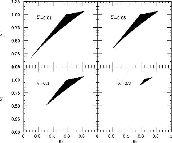
where $\bar{\lambda}_{i}$’s are the running couplings (e.g. $\bar{\lambda}^{2}=\lambda^{2}/(Z_{X}Z_{Q}Z_{\bar{Q}})$). By identifying $\mu$ with $X$, the minima of the potential are given by the solutions to $dZ_{X}/d\tau=0$ with $d^{2}Z_{X}/d\tau^{2}<0$. The quantity $\ddot{Z}_{X}$ is readily computed from eq. (28), with the help of the other RGE. Notice to this effect that the only terms that can make $\ddot{Z}_{X}>0$ are the gauge contributions to the Yukawa RGE. These contributions are indeed big for $\bar{\lambda}^{2}$, and they are sizeable also for $\bar{\lambda}_{2}^{2}$ and $\bar{\lambda}_{3}^{2}$. Therefore for small $\bar{\lambda}_{1}^{2}$, the condition $\ddot{Z}_{X}<0$ cannot be satisfied. On the other hand, when $\bar{\lambda}_{1}^{2}$ is bigger than the other Yukawa couplings, one gets $\ddot{Z}_{X}<0$. Still, in this regime, at a given $X$, $\bar{\lambda}_{1}^{2}$ cannot be made too big, otherwise it hits a Landau pole below $M_{Pl}$. Such considerations determine the regions of parameter space where our mechanism works. In fig. 1 we display, for different values of $\bar{\lambda}$, the region in the plane $(g_{B},\bar{\lambda}_{1})$ for which there is a minimum at $X=10^{10}$ GeV. We have assumed $\bar{\lambda}_{3}=\bar{\lambda}_{2}$ to reduce the number of parameters and because $\bar{\lambda}_{3}\sim\bar{\lambda}_{2}$ is motivated by GUT considerations. The boundaries of the region in the figure are explained as follows: i) the right one is given by $\ddot{Z}_{X}<0$; ii) the top one is essentially dictated by the absence of Landau poles in $\bar{\lambda}_{1}^{2}$ below the Planck scale; iii) the left one is determined by $\bar{\lambda}_{1}^{2}\leq 3g_{B}^{2}$ from $\dot{Z}_{X}=0$, see eq. (28). So it is clear that there is a significant region of parameter space where this model behaves, in the observable MSSM sector, as a conventional gauge mediated supersymmetry breaking model, with messenger scale around $10^{10}$ GeV. We remark that this model shares similarity with an interesting proposal by Izawa and Yanagida [23] and by Intriligator and Thomas [24], where the role of our $R$ is essentially played by a set of gauge singlets. The phenomenological version of that model, mentioned in Ref. [24] and discussed at length in Ref. [3], is unfortunately not calculable. In that model, like in ours, one must live in a local minimum, as the $Q\bar{Q}$ and the $q\bar{q}$ restore supersymmetry at $X=0$. However this local minimum, if it exists, is presumambly at $X{~{}\raise 1.49994pt\hbox{$<$}\kern-8.50006pt\lower 3.50006pt\hbox{$\sim$}~{}}\Lambda$, as the Goldstino superfield $X$ is a gauge singlet and the perturbative superpotential drives it towards the origin (the perturbative corrections to $K(XX^{\dagger})$ were ignored in Ref. [24, 3]). In this region the Kähler potential is not calculable and one has just to assume: 1) the occurrence of such a local minimum; 2) its quantum stability, as there is no obvious parametric suppression of the tunnelling rate at $X\sim\Lambda$.

Figure 2: The region of parameters where the $SU(2)\times SU(2)\times SU(2)$ model can have a local supersymmetry-breaking vacuum at $\langle X\rangle=10^{10}$ GeV.

Around the minimum the real part of $X$ gets a mass

$$m_{X}^{2}=\left({1\over 8\pi^{2}}\right)^{2}\left({\lambda\Lambda^{2}\over X}\right)^{2}{\ddot{Z}_{X}\over 8Z_{X}^{3}}$$ (34)

which is parametrically similar to the sfermion masses in eq. (13). At this stage, the imaginary part of $X$ is the R-axion. Notice that $X$, the axion scale, as far as gauge mediation is concerned, can consistently be in the $10^{9}-10^{12}$ GeV axion window [25]. So $X$ also provides and interesting QCD axion candidate. However there is still the possibility that ${\rm Im}X$ gets a mass from direct sources of explicit $R$ breaking. One of these can arise from the mechanism that cancels the cosmological constant [26]. Another is the $SU(2)_{D}$ anomaly, but this is negligible when the balancing group is weak (see the comments below).

Actually also $SU(2)_{D}$ has a low energy dynamics that leads to an additional term $W_{D}\sim\Lambda_{B}X^{2}$, where $\Lambda_{B}=\Lambda_{1,2}$ is the microscopic strong scale of the balancing $SU(2)$ factors. The combination of the two gaugino condensates restores supersymmetry, as the low energy $W\sim\Lambda^{2}X+\Lambda_{B}X^{2}$ has no effective R-symmetry. However, since we are interested in local minima we are not worried by that, as long as $\Lambda_{B}$ is small enough that the supersymmetry preserving minimum is very distant. This is indeed what happens for the values of $g_{B}(X)$ that are allowed in Fig. 1. Notice that the relative shift in the vev is $\delta X/X\sim 8\pi^{2}\Lambda_{B}/m_{X}$, which for $g_{B}(X)<1$ is less than $10^{-20}$, while another supersymmetry preserving minimum (in addition to those at $X=0$) exists only at $X>M_{Pl}$!

Some more comments are in order. These concern the range of $X$ where the mechanism works. In particular $X$ cannot be too close to $\Lambda$, otherwise our perturbative approximation to the Kähler potential breaks down, due to non-perturbative corrections from the $SU(2)_{S}$ dynamics. Indeed at $X\gg\Lambda$ we expect the non-perturbative corrections to $K(X,X^{\dagger})$, to be dominated by the lowest term in the operator product expansion. This is given by $\int d^{4}\theta(W_{\alpha}^{2})(\bar{W}_{\dot{\alpha}}^{2})/(XX^{\dagger})^{2}$, whose coefficient is $\sim{1\over 8\pi^{2}}$ as it is determined by a 1-loop diagram involving the heavy $Q,\bar{Q}$ and four external vector superfields. After substituting the gaugino condensate the above operator leads to a correction $\delta K(X,X^{\dagger})\sim 8\pi^{2}\Lambda^{4}/(\lambda^{2}XX^{\dagger})$. Thus the effects induced on the Kähler curvature vanish like $(\Lambda/X)^{4}$. Using the above formula for $m_{X}^{2}$, we estimate that this non-perturbative effect can be reasonably neglected for $X{~{}\raise 1.49994pt\hbox{$>$}\kern-8.50006pt\lower 3.50006pt\hbox{$\sim$}~{}}10^{9}$ GeV.

At the other end of the range, for large $X$, operators induced by Planck scale phisics may affect the flatness of the superpotential. We find that, barring the mass term $W=M_{Pl}X^{2}$, the lowest correction $X^{4}/M_{Pl}$ is tolerable when the minimum is at $X{~{}\raise 1.49994pt\hbox{$<$}\kern-8.50006pt\lower 3.50006pt\hbox{$\sim$}~{}}10^{11}$ GeV. For higher messenger scales this term will also have to be suppressed. We notice that while the $X^{2}$ and $X^{4}$ operators are in principle allowed by the symmetries of the model, it is not totally unreasonable to assume they are absent. This is because in supersymmetric theories the absence of a given term in an effective superpotential (now eq. (25) itself) does not necessarily have a symmetry explanation in the low-energy theory. (This is for instance seen in examples of strong gauge dynamics.)

Before concluding we stress that the phenomenology of this model is that of conventional gauge mediation with two families of messengers in the fundamental of $SU(5)$. One could consider generalizations based on $Sp(m)\times Sp(m)\times SU(2m)$, where $m=1$ is just the original model. These work essentially in the same way, but have $2m$ families of messengers.

4.2   ${\bf SU(2n)\times SU(2n)}$ with adjoint matter. Another possibility is to consider $G_{S}=SU(N)_{S}$ and $G_{B}=SU(N)_{B}$, with even $N=2n$ and with the following matter content under $SU(N)_{S}\times SU(2)_{B}\times SU(5)$

$$Q=(N,\bar{N},1),~{}~{}\bar{Q}=(\bar{N},N,1),~{}~{}R=(1,N^{2}-1,1),~{}~{}\bar{q}=(1,N,\bar{5}),~{}~{}q=(1,\bar{N},5).$$ (35)

The classical superpotential is

$$W=\lambda RQ\bar{Q}+\lambda_{5}Rq\bar{q}+{k\over 3}R^{3}.$$ (36)

Again, at the classical level, there is a flat direction along which only $R\not=0$

$$<R>=X\left(\begin{array}[]{cc}1&0\\ 0&-1\end{array}\right)$$ (37)

where the entries represent $n\times n$ blocks. To motivate this choice of model and $W$ we remind that in the absence of a superpotential, there exists an $N-1$ dimensional family of flat directions parametrized by $N-1$ invariants built from $R$: $X_{p}=({\rm Tr}R^{p})^{1/p}$ with $p=2...N$. At a generic point on this vacuum manifold, $SU(N)_{B}$ is broken down to $U(1)^{N-1}$ and there are just $N-1$ massless chiral and $N-1$ massless gauge superfields. There are, however, enhanced symmetry directions (lines) along which a non-Abelian subgroup is unbroken. Here the number of massless gauge and chiral superfields is bigger. A suitable superpotential can lift all but one flat direction. For $SU(mn)$ groups ($m,n$ integers) adding $W={\rm Tr}R^{m+1}$, lifts all moduli but $u_{m}={\rm Tr}R^{m}$, along which $SU(mn)\to SU(n)^{m}$. The special thing about $SU(2n)$ groups is that this job is done by a trilinear invariant ${\rm Tr}R^{3}$. This motivates our choice of even $N$ with $W$ given by eq. (36).

Now, along $X$, see eq. (37), the balancing group is broken down to $SU(n)\times SU(n)$. All other components of $R$ as well as $Q,\bar{Q}$ and $q,\bar{q}$ have a mass of order $X$ and decouple. The low energy dynamics of $SU(N)_{S}$ generates a linear superpotential $W=\lambda X\Lambda^{2}$. One can go through the same analysis we applied to $SU(2)^{3}$. In the models with $N=2n\leq 4$ the balancing group is not asymptotically free, and this makes it impossible to satisfy the minimum condition $\ddot{Z}_{X}<0$. Moreover models with $N\geq 10$ have too many messengers, so that Landau poles in the evolution of the SM gauge coupling are hit before the GUT scale, unless $X$ is very close to $M_{G}$, bringing partially back the supersymmetric flavor problem. We find that a model which works very well over a wide range of scales is $SU(6)\times SU(6)$. Let us discuss it in more detail. The gauge coupling RGE are

$${d\over d\tau}({1\over g_{B}^{2}},{1\over g_{S}^{2}},{1\over g_{3}^{2}},{1\over g_{2}^{2}},{1\over g_{1}^{2}})=(1,12,-3,-7,-{63\over 5}).$$ (38)

The equations for $Z_{X}$ and for the Yukawa couplings are

$${d\ln(Z_{X})\over d\tau} = 12g_{B}^{2}-6\bar{\lambda}^{2}-3\bar{\lambda}_{3}^{2}-2\bar{\lambda}_{2}^{2}-{16\over 3}\bar{k}^{2}$$ (39)

$${d\ln\bar{\lambda}^{2}\over d\tau} = {53\over 3}\bar{\lambda}^{2}+3\bar{\lambda}_{3}^{2}+2\bar{\lambda}_{2}^{2}+{16\over 3}\bar{k}^{2}-{71\over 3}g_{B}^{2}-{35\over 3}g_{S}^{2}$$ (40)

$${d\ln\bar{\lambda}_{3}^{2}\over d\tau} = 6\bar{\lambda}^{2}+{44\over 3}\bar{\lambda}_{3}^{2}+2\bar{\lambda}_{2}^{2}+{16\over 3}\bar{k}^{2}-{71\over 3}g_{B}^{2}-{16\over 3}g_{3}^{2}-\frac{4}{15}g_{1}^{2}$$ (41)

$${d\ln\bar{\lambda}_{2}^{2}\over d\tau} = 6\bar{\lambda}^{2}+3\bar{\lambda}_{3}^{2}+{41\over 3}\bar{\lambda}_{2}^{2}+{16\over 3}\bar{k}^{2}-{71\over 3}g_{B}^{2}-3g_{2}^{2}-\frac{3}{5}g_{1}^{2}$$ (42)

$${d\ln\bar{k}^{2}\over d\tau} = -3{d\ln(Z_{X})\over d\tau}$$ (43)

where again the barred Yukawas indicate running couplings.

Figure 3: The region of parameters where the $SU(6)\times SU(6)$ model can have a local supersymmetry-breaking vacuum at $\langle X\rangle=10^{10}$ GeV.

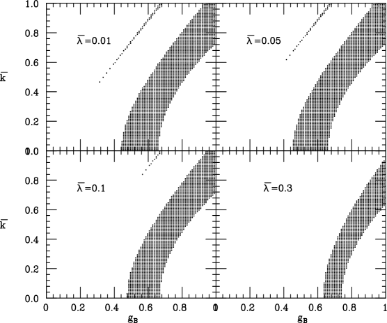
In Fig. 2 we show, for different values of $\bar{\lambda}$ the region in the $(g_{B},\bar{k})$ plane where the model leads to a stable minimum at $X=10^{10}$ GeV. Again we assumed $\bar{\lambda}_{2}=\bar{\lambda}_{3}$. The two disjoint regions arise as follows. The thin region around the line $g_{B}=(2/3)~{}\bar{k}$, corresponds to the points where $\dot{Z}_{X}=0$ is saturated essentially by $\bar{k}$, see eq. (39). To the immediate right of the thin area, $\bar{\lambda}_{2,3}$ are small but non zero. This is enough for the negative contribution of $g_{3}$ and $g_{2}$ to their RGE to make $\ddot{Z}_{X}$ positive. This excludes this intermediate area. However when $\bar{\lambda}_{2,3}$ become large enough, the positive terms in their RGE dominate and $\ddot{Z}_{X}$ becomes negative again. This explains the big allowed band to the right. However as $\bar{\lambda}_{2,3}$ are further increased, they hit a Landau pole below $M_{Pl}$, and the region of large $g_{B}$ is again excluded. The range where the model works becomes even wider as the scale $X$ is increased above $10^{10}$ GeV, as the constraint from Landau poles gets weaker. Also, as for the previous model, the effects on $W$ of the low energy $SU(3)^{2}$ are negligible as soon as $g_{B}(X){~{}\raise 1.49994pt\hbox{$<$}\kern-8.50006pt\lower 3.50006pt\hbox{$\sim$}~{}}1$.

4.3   ${\bf SU(5)^{3}}$. A special model.

As a special case of our general idea one can consider the possibility of identifying $Q,\bar{Q}$ with $q,\bar{q}$. In other words the messengers themselves trigger supersymmetry breaking. This can be achieved in a model with full gauge group $SU(5)_{1}\times SU(5)_{2}\times SU(5)_{3}$ and with matter content given by $R({\bf 1},{\bf 5},{\bf\bar{5}})$, $Q({\bf\bar{5}},1,{\bf 5})$ and $\bar{Q}({\bf 5},{\bf\bar{5}},{\bf 1})$. For phenomenological applications we are interested in a variant (low-energy limit) of this model, one in which $SU(5)_{3}$ is already broken to $SU(3)\times SU(2)\times U(1)$ and the standard matter transforms in $5\oplus\bar{10}$ of $SU(5)_{3}$. To simplify the discussion let us first focus on $SU(5)^{3}$. In view of its role we treat $SU(5)_{3}$ as a weakly gauged factor, and neglect possible effects coming from its non-perturbative dynamics.

The space of $D$-flat directions of the theory is parametrized by 3 baryonic invariants $u={\rm det}(R)$, $v={\rm det}(Q)$, $z={\rm det}(\bar{Q})$ plus a meson $Y=RQ\bar{Q}$. A renormalizable superpotential consists just of the term

$$W=\lambda RQ\bar{Q}=\lambda Y.$$ (45)

This superpotential lifts most flat directions. The classical equations of motion, $\partial_{R}W=0$, $\partial_{Q}W=0$ and $\partial_{\bar{Q}}W=0$, when contracted to form invariants give the constraints

$$uv=uz=vz=0\quad\quad Y=0.$$ (46)

Thus the space of classically flat directions consists of three one-dimensional baryonic branches $u,v,z$ with one common point at the origin. Notice that this result holds also for the model in which one gauge factor, say $SU(5)_{3}$, is not gauged.

The class of models to which this one belongs have been discussed in ref. [27] where it was shown that in the presence of the trilinear superpotential (and treating $SU(5)_{3}$ as weakly gauged) they break supersymmetry at any finite point in field space. Furthermore there is a sloping direction $z\to\infty$ along which the vacuum energy becomes asymptotically zero. However, the dynamics which interests us takes places far away along the $u$ (or $v$ for that matter, since $SU(5)_{1}$ and $SU(5)_{2}$ can be interchanged) flat direction. It is just a special case of the dynamics discussed in Section 2. Along $u$, $R=X\times{\bf 1}$, so that $u=X^{5}$. This breaks the factor $SU(5)_{2}\times SU(5)_{3}$ down to the diagonal $SU(5)_{D}$, which will be later identified with the standard model gauge interactions. Apart from $X$, all the fields in $R,\,Q,\,\bar{Q}$ get mass. Thus the $SU(5)_{1}$ gaugino condensation generates a superpotential $W_{eff}=\Lambda_{L}^{3}=\lambda X\Lambda_{1}^{2}$. A few comments are in order at this point. First of all, this is now an exact result. There are no corrections to it coming from the $SU(5)_{2}$ dynamics. This is not totally surprising, as that group is Higgsed. This result can also be established by studying the global symmetries of the microscopic Lagrangian and using holomorphy. In particular the baryon number $U(1)_{Q}$ with charges $(0,0,1,-1,0,5)$ for $(\lambda,X,Q,\bar{Q},\Lambda_{1}^{10},\Lambda_{2}^{10})$, rules out any dependence of the low energy superpotential on $\Lambda_{2}$.

Now, let us analyze quantitatively the realistic scenario where $SU(5)_{3}\to SU(3)^{\prime}\times SU(2)^{\prime}\times U(1)^{\prime}$. To avoid confusion with gauge group suffixes we rename $SU(5)_{2}\to SU(5)_{B}$ (balancing) and $SU(5)_{1}\to SU(5)_{S}$ (strong). The previous discussion is easily generalized. Now $R\to R_{2}\oplus R_{3}=({\bf 1},{\bf 5},{\bf 2}\oplus{\bf 3})$ and similarly $Q\to Q_{2}+Q_{3}$. The flat direction analysis is unchanged. The vev of $R$ breaks $SU(5)_{B}\times SU(3)^{\prime}\times SU(2)^{\prime}\times U(1)^{\prime}\to SU(3)\times SU(2)\times U(1)$, so that the low energy gauge couplings are

$${1\over g_{i}^{2}(X)}={1\over g_{B}^{2}(X)}+{1\over g_{i}^{\prime 2}(X)}$$ (47)

where the notation is obvious. Notice that at the scale $X$ the gauge couplings $g_{i}$ are modified in an $SU(5)$ invariant manner, so that gauge unification is safe. However, the coupling above $X$ will be somewhat bigger (like $\sqrt{2}$). This we find to be the major source of constraints for this model, as we discuss in more detail below.

The $SU(5)_{1}$ nonperturbative dynamics goes along unmodified. The field $R$ has however broken up into two pieces $R_{2,3}$ whose wave function terms evolve differently and which we indicate by $Z_{X_{2}}$ and $Z_{X_{3}}$. Now, along the flat direction $R_{3}=X_{3}{\bf 1}_{3\times 3}$, $R_{2}=X_{2}{\bf 1}_{2\times 2}$ with $X_{3}/X_{2}=\sqrt{Z_{X_{2}}/Z_{X_{3}}}$ in order to have vanishing $SU(5)_{B}$ D-terms. As before, we parametrize the flat direction with $X^{5}=X_{3}^{3}X_{2}^{2}={\rm det}R$. The Kähler potential along $X$ is now given by

$$K(X,X^{\dagger})=5Z_{X_{2}}^{2\over 5}Z_{X_{3}}^{3\over 5}XX^{\dagger}$$ (48)

so that the minimum condition is

$$5{\dot{Z}_{X}\over Z_{X}}=2{\dot{Z}_{X_{2}}\over Z_{X_{2}}}+3{\dot{Z}_{X_{3}}\over Z_{X_{3}}}=0.$$ (49)

The gauge coupling RGE are

$${d\over d\tau}({1\over g_{B}^{2}},{1\over g_{S}^{2}},{1\over g_{3}^{\prime 2}},{1\over g_{2}^{\prime 2}},{1\over g_{1}^{\prime 2}})=(10,10,-2,-6,-{58\over 5}).$$ (50)

while for the Yukawa couplings we have

$${d\ln(Z_{X})\over d\tau} = {24\over 5}g_{B}^{2}+{3\over 5}g_{2}^{\prime 2}+{8\over 5}g_{3}^{\prime 2}+{1\over 5}g_{1}^{\prime 2}-2\bar{\lambda}_{2}^{2}-3\bar{\lambda}_{3}^{2}$$ (51)

$${d\ln\bar{\lambda}_{3}^{2}\over d\tau} = 13\bar{\lambda}_{3}^{2}+2\bar{\lambda}_{2}^{2}-{48\over 5}g_{B}^{2}-{48\over 5}g_{S}^{2}-{16\over 3}g_{3}^{\prime 2}-{4\over 15}g_{1}^{\prime 2}$$ (52)

$${d\ln\bar{\lambda}_{2}^{2}\over d\tau} = 12\bar{\lambda}_{3}^{2}+2\bar{\lambda}_{3}^{2}-{48\over 5}g_{B}^{2}-{48\over 5}g_{S}^{2}-3g_{2}^{\prime 2}-{3\over 5}g_{1}^{\prime 2}.$$ (53)

This model has no problems with $\ddot{Z}_{X}$ becoming positive. This a consequence of $SU(5)_{B}$ being “strongly” asymptotically free. In a situation like this, the minima in the $1/Z_{X}$ potential are well pronounced. In fact they are so pronounced that the parameter space of this model is strongly constrained by the avoidance of Landau poles in $\bar{\lambda}_{2}^{2},\bar{\lambda}_{3}^{2}$. The constraint is made even more acute by eq. (47), which implies that both $g_{B}^{2}$ and $g_{i}^{\prime 2}$ have to be larger, in practice by about a factor of 2, than the effective $g_{i}^{2}$. This implies that the Yukawas that saturate $\dot{Z}_{X}=0$ have to be rather large too, and their evolution above $X$ quickly reaches a Landau pole. We find that the request of no Landau pole below $10^{17}$ GeV and of perturbative gauge unification sets a lower bound on the scale X

$$X{~{}\raise 1.49994pt\hbox{$>$}\kern-8.50006pt\lower 3.50006pt\hbox{$\sim$}~{}}10^{14}{\rm GeV}$$ (55)

For such an $X$ we find solutions with the following values of the parameters: $g_{B}^{2}(X)\simeq 1-1.2$ and $\bar{\lambda}_{2}^{2}(M_{G})\simeq\bar{\lambda}_{3}^{2}(M_{G})\sim 1.8-3$ and $g_{GUT}^{2}<2$. This is still in the perturbative domain. However, by lowering $X$ we immediately get large Yukawas at the GUT scale. Notice that for $X\sim 10^{15}$ GeV, we start recovering the flavour problem because of gravity contributions to soft masses, thus weakening the motivation for gauge mediated supersymmetry breaking. So we can say that this model works in a fairly limited but still non vanishing range $X\sim 10^{14}-10^{15}$ GeV.

Again we should comment on all additional contributions that may affect the scalar potential. In this model, given the small ratio $\Lambda/X\sim 10^{-5}$, the non-perturbative corrections to the Kähler metric from the $SU(5)_{S}$ dynamics are clearly negligible. But we are very close to the Planck scale. The lowest operator that can affect the flatness is $\delta W={\rm det}X/M_{Pl}^{2}\sim X^{5}/M_{Pl}^{2}$. Then it is clear that for $X\sim 10^{14}$ GeV this correction must be absent, or be very suppressed. If this is the case, flatness is preserved, as the higher order terms like ${\rm detX}^{2}/M_{Pl}^{7}$ are very suppressed. One last source of perturbation can arise from whatever mechanism relaxes to zero the cosmological constant by providing an effectively constant term $\sim\Lambda^{2}M_{Pl}$ in $W$. This term creates in lowest order a linear potential $\delta V\sim\Lambda^{4}{\rm Re}X/M_{Pl}$. This leads to a shift $\delta X$ in the vev of $X$, which is

$${\delta X\over X}\sim(8\pi^{2})^{2}{X\over M_{Pl}}$$ (56)

where the $(8\pi^{2})^{2}$ arises from the expression for $m_{X}^{2}$, see eq. (34). Then again, $X\sim 10^{14}$ GeV is still acceptable, while $X\sim 10^{15}$ GeV starts being problematic. This bound is amusingly similar to the one provided by the flavor problem.

In spite of its very constrained range of validity we think this model is an attractive example of a very elegant way of generating and communicating supersymmetry breaking. Are there any special phenomenological signature of models like this? The answer is in principle yes. Indeed in this theory the messengers of supersymmetry breaking are not exhausted by the chiral superfields $Q,\bar{Q}$. There are also the massive vector superfields in the coset $SU(5)_{B}\times SU(3)^{\prime}\times SU(2)^{\prime}\times U(1)^{\prime}/SU(3)\times SU(2)\times U(1)$. These get a mass from $X$ and feel the effect of $F_{X}\not=0$. A set of these massive vectors transforms as the adjoint of $SU(3)\times SU(2)\times U(1)$ and couples directly to standard matter. We may call these heavy objects the axial gluons, $W$’s and $B$. Indeed already at one loop they affect the sparticle parameters. Since the field $X$ is the only source of infrared cut-off, the form of the correction is fixed by the 1-loop wave function renormalization, as for $K(X,X^{\dagger})$ is Section 2

$$\delta{\cal L}_{soft}\sim\int d^{4}\theta{g_{B}^{2}\over 8\pi^{2}}\ln(XX^{\dagger}/M_{Pl}^{2})QQ^{\dagger}$$ (57)

where the notation is the same as in eq. (12). Notice the interesting fact that this 1-loop correction generates only $A$ terms at order $\alpha/4\pi$. The lowest contribution to the chiral preserving soft masses is zero as $\partial_{X}\partial_{X^{\dagger}}\ln(XX^{\dagger})=0$. Chiral preserving mass squared are generated at ${\cal O}(\alpha^{2})$ by both the above 1-loop operator and by a host of new 2-loop effects. In this way the correct scaling of gaugino and sfermion masses is preserved. This cancellation of dangerous 1-loop effects is the same as the one observed in ref. [28, 29] for the case of standard matter directly coupled to the messengers via Yukawa couplings. We stress once more that in the superfield language the cancellation simply follows from the coincidence of the infrared regulator $X$ and the source of supersymmetry breaking. It does not work, for instance, when the particles in the loop get mass from two independent spurion superfields $X$ and $Y$ for which $X/Y$ is not a c-number. As it was shown in ref. [28, 29] the cancellation works only for the leading contribution in an expansion in powers of $(\Lambda/X)^{2}$. The subleading terms correspond to higher derivative terms in the effective action for $X$ and SM matter, which are not determined by the RG log and for which the above argument does not apply. These higher order effects are however unimportant for this model as $\Lambda/X\ll 1$. A more detailed analysis is needed to determine the effects on the sparticle spectroscopy of the terms induced by the axial vector superfields. It would be interesting to find experimentally important differences. This we leave for further study. One sure thing is that $A$ terms are now induced directly at the messenger scale and they are of the same order as gaugino masses . This may have important implications for the case in which the $\mu$ term in the Higgs sector is provided by a singlet $S$ with couplings $W=S^{3}+SH_{1}H_{2}$. In conventional gauge mediated models the smallness of the RG induced $A$ terms in this sector makes the correct breaking of the electroweak group more difficult. This is the case even when the messenger scale is fairly high. It would be interesting to study the impact of the new boundary conditions.

5 Upper Limits on the Messenger Scale from Nucleosynthesis

The messenger scale is $M$ is constrained by laboratory and astrophysical considerations. The first is the supersymmetric flavor problem, which is a primary motivation for gauge mediated theories. It costrains the messenger scale to be less than about $10^{15}$ GeV [6].

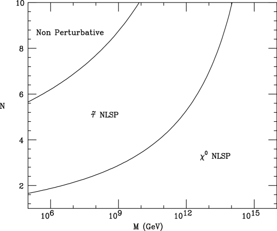
The purpose of this section is to introduce a stronger constraint coming from the requirement that the NLSP decays do not spoil the successful predictions of primordial nucleosynthesis. These constraints will turn out to be fairly independent of the nature of the NLSP which is either a neutralino or the right handed stau depending on the number of messengers $N$ as well as the messenger mass $M$ as shown in fig. 3. Let us first discuss the case when the NLSP is a neutralino, $\chi^{0}$. The decays of $\chi^{0}$ are studied in detail in reference [30]. There it is shown that, in general, the dominant decay modes of $\chi^{0}$ are into a photon and gravitino and, if kinematically allowed, to a lesser extent into $Z^{0}$ and gravitino. The decay rates are given by:

$$\Gamma(\chi^{0}\to\gamma{\tilde{G}})\simeq\cos^{2}\theta_{W}\frac{m_{\chi^{0}}^{5}}{16\pi F^{2}}$$ (58)

$$\Gamma(\chi^{0}\to Z{\tilde{G}})\simeq\sin^{2}\theta_{W}\frac{m_{\chi^{0}}^{5}}{16\pi F^{2}}\left(1-\frac{m_{Z}^{2}}{m_{\chi^{0}}^{2}}\right)^{4}.$$ (59)

The photon of the dominant decay mode can affect nucleosynthesis because it can break-up heavier nuclei into lighter ones [31, 32, 33]. The “damage” that these decays can do to nucleosynthesis depends on the product of the mass of the decaying particle times its abundance relative to baryons (or photons):

$$d_{\gamma}\equiv m_{\chi^{0}}\frac{n_{\chi}}{n_{B}}.$$ (60)

This quantity is somewhat model dependent, as it depends on the sparticle spectrum. For example, the lightest neutralino in typical gauge mediated theories is mostly a B-ino and its abundance relative to baryons depends on its self-annihilation rate and consequently on the slepton spectrum. This in turn depends on $N$ and $M$ and other features of the messenger sector [35]. Nevertheless, the order of magnitude of $d_{\gamma}$ is easy to estimate provided that the typical mass scale of the light supersymmetric particles is about 100 GeV, resulting in a self-annihilation cross section of order $2\pi(\alpha/m)^{2}\simeq 10^{-35}~{}{\rm cm}^{2}~{}m_{100}^{-2}$. Here $m_{100}$ is the typical mass of light sparticles in units of 100 GeV. This yields a mass times abundance per unit entropy [36]:

$$mY_{\infty}\equiv m\frac{n_{X}}{s}\simeq 3\times 10^{-11}~{}{\rm GeV},$$ (61)

corresponding to $d_{\gamma}\sim$ 0.3 $m_{100}$ GeV. This implies that [32, 33] as long as the lifetime of the decaying particle is less than $10^{7}$ sec the damage that the photonic decays can do to nucleosythesis is negligible. They imply an upper limit of the scale of supersymmetry breaking $\sqrt{F}<10^{10}$ GeV or equivalently

$$M<Nm_{100}^{3/2}~{}10^{15}~{}{\rm GeV},$$ (62)

where $N$ is the number of messengers. Therefore we see that the constraint from photodestruction of light elements is quantitatively similar to that from the flavor problem.

Figure 4: The regions in the $N$–$M$ parameter space where the neutralino ($\chi^{0}$) or the right-handed stau (${\tilde{\tau}}$) are the next-to-lightest supersymmetric particle (NLSP). Above the upper curve the gauge coupling constants become non-perturbative before the GUT scale.

A stronger constraint arises from the hadronic decays of $\chi^{0}$ [32]. These occassionally lead to energetic nucleons which subsequently thermalize by colliding with the ambient protons and ⁴He and in the process they create a “hot line” along which a one dimensional version of nucleosynthesis can take place, potentially resulting in overproduction of the light nuclei D, ³He, ⁶Li, ⁷Li [32]. D and ³He arise mostly from “hadrodestruction” – an energetic nucleon breaks up an ambient ⁴He nucleus into ³He or D. ⁷Li and ⁶Li arise from “hadrosynthesis” in which ³He or $T$ or ⁴He are sufficiently activated along the “hot line” to overcome their Coulomb barrier and synthesize ⁶Li or ⁷Li nuclei. The analysis is fairly involved and the reader is referred to reference [34, 32] for the details. The crucial quantity measuring the magnitude of the “damage” of hadronic decays on the primordial nuclear abundances is

$$d_{B}=d_{\gamma}r_{B}^{*},$$ (63)

where $r_{B}^{*}$ is essentially the hadronic branching ratio $r_{B}$ of the decaying particle – it is defined carefully in references [34, 32]. The photon in the decay $\chi^{0}\to\gamma{\tilde{G}}$ can convert to quarks with probability of order $\alpha$, and therefore $r_{B}$ can never be smaller than about $10^{-2}$. The contribution to the hadronic branching ratio from the decay $\chi^{0}\to Z{\tilde{G}}$ is

$$r_{B}\sim 0.7~{}\tan^{2}\theta_{W}~{}\left(1-\frac{m_{Z}^{2}}{m_{\chi^{0}}^{2}}\right)^{4},$$ (64)

where 0.7 is the hadronic branching ratio of the $Z$. This is typically smaller than $10^{-2}$ as long as the $\chi^{0}$ mass is less than about 150 GeV because of phase space suppression. So from now on we take $r_{B}$ to be its minimal value $10^{-2}$; if it is larger then our arguments will get stronger. The value of the corresponding $d_{B}$ is $3\times 10^{-3}$ GeV. From figures 5 of reference [32] we see that even for such a small value of $d_{B}$ the hadronic showers lead to an extreme overproduction of ⁷Li, ⁶Li and D + ³He, if the lifetime of the decaying particle is longer than $10^{4}$ sec. This shows that the lifetime of $\chi^{0}$ must be significantly smaller than $10^{4}$ sec. How short the lifetime has to be before we are safe is not yet known to us. For lifetimes less than $10^{4}$ sec we are not aware of a complete analysis – including the crucial hadronic jets – of the effects of late decays on all the light element abundances, in particular ⁶Li and ⁷Li. One complication is that ordinary nucleosynthesis is occuring simultaneously with the decays. For this reasons it is not possible yet to quote a precise upper limit on the lifetime of a decaying particle from nucleosynthesis. A safe upper limit for the lifetime is about 1 sec, which marks the beginning of nucleosynthesis. This leads to an upper limit of about $10^{8}$ GeV for the scale of supersymmetry breaking $\sqrt{F}$ or,

$$M<Nm_{100}^{3/2}~{}10^{11}~{}{\rm GeV}.$$ (65)

This is a safe upper limit on the messenger scale and is significantly stronger than the limit of $M<10^{15}$ GeV coming from the flavor problem. However, it may be too strict and a detailed analysis may allow for somewhat longer lifetimes [37]. Thankfully, the upper limit on $M$ scales as the square root of the lifetime, so that even if lifetimes of order 100 seconds were allowed they would only increase $M$ by an order of magnitude. This would still lead to an upper limit on M much stronger than the limit coming from the flavor problem. Since most nuclear abundances, in particular that of ⁴He, are in full bloom by the end of 180 seconds we expect that lifetimes longer than 180 seconds are excluded. The point is that the damaging processes of hadrodestruction and hadroproduction – which lead to the overabundances of D+³He and Lithium respectively – rely mainly on the existence of ambient ⁴He which is completely formed by 180 seconds. Furthermore, the universe is sufficiently diluted by 180 seconds that a reduction of the excess abundance is unlikely.

When the NLSP is a right-handed slepton the upper limit to the messenger scale should be even smaller than in eq. (65). The point is that the lightest right handed slepton is the right handed stau which decays into a tau and a Goldstino. Since the tau has a large hadronic branching ratio, the hadronic damage factor $d_{B}$ becomes 0.2 GeV which significantly exceeds that of $\chi^{0}$.

The upper limit in eq. (65) has significant implications on model building. It disfavors theories in which the messenger scale results from the competition between renormalizable and non-renormalizable Planck-supressed operators, since these result in large messenger scales. It favors theories in which the messenger scale is the result of renormalizable competing forces, as is the case here. Even then, it excludes our most favored theory, namely $SU(5)^{3}$.

One, perhaps unappealing, way out of the constraint in eq. (65) is to postulate some degree of $R$-breaking which can result in a microscopic lifetime for the NLSP which is totally decoupled from supersymmetry breaking.

Finally, notice that the longest NLSP lifetime consistent with the flavor problem ($M<10^{15}$ GeV) is $10^{7}$ sec. This implies that the NLSP decays cannot have an effect on the spectrum of the microwave and diffuse background radiation [33, 36].

It is interesting that the nucleosythesis constraint implies that the scale of supersymmetry breaking breaking has to be in the “narrow” range between $10^{4}$ and $10^{8}$ GeV. To avoid the gravitino problem in the high end of this range – between $10^{6}$ and $10^{8}$ GeV – it is necessary that the reheating temperature of the universe be relatively low.

6 Conclusions

Gauge mediated supersymmetry breaking provides a very attractive alternative to gravity mediated scenarios. In gauge mediation the only source of flavor violation which is relevant in low-energy phenomenology is given by the Yukawa matrices of standard quarks and leptons. This leads to the supersymmetric generalization of the GIM mechanism and to the distinctive experimental signature that no major deviation from the SM is expected in flavor and CP violating processes. This is consistent with our present experimental information, and is the main motivation for gauge mediation. The gravity scenario, on the other hand, has a generic difficulty with flavor violation. Nonetheless, the models that can be made consistent with the present bounds (eg. by using horizontal symmetries) still predict that some major deviation from the SM (like $\mu\to e\gamma$ or an electric dipole moment of an elementary particle[40]) will sooner or later be discovered. Whether gravity or gauge interactions mediate soft terms may be answered by accurate low energy experiments.

The breaking of supersymmetry and its mediation (via gauge interactions) at scales much below $M_{Pl}$ should be well described by field theory, with no active role played by quantum gravity. This motivates the study of theories where supersymmetry is broken by some non-perturbative gauge dynamics. This allows for an attractive field theoretic explanation of the smallness of the weak scale itself, not just its quantum stability. It is clear that the discovery of compelling field theory models with dynamically driven and gauge mediated supersymmetry breaking would give this scenario another non-trivial boost over the gravity mediated case.

These facts are at the basis of numerous recent attempts to build realistic theories wedding dynamical SUSY breaking to gauge mediation. The main point of our investigation has been that many of the aesthetic and phenomenological disadvantages of previous attempts are easily avoided by relaxing the request that supersymmetry be broken in the true vacuum. We have characterized a class of theories for which the vacuum where we live is typically a false one, located on a supersymmetry breaking potential energy plateau, far away from from other energetically more favourable minima. This last property can be achieved quite naturally by means of Witten’s inverse hierarchy phenomenon and endows the false vacuum with a lifetime which is much longer than the age of the Universe. This makes it in practice a stable vacuum.

We have characterized a class of calculable theories with a fairly simple structure. The breaking of supersymmetry is communicated to the MSSM sparticles in a minimal number of steps. A measure of this simplicity is the fact that the Goldstino superfield itself gives a mass to the messengers. This is not the case, for instance, in the standard scenario by Dine et al. [2], which contains an additional sector and where the Goldstino is not directly coupled to the messengers. Those models have no supersymmetric ground state, but this does not lead to any clear advantage as the global minimum breaks color and $SU(2)_{W}$ at a high scale. Thus the messenger sector has to live in a local minimum. It seems that in order to have a phenomenologically acceptable true minimum considerable further complication is needed [4]. Notice that these minima are the analog of those that exist in our models, see eq. (1), at $X=0$. Indeed in gauge mediation with a large messenger mass there can yet be other deeper minima along the flat directions $H_{2}=L_{i}$ [38] of the MSSM. This is because in gauge mediation the soft mass $m_{H_{2}}^{2}+m_{\tilde{L}}^{2}$ along this flat direction goes negative very quickly due to the large stop contribution [39]. So it seems that in one way or another gauge mediation brings us the idea that we live in a false vacuum.

Attempts to build theories with just two sectors have flourished in the last year. In particular the models proposed in Ref. [5] ,[6] have a close resemblance to our $SU(5)^{3}$ example. Those models are however phenomenologically non viable, as squarks masses turn out to be negative. This is due to the presence of relatively “light” matter supefields with positive and large supertrace. Since the potential is stabilized by $1/M_{Pl}$ operators, the scale where soft terms (and the supertrace) are generated is fairly large (${~{}\raise 1.49994pt\hbox{$>$}\kern-8.50006pt\lower 3.50006pt\hbox{$\sim$}~{}}10^{15}$ GeV, barely compatible with the flavor problem), the positive suprtrace leads to large and negative squark masses via two loop RG mixing. We stress that our $SU(5)^{3}$ model bypasses the problem by having no such light matter: everything gets a $\sim X$ mass via just one Yukawa coupling. Other new mechanisms were explored in Refs. [7, 8], where the role of $X$ is played by a composite gauge invariant field. Those models, however, involve massive parameters in the superpotential, so they do not yet represent a full microscopic theory.

In previous cases the messenger scale was either fairly low $\sim 10^{5}$ GeV, for renormalizable theories, or fairly high ${~{}\raise 1.49994pt\hbox{$>$}\kern-8.50006pt\lower 3.50006pt\hbox{$\sim$}~{}}10^{15}$, for non-renormalizable ones. In our scenario we have a double dimensional transmutation, one for $F_{X}$ (gaugino condensation) and one for $X$ (Coleman-Weinberg mechanism). By that we can cover the continuum of theories where messengers have a mass that varies from $10^{8-9}$ to $10^{14}$ GeV, and where $10^{6\div 7}{\rm GeV}{~{}\raise 1.49994pt\hbox{$<$}\kern-8.50006pt\lower 3.50006pt\hbox{$\sim$}~{}}F_{X}{~{}\raise 1.49994pt\hbox{$<$}\kern-8.50006pt\lower 3.50006pt\hbox{$\sim$}~{}}10^{9}{\rm GeV}$. Models that live in this intermediate region can more easily avoid the gravitino problem of usual renormalizable models [41] and gravity has no observable flavor effect. Indeed we also pointed out that models with a large messenger scale ${~{}\raise 1.49994pt\hbox{$>$}\kern-8.50006pt\lower 3.50006pt\hbox{$\sim$}~{}}10^{12}$ GeV have serious problems with standard Big Bang nucleosynthesis. This still keeps a large slice of the continuum unconstrained. Models with $X>10^{12}$ GeV, including the otherwise very compelling $SU(5)^{3}$, are in need of additional interactions which allow the NLSP to decay in less than a second. It seems that a possibility would be to add a small source of $R$-parity violation, but with the aesthetic and logical (remember flavor physics) problem that this addition entails. Another totally different way out is to assume a period of GeV scale inflation [42], with GeV scale baryogenesis.

A possible direction for the future is to further enlarge the taxonomy of theories with gauge mediated supersymmetry breaking. For instance, one hope is that with a large pool to choose from, a still unresolved problem like the origin of $\mu$ may be solved in a natural way [28]. Indeed the boundary conditions on soft terms plays a relevant role in this issue, making, for instance the solution by the addition of a singlet $S$ more or less attractive. A crucial aspect is the size of $A$ terms. We have seen that models with heavy vector supefield messengers can lead to a rather different boundary condition with respect to the minimal case, where $A$ terms are generated by gaugino masses via RG evolution.

Note Added

As this paper was about to be submitted a very interesting paper by H. Murayama, hep-ph/9705271, appeared. In that paper a model similar to our $SU(5)^{3}$ is discussed.

Appendix

In this brief Appendix we discuss the dynamics along the flat direction $X$ as the field VEV becames of order $\Lambda$. As an example we choose to illustrate the $SU(5)^{3}$ model, because it is a very attractive one. Nonetheless, in the other cases, the essence of the discussion is the same.

As already said the strong dynamics of $SU(3)^{\prime}\times SU(2)^{\prime}\times U(1)^{\prime}$ can be neglected. The full effective superpotential of the confined $SU(5)_{1}\times SU(5)_{2}$ theory is given by [27]

$$W_{conf}=\lambda{\rm Tr}\hat{Y}+A\left({\rm det}(\hat{Y})-uvz+\Lambda_{1}^{10}u-\Lambda_{2}^{10}v\right)$$ (66)

where $A$ is a Lagrange multiplier enforcing a quantum modified constraint [13]. At least for $\lambda\ll 1$ we expect the above fields and $W_{conf}$ to describe the configurations of lowest energy. Notice that the above superpotential admits no supersymmetric vacua at finite field values. Indeed $F_{Y}=0$ requires $A,Y\not=0$ after which $F_{z}=0$ implies $uv=0$. This last requirement is inconsistent with $F_{u}=F_{v}=0$, unless $z\to\infty$. Far away along $z$ all other baryons and meson are massive, as it is already shown by the classical analysis, and integrating them out yields the effective potential $W_{eff}=(\Lambda_{1}^{2}\Lambda_{2}^{2})/z^{1/5}$ [27]. So supersymmetry is asymptotically recovered only as $z\to\infty$: this theory has no global vacuum. We are however interested in the $u$ branch and in what happens as $X$ is lowered to be $\sim\Lambda_{1}$. In order to so, we first integrate out the meson $Y$ and the field $A$. This is sensible as they are massive over the entire moduli space. As a matter of fact the baryons $u,v,z$ are the only fields that can become very light on some branch of the moduli space. We thus obtain

$$W_{eff}=\lambda\left(uvz+u\Lambda_{1}^{10}-v\Lambda_{2}^{10}\right)^{1\over 5}$$ (67)

The above equations contains all the interesting information regarding the dynamics as we move along $X=(u)^{1/5}$. For $u\not=0$ we can make the reparametrization $\tilde{z}=z-\Lambda_{2}^{10}/u$. Then performing the suitable rescaling of the baryons $v,\tilde{z}$ their mass matrix is roughly given by

$${\cal L}_{mass}=(v^{*},\tilde{z}^{*})\left(\begin{array}[]{cc}\lambda^{2}|X|^{2}&\lambda\Lambda_{1}^{2}\\ \lambda\Lambda_{1}^{2}&\lambda^{2}|X|^{2}\end{array}\right)\left(\begin{array}[]{c}v\\ \tilde{z}\end{array}\right).$$ (68)

where the diagonal terms come from $|F_{v,\tilde{z}}|^{2}$, while the off diagonal from $|F_{X}|^{2}$. At large $X$ the baryons are massive with zero vev, so that by decoupling them we get back the linear $W_{eff}$. However, when $X$ is decreased below some critical value $\sim\Lambda_{1}$ the baryons become tachionic and develop a vev. This indicates that for $X\sim\Lambda_{1}/\lambda$ we enter the basin of attraction of the $z$ flat direction and then slide to infinity. The only point that is crucial for our discussion, however, is that no instability develops for $X{~{}\raise 1.49994pt\hbox{$>$}\kern-8.50006pt\lower 3.50006pt\hbox{$\sim$}~{}}\Lambda_{1}/\lambda$, and thus to tunnel to the asymptotically supersymmetric vacuum the bounce configuration has to interpolate between field values of order $X$ to values of order $\Lambda_{1}/\lambda$.

References

-
[1]
M. Dine, W. Fischler, and M. Srednicki, Nucl. Phys. B189 (1981) 575;
S. Dimopoulos and S. Raby, Nucl. Phys. B192 (1981) 353;
M. Dine and W. Fischler, Phys. Lett. B110 (1982) 227;
M. Dine and M. Srednicki, Nucl. Phys. B202 (1982) 238;
M. Dine and W. Fischler, Nucl. Phys. B204 (1982) 346;
L. Alvarez-Gaumé, M. Claudson, and M. Wise, Nucl. Phys. B207 (1982) 96;
C.R. Nappi and B.A. Ovrut, Phys. Lett. B113 (1982) 175;
S. Dimopoulos and S. Raby, Nucl. Phys. B219 (1983) 479. - [2] M. Dine and A. Nelson, Phys. Rev. D48 (1993) 1277; M. Dine, A. Nelson and Y. Shirman, Phys. Rev. D51 (1995) 1362; M. Dine, A. Nelson, Y. Nir and Y. Shirman, Phys. Rev. D53 (1996) 2658.
- [3] T. Hotta, K.-I. Izawa and T. Yanagida, Phys. Rev. D55 (1997) 415.
- [4] I. Dasgupta, B.A. Dobrescu and L. Randall, Nucl. Phys. B483 (1997) 95.
- [5] E. Poppitz and S. Trivedi, Phys. Rev. D55 (1997) 5508.
- [6] N. Arkadi-Hamed, J. March-Russell, H. Murayama, preprint LBL-39865, hep-ph/9701286.
- [7] L. Randall, preprint MIT-CTP-2591, hep-ph/9612426.
- [8] Y. Shadmi, preprint Fermilab-Pub-97/060-T, hep-ph/9703312.
- [9] M.A. Shifman, A.I. Vainstein, Nucl. Phys. B277 (1986) 456; Nucl. Phys. B359 (1991) 571.
- [10] G. Veneziano and S. Yankielowicz, Phys. Lett. B113 (19,) 82321; T. R. Taylor, G. Veneziano and S. Yankielowicz, Nucl. Phys. B218 (1983) 493.
- [11] V. Novikov, M. Shifman, A. Vainshtein and V. Zakharov, Nucl. Phys. B229 (1983) 381.
- [12] N. Seiberg, Phys. Lett. B318 (1993) 469.
- [13] N. Seiberg, Phys. Rev. D49 (1994) 6857.
- [14] A. Masiero, R.Pettorino, M.Roncadelli, G.Veneziano, Nucl. Phys. B261 (1985) 633-650.
- [15] E. Poppitz and L. Randall, Phys. Lett. B336 (1994) 402.
- [16] E. Witten, Phys. Lett. B105 (1981) 267.
- [17] Y. Shirman, Phys. Lett. B389 (1996) 287.
- [18] L. Alvarez-Gaumé, M. Claudson, and M. Wise, Nucl. Phys. B207 (1982) 96.
- [19] C.D. Carone and H. Murayama, Phys. Rev. D53 (1996) 1658.
- [20] S. Coleman, Phys. Rev. D15 (1977) 2929.
- [21] K. Lee and E.J. Weinberg, Nucl. Phys. B267 (1986) 181; M.J. Duncan and L.G. Jensen, Phys. Lett. B291 (1992) 109.
- [22] A. Kusenko, private communication.
- [23] K.-I. Izawa and T. Yanagida, Prog. Theor. Phys. 95 (1996) 829.
- [24] K. Intriligator and S. Thomas, Nucl. Phys. B473 (1996) 121.
- [25] J. Preskill, M. Wise and F. Wilczek, Phys. Lett. B120 (1983) 127; L. Abbot and P. Sikivie, Phys. Lett. B120 (1983) 133; M. Dine and W. Fischler, Phys. Lett. B120 (1983) 137.
- [26] J. Bagger, E. Poppitz and L. Randall, Nucl. Phys. B426 (1994) 3.
- [27] E. Poppitz, S. Trivedi and Y. Shadmi, Phys. Lett. B388 (1996) 561.
- [28] G. Dvali, G.F. Giudice, and A. Pomarol, Nucl. Phys. B478 (1996) 31.
- [29] M. Dine, Y. Nir, and Y. Shirman, Phys. Rev. D55 (1997) 1501.
[30]
S. Ambrosanio, G.L. Kane, G.D. Kribs, S.P. Martin, and
S. Mrenna, Phys. Rev. D54 (1996) 5395;
S. Dimopoulos, S. Thomas, and J.D. Wells, Nucl. Phys. B488 (1997) 39. -
[31]
D. Lindley, Ap. J. 294 (1985) 1;
J. Ellis, D.V. Nanopoulos, and S. Sarkar, Nucl. Phys. B259 (1985) 175;
R. Dominguez-Tenreiro, Ap. J. 313 (1987) 523;
M.H. Reno and D. Seckel, Phys. Rev. D37 (1988) 3441. - [32] S. Dimopoulos, R. Esmailzadeh, L.J. Hall, and G.D. Starkman, Nucl. Phys. B311 (1989) 699.
- [33] J. Ellis, G.B. Gelmini, J.L. Lopez, D.V. Nanopoulos, and S. Sarkar, Nucl. Phys. B373 (1992) 399.
- [34] S. Dimopoulos, R. Esmailzadeh, L.J. Hall, and G.D. Starkman, Ap. J. 330 (1988) 545.
- [35] S. Dimopoulos and G.F. Giudice, Phys. Lett. B393 (1997) 72.
- [36] E.W. Kolb and M.S. Turner, The Early Universe, Addison-Wesley Pub., 1990.
- [37] S. Dimopoulos, L. Krauss, and G. Starkman, work in progress.
- [38] H. Komatsu, Phys. Lett. B215 (1988) 323.
- [39] P. Ciafaloni and A. Strumia, preprint UAM-FT-403, hep-ph/9611204; R. Rattazzi and U. Sarid, preprint CERN-TH/96-349, hep-ph/9612464.
- [40] L.J. Hall, V.A. Kostelecky and S. Raby, Nucl. Phys. B267 (1986) 415; R. Barbieri and L.J. Hall, Phys. Lett. B338 (1994) 212.
- [41] A. de Gouvêa, T. Moroi and H. Murayama, preprint LBNL-39753, hep-ph/9701244.
- [42] S. Dimopoulos and L.J. Hall, Phys. Lett. B196 (1987) 135.