Solving the Bethe-Salpeter equation for bound states of scalar
theories in Minkowski space

Abstract

We apply the perturbation theory integral representation (PTIR) to solve for the bound state Bethe-Salpeter (BS) vertex for an arbitrary scattering kernel, without the need for any Wick rotation. The results derived are applicable to any scalar field theory (without derivative coupling). It is shown that solving directly for the BS vertex, rather than the BS amplitude, has several major advantages, notably its relative simplicity and superior numerical accuracy. In order to illustrate the generality of the approach we obtain numerical solutions using this formalism for a number of scattering kernels, including cases where the Wick rotation is not possible.

I Introduction

We present here an improved approach to the solution of the scalar-scalar Bethe-Salpeter (BS) equation directly in Minkowski space, utilising the Perturbation Theory Integral Representation (PTIR) of Nakanishi [6]. The PTIR is a generalised spectral representation for $n$-point Green’s functions in Quantum Field Theory.

This work extends and improves earlier work which applied the PTIR approach to the BS amplitude [1]. Here we formulate a real integral equation for the BS vertex. This considerably simplifies the expression for the kernel function relative to those obtained for the BS amplitude [1]. In particular, some singularity structures which were present in the kernel of the BS amplitude equation due to the constituent particle propagators are absent in the corresponding expression for the BS vertex. Consequently, it is much simpler to implement the problem numerically, and we therefore do not encounter previous difficulties with residual numerical noise. We have checked that our numerical results are in agreement with those obtained in Euclidean space by other authors (for example, Linden and Mitter [9], or more recently, Nieuwenhuis and Tjon [10, 11]). In particular, with sufficient computer time we have seen no limit to the accuracy that can be achieved with our formalism. We can routinely obtain four figure accuracy on a workstation.

In this work we will deal exclusively with scalar theories. For simplicity we will consider here bound states with equal-mass constituents, although it is easy, and desirable in many applications, to generalise the approach to unequal-mass constituents.

We illustrate the BS equation for a scalar theory in Fig. 1, where $\Phi(p,P)$ is the BS amplitude, $P\equiv p_{1}+p_{2}$ is the total four-momentum of the bound state and $p\equiv\eta_{2}p_{1}-\eta_{1}p_{2}$ is the relative four-momentum for the two scalar constituents. We have then $M=\sqrt{P^{2}}$ for the bound state mass and also $\eta_{1}+\eta_{2}=1$, but otherwise the choice of the two positive real numbers $\eta_{1}$ and $\eta_{2}$ is arbitrary. As in Ref. [1] we choose here $\eta_{1}=\eta_{2}$=1/2.

The renormalised constituent scalar propagators are $D(p_{1,2}^{2})$ and $K(p,q;P)$ is the renormalised scattering kernel. For example, in simple ladder approximation in a $\phi^{2}\sigma$ model we would have $K(p,q;P)=(ig)(iD_{\sigma}([p-q]^{2}))(ig)$, where $D_{\sigma}(p^{2})=1/(p^{2}-m_{\sigma}^{2}+i\epsilon)$ and $m_{\sigma}$ is the $\sigma$-particle mass. Note that the corresponding proper (i.e, one-particle irreducible) vertex for the bound state is related to the BS amplitude by $\Phi=(iD)(i\Gamma)(iD)$.

We follow standard conventions in our definitions of quantities, (see Ref. [3, 4] and also, e.g., [5]). Thus the BS equation for any scalar theory can be written as

$$i\Gamma(p_{1},p_{2})=\int{d^{4}q\over(2\pi)^{4}}(iD(q_{1}^{2}))~{}(i\Gamma(q_{1},q_{2}))~{}(iD(q_{2}^{2}))~{}K(p,q;P)\,,$$ (1)

where similarly to $p_{1}$ and $p_{2}$ we have defined $q_{1}=\eta_{1}P+q$ and $q_{2}=\eta_{2}P-q$. Equivalently in terms of the BS amplitude we can write

$$D(p_{1}^{2})^{-1}~{}\Phi(p,P)~{}D(p_{2}^{2})^{-1} = -\int{d^{4}q\over(2\pi)^{4}}~{}\Phi(q,P)~{}K(p,q;P)$$ (2)

$$\equiv ~{}\int{d^{4}q\over(2\pi)^{4}i}~{}\Phi(q,P)~{}I(p,q;P)\,,$$ (3)

where the kernel function defined by $I(p,q;P)\equiv-iK(p,q;P)$ is the form typically used by Nakanishi [2]. In ladder approximation for a $\phi^{2}\sigma$ model we see for example that $I(p,q;P)=g^{2}/(m_{\sigma}^{2}-(p-q)^{2}-i\epsilon)$. In this treatment we will solve the vertex version of the BS equation, i.e. Eq. (1), for an arbitrary scattering kernel.

II PTIR for Scalar Theories

In contrast to the approach in Ref. [1], we will begin with the Bethe-Salpeter equation for the bound-state vertex, Eq. (1), rather than the equivalent equation for the amplitude, Eq. (3), and derive a real integral equation for the BS vertex. To do this we require spectral representations for the vertex, for the $\phi$ propagator, and for the scattering kernel $I$ of Eq. (1). The renormalised $\phi$ propagator may be written as

$$D(q)=-\left({1\over m^{2}-q^{2}-i\epsilon}+\int_{(m+\mu)^{2}}^{\infty}d\alpha\frac{\rho_{\phi}(\alpha)}{\alpha-q^{2}-i\epsilon}\right),$$ (4)

where $\rho_{\phi}(\alpha)$ is the renormalised spectral function. Note that $\rho_{\phi}(\alpha)\geq 0$, (see, e.g., Ref [3]).

The Bethe-Salpeter amplitude $\Phi(p,P)$ for the bound state of two $\phi$-particles having the total momentum $P\equiv p_{1}+p_{2}$ and relative momentum $p\equiv(\eta_{2}p_{1}-\eta_{1}p_{2})$ can be defined as

$$\langle 0|T\phi(x_{1})\phi(x_{2})|P\rangle=e^{-iP\cdot X}\langle 0|T\phi(\eta_{2}x)\phi(-\eta_{1}x)|P\rangle=e^{-iP\cdot X}\int{d^{4}p\over(2\pi)^{4}}e^{-ip\cdot x}\Phi(p,P)\;,$$ (5)

where the fields for the scalar constituents are denoted by $\phi$, and where we have made use of the translational invariance of the BS amplitude. Following the conventions of Itzykson and Zuber [4] (e.g., pp. 481-487), we define centre-of-momentum and relative coordinates $X\equiv\eta_{1}x_{1}+\eta_{2}x_{2}$ and $x\equiv x_{1}-x_{2}$ such that $x_{1}=X+\eta_{2}x$, $x_{2}=X-\eta_{1}x$, and $P\cdot X+p\cdot x=p_{1}\cdot x_{1}+p_{2}\cdot x_{2}$.

Equivalently to Eq.(5), we can write

$$\Phi(p,P)=e^{iP\cdot X}\int d^{4}xe^{ip\cdot x}\langle 0|T\phi(x_{1})\phi(x_{2})|P\rangle=\int d^{4}xe^{ip\cdot x}\langle 0|T\phi(\eta_{2}x)\phi(-\eta_{1}x)|P\rangle\;.$$ (6)

Note that the bound states are normalised such that $\langle P|P^{\prime}\rangle=2\omega_{P}(2\pi)^{3}\delta^{3}(\vec{P}^{\prime}-\vec{P})$, where $\omega_{P}\equiv({\vec{P}}^{2}+M^{2})^{1/2}$ with $M$ the bound state mass. For a positive energy bound state we must have $P^{2}=M^{2}$, $0<P^{2}\leq(2m)^{2}$, and $P^{0}>0$. The normalization condition for the BS amplitude is given by

$$\int\frac{d^{4}p}{(2\pi)^{4}}\int\frac{d^{4}q}{(2\pi)^{4}}\bar{\Phi}(q,P)\frac{\partial}{\partial P_{\mu}}\left\{D^{-1}(p_{1}^{2})D^{-1}(p_{2}^{2})(2\pi)^{4}\delta^{4}(p-q)+K(p,q;P)\right\}\Phi(p,P)=2iP^{\mu}\;,$$ (7)

where the conjugate BS amplitude $\bar{\Phi}(p,P)$ is defined by

$$\bar{\Phi}(p,P)=e^{-iP\cdot X}\int d^{4}xe^{-ip\cdot x}\langle P|T\phi^{\dagger}(x_{1})\phi^{\dagger}(x_{2})|0\rangle=\int d^{4}xe^{-ip\cdot x}\langle P|T\phi^{\dagger}(\eta_{2}x)\phi^{\dagger}(-\eta_{1}x)|0\rangle\;.$$ (8)

A PTIR for Scattering Kernel

The scattering kernel $I(p,q;P)\equiv-iK(p,q;P)$ describes the process $\phi\phi\rightarrow\phi\phi$, where $p$ and $q$ are the initial and final relative momenta respectively. It is given by the infinite series of Feynman diagrams which are two-particle irreducible with respect to the initial and final pairs of constituent $\phi$ particles. For purely scalar theories without derivative coupling we have the formal expression for the full renormalised scattering kernel [6]

$$I(p,q;P) = \int\limits_{0}^{\infty}d\gamma\int\limits_{\Omega}d\vec{\xi}\left\{\frac{\rho_{st}(\gamma,\vec{\xi})}{\gamma-\left[\sum_{i=1}^{4}\xi_{i}q_{i}^{2}+\xi_{5}s+\xi_{6}t\right]-i\epsilon}\right.+\frac{\rho_{tu}(\gamma,\vec{\xi})}{\gamma-\left[\sum_{i=1}^{4}\xi_{i}q_{i}^{2}+\xi_{5}t+\xi_{6}u\right]-i\epsilon}$$ (10)

$$\left.+\frac{\rho_{us}(\gamma,\vec{\xi})}{\gamma-\left[\sum_{i=1}^{4}\xi_{i}q_{i}^{2}+\xi_{5}u+\xi_{6}s\right]-i\epsilon}\right\}\;,$$

where $q_{i}^{2}$ is the 4-momentum squared carried by $\phi_{i}$ and $s$,$t$ and $u$ are the usual Mandelstam variables. The symbol $\Omega$ denotes the integral region of $\xi_{i}$ such that $\Omega\equiv\{\xi_{i}\,|\,0\leq\xi_{i}\leq 1,\,\sum\xi_{i}=1\,(i=1,\dots,6)\}$. The scattering kernel PTIR can be re-written in a more compact form as

$$I(p,q;P) = \sum_{\rm ch}\int\limits_{0}^{\infty}d\gamma\int\limits_{\Omega}d\vec{\xi}\frac{\rho_{\rm ch}(\gamma,\vec{\xi})}{\gamma-(a_{\rm ch}q^{2}+b_{\rm ch}p.q+c_{\rm ch}p^{2}+d_{\rm ch}P^{2}+e_{\rm ch}q.P+f_{\rm ch}p.P)-i\epsilon},$$ (11)

where the subscript “ch” indicates which channel we are dealing with (either $st$, $tu$ or $us$), and {$a_{\rm ch},\ldots,f_{\rm ch}$} are linear combinations of the $\xi_{i}$ (see Appendix B).

For more general theories involving, e.g., fermions and/or derivative couplings, the numerator of Eq. (10) will also contain momenta in general. Work is in progress to extend the formalism to include cases, such as derivative coupling and fermions, where momentum dependence exists in the numerator.

To illustrate our approach we will present here results for three choices of kernel:
(a) Scalar-scalar ladder model with massive scalar exchange: The simple $t$-channel one-$\sigma$-exchange kernel is given by

$$I(p,q;P)=\frac{g^{2}}{m_{\sigma}^{2}-(p-q)^{2}-i\epsilon}$$ (12)

The BS equation with this kernel together with the perturbative constituent particle propagator $D^{0}$ is often referred to as the “scalar-scalar ladder model”[2]. Note that the kernel weight function is proportional to $g^{2}$ for this simple case.
(b) Dressed ladder model: In this instance we dress the propagator of the exchanged $\sigma$ of case (a). The kernel then consists of the pole term as above, plus a piece which involves an integration (starting at a threshold of $4m^{2}$) over a mass parameter $\gamma$.
(c) Generalised kernel: A sum of the one-$\sigma$-exchange kernel Eq. (12) and a generalised kernel with fixed kernel parameter sets $\{\gamma^{(i)},\vec{\xi}^{(i)}\}$. After the Wick rotation this kernel becomes complex due to the $p\cdot P$ and $q\cdot P$ terms, so that solving the BS amplitude as a function of Euclidean relative momentum would be very difficult in this case.

The Wick rotated BS equation for cases (a) and (b) has been studied numerically[9]. We use the previous numerical results for these kernels as a check of our new technique and numerical calculations.

B PTIR for BS vertex

As in Ref. [1], we will use the following form of the $s$-wave ($\ell=0$) BS vertex:

$$\Gamma(p,P)=\int\limits_{0}^{\infty}d\alpha\int\limits_{-1}^{1}dz\frac{\rho_{n}(\alpha,z)}{\left[m^{2}+\alpha-\left(p^{2}+zp\cdot P+\frac{P^{2}}{4}\right)-i\epsilon\right]^{n}}\;,$$ (13)

with the following boundary condition for the weight function:

$$\lim_{\alpha\rightarrow\infty}\frac{\rho_{n}(\alpha,z)}{\alpha^{n-1}}=0\;,$$ (14)

required to render the $\alpha$–integral finite. A partial integration of Eq.(13) with respect to $\alpha$ will serve to demonstrate that the positive integer $n$ is a dummy parameter, since it follows from such a step that weight functions associated with successive values of $n$ are connected by the following relation:

$$\rho_{n+1}(\alpha,z)=n\int\limits_{0}^{\alpha}d\alpha^{\prime}\rho_{n}(\alpha^{\prime},z)\;.$$ (15)

Note that the larger the dummy integer parameter $n$, the smoother the corresponding weight function. This is a particularly useful observation since we have a numerical solution of the BS equation in mind.

Using the same arguments as outlined in [1], it can be shown that the vertex PTIR for bound states with non-zero angular momentum $\ell$ in an arbitrary frame of reference is

$$\Gamma^{[\ell,\ell_{z}]}(p,P)={\cal Y}_{\ell}^{\ell_{z}}(\vec{p^{\prime}})\int\limits_{0}^{\infty}d\alpha\int\limits_{-1}^{1}dz\frac{\rho^{[\ell]}_{n}(\alpha,z)}{\left[m^{2}+\alpha-\left(p^{2}+zp\cdot P+P^{2}/4\right)-i\epsilon\right]^{n}}\;,$$ (16)

where $P$ is an arbitrary timelike 4-vector with $P^{2}=M^{2}$ and $p^{\prime}=\Lambda^{-1}(P)p$. The Lorentz transformation $\Lambda(P)$ connects $P$ and the bound-state rest frame 4-vector $P^{\prime}=(M,\vec{0})$, i.e, $P=\Lambda(P)P^{\prime}$. The quantity ${\cal Y}_{\ell}^{\ell_{z}}(\vec{p^{\prime}})$ is the solid harmonic of order $\ell$, and may be written in the form $|\vec{p^{\prime}}|^{\ell}Y_{\ell}^{\ell_{z}}(\hat{p}^{\prime})$, where $Y_{\ell}^{\ell_{z}}$ is the ordinary spherical harmonic of order $\ell$, $\hat{p}^{\prime}\equiv\vec{p^{\prime}}/|\vec{p^{\prime}}|$, and where $\vec{p^{\prime}}$ is the 3-vector relative momentum in the bound state rest frame. It is relatively straightforward to appreciate why Eq. (16) must be the correct form for a scalar bound state with angular momentum $\ell$. It follows from the self-reproducing property of the solid harmonics (see Eq. (C15) in Appendix C) and from the fact that in the bound state rest frame $\vec{p^{\prime}}$ is the only available three-vector.

In the following sections we will study the BS equation Eq. (1) in an arbitrary frame in terms of this integral representation. Note that the dummy parameter $n$ can always be taken sufficiently large such that the loop-momentum integral of the BS equation, Eq. (1), converges for any $\ell$ for which a bound state exists.

Before proceeding, we should address the issue of so-called ghost states. A bound state whose BS amplitude $\Phi(p,P)$ and equivalent vertex $\Gamma(p,P)$ are anti–symmetric under the transformation $P\cdot p\rightarrow-P\cdot p$ with fixed $p^{2}$ and $P^{2}$ has a negative norm and is called a “ghost”[2]. This symmetry corresponds to the one: $\bar{z}\rightarrow-\bar{z}$ in PTIR form. We do not consider such states herein, as they are unphysical.

III BS Equation for the Weight Function

In this section we will reformulate the BS equation Eq. (1) as an integral equation in terms of the weight functions. This is the central result of this paper. We will very briefly describe the procedure, and state our main results; the details of the derivation may be found in Appendix C, as may definitions of the kernel and associated functions.

We proceed by combining, using Feynman parametrisation, the integral representations for the scattering kernel and vertex with the bare propagators for the constituent $\phi$ particles. The procedure can easily be generalised to include dressed constituent propagators if desired, but we do not exercise this option here, for the sake of simplicity. After using the PTIR representations for the BS kernel and vertex (i.e., Eqs. (11) and (16)) in the right-hand side of the BS equation (Eq. (1)), and after performing Feynman parametrisation for the right-hand side, the BS equation can be written as

$$\Gamma^{[\ell,\ell_{z}]}(p,P) = {\cal Y}_{\ell}^{\ell_{z}}\int\limits_{-\infty}^{\infty}d\bar{\alpha}\int\limits_{-1}^{1}d\bar{z}\frac{1}{[F(\bar{\alpha},\bar{z};p,P)-i\epsilon]^{n}}$$ (17)

$$\times \int\limits_{0}^{\infty}d\alpha\int\limits_{-1}^{1}dz\frac{\rho_{n}^{[\ell]}(\alpha,z)}{\alpha^{n}}\;\bar{\alpha}^{n}[\lambda\;{}^{\rm tot}\!{\cal K}_{n}^{[\ell]}(\bar{\alpha},\bar{z};\alpha,z)],$$ (18)

where $F(\alpha,z;p,P)\equiv m^{2}+\alpha-(q^{2}+zp\cdot P+\frac{1}{4}P^{2})$ is a convenient shorthand notation. We have defined an “eigenvalue” $\lambda\equiv g^{2}/(4\pi)^{2}$, which we will use in our numerical work (see Appendix A). This has simply been factored out of the scattering kernel for convenience and for ease of comparison with other calculations in the ladder limit. The total kernel function ${}^{\rm tot}\!{\cal K}_{n}^{[\ell]}$ is defined in Appendix C (see Eqs. (C46) and (C50)) and its structure is discussed in Appendix D with particualr attention paid to any potential singularities.

Comparing Eq. (18) with Eq. (16), and using the uniqueness theorem of PTIR[6], we finally obtain the following integral equation for $\rho^{[\ell]}_{n}(\alpha,z)$:

$$\frac{1}{\lambda}\frac{\rho^{[\ell]}_{n}(\bar{\alpha},\bar{z})}{\bar{\alpha}^{n}}=\int\limits_{0}^{\infty}d\alpha\int\limits_{-1}^{1}dz\,{}^{\rm tot}\!{\cal K}^{[\ell]}_{n}(\bar{\alpha},\bar{z};\alpha,z)\frac{\rho^{[\ell]}_{n}(\alpha,z)}{\alpha^{n}}.$$ (19)

This equation is the central result of this work. Note that in Eq.(19) we are solving for $\rho_{n}^{[\ell]}/\alpha^{n}$; this is for reasons of convenience for our numerical treatment of the BS equation.

Summary: Since the weight functions $\rho_{\rm ch}(\gamma,\vec{\xi})$ for the scattering kernel are real functions by their construction, the total kernel function ${}^{\rm tot}\!{\cal K}^{[\ell]}_{n}(\bar{\alpha},\bar{z};\alpha,z)$ is real, so that Eq. (19) is a real integral equation in two variables $\alpha$ and $z$. Thus we have transformed the BS equation, which is a singular integral equation of complex distributions, into a real integral equation which is frame-independent. Once one solves for the BS vertex weight function, the BS vertex and the BS amplitude can be written down in an arbitrary frame. This is clearly advantageous for applications of the BS amplitude to relativistic problems.

IV Numerical Results

In this section we present numerical solutions for the BS vertex for bound states in scalar theories using Eq.(19) for three simple choices of scattering kernel:
(a) pure ladder kernel with massive scalar exchange,
(b) dressed ladder kernel with pole term as in (a), and
(c) a generalised kernel combined with the pure ladder kernel of (a).

The scattering kernel (a), i.e., the one-$\sigma$-exchange kernel depending only on $t=(p-q)^{2}$, is given by Eq.(12). This corresponds to choosing for the kernel in Eq. (10) say: $\rho_{tu}=\rho_{us}=0$ and in the $st$-channel $\gamma=m_{\sigma}^{2}$, and $a_{st}=c_{st}=1$, $b_{st}=-2$, $d_{st}=e_{st}=f_{st}=0$, [c.f., Eq. (11)], which amounts to choosing $\rho_{st}$ to be an appropriate product of $\delta$-functions multiplied by $g^{2}$. In the pure ladder case it is convenient (and traditional) to factorise out the coupling constant $g^{2}$ and a factor of $(4\pi)^{2}$, by defining the “eigenvalue” $\lambda=g^{2}/(4\pi)^{2}$ [7, 8, 9]. Thus it is usual to fix the bound state mass $P^{2}$ and then to solve for the coupling $g^{2}$, which is what we have done here.

In general (and for example, for the dressed ladder kernel) the kernel depends on higher powers of the coupling than $g^{2}$; in such instances we update the running value of $\lambda$ in an appropriate way during the iteration process (see Appendix A).

Since the BSE is a homogeneous integral equation and we are only interested at present in extracting the coupling at fixed bound state mass, the choice of normalisation is unimportant provided that it is fixed in some reasonable way.

The numerical solution of the vertex BSE is performed by choosing a suitable grid of $\alpha$ and $z$ values, making an initial guess for the vertex weight function, and then iterating the integral equation (19) to covergence. One subtle point is that integrable square-root singularities may occur and must be appropriately handled numerically (see Appendices A and D for details). By optimising the choice of grid and increasing the number of grid points it was straightforward to increase the accuracy of the solutions to a relative error of 1 part in 10⁴ and beyond. Further details of the numerical procedure used are given in Appendix A.

A Pure Ladder Kernel

We have solved the vertex BS equation, Eq.(19), for a number of bound state masses between $P^{2}=0$ (Goldstone-like bound state) and $P^{2}=4m^{2}$ (the stability threshold). Solutions were obtained for orbital excitations up to $\ell=4$ with no difficulties. We plot some examples of our solutions for $\ell=0$ and $\ell=1$ in Fig. 2, and tabulate our results for the “eigenvalue” $\lambda\equiv g^{2}/(4\pi)^{2}$ in Table I. A plot of the spectrum for $\ell=0$, i.e., of $\lambda$ vs. the fraction of binding $\eta\equiv\sqrt{P^{2}}/2m$, is given in Fig. 3. All solutions presented were obtained using a $\sigma$ mass of $m_{\sigma}=m/2$. We have compared our eigenvalues to those obtained in the Wick-rotated treatment of Linden and Mitter [9], and have found agreement to better than 0.03% for moderate choices of the ($\alpha,z$)-grid. This is an improvement in accuracy of at least one order of magnitude over the results we have obtained previously for the BS amplitude. Furthermore, much greater accuracy is possible through an increase in the number of grid points used in the numerical integration should it be desired for whatever reason.

B Dressed Ladder Kernel

For the “dressed ladder” case, the scattering kernel is given by $I=-iK=(ig)D_{\sigma}(ig)$, where $D_{\sigma}$ is the renormalised $\sigma$-propagator at one-loop order. This is simply the sum of the pole term, Eq.(12), and a continuum part, and is given by

$$D_{\sigma}[(p-q)^{2}]=\int\limits_{0}^{\infty}ds\frac{\rho_{\sigma}(s)}{s-(p-q)^{2}-i\epsilon},$$ (20)

where $\rho_{\sigma}(s)$=$\rho_{\rm pole}(s)+\rho_{\rm cont}(s)$. $\rho_{\rm pole}(s)$ is simply $\delta(s-m_{\sigma}^{2})$, and it can be shown that, to one-loop order, $\rho_{\rm cont}(s)$ is given by the following expression:

$$\rho_{\rm cont}=\lambda\theta(s-4m^{2})\sqrt{\frac{s-4m^{2}}{s}}\frac{1}{\Delta(s)},$$ (21)

where $\Delta(s)$ is the following function:

$$\Delta(s) = \left[m_{\sigma}^{2}-s-\lambda\left\{2\sqrt{\frac{4m^{2}-m_{\sigma}^{2}}{m_{\sigma}^{2}}}\arctan\sqrt{\frac{m_{\sigma}^{2}}{4m^{2}-m_{\sigma}^{2}}}\right.\right.$$ (24)

$$\qquad+\left.\left.\frac{4(m_{\sigma}^{2}-s)}{m_{\sigma}^{2}}\left(\frac{m^{2}}{\sqrt{m_{\sigma}^{2}(4m^{2}-m_{\sigma}^{2})}}\arctan\sqrt{\frac{m_{\sigma}^{2}}{4m^{2}-m_{\sigma}^{2}}}-\frac{1}{4}\right)\right.\right.$$

$$\qquad\qquad+\left.\left.2\sqrt{\frac{s-4m^{2}}{s}}\ln\left(\frac{\sqrt{s}+\sqrt{s-4m^{2}}}{2}\right)\right\}\right]^{2}$$

$$+ \lambda^{2}\pi^{2}\left(\frac{s-4m^{2}}{s}\right).$$ (25)

Note that the use of Eq. (20) introduces an extra integration (over the mass parameter $s$). We performed this numerically using gaussian quadrature; 10 to 15 quadrature points in $s$ provide solutions of satisfactory accuracy.

We have solved Eq. (19) for the dressed ladder kernel above, with the pole being situated at $m_{\sigma}=m$, for various values of the bound state mass squared, $P^{2}$. As for the pure ladder case above, solutions have been obtained up to $\ell=4$. For example, our $s$-wave ($\ell=0$) eigenvalue for $P^{2}=3.24m^{2}$ and for the exchange particle pole at $m_{\sigma}=m$ is $\lambda=1.516$ for a grid of $80\times 41$ and is $\lambda=1.518$ for a grid of $150\times 91$. The corresponding Linden and Mitter value is $\lambda_{E}=1.518$. Even with a relatively coarse grid high accuracies result. Similarly, we have found for other values of $P^{2}$ that an accuracy of 0.3% or better is routinely attained, even with the use of the coarse $80\times 41$ grid. As the above results demonstrate higher accuracy is easily obtained at the cost of more CPU time.

We plot the re-scaled weight function, $\rho_{2}^{[0]}/\alpha^{2}$, for the case $P^{2}=0.04m^{2}$ in Fig. 4 for purposes of comparison with the corresponding ladder case. We have chosen this value of $P^{2}$ since a smaller bound-state mass corresponds to tighter binding and hence larger coupling, which should enhance the effect of this one-loop self-energy insertion. We see that the shape of the weight function is not qualitatively very different from the ladder case.

C Generalised Kernel

This particular example of a “generalised” kernel is an instance of a scattering kernel for which Euclidean space solution is not possible. We have solved the BS equation for this case, in particular for a sum of the pure ladder kernel as described above and two randomly chosen non-ladder terms, each with a weight of $0.25\lambda$, and with the following fixed parameter sets (in the $st$ channel):

$$\{\gamma,a_{st},b_{st},c_{st},d_{st},e_{st},f_{st}\}=$$ (26)

$$(1) \{2.25m^{2},0.47261150181,-0.29743163287,0.58277042955,$$ (28)

$$0.28282145969,-0.23965580016,0.32196629047\}$$

$$(2) \{2.25m^{2},0.47261150181,0.29743163287,0.58277042955,$$ (30)

$$0.28282145969,-0.23965580016,-0.32196629047\}.$$

The parameters $\{a_{st},\ldots,f_{st}\}$ were obtained from a set of values $\{\xi_{1},\ldots,\xi_{6}\}$ produced by a random number generator (see Appendix B). This was done to emphasise that our technique produces well-behaved solutions for an arbitrary kernel. We have had little difficulty obtaining noise-free solutions for this kernel for orbital excitations up to $\ell=4$.

This kernel yields an $s$-wave eigenvalue of $\lambda\equiv g^{2}/(4\pi)^{2}=1.3569$ for $P^{2}=1.44m^{2}$, c.f. the ladder value of $\lambda=1.9402$ for the same bound state mass. We therefore find, as before [1], that the additions to the pure ladder kernel have enhanced the binding, i.e. they are attractive. This is of course to be expected in a scalar theory and was also observed in Refs. [10, 11]. Not only is the eigenvalue lower, but additional structure is present in the vertex weight function (see Fig. 5). In contrast to the solutions obtained for the BS amplitude in the previous work [1], we find that there is no numerical noise in the vertex weight function. If one compares the general kernel example solution in Fig. 5 with the ladder solution for the same bound-state mass (see Fig. 2), it is readily apparent that there is some additional structure superimposed upon the weight function, due to the addition of the generalised kernel terms.

V Summary and Conclusions

We have derived a real integral equation for the weight function of the scalar-scalar Bethe-Salpeter (BS) vertex from the BS equation for scalar theories without derivative coupling. This was achieved using the perturbation theory integral representation (PTIR), which is an extension of the spectral representation for two-point Green’s functions, for both the scattering kernel [Eq. (10)] and the BS vertex itself [Eq. (16)]. The uniqueness theorem of the PTIR and the appropriate application of Feynman parametrisation then led to the central result of the paper given in Eq. (19).

We have demonstrated that Eq.(19) is numerically tractable for several simple kernels, including a randomly chosen case where it is not possible to write the kernel as a sum of ordinary Feynman diagrams. Our results for both the pure and dressed ladder kernels are in excellent agreement with the results obtained previously in the Wick-rotated approach. The agreement for the pure ladder kernel is even better than in Ref. [1], vindicating our decision to solve here the vertex equation rather than the amplitude equation. We obtained an accuracy in all of our results of approximately 1 in 10⁴ with modest ($\alpha,z$)-grid choices on a workstation. This can be improved by using finer grids and larger computers as desired.

Further applications of our formalism are currently being investigated, particularly the crossed ladder and separable kernels. These will not only provide yet another test of our implementation of the method, as Euclidean space results are also available for these cases, but also will provide us with an opportunity to solve a problem featuring more realistic scattering kernels.

It is also important to consider how the PTIR can be extended to include fermions and derivative coupling, so that we have a covariant framework within which to study, for example, mesons in QCD using a coupled Bethe-Salpeter—Dyson-Schwinger equation approach. This would require us to incorporate confinement into the PTIR, which at this stage remains another important and interesting challenge.

[Those interested in applications of this technique may request a copy of the computer code from AGW at the given e-mail address.]

A Algorithm

Here we detail the algorithm used in our numerical studies of the integral equation:

$$\frac{1}{\lambda}\frac{\rho_{n}^{[\ell]}(\bar{\alpha},\bar{z})}{\bar{\alpha}^{n}}=\int\limits_{0}^{\infty}d\alpha\int\limits_{-1}^{1}dz\;\frac{\rho_{n}^{[\ell]}(\alpha,z)}{\alpha^{n}}\;{}^{\rm tot}\!{\cal K}_{n}^{[\ell]}(\bar{\alpha},\bar{z};\alpha,z;\lambda).$$ (A1)

where we have explicitly shown the coupling dependence of the kernel function. We have defined here an “eigenvalue” $\lambda\equiv g^{2}/(4\pi)^{2}$. Our rationale for this is as follows: for a given scattering kernel the integral equation (A1) may be solved for the bound state mass $P^{2}=M^{2}$. However, the dependence of the kernel function ${}^{\rm tot}\!{\cal K}_{n}^{[\ell]}(\bar{\alpha},\bar{z};\alpha,z)$ on the bound state mass $P^{2}$ is highly non–linear and complicated. It is therefore convenient and traditional to instead solve the equation for the coupling $g^{2}$, which appears in the weight function $\rho_{\rm ch}(\gamma,\vec{\xi})$ for the scattering kernel, with a fixed bound state mass $P^{2}$. We first fix the bound state mass $P^{2}$ and regard the integral equation (A1) as an “eigenvalue” problem. The “eigenvalue” is then introduced by factorising the coupling constant $g^{2}$ from the scattering kernel weight function $\rho_{\rm ch}(\gamma,\vec{\xi})$. In this convention, the kernel function ${}^{\rm tot}\!{\cal K}_{n}^{[\ell]}(\bar{\alpha},\bar{z};\alpha,z;\lambda)$ becomes a power series in $\lambda$ starting from ${\cal O}(1)$ for a perturbative scattering kernel.

Strictly speaking, the integral equation (A1) is not an “eigenvalue” equation, since the kernel function itself contains $\lambda$ in the general (i.e., non-ladder) case. We thus solve the equation by iteration rather than applying methods for eigensystems. With an appropriate initial guess for the weight function $\rho_{n}^{[\ell]}(\alpha,z)$ for the BS vertex and the coupling constant $\lambda$ we generate the new weight function by evaluating the RHS of the integral equation (A1). The “eigenvalue” $\lambda$ associated with the weight function is extracted by imposing an appropriate normalization condition which we will discuss later. This generated weight function and its “eigenvalue” are used as inputs and we obtain updated values, which ought to be closer to the solution than the input values, by evaluating the integral. We repeat this cycle until both the “eigenvalue” and the weight function converge.

The normalization condition for the BS vertex or equivalent BS amplitude in momentum space is well known and involves the derivative of the scattering kernel with respect to the bound state 4-momentum $P$ (See Eq.(7) in Sec.II). When the scattering kernel depends on the total momentum $P$, the normalization condition is the integral over two relative momenta; one for the BS vertex and the other for the conjugate one. The corresponding normalization condition in PTIR form is written as the 4-dimensional integral over spectral parameters $\alpha$ and $z$. Imposing a condition that involves such a multi–dimensional integral in the iteration cycle makes the calculation less accurate and time consuming. We shall rather use a suitable normalization condition for the weight function $\rho_{n}^{[\ell]}(\alpha,z)$ during the iteration. The physical normalization condition (7) may be imposed by appropriately rescaling the obtained solution. Of course, the value of $\lambda\equiv g^{2}/(4\pi)^{2}$ is unaffected by the choice of normalisation of the vertex weight function.

Since we are considering bound states whose constituents are of equal mass $m$, we expect that a physically reasonable scattering kernel $I(p,q;P)$ will give a kernel function ${\cal K}_{n}^{[\ell]}(\bar{\alpha},\bar{z};\alpha,z;\lambda)$ symmetric under the transformation $\bar{z}\rightarrow-\bar{z}$. The weight function $\rho_{n}^{[\ell]}(\alpha,z)$ is then either symmetric or anti–symmetric in $z\rightarrow-z$. For a symmetric solution the following normalization is convenient:

$$\int\limits_{0}^{\infty}d\alpha\int\limits_{-1}^{1}dz\;\frac{\rho_{n}^{[\ell]}(\alpha,z)}{\alpha^{n}}=1,$$ (A2)

provided that the integral does not identically vanish. From Eq. (C46), the kernel function is given by the difference of two terms, viz ${\cal K}_{n}^{[\ell]}(\bar{\alpha},\bar{z};0,0;\lambda)-{\cal K}_{n}^{[\ell]}(\bar{\alpha},\bar{z};\alpha,z;\lambda)$. With the normalization condition (A2) the integral equation (A1) can be written as an inhomogeneous one:

$$\frac{1}{\lambda}\;\frac{\rho_{n}^{[\ell]}(\bar{\alpha},\bar{z})}{\bar{\alpha}^{n}}={\cal K}_{n}^{[\ell]}(\bar{\alpha},\bar{z};0,0;\lambda)-\int\limits_{0}^{\infty}d\alpha\int\limits_{-1}^{1}dz\;\frac{\rho_{n}^{[\ell]}(\alpha,z)}{\alpha^{n}}\;{\cal K}_{n}^{[\ell]}(\bar{\alpha},\bar{z};\alpha,z;\lambda).$$ (A3)

On the other hand, the integral of the weight function over $\alpha$ and $z$ for an anti–symmetric solution vanishes identically. Then the integral equation (A1) is written as

$$\frac{1}{\lambda}\frac{\rho_{n}^{[\ell]}(\bar{\alpha},\bar{z})}{\bar{\alpha}^{n}}=-\int\limits_{0}^{\infty}d\alpha\int\limits_{-1}^{1}dz\;\frac{\rho_{n}^{[\ell]}(\alpha,z)}{\alpha^{n}}\;{\cal K}_{n}^{[\ell]}(\bar{\alpha},\bar{z};\alpha,z;\lambda).$$ (A4)

As discussed in the main text, the bound state whose BS amplitude $\Phi(p,P)$ and equivalent vertex $\Gamma(p,P)$ are anti–symmetric under the transformation $P\cdot p\rightarrow-P\cdot p$ with fixed $p^{2}$ and $P^{2}$ has a negative norm and is called a “ghost”[2]. This symmetry corresponds to the one: $\bar{z}\rightarrow-\bar{z}$ in PTIR form. Thus a bound state whose weight function is anti–symmetric in $z$–reflection and which satisfies the homogeneous integral equation (A4) is a “ghost” state. We hereafter concentrate on the “normal” solutions, namely $z$–symmetric ones, and on the integral equation (A3).

It can be shown that the inhomogeneous term vanish unless $\bar{\alpha}>\alpha_{\rm th}$, where $\alpha_{\rm th}$ is the threshold of the weight function depending on the value of $\bar{z}$ for a given scattering kernel. For a one–$\sigma$ exchange kernel with the mass $\mu$, the threshold can be written as

$$\alpha_{\rm th}(\bar{z})=\left(\left(m^{2}-(1-\bar{z}^{2})\frac{P^{2}}{4}\right)^{1/2}+\mu\right)^{2}-\left(m^{2}-(1-\bar{z}^{2})\frac{P^{2}}{4}\right)$$ (A5)

This threshold determines the support of the weight function $\rho$ or equivalently $\varphi$ for the normal solution. Although we cannot write the threshold in a simple form like (A5) for general scattering kernels, we can extract it numerically by analyzing the inhomogeneous term. On the other hand, the kernel function ${\cal K}_{n}^{[\ell]}(\bar{\alpha},\bar{z};\alpha,z;\lambda)$ has the support property for a given $\bar{\alpha}$, $\bar{z}$ and $z$ that it vanishes unless $\alpha$ is less than some value $\alpha_{\rm max}$. For the case of a one–$\sigma$ exchange kernel it is given by

$$\alpha_{\rm max}(\bar{\alpha},\bar{z},z) = \left(\left(\bar{\alpha}+\left(m^{2}-(1-\bar{z}^{2})\frac{P^{2}}{4}\right)^{1/2}-\mu\right)^{2}-\left(m^{2}-(1-\bar{z}^{2})\frac{P^{2}}{4}\right)\right)\frac{1\mp z}{1\mp\bar{z}},$$ (A7)

$$\qquad\qquad\qquad\qquad\qquad\qquad\qquad\qquad\qquad\qquad\qquad\qquad\qquad\qquad\hbox{for }\bar{z}\mathrel{\hbox to0.0pt{\lower 3.0pt\hbox{$<$}\hss}\raise 3.0pt\hbox{$>$}}z.$$

As in the case of $\alpha_{\rm min}$ the analytic form of the upper limit $\alpha_{\rm max}$ is unknown, so we extract the corresponding upper limit numerically for general scattering kernels. Writing these limits of the integral explicitly the integral equation we use is then

$$\frac{1}{\lambda}\;\frac{\rho_{n}^{[\ell]}(\bar{\alpha},\bar{z})}{\bar{\alpha}^{n}}={\cal K}_{n}^{[\ell]}(\bar{\alpha},\bar{z};0,0;\lambda)-\int\limits_{-1}^{1}dz\int_{\alpha_{\rm th}(z)}^{\alpha_{\rm max}(\bar{\alpha},\bar{z},z)}d\alpha\;\frac{\rho_{n}^{[\ell]}(\alpha,z)}{\alpha^{n}}\;{\cal K}_{n}^{[\ell]}(\bar{\alpha},\bar{z};\alpha,z;\lambda).$$ (A8)

We evaluate the integral over $\alpha$ and $z$ in the RHS of Eq. (A8) as follows. Recall that the kernel function ${\cal K}_{n}^{[\ell]}(\bar{\alpha},\bar{z};\alpha,z;\lambda)$ is given by the following integral:

$${\cal K}_{n}^{[\ell]}(\bar{\alpha},\bar{z};\alpha,z;\lambda)\equiv\sum_{\rm ch}\int\limits_{\Omega}d\vec{\xi}\int\limits_{0}^{\infty}d\gamma\;\left[\frac{1}{g^{2}}\rho_{\rm ch}(\gamma,\vec{\xi})\right]K_{n}^{[\ell]}(\bar{\alpha},\bar{z};\alpha,z;\gamma,\vec{\xi})\;.$$ (A9)

We thus start by replacing the integrations over Feynman parameters $\vec{\xi}$ and the spectral variable $\gamma$ by summations over discretised variables. Secondly, we map the semidefinite range of $\alpha\in[0,\infty)$ to the finite one $y\in[0,1]$:

$$\alpha=\alpha_{0}+C\frac{y}{1-y},$$ (A10)

where $\alpha_{0}$ and $C$ are some constants which should be chosen such that the weight function is largest around the mapped variable $y\sim 1/2$. We then discretise both $y$ (equivalently $\alpha$) and $z$ and prepare the initial weight function on this grid. For each cycle of the iteration we perform the integral as follows. We first evaluate the $\alpha$ integral for a given point in the $\bar{\alpha}$ and $\bar{z}$ plane and on the $z$ grid. For each value of the discretised $\vec{\xi}$ and $\gamma$ we extract the support of the the kernel function $K_{n}^{[\ell]}(\bar{\alpha},\bar{z};\alpha,z;\lambda)$. We then divide the integral range $[\alpha_{\rm th}(z),\alpha_{\rm max}(\bar{\alpha},\bar{z},z)]$ into subranges according to the support of the kernel function with discretised $\vec{\xi}$ and $\gamma$. As discussed in Appendix D the kernel function $K_{n}^{[\ell]}(\bar{\alpha},\bar{z};\alpha,z;\lambda)$ may diverge as an integrable square root singularity at the boundary of the support. While this is always the case for the one $\sigma$ exchange kernel, the kernel may take a finite value in general. We thus choose an appropriate integration method to perform the integration over $\alpha$ for each subrange. The weight function at arbitrary $\alpha$ is evaluated by interpolating the values of $\rho$ on the grid. We perform the $\alpha$ integral in this way for each grid point of $z$ and the integral over $z$ is performed by interpolating these values. With this careful treatment of integrable square root singularities we need not introduce any regularization or cutoff parameters. Furthermore, this method allows us to choose the $\bar{\alpha}$ and $\bar{z}$ grid for the newly generated weight function independent of the $\alpha$ and $z$ grid. We optimise the “new” grid by analyzing the shape of the “old” weight function used in the RHS of Eq.(A8). The eigenvalue is evaluated using the normalization condition (A2).

B PTIR for Scattering Kernel

In this appendix we list the dimensionless coefficients $\{a_{\rm ch},b_{\rm ch},c_{\rm ch},\dots,f_{\rm ch}\}$ in Eq. (11) for different channels $\{{\rm ch}\}=\{{st}\},\{{tu}\},\{{us}\}$ in terms of the Feynman parameters $\xi_{i}$ defined in Eq. (10).

	$st$	$tu$	$us$
$\quad a_{\rm ch}\quad$	$\xi_{1}+\xi_{2}+\xi_{6}$	$\xi_{1}+\xi_{2}+\xi_{5}+\xi_{6}$	$\xi_{1}+\xi_{2}+\xi_{5}$
$b_{\rm ch}$	$-2\xi_{6}$	$2(\xi_{6}-\xi_{5})$	$2\xi_{5}$
$c_{\rm ch}$	$\xi_{3}+\xi_{4}+\xi_{6}$	$\xi_{3}+\xi_{4}+\xi_{5}+\xi_{6}$	$\xi_{3}+\xi_{4}+\xi_{5}$
$d_{\rm ch}$	$\quad{1\over 4}(\xi_{1}+\xi_{2}+\xi_{3}+\xi_{4})+\xi_{5}\quad$	$\quad{1\over 4}(\xi_{1}+\xi_{2}+\xi_{3}+\xi_{4})\quad$	$\quad{1\over 4}(\xi_{1}+\xi_{2}+\xi_{3}+\xi_{4})+\xi_{6}\quad$
$e_{\rm ch}$	$\xi_{1}-\xi_{2}$	$\xi_{1}-\xi_{2}$	$\xi_{1}-\xi_{2}$
$f_{\rm ch}$	$\xi_{3}-\xi_{4}$	$\xi_{3}-\xi_{4}$	$\xi_{3}-\xi_{4}$

Beginning with the above definitions for the scattering kernel parameters in terms of the Feynman parameters $\vec{\xi}$, and noting that $\sum_{i=1}^{6}\xi_{i}=1$, it is possible to prove the following relations between the kernel parameters, for all three channels:

$$ac-\frac{b^{2}}{4} \geq 0$$ (B1)

$$\left|f\pm\frac{b}{2}\right| \leq c$$ (B2)

$$\left|af-\frac{eb}{2}\right| \leq ac-\frac{b^{2}}{4}.$$ (B3)

C Kernel Function

In this appendix we detail our derivation of the real integral equation for the BS vertex. We begin with the following PTIR form of the bound-state vertex [7]:

$$\Gamma^{[\ell,\ell_{z}]}(q,P)={\cal Y}_{\ell}^{\ell_{z}}(\Lambda^{-1}(P)q)\int\limits_{0}^{\infty}d\alpha\int\limits_{-1}^{1}dz\frac{\rho_{n}^{[\ell]}(\alpha,z)}{[F(\alpha,z;q,P)-i\epsilon]^{n}}.$$ (C1)

In Eq. (C1), ${\cal Y}_{\ell}^{\ell_{z}}(\Lambda^{-1}(P)q)$ is the solid harmonic for a bound state with angular momentum quantum numbers $\ell$ and $\ell_{z}$, $\rho_{n}^{[\ell]}(\alpha,z)$ is the PTIR weight function for the bound state vertex function, and $n$ is a dummy parameter. The function $F$ is given by

$$F(\alpha,z;q,P) = \alpha+\frac{1+z}{2}(m^{2}-(q+{\textstyle\frac{1}{2}}P)^{2})+\frac{1-z}{2}(m^{2}-(-q+{\textstyle\frac{1}{2}}P)^{2})$$ (C2)

$$= \alpha+m^{2}-(q^{2}+zq\cdot P+{\textstyle\frac{1}{4}}P^{2}).$$ (C3)

We proceed by substituting this form of the vertex into the vertex BSE, Eq. (1), and combining the various factors on the right hand side of the resultant equation (bare propagators, scattering kernel and vertex PTIR) using Feynman parametrisation. We first combine the bare propagators for the scalar constituents with the denominator of the vertex PTIR:

$$D(q+{\textstyle\frac{1}{2}}P)D(-q+{\textstyle\frac{1}{2}}P)\frac{1}{[F(\alpha,z;q,P)-i\epsilon]^{n}}$$ (C4)

$$= \frac{1}{2}\frac{\Gamma(n+2)}{\Gamma(n)\Gamma(2)}\int\limits_{-1}^{1}d\eta\int\limits_{0}^{1}dt\;t^{n-1}(1-t)\frac{1}{[F(t\alpha,tz+(1-t)\eta;q,P)-i\epsilon]^{n+2}}.$$ (C5)

We now combine the factor $1/[F(\ldots)]^{n+2}$ from the integrand with the denominator of the PTIR for the scattering kernel (see Eq. (11)). After some algebra this yields

$$\frac{1}{\gamma-(aq^{2}+bp\cdot q+cp^{2}+dP^{2}+eq\cdot P+fp\cdot P)-i\epsilon}\frac{1}{[F(t\alpha,tz+(1-t)\eta;q,P)-i\epsilon]^{n+2}}$$ (C6)

$$= \frac{\Gamma(n+3)}{\Gamma(1)\Gamma(n+2)}\int\limits_{0}^{1}dx\;\frac{x^{n+1}}{(1-x)^{n+3}}\frac{1}{(y+a)^{n+3}}$$ (C7)

$$\times \frac{1}{[\{[c(y+a)-(b^{2}/4)]/(y+a)^{2}\}F^{\prime}-\{q+[bp+(e+[tz+(1-t)\eta]z)P]/2(a+y)\}^{2}-i\epsilon]^{n+3}},$$ (C8)

where

$$F^{\prime} \equiv F[{\cal A}(t\alpha,tz+(1-t)\eta;y),{\cal Z}(tz+(1-t)\eta;y);p,P],$$ (C9)

$${\cal A}(\alpha,z;y) \equiv \frac{1}{c(y+a)-\frac{b^{2}}{4}}\Biggl{[}\left\{\alpha+m^{2}-(1-z^{2})\frac{P^{2}}{4}\right\}(y+a)^{2}$$ (C10)

$$+ \left\{\gamma-(a+c)m^{2}-a\alpha+(a+c-4d+2z(e-az))\frac{P^{2}}{4}\right\}(y+a)$$ (C11)

$$+ \frac{b^{2}}{4}\left\{m^{2}-\left(1-\left(\frac{-2(az-e)}{b}\right)^{2}\right)\frac{P^{2}}{4}\right\}\Biggr{]}$$ (C12)

$${\cal Z}(z;y) \equiv \frac{f(y+a)-\frac{b}{2}(e+yz)}{c(y+a)-\frac{b^{2}}{4}}$$ (C13)

$$y \equiv \frac{x}{1-x}.$$ (C14)

Note that the parameters $\{a,\ldots,f\}$ do not explicitly have the subscript “ch” attached to them in this instance (cf. Appendix B and Eq. (10)), for the sake of brevity. We will also, for the time being, omit for brevity the sum over channels $st$, $tu$, $us$ in the kernel function.

Having combined all factors on the right hand side, we are now in a position to perform the integral over the loop momentum $q$. To do so, we must utilise the following property of the solid harmonics,

$$\int\limits d^{3}q{\cal F}(\vec{q}\,^{2}){\cal Y}_{\ell}^{\ell_{z}}(\vec{q}+\vec{p})={\cal Y}_{\ell}^{\ell_{z}}(\vec{p})\int\limits d^{3}q{\cal F}(\vec{q}\,^{2}),$$ (C15)

where $F$ is a sufficiently rapidly decreasing function which gives a finite integral [7]. Also note that $\Lambda^{-1}(P)$ boosts the 4-vector $P$ to rest, i.e. $\Lambda^{-1}(P)P=(\sqrt{P^{2}},\vec{0})$, and that the solid harmonics are functions purely of the three-vector part of their argument, i.e. ${\cal Y}_{\ell}^{\ell_{z}}(p)=|\vec{p}\/|^{\ell}Y_{\ell}^{\ell_{z}}(\hat{p})$ (here $\hat{p}=\vec{p}/|\vec{p}\/|$). Bearing this in mind, we obtain for the loop integral

$$\int\limits\frac{d^{4}q}{(2\pi)^{4}i}\frac{{\cal Y}_{\ell}^{\ell_{z}}(\Lambda^{-1}(P)q)}{\left[\widetilde{M}^{2}-\left(q+\frac{bp+(e+zy)P}{2(a+y)}\right)^{2}-i\epsilon\right]^{n+3}}$$ (C16)

$$= \left(-\frac{b}{2}\right)^{\ell}\frac{1}{(a+y)^{\ell}}\frac{\Gamma(n+1)}{(4\pi)^{2}\Gamma(n+3)}\frac{{\cal Y}_{\ell}^{\ell_{z}}(\Lambda^{-1}(P)p)}{(\widetilde{M}^{2}-i\epsilon)^{n+1}},$$ (C17)

where $\widetilde{M}^{2}$ is simply that part of the denominator of Eq. (C8) that does not depend at all on the 4-momentum $q$.

Ignoring integrations over weight functions for the moment, we have, after performing the loop momentum integral, the following result:

$$\int\limits\frac{d^{4}q}{(2\pi)^{4}i}I(p,q;P)D(q+{\textstyle\frac{1}{2}}P)D(-q+{\textstyle\frac{1}{2}}P)\frac{{\cal Y}_{\ell}^{\ell_{z}}(\Lambda^{-1}(P)q)}{[F(\alpha,z;q,P)-i\epsilon]^{n}}$$ (C18)

$$= \frac{1}{(4\pi)^{2}}\frac{1}{2}\left(-\frac{b}{2}\right)^{\ell}\frac{\Gamma(n+1)}{\Gamma(n)}$$ (C19)

$$\times \hskip 14.22636pt\int\limits_{-1}^{1}d\eta\int\limits_{0}^{1}dt\;t^{n-1}(1-t)\int\limits_{0}^{1}dx\frac{1}{(1-x)^{2}}\frac{y^{n+1}}{(y+a)^{\ell}}\frac{(y+a)^{n-1}}{[c(y+a)-\frac{b^{2}}{4}]^{n+1}}$$ (C20)

$$\times \hskip 42.67912pt\frac{{\cal Y}_{\ell}^{\ell_{z}}(\Lambda^{-1}(P)p)}{\left[F({\cal A}(t\alpha,tz+(1-t)\eta;y),{\cal Z}(tz+(1-t)\eta;y);p,P)-i\epsilon\right]^{n+1}}.$$ (C21)

In order to obtain a real integral equation involving only weight functions, it is necessary to recast the last factor in Eq. (C21) in a form similar to that found in the vertex PTIR, Eq. (C1). To proceed we therefore insert the trivial integral

$$\int\limits_{-1}^{1}d\bar{z}\;\delta\left(\bar{z}-{\cal Z}(tz+(1-t)\eta;y)\right)=1$$ (C22)

into the right-hand side of (C21), and eliminate the integration over $t$ by rewriting the delta function in terms of $t$. We are permitted to do this because the function ${\cal Z}$ is bounded between -1 and 1. That this is true is easily seen by observing that ${\cal Z}$ is monotonic in the variable $y$, with $y\in[0,\infty)$, and then by taking the limits $y\rightarrow 0$ and $y\rightarrow\infty$. The former limit gives

$${\cal Z}(z;y\rightarrow 0)=\frac{af-\frac{eb}{2}}{ac-\frac{b^{2}}{4}},$$ (C23)

and so from the third inequality in Eq. (B3) we have that $|{\cal Z}(z;y\rightarrow 0)|\leq 1$. The second limit gives

$${\cal Z}(z;y\rightarrow\infty)=\frac{f-\frac{b}{2}z}{c},$$ (C24)

which allows us to use the second inequality in Eq. (B3) to conclude that $|{\cal Z}(z;y\rightarrow\infty)|\leq 1$, given that (C24) is monotonic in $z$. Since $|{\cal Z}|\leq 1$ in these two limits, ${\cal Z}$ must be bounded between $-1$ and 1 for all $y\in[0,\infty)$.

The insertion of this integral gives us

$$\frac{1}{(4\pi)^{2}}\frac{1}{2}\left(-\frac{b}{2}\right)^{\ell}\left|-\frac{2}{b}\right|\frac{\Gamma(n+1)}{\Gamma(n)}\int\limits_{-1}^{1}d\bar{z}\int\limits_{0}^{1}\frac{dx}{(1-x)^{2}}\frac{y^{n+1}}{(y+a)^{\ell}}\frac{(y+a)^{n-1}}{h^{n+1}}$$ (C25)

$$\times \left\{\theta(z-G)\theta(G+1)\int\limits_{-1}^{G}d\eta\frac{h}{y}\frac{z-G}{(z-\eta)^{2}}\left(\frac{G-\eta}{z-\eta}\right)^{n-1}\frac{{\cal Y}_{\ell}^{\ell_{z}}(\Lambda^{-1}(P)p)}{[F({\cal A}(t_{0}\alpha,G),\bar{z};p,P)-i\epsilon]^{n+1}}\right.$$ (C27)

$$\left.-\theta(G-z)\theta(1-G)\int\limits_{G}^{1}d\eta\frac{h}{y}\frac{z-G}{(z-\eta)^{2}}\left(\frac{G-\eta}{z-\eta}\right)^{n-1}\frac{{\cal Y}_{\ell}^{\ell_{z}}(\Lambda^{-1}(P)p)}{[F({\cal A}(t_{0}\alpha,G),\bar{z};p,P)-i\epsilon]^{n+1}}\right\},$$

where we have introduced the following:

$$t_{0} \equiv \frac{G-\eta}{z-\eta}$$ (C28)

$$G \equiv G(\bar{z};y)\equiv\frac{1}{y}\left[\frac{-2(c\bar{z}-f)}{b}(y+a)-(-\frac{b}{2}\bar{z}+e)\right]$$ (C29)

$$h \equiv h(y)\equiv c(y+a)-\frac{b^{2}}{4}.$$ (C30)

We next make a change of variable $\eta\rightarrow\bar{\alpha}$, such that

$$\bar{\alpha} = \frac{y(y+a)}{h}t_{0}\alpha+\frac{g(\bar{z};y)}{h},$$ (C31)

$$g(\bar{z};y) \equiv A^{\prime}(\bar{z})(y+a)^{2}+B^{\prime}(\bar{z})(y+a)+C^{\prime}(\bar{z})$$ (C32)

$$A^{\prime}(\bar{z}) \equiv m^{2}-\left(1-\left(\frac{-2(c\bar{z}-f)}{b}\right)^{2}\right)\frac{P^{2}}{4}$$ (C33)

$$B^{\prime}(\bar{z}) \equiv \gamma-(a+c)m^{2}+(a+c-4d-2\bar{z}(c\bar{z}-f))\frac{P^{2}}{4}$$ (C34)

$$C^{\prime}(\bar{z}) \equiv \frac{b^{2}}{4}\left(m^{2}-(1-\bar{z}^{2})\right)\frac{P^{2}}{4}$$ (C35)

Note that for brevity we sometimes write $g(\bar{z};y)$ as $g$ below. This should not be confused with the coupling strength $g$, since the meaning should be clear from the context.

With this transformation the factor in braces in Eq. (C27) becomes

$$\left\{\theta(z-G)\theta(G+1)\int\limits_{g/h}^{R_{+}\alpha+g/h}d\bar{\alpha}\frac{1}{\alpha^{n}}\frac{h^{2}}{y}\frac{1}{(y(y+a))^{n}}(h\bar{\alpha}-g)^{n-1}\right.$$ (C37)

$$\left.+\theta(G-z)\theta(1-G)\int\limits_{g/h}^{R_{-}\alpha+g/h}d\bar{\alpha}\frac{1}{\alpha^{n}}\frac{h^{2}}{y}\frac{1}{(y(y+a))^{n}}(h\bar{\alpha}-g)^{n-1}\right\}$$

$$\times \frac{{\cal Y}_{\ell}^{\ell_{z}}(\Lambda^{-1}(P)p)}{[F(\bar{\alpha},\bar{z};p,P)-i\epsilon]^{n+1}},$$ (C38)

with the functions $R_{\pm}$ being defined by

$$R_{\pm}(\bar{z},z;y)\equiv\frac{y(y+a)}{h(y)}\frac{G(\bar{z};y)\pm 1}{z\pm 1}.$$ (C39)

We may use the following to shift the limits of integration of $\bar{\alpha}$ to $(-\infty,\infty)$:

$$\int\limits_{a}^{b}d\bar{\alpha}=\int\limits_{a}^{\infty}d\bar{\alpha}-\int\limits_{b}^{\infty}d\bar{\alpha}=\int\limits_{-\infty}^{\infty}d\bar{\alpha}[\theta(\bar{\alpha}-a)-\theta(\bar{\alpha}-b)].$$ (C40)

The expression (C38) then becomes

$$\sum_{\mp}\theta(\pm(G-z))\theta(1\mp G)\int\limits_{-\infty}^{\infty}d\bar{\alpha}\frac{1}{\alpha^{n}}\frac{h^{n+1}}{y^{n+1}(y+a)^{n}}\left(\bar{\alpha}-\frac{g}{h}\right)^{n-1}$$ (C41)

$$\times \left[\theta\left(\bar{\alpha}-\frac{g}{h}\right)-\theta\left(\bar{\alpha}-\frac{g}{h}-R_{\mp}\alpha\right)\right]\frac{{\cal Y}_{\ell}^{\ell_{z}}(\Lambda^{-1}(P)p)}{[F(\bar{\alpha},\bar{z};p,P)-i\epsilon]^{n+1}}.$$ (C42)

We complete our derivation of the integral equation by integrating by parts with respect to $\bar{\alpha}$ in order to reduce the power of $1/F(\ldots)$ from $n+1$ to $n$, noting that the boundary term resultant from such an integration vanishes due to the presence of the step functions. We therefore have, finally,

$$\Gamma^{[\ell,\ell_{z}]}(p,P) = {\cal Y}_{\ell}^{\ell_{z}}(\Lambda^{-1}(P)p)\int\limits_{-\infty}^{\infty}d\bar{\alpha}\int\limits_{-1}^{1}d\bar{z}\frac{1}{[F(\bar{\alpha},\bar{z};p,P)-i\epsilon]^{n}}$$ (C43)

$$\times \int\limits_{0}^{\infty}d\alpha\int\limits_{-1}^{1}dz\frac{\rho_{n}^{[\ell]}(\alpha,z)}{\alpha^{n}}\;\bar{\alpha}^{n}\left[\lambda\;{}^{\rm tot}\!{\cal K}_{n}^{[\ell]}(\bar{\alpha},\bar{z};\alpha,z)\right].$$ (C44)

We may use the uniqueness theorem of PTIR [6] to obtain the equation which we will solve numerically:

$$\frac{1}{\lambda}\frac{\rho_{n}^{[\ell]}(\bar{\alpha},\bar{z})}{\bar{\alpha}^{n}}=\int\limits_{0}^{\infty}d\alpha\int\limits_{-1}^{1}dz\;{}^{\rm tot}\!{\cal K}_{n}^{[\ell]}(\bar{\alpha},\bar{z};\alpha,z)\frac{\rho_{n}^{[\ell]}(\alpha,z)}{\alpha^{n}}\;,$$ (C45)

where the full analytical expression for the kernel function ${}^{\rm tot}{\cal K}$ can be written as

$${}^{\rm tot}{\cal K}={\cal K}_{n}^{[\ell]}(\bar{\alpha},\bar{z};0,0)-{\cal K}_{n}^{[\ell]}(\bar{\alpha},\bar{z};\alpha,z),$$ (C46)

where ${\cal K}$ is the function:

$${\cal K}_{n}^{[\ell]}(\bar{\alpha},\bar{z};\alpha,z) \equiv \sum_{\rm ch}\int\limits_{\Omega}d\vec{\xi}\int\limits_{0}^{\infty}d\gamma\;\left[\frac{1}{g^{2}}\rho_{\rm ch}(\gamma,\vec{\xi})\right]K_{n}^{[\ell]}(\bar{\alpha},\bar{z};\alpha,z;\gamma,\vec{\xi})$$ (C47)

$$K_{n}^{[\ell]}(\bar{\alpha},\bar{z};\alpha,z;\gamma,\vec{\xi}) \equiv \frac{1}{\bar{\alpha}^{n}}\frac{1}{|b|}\left(-\frac{b}{2}\right)^{\ell}\frac{\partial}{\partial\bar{\alpha}}\int\limits_{a}^{\infty}dy^{\prime}\frac{1}{(y^{\prime})^{\ell+1}}\left(\bar{\alpha}-\frac{g^{\prime}(\bar{z},y^{\prime})}{h^{\prime}(y^{\prime})}\right)^{n-1}$$ (C48)

$$\times \sum_{\mp}\theta(\pm(G(\bar{z};y^{\prime})-z))\theta(1\mp G^{\prime}(\bar{z};y^{\prime}))$$ (C49)

$$\times \theta\left(\bar{\alpha}-\frac{g^{\prime}(\bar{z},y)}{h^{\prime}(y^{\prime})}-\frac{y^{\prime}(y^{\prime}-a)}{h^{\prime}(y^{\prime})}\frac{1\mp G^{\prime}(\bar{z};y^{\prime})}{1\mp z}\alpha\right).$$ (C50)

Note that we have made a shift of variable from $y$ to $y^{\prime}$. The quantities $g^{\prime},h^{\prime}$ and $G^{\prime}$ are the same as their unprimed counterparts, except that the $y$ dependence of these functions has been transformed according to $y\rightarrow y^{\prime}=y+a$. Note also that we indicate explicitly the dependence of $K_{n}^{[\ell]}$ on the scattering kernel parameters $\{\gamma,\vec{\xi}\}$. For the remainder we will omit these additional labels for brevity.

In order to implement this kernel numerically, we must perform the derivative with respect to $\bar{\alpha}$ and simplify the resultant expression, as well as transforming those integration variables with semi-infinite or infinite ranges to variables which have a finite range. We begin by performing the $\bar{\alpha}$ derivative, which splits the kernel into two pieces, one of which contains a delta function. After this differentiation, we have

$$K_{n}^{[\ell]}(\bar{\alpha},\bar{z};\alpha,z)=\frac{1}{\bar{\alpha}^{n}}\frac{1}{|b|}\left(-\frac{b}{2}\right)^{\ell}\int\limits_{a}^{\infty}dy^{\prime}\frac{1}{(y^{\prime})^{\ell+1}}$$ (C51)

$$\times \left\{(n-1)\left(\bar{\alpha}-\frac{g^{\prime}}{h^{\prime}}\right)^{n-2}\sum_{\mp}\theta(\pm(G^{\prime}-z))\theta(1\mp G^{\prime})\theta\left(\bar{\alpha}-\frac{g^{\prime}}{h^{\prime}}-\frac{y^{\prime}(y^{\prime}-a)}{h^{\prime}}\frac{1\mp G^{\prime}}{1\mp z}\alpha\right)\right.$$ (C52)

$$+ \left.\left(\bar{\alpha}-\frac{g^{\prime}}{h^{\prime}}\right)^{n-1}\sum_{\mp}\theta(\pm(G^{\prime}-z))\theta(1\mp G^{\prime})\delta\left(\bar{\alpha}-\frac{g^{\prime}}{h^{\prime}}-\frac{y^{\prime}(y^{\prime}-a)}{h^{\prime}}\frac{1\mp G^{\prime}}{1\mp z}\alpha\right)\right\}.$$ (C53)

The piece containing the delta function may be integrated over $y^{\prime}$ in a relatively straightforward manner, simply by rewriting the delta function in terms of $y^{\prime}$. The argument of the delta function is quadratic in $y^{\prime}$:

$${\rm argument}=\frac{-1}{cy^{\prime}-\frac{b^{2}}{4}}(A_{\mp}(\bar{z};\alpha,z)y^{\prime 2}+B_{\mp}(\bar{\alpha},\bar{z};\alpha,z)y^{\prime}+C(\bar{\alpha},\bar{z})).$$ (C54)

The delta function is therefore

$$\delta\left(-\frac{1}{cy^{\prime}-\frac{b^{2}}{4}}(A_{\mp}y^{\prime 2}+B_{\mp}y^{\prime}+C)\right)=\sum_{i=1}^{2}\frac{h^{\prime}(y^{\prime}_{i})}{\sqrt{D_{\mp}(\bar{\alpha},\bar{z};\alpha,z)}}\delta(y^{\prime}-y^{\prime}_{i})\theta(D_{\mp}(\bar{\alpha},\bar{z};\alpha,z)),$$ (C55)

where $D_{\mp}\equiv B_{\mp}^{2}-4A_{\mp}C$, and the $y^{\prime}_{i}$ are the roots of the quadratic, i.e.

$$y^{\prime}_{1}=\frac{-B_{\mp}-\sqrt{D_{\mp}}}{2A_{\mp}},\,y^{\prime}_{2}=\frac{-B_{\mp}+\sqrt{D_{\mp}}}{2A_{\mp}}.$$ (C56)

The case $n=2$ is of particular interest to us, and so we will restrict ourselves to this case from now on. Dropping the prime on $y$, the $n=2$ kernel function may be written as

$$K_{n=2}^{[\ell]}(\bar{\alpha},\bar{z};\alpha,z)=\frac{1}{\bar{\alpha}^{2}}\frac{1}{|b|}\left(-\frac{b}{2}\right)^{\ell}$$ (C57)

$$\times \sum_{\mp}\left\{\int\limits_{a}^{\infty}dy\>\frac{1}{y^{\ell+1}}\theta\left(-\frac{1}{cy-\frac{b^{2}}{4}}\left(A_{\mp}(\bar{z};\alpha,z)y^{2}+B_{\mp}(\bar{\alpha},\bar{z};\alpha,z)y+C(\bar{\alpha},\bar{z})\right)\right)\right.$$ (C58)

$$+ \left.\frac{\alpha\>\theta\left({D_{\mp}(\bar{\alpha},\bar{z};\alpha,z)}\right)}{\sqrt{D_{\mp}(\bar{\alpha},\bar{z};\alpha,z)}}\sum_{i=1}^{2}\left(\frac{1\mp\frac{-2(c\bar{z}-f)}{b}}{1\mp z}\frac{1}{y_{i}^{\ell+1}}-\frac{a\mp\left(-\frac{b}{2}\bar{z}+e\right)}{1\mp z}\frac{1}{y_{i}^{\ell}}\right)\int\limits_{a}^{\infty}dy\>\delta(y-y_{i})\right\}$$ (C59)

$$\times \theta\left(\frac{1}{y-a}\left[\pm\left(\frac{-2(c\bar{z}-f)}{b}-z\right)y\pm\left(az-\left(-\frac{b}{2}\bar{z}+e\right)\right)\right]\right)$$ (C60)

$$\times \theta\left(\frac{1}{y-a}\left[\left(1\mp\frac{-2(c\bar{z}-f)}{b}\right)y-a\pm\left(-\frac{b}{2}\bar{z}+e\right)\right]\right),$$ (C61)

where

$$D_{\mp}(\bar{\alpha},\bar{z};\alpha,z) = B_{\mp}^{2}(\bar{\alpha},\bar{z};\alpha,z)-4A_{\mp}(\bar{z};\alpha,z)C(\bar{\alpha},\bar{z})$$ (C62)

$$A_{\mp}(\bar{z};\alpha,z) = m^{2}-\left(1-\left(\frac{-2(c\bar{z}-f)}{b}\right)^{2}\right)\frac{P^{2}}{4}+\frac{1\mp\frac{-2(c\bar{z}-f)}{b}}{1\mp z}\alpha$$ (C63)

$$B_{\mp}(\bar{\alpha},\bar{z};\alpha,z) = \gamma-c\bar{\alpha}-(a+c)m^{2}+(a+c-4d-2\bar{z}(c\bar{z}-f))\frac{P^{2}}{4}-\frac{a\mp\left(-\frac{b}{2}\bar{z}+e\right)}{1\mp z}\alpha$$ (C64)

$$C(\bar{\alpha},\bar{z}) = \frac{b^{2}}{4}(\bar{\alpha}+m^{2}-(1-\bar{z}^{2})\frac{P^{2}}{4}).$$ (C65)

For the purposes of numerical solution we now make successive transformations of the integration variable $y$, first to $\tilde{y}=1/y$, and then from $\tilde{y}$ to $Y=(b^{2}/4)\tilde{y}$. The first transformation serves to render the range of integration finite, while the second ensures that we do not encounter any difficulties in the kernel function in the limit $b\rightarrow 0$, which can occur for example in the separable kernel case. The kernel function after these transformations becomes

$$K_{n=2}^{[\ell]}(\bar{\alpha},\bar{z};\alpha,z)$$ (C66)

$$= \frac{1}{\bar{\alpha}^{2}}\left(-\frac{2}{b}\right)^{\ell}\frac{1}{|b|}\sum_{\mp}\left\{\int\limits_{0}^{\frac{b^{2}}{4a}}dYY^{\ell-1}\theta\left(-(\widetilde{C}_{\mp}Y^{2}+\widetilde{B}_{\mp}Y+\widetilde{A}_{\mp})\right)\right.$$ (C67)

$$+ \left.\frac{\alpha\theta\left({\widetilde{D}_{\mp}(\bar{\alpha},\bar{z};\alpha,z)}\right)}{\sqrt{\widetilde{D}_{\mp}(\bar{\alpha},\bar{z};\alpha,z)}}\sum_{i=1}^{2}\left[\left(\frac{b^{2}}{4}\mp\tilde{g}_{0}\right)\frac{1}{Y_{i}}-(a\mp h_{0})\right]Y_{i}^{\ell}\int\limits_{0}^{\frac{b^{2}}{4a}}dY\delta(Y-Y_{i})\right\}$$ (C68)

$$\times \theta\left(\pm(az-h_{0})Y\pm(\tilde{g}_{0}-\frac{b^{2}}{4}z)\right)\theta\left((-a\pm h_{0})Y+\frac{b^{2}}{4}\mp\tilde{g}_{0}\right),$$ (C69)

where $h_{0}(\bar{z})=(-b/2)\bar{z}+e$, and $\tilde{g}_{0}(\bar{z})=(-b/2)(c\bar{z}-f)$. The $Y_{i}$ are the roots of the quadratic $\widetilde{C}_{\mp}Y^{2}+\widetilde{B}_{\mp}Y+\widetilde{A}_{\mp}$, and

$$\widetilde{C}_{\mp}(\bar{\alpha},\bar{z};z) = (1\mp z)\left(\bar{\alpha}+m^{2}-(1-\bar{z}^{2})\frac{P^{2}}{4}\right)$$ (C70)

$$\widetilde{B}_{\mp}(\bar{\alpha},\bar{z};\alpha,z) = (1\mp z)(\gamma-c\bar{\alpha}-(a+c)m^{2}+(a+c-4d-2\bar{z}(c\bar{z}-f))\frac{P^{2}}{4})$$ (C71)

$$- (a\mp(-\frac{b}{2}\bar{z}+e))\alpha$$ (C72)

$$\widetilde{A}_{\mp}(\bar{z};\alpha,z) = (1\mp z)\left(\frac{b^{2}}{4}(m^{2}-\frac{P^{2}}{4})+(c\bar{z}-f)^{2}\frac{P^{2}}{4}\right)+\left(\frac{b^{2}}{4}\mp\frac{-b}{2}(c\bar{z}-f)\right)\alpha$$ (C73)

$$\widetilde{D}_{\mp} = \widetilde{B}_{\mp}^{2}-4\widetilde{A}_{\mp}\widetilde{C}_{\mp}$$ (C74)

This is the expression which we implement numerically. Note that the support of the kernel is entirely determined by the step functions in Eq. (C69). In general it is not possible to extract the support analytically, and so in most cases this step must be done numerically.

D Kernel Singularities

In this section we discuss the structure of the kernel function $K^{[\ell]}_{n}(\bar{\alpha},\bar{z};\alpha,z)$ for arbitrary $\ell$ with a fixed kernel parameter set $(\gamma,\vec{\xi})$, i.e., for constant $\{\gamma,a_{\rm ch},b_{\rm ch},c_{\rm ch},\dots,f_{\rm ch}\}$. We will in this section omit for brevity the subscript ch. Since the case $n=2$ is of particular interest to us for numerical treatment, we discuss possible singularities of the kernel function $K^{[\ell]}_{n=2}(\bar{\alpha},\bar{z};\alpha,z)$, whose expression and derivation are given in Appendix C. General $n$ cases can be also considered in a similar manner.

As shown in Appendix C the kernel function $K^{[\ell]}_{n=2}(\bar{\alpha},\bar{z};\alpha,z)$ given by the Feynman parameter integral consists of two terms, one containing only step functions and another containing a delta function. It is convenient to make the Feynman parameter $y$ finite to discuss the singularities of the kernel, and so we will discuss the structure of the kernel function based on the expression (C69).

The step function term is given by the integral

$$\int_{Y_{\rm min}}^{Y_{\rm max}}dY\,Y^{\ell-1},$$ (D1)

where the upper $Y_{\rm max}$ and lower limits $Y_{\rm min}$ of the integral are determined by relatively complicated step functions depending on the variables $\bar{\alpha}$, $\bar{z}$, $\alpha$, and $z$ as well as the kernel parameters {$\gamma$, $a$,$\ldots$,$f$}. It is easy to show that the upper limit $Y_{\rm max}$ is finite as long as the parameter $a$ does not vanish. Since the scattering kernel with identically vanishing $a$ is nothing but the constant scattering kernel in the relative momentum $p$, we do not consider this case. Thus the Feynman parameter integral may diverge logarithmically, and this only if $Y_{\rm min}$ vanishes for the $\ell=0$ case. However, as is clear from the expression (C69), the point $Y=0$ is always excluded by the step functions, so this integral never diverges.

The delta function term can be written as a sum of fractions with square root factors in their denominator together with finite numerators. The square root factor comes from the Jacobian to change the variable of the delta function from the spectral variable $\bar{\alpha}$ to the Feynman parameter $Y$. Note that this situation is quite general and occurs for any angular momentum $\ell$ and dummy parameter $n$. From the argument of the square root, this term becomes singular if $\alpha$ satisfies the following quadratic equation:

$$\left(\frac{a\mp h_{0}(\bar{z})}{1\mp z}\alpha-B(\bar{\alpha},\bar{z})-2\frac{b^{2}/4\mp\tilde{g}_{0}(\bar{z})}{a\mp h_{0}(\bar{z})}C(\bar{\alpha},\bar{z})\right)^{2}$$ (D2)

$$\qquad-4C(\bar{\alpha},\bar{z})\left(A(\bar{z})+B(\bar{\alpha},\bar{z})\frac{b^{2}/4\mp\tilde{g}_{0}(\bar{z})}{a\mp h_{0}(\bar{z})}+C(\bar{\alpha},\bar{z})\left(\frac{b^{2}/4\mp\tilde{g}_{0}(\bar{z})}{a\mp h_{0}(\bar{z})}\right)^{2}\right)=0,$$ (D3)

where $h_{0}(\bar{z})=(-b/2)\bar{z}+e$, and $\tilde{g}_{0}(\bar{z})=(-b/2)(c\bar{z}-f)$. The functions $A(\bar{z})$, $B(\bar{\alpha},\bar{z})$ and $C(\bar{\alpha},\bar{z})$ are

$$A(\bar{z}) = \frac{b^{2}}{4}\left(m^{2}-\frac{P^{2}}{4}\right)+(c\bar{z}-f)^{2}\frac{P^{2}}{4},$$ (D4)

$$B(\bar{\alpha},\bar{z}) = \gamma-c\bar{\alpha}-(a+c)m^{2}+(a+c-4d-2\bar{z}(c\bar{z}-f))\frac{P^{2}}{4},$$ (D5)

$$C(\bar{\alpha},\bar{z}) = \bar{\alpha}+m^{2}-(1-\bar{z}^{2})\frac{P^{2}}{4}.$$ (D6)

Thus the kernel function diverges as a square root if Eq. (D3) possesses a simple root. On the other hand, the kernel function diverges linearly if Eq. (D3) admits a double root. Since $C(\bar{\alpha},\bar{z})>0$ for any bound state, a double root occurs only if the terms in the second set of parentheses cancel. In this case, however, the residue of this pole (linear singularity) vanishes, so that the delta function term stays finite as a whole.

To summarise: the kernel function $K^{[\ell]}_{n=2}(\bar{\alpha},\bar{z};\alpha,z)$ for a fixed kernel parameter set $\{\gamma,a_{\rm ch},b_{\rm ch},\dots,f_{\rm ch}\}$ contains only integrable square root singularities at the boundary of its support, which if appropriately treated numerically present no difficulties.

$\eta$	$\lambda_{E}$	$\lambda$	$\eta$	$\lambda_{E}$	$\lambda$
0	2.5658	2.5662	0.8	1.4055	1.4056
0.2	2.4984	2.4988	0.9	1.0349	1.0350
0.4	2.2933	2.2937	0.99	0.5167	0.5168
0.6	1.9398	1.9402	0.999	0.3852	0.3853

TABLE I.: Comparison of the coupling strengths, $\lambda\equiv g^{2}/(4\pi)^{2}$, obtained for the ladder approximation kernel from the Euclidean (i.e., Wick-rotated) $s$-wave solution ($\lambda_{E}$) and those obtained here directly in Minkowski space ($\lambda$), using a moderate grid choice for $\alpha$ and $z$. The Wick-rotated values are from Linden and Mitter [9]. The parameter $\eta$ is the “fraction of binding”, $\eta\equiv{\sqrt{P^{2}}}/2m=M/2m$, where $P^{2}=M^{2}$ and $M$ is the mass of the bound state (i.e., $0\leq\eta<1$). The results shown here had $m_{\sigma}=m/2$ for the exchange particle ($\sigma$) mass.

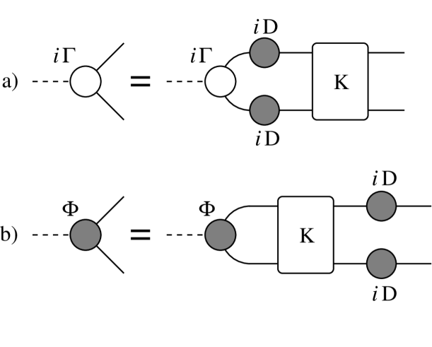
FIG. 1.: Diagrammatic representation of the Bethe-Salpeter equation for (a) the BS vertex ($\Gamma$) and (b) the BS amplitude ($\Phi$). The fully dressed constituent particle propagator is denoted by $D$ and $K$ is the scattering kernel for the constituents.

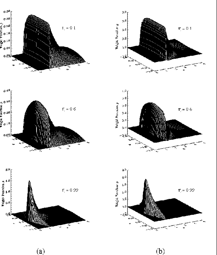
FIG. 2.: Solutions for the bound-state vertex weight function for the $s$-wave ($\ell=0$) and $p$-wave ($\ell=1$) cases are given in (a) and (b) respectively for a variety of values for the fraction of binding $\eta\equiv{\sqrt{P^{2}}}/2m=M/2m$. The exchange particle ($\sigma$) mass is $m_{\sigma}=m/2$ in these solutions. It is convenient to plot the rescaled weight function $\rho(\alpha,z)\equiv\rho_{2}^{[\ell]}(\alpha,z)/\alpha^{2}$ in these figures.

FIG. 3.: The $s$-wave (i.e., $\ell=0$) bound-state spectrum for the ladder kernel, where $\lambda\equiv g^{2}/(4\pi)^{2}$ and $\eta\equiv{\sqrt{P^{2}}}/2m=M/2m$. The exchanged particle ($\sigma$) mass is half the constituent mass, $m_{\sigma}=m/2$, in these results. These results correspond to those in Table I.

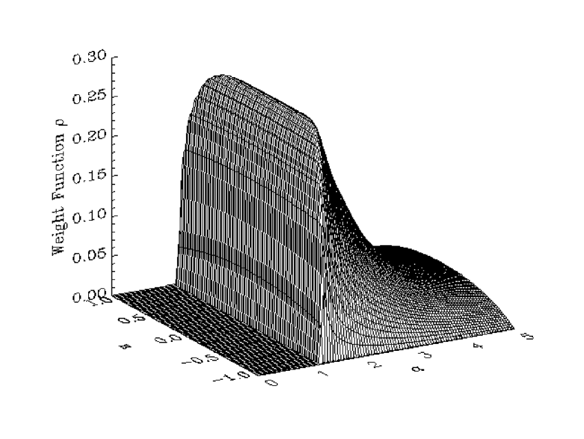
FIG. 4.: Rescaled weight function $\rho(\alpha,z)\equiv\rho_{2}^{[0]}(\alpha,z)/\alpha^{2}$ for the dressed ladder kernel with pole at $m_{\sigma}^{2}=m^{2}$, and a bound-state mass of $\eta\equiv{\sqrt{P^{2}}}/2m=0.1$.

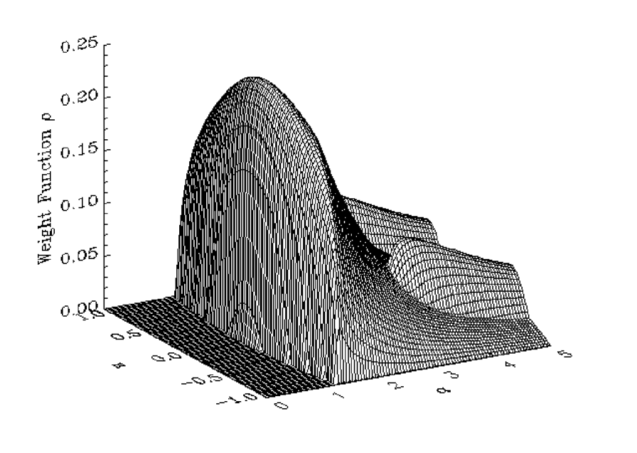
FIG. 5.: Rescaled weight function $\rho(\alpha,z)\equiv\rho_{2}^{[0]}(\alpha,z)/\alpha^{2}$ for a random choice of generalised kernel as described in the text.