Azimuthal Correlation in Lepton-Hadron Scattering
via Charged Weak-Current Processes

Abstract

We consider the azimuthal correlation of the final-state particles in charged weak-current processes. This correlation provides a test of perturbative quantum chromodynamics (QCD). The azimuthal asymmetry is large in the semi-inclusive processes in which we identify a final-state hadron, say, a charged pion compared to that in the inclusive processes in which we do not identify final-state particles and use only the calorimetric information. In semi-inclusive processes the azimuthal asymmetry is more conspicuous when the incident lepton is an antineutrino or a positron than when the incident lepton is a neutrino or an electron. We analyze all the possible charged weak-current processes and study the quantitative aspects of each process. We also compare this result to the $ep$ scattering with a photon exchange.

I Introduction

The QCD-improved parton model has shown a great success in describing high-energy processes such as deep-inelastic leptoproduction. In the parton model we can express the cross section as a convolution of three factors: the parton-lepton hard-scattering cross section, the distribution function describing the partons in the initial state and the fragmentation functions describing the distribution of final-state hadrons from the scattered parton. The hard-scattering cross section at parton level can be calculated at any given order in perturbative QCD. The distribution functions and fragmentation functions themselves cannot be calculated perturbatively but the evolution of these functions can be calculated using perturbation theory.

The azimuthal correlations provide a clean test of perturbative QCD since these correlations occur at higher orders in perturbative QCD. Georgi and Politzer[1] proposed the azimuthal angular dependence of the hadrons in the semi-inclusive processes $\ell+p\rightarrow\ell^{\prime}+h+X$, where $\ell$, $\ell^{\prime}$ are leptons, $h$ is a detected hadron. Cahn[2] included the contribution to the azimuthal angular dependence from the intrinsic transverse momentum of the partons bound inside the proton. Berger[3] considered the final-state interaction producing a pion and found that the azimuthal asymmetry due to this final-state interaction is opposite in sign to that due to the effects studied by Cahn. The azimuthal asymmetries discussed by Cahn and Berger are due to nonperturbative effects. These effects were analyzed at low transverse momentum.[4, 5]

In the kinematic regime attainable at the $ep$ collider at HERA or in the CCFR experiments, we expect that perturbative QCD effects will dominate nonperturbative effects. This is the motivation for considering the azimuthal correlation of final hadrons in $ep$ scattering at HERA and in $\nu p$ $(\overline{\nu}p)$ scattering in CCFR experiments. We consider all the possible charged weak-current processes in the perturbative regime. Méndez et al.[6] considered extensively the azimuthal correlation in leptoproduction. In our paper we analyze the same processes but in different viewpoints and analyses. Especially we direct our focus on the experimental aspects since we can now verify the theoretical results in experiments at HERA or CCFR.

Chay et al.[7] considered the azimuthal asymmetry in $ep$ scattering with a photon exchange. Here we apply a similar analysis used in Ref. [7] to charged weak-current processes in lepton-hadron scattering. The result is striking in the sense that the final-state particles have a strong azimuthal correlation to the incoming lepton. We will systematically analyze the azimuthal asymmetry in this paper. In Sec. II we briefly review the kinematics used in lepton-proton scattering. In Sec. III we define the quantity $\langle\cos\phi\rangle$ as a measure of the azimuthal correlation and calculate it to order $\alpha_{s}$ using perturbative QCD. In Sec. IV we analyze numerically the azimuthal correlation in various processes in which the incoming lepton is an electron, a neutrino, a positron or an antineutrino. We also compare the results from the semi-inclusive processes in which we identify a final-state hadron, say, a charged pion with the results from the inclusive processes in which we use only the calorimetric information, that is, the energy and the momentum of each particle (or each jet). In Sec. V we discuss the behavior of the azimuthal correlation in each process and the conclusion is given in Sec. VI.

II Cross Sections

Here we briefly review the kinematics in lepton-hadron scattering with charged weak currents. Let $k_{1}$ ($k_{2}$) be the initial (final) momentum of the incoming (outgoing) lepton, $P_{1}$ ($P_{2}$) be the target (observed final-state hadron) momentum and $p_{1}$ ($p_{2}$) be the incident (scattered) parton momentum. At high energy, the hadrons will be produced with momenta almost parallel to the virtual $W$-boson direction, $q^{\mu}=k_{1}^{\mu}-k_{2}^{\mu}$. We focus on interactions that produce nonzero transverse momentum ${\bf P}_{2T}$, perpendicular to the spatial component of $q^{\mu}$, which we will denote by ${\bf q}$. We choose the direction of ${\bf q}$ to be the negative $z$ axis. We can write the differential scattering cross section in terms of the following hadronic variables

$$Q^{2} = -q^{2},\ {\bf P}_{T}={\bf P}_{2T},\ \phi,$$ (1)

$$x_{H} = \frac{Q^{2}}{2P_{1}\cdot q},\ y=\frac{P_{1}\cdot q}{P_{1}\cdot k_{1}},\ z_{H}=\frac{P_{1}\cdot P_{2}}{P_{1}\cdot q},$$ (2)

and the partonic variables

$$x=\frac{x_{H}}{\xi}=\frac{Q^{2}}{2p_{1}\cdot q},\ z=\frac{z_{H}}{\xi^{\prime}}=\frac{p_{1}\cdot p_{2}}{p_{1}\cdot q}.$$ (3)

The azimuthal angle $\phi$ of the outgoing hadron is measured with respect to ${\bf k}_{1T}$, whose direction is chosen to be the positive $x$ axis. If we employ jets instead of hadrons, $\phi$ is the azimuthal angle of the jet defined by an appropriate jet algorithm[8] and all the hadronic variables are replaced by the jet variables.

In the parton model, if we consider the inclusive processes $\ell+p\rightarrow\ell^{\prime}+X$, in which $\ell$, $\ell^{\prime}$ are different leptons, the differential cross section is given by

$$\frac{d\sigma}{dx_{H}dydz_{H}d^{2}P_{T}} = \sum_{i}\int dxdzd\xi d^{2}p_{T}\delta(x_{H}-\xi x)\delta(z_{H}-z)$$ (4)

$$\times \delta^{(2)}({\bf P}_{T}-{\bf p}_{T})F_{i}(\xi,Q^{2})\frac{d\hat{\sigma}_{i}}{dxdydzd^{2}p_{T}}$$ (5)

$$= \sum_{i}\int_{x_{H}}^{1}\frac{dx}{x}\int d^{2}p_{T}\delta^{(2)}({\bf P}_{T}-{\bf p}_{T})F_{i}(\frac{x_{H}}{x},Q^{2})\frac{d\hat{\sigma}_{i}}{dxdydzd^{2}p_{T}},$$ (6)

with $d^{2}P_{T}=P_{T}dP_{T}d\phi$. The sum $i$ runs over all types of partons (quarks, antiquarks and gluons) inside the proton and $d\hat{\sigma}_{i}$ is the partonic differential cross section. $F_{i}(x,Q^{2})$ is the parton distribution function of finding the $i$-type parton inside the proton with the momentum fraction $x$. In Eq. (6) we neglect the intrinsic momentum due to the nonperturbative effects and we identify the momentum of the final-state hadron (or a jet) with the momentum of the scattered parton. This approximation is valid if we choose final-state particles with large transverse momenta.

If we consider the semi-inclusive process $\ell+p\rightarrow\ell^{\prime}+h+X$ where $h$ is a detected hadron, say, a charged pion, the differential cross section is given by

$$\frac{d\sigma}{dx_{H}dydz_{H}d^{2}P_{T}} = \sum_{ij}\int dxdzd\xi d\xi^{\prime}d^{2}p_{T}\delta(x_{H}-\xi x)\delta(z_{H}-\xi^{\prime}z)\delta^{(2)}({\bf P}_{T}-\xi^{\prime}{\bf p}_{T})$$ (7)

$$\times F_{i}(\xi,Q^{2})\frac{d\hat{\sigma}_{ij}}{dxdydzd^{2}p_{T}}D_{j}(\xi^{\prime},Q^{2})$$ (8)

$$= \sum_{ij}\int_{x_{H}}^{1}\frac{dx}{x}\int_{z_{H}}^{1}\frac{dz}{z}\int d^{2}p_{T}\delta^{(2)}({\bf P}_{T}-\frac{z_{H}}{z}{\bf p}_{T})$$ (9)

$$\times F_{i}(\frac{x_{H}}{x},Q^{2})\frac{d\hat{\sigma}_{ij}}{dxdydzd^{2}p_{T}}D_{j}(\frac{z_{H}}{z},Q^{2}).$$ (10)

The sum $i$, $j$ runs over all types of partons. The partonic cross setion $d\hat{\sigma}_{ij}$ describes the partonic semi-inclusive process

$$\ell(k_{1})+{\rm parton}\ i(p_{1})\rightarrow\ell^{\prime}(k_{2})+{\rm parton}\ j(p_{2})+X.$$ (11)

Here the exchanged gauge boson is a charged $W$ particle. $F_{i}(x,Q^{2})$ is the $i$-type parton distribution function, $D_{j}(z,Q^{2})$ is the fragmentation function of the $j$-type parton to hadronize into the observed hadron $h$ with the momentum fraction $z$. These two types of functions depend on factorization scales and for simplicity we put the scale to be $Q$, a typical scale in lepton-hadron scattering.

In order to obtain hadronic cross sections, we have to calculate partonic cross sections using perturbative QCD. At zeroth order in $\alpha_{s}$, the parton cross section for the scattering $\nu+q\rightarrow e+q^{\prime}$ is given by

$$\frac{d\hat{\sigma}_{q}}{dxdydzd^{2}p_{T}}=\frac{G_{F}^{2}m_{W}^{4}|V_{q^{\prime}q}|^{2}}{\pi}\frac{Q^{2}}{(Q^{2}+m_{W}^{2})^{2}}\frac{1}{y}\delta(1-x)\delta(1-z)\delta^{2}({\bf p}_{T}),$$ (12)

where $V_{q^{\prime}q}$ is the relevant Cabibbo-Kobayashi-Maskawa (CKM) matrix element for the process $W^{+}+q\rightarrow q^{\prime}$. $G_{F}$ is the Fermi constant and $m_{W}$ is the mass of the $W$ gauge boson. For the scattering of an antiquark with a neutrino, $\nu+\overline{q}\rightarrow e+\overline{q}^{\prime}$, the parton cross section is given by

$$\frac{d\hat{\sigma}_{\overline{q}}}{dxdydzd^{2}p_{T}}=\frac{G_{F}^{2}m_{W}^{4}|V_{qq^{\prime}}|^{2}}{\pi}\frac{Q^{2}}{(Q^{2}+m_{W}^{2})^{2}}\frac{(1-y)^{2}}{y}\delta(1-x)\delta(1-z)\delta^{2}({\bf p}_{T}).$$ (13)

The only difference between these cross sections in Eqs. (12) and (13) is the appearance of the factor $(1-y)^{2}$. This is due to the helicity conservation. In short, when particles with the opposite handedness scatter, we have the factor of $(1-y)^{2}$ in front, while it is independent of $y$ when particles with the same handedness scatter. The cross sections for other processes like $e+q\ (\overline{q})\rightarrow\nu+q^{\prime}\ (\overline{q^{\prime}})$, $\overline{\nu}+q\ (\overline{q})\rightarrow e^{+}+q^{\prime}\ (\overline{q}^{\prime})$ and $e^{+}+q\ (\overline{q})\rightarrow\nu+q^{\prime}\ (\overline{q^{\prime}})$ can be obtained using crossing symmetries. However since the transverse momentum is zero at this order, there is no azimuthal correlation at the Born level.

FIG. 1.: Feynman diagrams for charged weak-current processes at order $\alpha_{s}$.

To first order in $\alpha_{s}$, the parton scattering processes develop nonzero $p_{T}$ and nontrivial dependence on the azimuthal angle $\phi$. The relevant processes are

$$q(p_{1})+W^{\pm*}(q) \rightarrow q^{\prime}(p_{2})+g(p_{3}),$$ (14)

$$q(p_{1})+W^{\pm*}(q) \rightarrow q^{\prime}(p_{3})+g(p_{2}),$$ (15)

$$\overline{q}(p_{1})+W^{\pm*}(q) \rightarrow \overline{q}^{\prime}(p_{2})+g(p_{3}),$$ (16)

$$\overline{q}(p_{1})+W^{\pm*}(q) \rightarrow \overline{q}^{\prime}(p_{3})+g(p_{2}),$$ (17)

$$g(p_{1})+W^{\pm*}(q) \rightarrow q(p_{2})+\overline{q}^{\prime}(p_{3}),$$ (18)

$$g(p_{1})+W^{\pm*}(q) \rightarrow q(p_{3})+\overline{q}^{\prime}(p_{2}),$$ (19)

where $g$ is a gluon, $W^{\pm*}$ is the virtual $W$ boson and $q$, $q^{\prime}$ are quarks. The Feynman diagrams for these processes are shown in Fig. 1. Fig. 1(a) corresponds to Eq. (14) [Eq. (16)] with a quark line (an antiquark line) and similarly Fig. 1(b) corresponds to Eq. (15) and Eq. (17). Fig. 1(c) and Fig. 1(d) correspond to Eq. (18) and Eq. (19) respectively.

Using the Sudakov parametrization we can express $p_{2}$ in terms of $x$, $y$ and $z$ as

$$p_{2}^{\mu}=\Bigl{[}(1-x)(1-z)+xz\Bigr{]}p_{1}^{\mu}+zq^{\mu}+\tilde{p}_{T}^{\mu},$$ (20)

where $\tilde{p}_{T}=(0,{\bf p}_{T},0)$ is the transverse momentum with $p_{1}\cdot\tilde{p}_{T}=q\cdot\tilde{p}_{T}=0$. For massless partons we have

$$p_{T}^{2}=|{\bf p}_{2T}|^{2}=\frac{z}{x}(1-x)(1-z)Q^{2}.$$ (21)

Similarly we can write

$$k_{1}^{\mu}=\frac{x}{y}(2-y)p_{1}^{\mu}+\frac{1}{y}q^{\mu}+\tilde{k}_{T}^{\mu},$$ (22)

with $k_{T}^{2}=(1-y)Q^{2}/y^{2}$, where $\tilde{k}_{T}$ is defined in the same way as $\tilde{p}_{T}$. Therefore we have

$$k_{1}\cdot p_{2}=\frac{Q^{2}}{2xy}\Bigl{[}(1-x)(1-z)+xz(1-y)\Bigr{]}-{\bf k}_{T}\cdot{\bf p}_{T},$$ (23)

and

$$k_{2}\cdot p_{2}=\frac{Q^{2}}{2xy}\Bigl{[}(1-x)(1-y)(1-z)+xz\Bigr{]}-{\bf k}_{T}\cdot{\bf p}_{T}.$$ (24)

The semi-inclusive parton scattering cross section for charged weak-current is given by

$$\frac{d\hat{\sigma}_{ij}}{dxdydzd^{2}p_{T}}=\frac{\alpha_{s}G_{F}^{2}m_{W}^{4}|V_{q^{\prime}q}|^{2}}{2\pi^{3}}\frac{yQ^{2}}{(Q^{2}+m_{W}^{2})^{2}}L_{\mu\nu}M_{ij}^{\mu\nu}\delta\Bigl{(}p_{T}^{2}-\frac{z}{x}(1-x)(1-z)Q^{2}\Bigr{)},$$ (25)

where $L_{\mu\nu}$ is the average squared of the leptonic charged current and $M_{ij}^{\mu\nu}$ is the partonic tensor for the incoming parton $i$ and the outgoing parton $j$. $V_{q^{\prime}q}$ are the CKM matrix elements. The products $L_{\mu\nu}M_{ij}^{\mu\nu}$ for the processes in Eqs. (14), (15), (16), (17), (18) and (19), i.e., $ij=qq$, $qg$, $\overline{q}\overline{q}$, $\overline{q}g$, $gq$ and $g\overline{q}$ depend on the types of incoming leptons. For the process $\nu+{\rm parton}\ i\rightarrow e+{\rm parton}\ j+X$, they are written as

$$L_{\mu\nu}M_{qq}^{\mu\nu} = \frac{4}{3}\frac{(k_{1}\cdot p_{1})^{2}+(k_{2}\cdot p_{2})^{2}}{p_{1}\cdot p_{3}\ p_{2}\cdot p_{3}},$$ (26)

$$L_{\mu\nu}M_{qg}^{\mu\nu} = \frac{4}{3}\frac{(k_{1}\cdot p_{1})^{2}+(k_{2}\cdot p_{3})^{2}}{p_{1}\cdot p_{2}\ p_{2}\cdot p_{3}},$$ (27)

$$L_{\mu\nu}M_{\overline{q}\overline{q}}^{\mu\nu} = \frac{4}{3}\frac{(k_{1}\cdot p_{2})^{2}+(k_{2}\cdot p_{1})^{2}}{p_{1}\cdot p_{3}\ p_{2}\cdot p_{3}},$$ (28)

$$L_{\mu\nu}M_{\overline{q}g}^{\mu\nu} = \frac{4}{3}\frac{(k_{1}\cdot p_{3})^{2}+(k_{2}\cdot p_{1})^{2}}{p_{1}\cdot p_{2}\ p_{2}\cdot p_{3}},$$ (29)

$$L_{\mu\nu}M_{gq}^{\mu\nu} = \frac{1}{2}\frac{(k_{1}\cdot p_{3})^{2}+(k_{2}\cdot p_{2})^{2}}{p_{1}\cdot p_{2}\ p_{1}\cdot p_{3}},$$ (30)

$$L_{\mu\nu}M_{g\overline{q}}^{\mu\nu} = \frac{1}{2}\frac{(k_{1}\cdot p_{2})^{2}+(k_{2}\cdot p_{3})^{2}}{p_{1}\cdot p_{2}\ p_{1}\cdot p_{3}}.$$ (31)

Eqs. (26) and (27) correspond to the Feynman diagrams with quarks in Fig. 1(a) and 1(b) respectively with quarks, Eqs. (28) and (29) correspond to the same diagrams with antiquarks. Eqs. (30) and (31) correspond to Fig. 1(c) and 1(d) respectively. Note that Eqs. (27), (29) and (31) are obtained from Eqs. (26), (28) and (30) respectively by switching $p_{2}$ and $p_{3}$. And Eq. (28) is obtained from Eq. (26) by switching $p_{1}$ and $p_{2}$. For the process $e+{\rm parton}\ i\rightarrow\nu+{\rm parton}\ j+X$, the matrix elements squared are the same as Eqs. (26)–(31) except an extra factor of 1/2 taking into account the spin average of the incoming electron.

With the Eqs. (26)–(31), we can also obtain $L_{\mu\nu}M_{ij}^{\mu\nu}$ for other charged weak-current processes. For example, for the processes $\overline{\nu}+{\rm parton}\ i\rightarrow e^{+}+{\rm parton}\ j+X$, $L_{\mu\nu}M_{ij}^{\mu\nu}$ are obtained by switching $k_{1}$ and $k_{2}$ in Eqs. (26)–(31). They are written as

$$L_{\mu\nu}M_{qq}^{\mu\nu} = \frac{4}{3}\frac{(k_{2}\cdot p_{1})^{2}+(k_{1}\cdot p_{2})^{2}}{p_{1}\cdot p_{3}\ p_{2}\cdot p_{3}},$$ (32)

$$L_{\mu\nu}M_{qg}^{\mu\nu} = \frac{4}{3}\frac{(k_{2}\cdot p_{1})^{2}+(k_{1}\cdot p_{3})^{2}}{p_{1}\cdot p_{2}\ p_{2}\cdot p_{3}},$$ (33)

$$L_{\mu\nu}M_{\overline{q}\overline{q}}^{\mu\nu} = \frac{4}{3}\frac{(k_{2}\cdot p_{2})^{2}+(k_{1}\cdot p_{1})^{2}}{p_{1}\cdot p_{3}\ p_{2}\cdot p_{3}},$$ (34)

$$L_{\mu\nu}M_{\overline{q}g}^{\mu\nu} = \frac{4}{3}\frac{(k_{2}\cdot p_{3})^{2}+(k_{1}\cdot p_{1})^{2}}{p_{1}\cdot p_{2}\ p_{2}\cdot p_{3}},$$ (35)

$$L_{\mu\nu}M_{gq}^{\mu\nu} = \frac{1}{2}\frac{(k_{2}\cdot p_{3})^{2}+(k_{1}\cdot p_{2})^{2}}{p_{1}\cdot p_{2}\ p_{1}\cdot p_{3}},$$ (36)

$$L_{\mu\nu}M_{g\overline{q}}^{\mu\nu} = \frac{1}{2}\frac{(k_{2}\cdot p_{2})^{2}+(k_{1}\cdot p_{3})^{2}}{p_{1}\cdot p_{2}\ p_{1}\cdot p_{3}}.$$ (37)

By the same argument $L_{\mu\nu}M_{ij}^{\mu\nu}$ for the process $e^{+}+{\rm parton}\ i\rightarrow\overline{\nu}+{\rm parton}\ j+X$ are the same except a factor of 1/2.

III Azimuthal Asymmetry

The azimuthal asymmetry can be characterized by the average value of $\cos\phi$, which measures the front-back asymmetry of ${\bf P}_{2T}$ along the ${\bf k}_{1T}$ direction. It is defined by

$$\langle\cos\phi\rangle=\frac{\displaystyle\int\Bigl{(}d\sigma^{(0)}+d\sigma^{(1)}\Bigr{)}\cos\phi}{\displaystyle\int\Bigl{(}d\sigma^{(0)}+d\sigma^{(1)}\Bigr{)}},$$ (38)

where $d\sigma^{(0)}$ ($d\sigma^{(1)}$) is the lowest-order (first-order in $\alpha_{s}$) hadronic scattering cross section defined in Eqs. (6) or (10) and the integration over $P_{T}$, $\phi$, $x_{H}$, $y$ and $z_{H}$ is implied. When we impose a nonzero transverse momentum cutoff, Eq. (38) receives contributions only from $d\sigma^{(1)}$ both in the numerator and in the denominator. Note that the zeroth-order cross section is proportional to $\delta({\bf P}_{T})$. Therefore with the nonzero transverse momentum cutoff at order $\alpha_{s}$ in perturbation theory, the quantity $\langle\cos\phi\rangle$ is independent of $\alpha_{s}$.

In fact the azimuthal asymmetry can occur at the Born level if we include the intrinsic transverse momentum due to the confinement of partons inside a proton and the fragementation process for partons into hadrons[2, 3, 7]. However the size of the intrinsic transverse momentum due to nonperturbative effects is of the order of a few hundred MeV. Therefore if we make the transverse momentum cutoff $p_{c}$ large enough ($\geq 2$ GeV) and choose hadrons with the transverse momenta larger than $p_{c}$, we expect that the contributions from the intrinsic transverse momentum from the Born-level processes are negligible compared to those from $\sigma^{(1)}$. In other words the intrinsic transverse momenta of the partons simply cannot produce hadrons with transverse momenta larger than $p_{c}$ and the effects from intrinsic transverse momenta are suppressed. Therefore, for $p_{c}$ larger than 2 GeV, $\langle\cos\phi\rangle$ is given by, to a good approximation,

$$\langle\cos\phi\rangle\simeq\frac{\displaystyle\int d\sigma^{(1)}\cos\phi}{\displaystyle\int d\sigma^{(1)}}.$$ (39)

In the following analysis we consider $\langle\cos\phi\rangle$ as a function of the transverse momentum cutoff $p_{c}$.

We first consider the azimuthal asymmetry in the inclusive process $\nu+p\rightarrow e+X$, where $X$ denotes any hadron. The numerator in Eq. (39) can be written as

$$\int d\sigma^{(1)}\cos\phi = \int d^{2}P_{T}\cos\phi\frac{d\sigma}{dx_{H}dydz_{H}d^{2}P_{T}}$$ (40)

$$= \frac{8\alpha_{s}G_{F}^{2}m_{W}^{4}}{3\pi^{2}}\frac{Q^{2}}{(Q^{2}+m_{W}^{2})^{2}}\frac{1}{y}$$ (41)

$$\times \int_{x_{H}}^{1}\frac{dx}{x}(A_{\nu}+B_{\nu}+C_{\nu}+D_{\nu}+E_{\nu}+F_{\nu}),$$ (42)

where

$$A_{\nu} = -\sqrt{\frac{(1-y)xz}{(1-x)(1-z)}}\Bigl{[}(1-y)(1-x)(1-z)+xz\Bigr{]}$$ (43)

$$\times \Bigl{(}|V_{ud}|^{2}F_{d}(\frac{x_{H}}{x},Q^{2})+|V_{cs}|^{2}F_{s}(\frac{x_{H}}{x},Q^{2})\Bigr{)},$$ (44)

$$B_{\nu} = \sqrt{\frac{(1-y)x(1-z)}{(1-x)z}}\Bigl{[}(1-y)(1-x)z+x(1-z)\Bigr{]}$$ (45)

$$\times \Bigl{(}|V_{ud}|^{2}F_{d}(\frac{x_{H}}{x},Q^{2})+|V_{cs}|^{2}F_{s}(\frac{x_{H}}{x},Q^{2})\Bigr{)},$$ (46)

$$C_{\nu} = -\sqrt{\frac{(1-y)xz}{(1-x)(1-z)}}\Bigl{[}(1-x)(1-z)+(1-y)xz\Bigr{]}$$ (47)

$$\times \Bigl{(}|V_{ud}|^{2}F_{\overline{u}}(\frac{x_{H}}{x},Q^{2})+|V_{cs}|^{2}F_{\overline{c}}(\frac{x_{H}}{x},Q^{2})\Bigr{)},$$ (48)

$$D_{\nu} = \sqrt{\frac{(1-y)x(1-z)}{(1-x)z}}\Bigl{[}(1-x)z+(1-y)x(1-z)\Bigr{]}$$ (49)

$$\times \Bigl{(}|V_{ud}|^{2}F_{\overline{u}}(\frac{x_{H}}{x},Q^{2})+|V_{cs}|^{2}F_{\overline{c}}(\frac{x_{H}}{x},Q^{2})\Bigr{)},$$ (50)

$$E_{\nu} = \frac{3}{8}(1-2x)\sqrt{\frac{(1-y)x(1-x)}{z(1-z)}}\Bigl{[}z-(1-y)(1-z)\Bigr{]}$$ (51)

$$\times \Bigl{(}|V_{ud}|^{2}+|V_{cs}|^{2}\Bigr{)}F_{g}(\frac{x_{H}}{x},Q^{2})\Bigr{)},$$ (52)

$$F_{\nu} = -\frac{3}{8}(1-2x)\sqrt{\frac{(1-y)x(1-x)}{z(1-z)}}\Bigl{[}1-z-(1-y)z\Bigr{]}$$ (53)

$$\times \Bigl{(}|V_{ud}|^{2}+|V_{cs}|^{2}\Bigr{)}F_{g}(\frac{x_{H}}{x},Q^{2})\Bigr{)}.$$ (54)

The denominator can be written as

$$\int d\sigma^{(1)} = \int d^{2}P_{T}\frac{d\sigma}{dx_{H}dydz_{H}d^{2}P_{T}}$$ (55)

$$= \frac{4\alpha_{s}G_{F}^{2}m_{W}^{4}}{3\pi^{2}}\frac{Q^{2}}{(Q^{2}+m_{W}^{2})^{2}}\frac{1}{y}$$ (56)

$$\times \int_{x_{H}}^{1}\frac{dx}{x}(A^{\prime}_{\nu}+B^{\prime}_{\nu}+C^{\prime}_{\nu}+D^{\prime}_{\nu}+E^{\prime}_{\nu}+F^{\prime}_{\nu}),$$ (57)

where

$$A_{\nu}^{\prime} = \Bigl{[}\frac{1+x^{2}z^{2}}{(1-x)(1-z)}+4(1-y)xz+(1-y)^{2}(1-x)(1-z)\Bigr{]}$$ (58)

$$\times \Bigl{(}|V_{ud}|^{2}F_{d}(\frac{x_{H}}{x},Q^{2})+|V_{cs}|^{2}F_{s}(\frac{x_{H}}{x},Q^{2})\Bigr{)},$$ (59)

$$B_{\nu}^{\prime} = \Bigl{[}\frac{1+x^{2}(1-z)^{2}}{(1-x)z}+4(1-y)x(1-z)+(1-y)^{2}(1-x)z\Bigr{]}$$ (60)

$$\times \Bigl{(}|V_{ud}|^{2}F_{d}(\frac{x_{H}}{x},Q^{2})+|V_{cs}|^{2}F_{s}(\frac{x_{H}}{x},Q^{2})\Bigr{)},$$ (61)

$$C_{\nu}^{\prime} = \Bigl{[}(1-y)^{2}\frac{1+x^{2}z^{2}}{(1-x)(1-z)}+4(1-y)xz+(1-x)(1-z)\Bigr{]}$$ (62)

$$\times \Bigl{(}|V_{ud}|^{2}F_{\overline{u}}(\frac{x_{H}}{x},Q^{2})+|V_{cs}|^{2}F_{\overline{c}}(\frac{x_{H}}{x},Q^{2})\Bigr{)},$$ (63)

$$D_{\nu}^{\prime} = \Bigl{[}(1-y)^{2}\frac{1+x^{2}(1-z)^{2}}{(1-x)z}+4(1-y)x(1-z)+(1-x)z\Bigr{]}$$ (64)

$$\times \Bigl{(}|V_{ud}|^{2}F_{\overline{u}}(\frac{x_{H}}{x},Q^{2})+|V_{cs}|^{2}F_{\overline{c}}(\frac{x_{H}}{x},Q^{2})\Bigr{)},$$ (65)

$$E_{\nu}^{\prime} = \frac{3}{8}\Bigl{[}\Bigl{(}z^{2}+(1-y)^{2}(1-z)^{2}\Bigr{)}\frac{x^{2}+(1-x)^{2}}{z(1-z)}+8(1-y)x(1-x)$$ (66)

$$\times \Bigl{(}|V_{ud}|^{2}+|V_{cs}|^{2}\Bigr{)}F_{g}(\frac{x_{H}}{x},Q^{2}),$$ (67)

$$F_{\nu}^{\prime} = \frac{3}{8}\Bigl{[}\Bigl{(}(1-z)^{2}+(1-y)^{2}z^{2}\Bigr{)}\frac{x^{2}+(1-x)^{2}}{z(1-z)}+8(1-y)x(1-x)\Bigr{]}$$ (68)

$$\times \Bigl{(}|V_{ud}|^{2}+|V_{cs}|^{2}\Bigr{)}F_{g}(\frac{x_{H}}{x},Q^{2}).$$ (69)

The above six terms in Eqs. (54) and (69) are obtained from the matrix elements in Eqs. (26)–(31) respectively. For the inclusive process $e+p\rightarrow\nu+X$, the corresponding quantities are the same except that the quark flavors are switched, $u\leftrightarrow d$ and $c\leftrightarrow s$ in the parton distributions functions. There should also be a factor 1/2 from the incoming electron spin average. However it appears both in the numerator and in the denominator, hence cancels out.

Now consider the inclusive process $\overline{\nu}+p\rightarrow e^{+}+X$. The numerator and the denominator in defining $\langle\cos\phi\rangle$ as in Eqs. (42) and (57) are given by

$$A_{\overline{\nu}} = -\sqrt{\frac{(1-y)xz}{(1-x)(1-z)}}\Bigl{[}(1-x)(1-z)+(1-y)xz\Bigr{]}$$ (70)

$$\times \Bigl{(}|V_{ud}|^{2}F_{u}(\frac{x_{H}}{x},Q^{2})+|V_{cs}|^{2}F_{c}(\frac{x_{H}}{x},Q^{2})\Bigr{)},$$ (71)

$$B_{\overline{\nu}} = \sqrt{\frac{(1-y)x(1-z)}{(1-x)z}}\Bigl{[}(1-x)z+(1-y)x(1-z)\Bigr{]}$$ (72)

$$\times \Bigl{(}|V_{ud}|^{2}F_{u}(\frac{x_{H}}{x},Q^{2})+|V_{cs}|^{2}F_{c}(\frac{x_{H}}{x},Q^{2})\Bigr{)},$$ (73)

$$C_{\overline{\nu}} = -\sqrt{\frac{(1-y)xz}{(1-x)(1-z)}}\Bigl{[}(1-y)(1-x)(1-z)+xz\Bigr{]}$$ (74)

$$\times \Bigl{(}|V_{ud}|^{2}F_{\overline{d}}(\frac{x_{H}}{x},Q^{2})+|V_{cs}|^{2}F_{\overline{d}}(\frac{x_{H}}{x},Q^{2})\Bigr{)},$$ (75)

$$D_{\overline{\nu}} = \sqrt{\frac{(1-y)x(1-z)}{(1-x)z}}\Bigl{[}(1-y)(1-x)z+x(1-z)\Bigr{]}$$ (76)

$$\times \Bigl{(}|V_{ud}|^{2}F_{\overline{d}}(\frac{x_{H}}{x},Q^{2})+|V_{cs}|^{2}F_{\overline{s}}(\frac{x_{H}}{x},Q^{2})\Bigr{)},$$ (77)

$$E_{\overline{\nu}} = -\frac{3}{8}(1-2x)\sqrt{\frac{x(1-x)(1-y)}{z(1-z)}}\Bigl{[}1-z-z(1-y)\Bigr{]}$$ (78)

$$\times \Bigl{(}|V_{ud}|^{2}+|V_{cs}|^{2}\Bigr{)}F_{g}(\frac{x_{H}}{x},Q^{2}),$$ (79)

$$F_{\overline{\nu}} = \frac{3}{8}(1-2x)\sqrt{\frac{(1-y)x(1-x)}{z(1-z)}}\Bigl{[}z-(1-y)(1-z)\Bigr{]}$$ (80)

$$\times \Bigl{(}|V_{ud}|^{2}+|V_{cs}|^{2}\Bigr{)}F_{g}(\frac{x_{H}}{x},Q^{2}),$$ (81)

and

$$A_{\overline{\nu}}^{\prime} = \Bigl{[}(1-y)^{2}\frac{1+x^{2}z^{2}}{(1-x)(1-z)}+4(1-y)xz+(1-x)(1-z)\Bigr{]}$$ (82)

$$\times \Bigl{(}|V_{ud}|^{2}F_{u}(\frac{x_{H}}{x},Q^{2})+|V_{cs}|^{2}F_{c}(\frac{x_{H}}{x},Q^{2})\Bigr{)},$$ (83)

$$B_{\overline{\nu}}^{\prime} = \Bigl{[}(1-y)^{2}\frac{1+x^{2}(1-z)^{2}}{(1-x)z}+4(1-y)x(1-z)+(1-x)z\Bigr{]}$$ (84)

$$\times \Bigl{(}|V_{ud}|^{2}F_{u}(\frac{x_{H}}{x},Q^{2})+|V_{cs}|^{2}F_{c}(\frac{x_{H}}{x},Q^{2})\Bigr{)},$$ (85)

$$C_{\overline{\nu}}^{\prime} = \Bigl{[}\frac{1+x^{2}z^{2}}{(1-x)(1-z)}+4(1-y)xz+(1-y)^{2}(1-x)(1-z)\Bigr{]}$$ (86)

$$\times \Bigl{(}|V_{ud}|^{2}F_{\overline{d}}(\frac{x_{H}}{x},Q^{2})+|V_{cs}|^{2}F_{\overline{s}}(\frac{x_{H}}{x},Q^{2})\Bigr{)},$$ (87)

$$D_{\overline{\nu}}^{\prime} = \Bigl{[}\frac{1+x^{2}(1-z)^{2}}{(1-x)z}+4(1-y)x(1-z)+(1-y)^{2}(1-x)z\Bigr{]}$$ (88)

$$\times \Bigl{(}|V_{ud}|^{2}F_{\overline{d}}(\frac{x_{H}}{x},Q^{2})+|V_{cs}|^{2}F_{\overline{s}}(\frac{x_{H}}{x},Q^{2})\Bigr{)},$$ (89)

$$E_{\overline{\nu}}^{\prime} = \frac{3}{8}\Bigl{[}\Bigl{(}(1-z)^{2}+(1-y)^{2}z^{2}\Bigr{)}\frac{x^{2}+(1-x)^{2}}{z(1-z)}+8(1-y)x(1-x)\Bigr{]}$$ (90)

$$\times \Bigl{(}|V_{ud}|^{2}+|V_{cs}|^{2}\Bigr{)}F_{g}(\frac{x_{H}}{x},Q^{2}),$$ (91)

$$F_{\overline{\nu}}^{\prime} = \frac{3}{8}\Bigl{[}\Bigl{(}z^{2}+(1-y)^{2}(1-z)^{2}\Bigr{)}\frac{x^{2}+(1-x)^{2}}{z(1-z)}+8(1-y)x(1-x)\Bigr{]}$$ (92)

$$\times \Bigl{(}|V_{ud}|^{2}+|V_{cs}|^{2}\Bigr{)}F_{g}(\frac{x_{H}}{x},Q^{2}).$$ (93)

For the process $e^{+}+p\rightarrow\overline{\nu}+X$, the corresponding quantities are the same as in Eqs. (81) and (93) except the switch of the quark flavors $u\leftrightarrow d$ and $c\leftrightarrow s$ in the parton distribution functions.

We can express $\langle\cos\phi\rangle$ using Eq. (10) in the semi-inclusive processes in which we identify a final-state charged pion. For the process $\nu+p\rightarrow e+\pi+X$, the numerator can be written as

$$\int d\sigma^{(1)}\cos\phi = \frac{8\alpha_{s}G_{F}^{2}m_{W}^{4}}{3\pi^{2}}\frac{Q^{2}}{(Q^{2}+m_{W}^{2})^{2}}\frac{1}{y}$$ (94)

$$\times \int_{x_{H}}^{1}\frac{dx}{x}\int_{z_{H}}^{1}\frac{dz}{z}(a_{\nu}+b_{\nu}+c_{\nu}+d_{\nu}+e_{\nu}+f_{\nu}),$$ (95)

and the denominator can be written as

$$\int d\sigma^{(1)} = \frac{4\alpha_{s}G_{F}^{2}m_{W}^{4}}{3\pi^{2}}\frac{Q^{2}}{(Q^{2}+m_{W}^{2})^{2}}\frac{1}{y}$$ (96)

$$\times \int_{x_{H}}^{1}\frac{dx}{x}\int_{z_{H}}^{1}\frac{dz}{z}(a^{\prime}_{\nu}+b^{\prime}_{\nu}+c^{\prime}_{\nu}+d^{\prime}_{\nu}+e^{\prime}_{\nu}+f^{\prime}_{\nu}).$$ (97)

The quantities introduced in Eqs. (95) and (97) are given as follows:

$$a_{\nu} = -\sqrt{\frac{(1-y)xz}{(1-x)(1-z)}}\Bigl{[}(1-y)(1-x)(1-z)+xz\Bigr{]}$$ (98)

$$\times \Bigl{(}|V_{ud}|^{2}F_{d}(\frac{x_{H}}{x},Q^{2})D_{u}^{\pi}(\frac{z_{H}}{z},Q^{2})+|V_{cs}|^{2}F_{s}(\frac{x_{H}}{x},Q^{2})D_{c}^{\pi}(\frac{z_{H}}{z},Q^{2})\Bigr{)},$$ (99)

$$b_{\nu} = \sqrt{\frac{(1-y)x(1-z)}{(1-x)z}}\Bigl{[}(1-y)(1-x)z+x(1-z)\Bigr{]}$$ (100)

$$\times \Bigl{(}|V_{ud}|^{2}F_{d}(\frac{x_{H}}{x},Q^{2})+|V_{cs}|^{2}F_{s}(\frac{x_{H}}{x},Q^{2})\Bigr{)}D_{g}^{\pi}(\frac{z_{H}}{z},Q^{2}),$$ (101)

$$c_{\nu} = -\sqrt{\frac{(1-y)xz}{(1-x)(1-z)}}\Bigl{[}(1-x)(1-z)+(1-y)xz\Bigr{]}$$ (102)

$$\times \Bigl{(}|V_{ud}|^{2}F_{\overline{u}}(\frac{x_{H}}{x},Q^{2})D_{\overline{d}}^{\pi}(\frac{z_{H}}{z},Q^{2})+|V_{cs}|^{2}F_{\overline{c}}(\frac{x_{H}}{x},Q^{2})D_{\overline{s}}^{\pi}(\frac{z_{H}}{z},Q^{2})\Bigr{)},$$ (103)

$$d_{\nu} = \sqrt{\frac{(1-y)x(1-z)}{(1-x)z}}\Bigl{[}(1-x)z+(1-y)x(1-z)\Bigr{]}$$ (104)

$$\times \Bigl{(}|V_{ud}|^{2}F_{\overline{u}}(\frac{x_{H}}{x},Q^{2})+|V_{cs}|^{2}F_{\overline{c}}(\frac{x_{H}}{x},Q^{2})\Bigr{)}D_{g}^{\pi}(\frac{z_{H}}{z},Q^{2}),$$ (105)

$$e_{\nu} = \frac{3}{8}(1-2x)\sqrt{\frac{(1-y)x(1-x)}{z(1-z)}}\Bigl{[}z-(1-y)(1-z)\Bigr{]}$$ (106)

$$\times \Bigl{(}|V_{ud}|^{2}D_{u}^{\pi}(\frac{z_{H}}{z},Q^{2})+|V_{cs}|^{2}D_{c}^{\pi}(\frac{z_{H}}{z},Q^{2})\Bigr{)}F_{g}(\frac{x_{H}}{x},Q^{2}),$$ (107)

$$f_{\nu} = -\frac{3}{8}(1-2x)\sqrt{\frac{(1-y)x(1-x)}{z(1-z)}}\Bigl{[}1-z-(1-y)z\Bigr{]}$$ (108)

$$\times \Bigl{(}|V_{ud}|^{2}D_{\overline{d}}^{\pi}(\frac{z_{H}}{z},Q^{2})+|V_{cs}|^{2}D_{\overline{s}}^{\pi}(\frac{z_{H}}{z},Q^{2})\Bigr{)}F_{g}(\frac{x_{H}}{x},Q^{2}),$$ (109)

where $D_{i}^{\pi}(z_{H}/z,Q^{2})$ is the fragmentation function for the $i$-type parton to fragment into a charged pion.

The quantities in the denominator are given by

$$a_{\nu}^{\prime} = \Bigl{[}\frac{1+x^{2}z^{2}}{(1-x)(1-z)}+4(1-y)xz+(1-y)^{2}(1-x)(1-z)\Bigr{]}$$ (110)

$$\times \Bigl{(}|V_{ud}|^{2}F_{d}(\frac{x_{H}}{x},Q^{2})D_{u}^{\pi}(\frac{z_{H}}{z},Q^{2})+|V_{cs}|^{2}F_{s}(\frac{x_{H}}{x},Q^{2})D_{c}^{\pi}(\frac{z_{H}}{z},Q^{2})\Bigr{)},$$ (111)

$$b_{\nu}^{\prime} = \Bigl{[}\frac{1+x^{2}(1-z)^{2}}{(1-x)z}+4(1-y)x(1-z)+(1-y)^{2}(1-x)z\Bigr{]}$$ (112)

$$\times \Bigl{(}|V_{ud}|^{2}F_{d}(\frac{x_{H}}{x},Q^{2})+|V_{cs}|^{2}F_{s}(\frac{x_{H}}{x},Q^{2})\Bigr{)}D_{g}^{\pi}(\frac{z_{H}}{z},Q^{2}),$$ (113)

$$c_{\nu}^{\prime} = \Bigl{[}(1-y)^{2}\frac{1+x^{2}z^{2}}{(1-x)(1-z)}+4(1-y)xz+(1-x)(1-z)\Bigr{]}$$ (114)

$$\times \Bigl{(}|V_{ud}|^{2}F_{\overline{u}}(\frac{x_{H}}{x},Q^{2})D_{\overline{d}}^{\pi}(\frac{z_{H}}{z},Q^{2})+|V_{cs}|^{2}F_{\overline{c}}(\frac{x_{H}}{x},Q^{2})D_{\overline{s}}^{\pi}(\frac{z_{H}}{z},Q^{2})\Bigr{)},$$ (115)

$$d_{\nu}^{\prime} = \Bigl{[}(1-y)^{2}\frac{1+x^{2}(1-z)^{2}}{(1-x)z}+4(1-y)x(1-z)+(1-x)z\Bigr{]}$$ (116)

$$\times \Bigl{(}|V_{ud}|^{2}F_{\overline{u}}(\frac{x_{H}}{x},Q^{2})+|V_{cs}|^{2}F_{\overline{c}}(\frac{x_{H}}{x},Q^{2})\Bigr{)}D_{g}^{\pi}(\frac{z_{H}}{z},Q^{2}),$$ (117)

$$e_{\nu}^{\prime} = \frac{3}{8}\Bigl{[}\Bigl{(}z^{2}+(1-y)^{2}(1-z)^{2}\Bigr{)}\frac{x^{2}+(1-x)^{2}}{z(1-z)}+8(1-y)x(1-x)\Bigr{]}$$ (118)

$$\times \Bigl{(}|V_{ud}|^{2}D_{u}^{\pi}(\frac{z_{H}}{z},Q^{2})+|V_{cs}|^{2}D_{c}^{\pi}(\frac{z_{H}}{z},Q^{2})\Bigr{)}F_{g}(\frac{x_{H}}{x},Q^{2}),$$ (119)

$$f_{\nu}^{\prime} = \frac{3}{8}\Bigl{[}\Bigl{(}(1-z)^{2}+(1-y)^{2}z^{2}\Bigr{)}\frac{x^{2}+(1-x)^{2}}{z(1-z)}+8(1-y)x(1-x)\Bigr{]}$$ (120)

$$\times \Bigl{(}|V_{ud}|^{2}D_{\overline{d}}^{\pi}(\frac{z_{H}}{z},Q^{2})+|V_{cs}|^{2}D_{\overline{s}}^{\pi}(\frac{z_{H}}{z},Q^{2})\Bigr{)}F_{g}(\frac{x_{H}}{x},Q^{2}).$$ (121)

For the process $e+p\rightarrow\nu+\pi+X$, the corresponding quantities are the same as in Eqs. (109) and (121) except that the quark flavor dependence in the parton distribution functions and the fragmentation functions should be switched in each $SU(2)$ weak doublet. We can also express the corresponding quantities in the processes $\overline{\nu}+p\rightarrow e^{+}+\pi+X$ and $e^{+}+p\rightarrow\overline{\nu}+\pi+X$ accordingly as in inclusive processes.

IV Numerical Analysis

Let us consider how $\langle\cos\phi\rangle$ behaves numerically when the QCD effects at next-to-leading order are included. Note that, if we choose particles with nonzero transverse momentum, $\langle\cos\phi\rangle$ is independent of $\alpha_{s}$ to first order in $\alpha_{s}$. Furthermore, if we choose the momentum cutoff $p_{c}$ large enough, say, larger than 2 GeV, the contribution of the intrinsic transverse momentum inside a hadron is negligible. In our analysis we will show the numerical results for the final-state particles with $p_{c}\geq 2$ GeV so that we neglect nonperturbative effects.

We show how $\langle\cos\phi\rangle$ behaves as a function of the transverse momentum cutoff $p_{c}$ in inclusive processes. The numerical results for the inclusive processes with different incoming leptons are listed in Table 1. For comparison we list the result from the $ep$ scattering in which a photon is exchanged. The plot for $\langle\cos\phi\rangle$ is shown in Fig. 2. The numerical values are obtained by integrating over the ranges $0.05\leq x_{H}\leq 0.3$, $0.2\leq y\leq 0.8$ and $0.3\leq z_{H}(=z)\leq 1.0$. We also require that $Q\geq 2$ GeV in order for perturbative QCD to be valid. We use the Martin-Roberts-Stirling (MRS) (set E) parton distribution functions[9].

In Fig. 2 we see that $\langle\cos\phi\rangle$ approaches zero as $p_{c}$ increases irrespective of the incoming leptons. If we change kinematic ranges, not only the numerical values but also the sign change. However the fact that the azimuthal asymmetry tends to be washed out for large $p_{c}$ persists. Therefore the test of perturbative QCD using the azimuthal correlation in inclusive processes is not feasible until we have better detector resolution. However in semi-inclusive processes the situation is completely different.

TABLE I.: $\langle\cos\phi\rangle$ as a function of the transverse momentum cutoff $p_{c}$ for inclusive processes. The last column is from the $ep$ scattering with a photon exchange. The integrated regions are $0.05\leq x_{H}\leq 0.3$, $0.2\leq y\leq 0.8$ and $0.3\leq z_{H}(=z)\leq 1.0$ with $Q\geq 2$ GeV.

$p_{c}$ (GeV)	$\nu\rightarrow e$	$e\rightarrow\nu$	$\overline{\nu}\rightarrow e^{+}$	$e^{+}\rightarrow\overline{\nu}$	$e\rightarrow e(\gamma)$
2.0	$-0.0192$	$-0.0235$	$-0.0284$	$-0.0192$	$-0.0351$
3.0	$-0.0100$	$-0.0157$	$-0.0160$	$-0.00584$	$-0.0224$
4.0	$-0.00465$	$-0.00979$	$-0.00852$	$0.000910$	$-0.0145$
5.0	$-0.00200$	$-0.00605$	$-0.00469$	$0.00325$	$-0.00973$
6.0	$-0.000687$	$-0.00364$	$-0.00247$	$0.00358$	$-0.00632$
7.0	$-0.00178$	$-0.00194$	$-0.00116$	$0.00277$	$-0.00401$
8.0	$6.51\times 10^{-5}$	$-0.000952$	$-0.000525$	$0.00168$	$-0.00239$
9.0	$8.53\times 10^{-5}$	$-0.000355$	$-0.000200$	$0.000784$	$-0.00135$
10.0	$2.42\times 10^{-5}$	$-0.000107$	$-6.98\times 10^{-5}$	$0.000218$	$-0.000673$

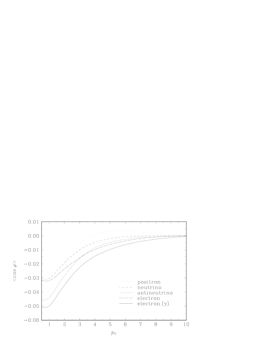
FIG. 2.: $\langle\cos\phi\rangle$ versus $p_{c}$ in inclusive processes. The leptons listed are the incoming leptons for charged weak-current processes. The last one with $\gamma$ is from the $ep$ scattering with a photon exchange.

In the semi-inclusive processes in which we tag a final-state charged pion, we use analytic fragmentation functions for simplicity. This is in contrast with studies using Monte Carlo simulation for the hadronization process[10]. In our numerical analysis we use Sehgal’s parametrization[11]. Sehgal’s parametrization for the quark fragmentation functions to pions is given by

$$D_{j}^{\pi}(z)=\frac{1}{z}\Bigl{(}0.05+1.05(1-z)^{2}\Bigr{)},$$ (122)

for $j=u,d,\overline{u},\overline{d}$ and $D_{j}^{\pi}(z)=0$ for other quarks. The gluon fragmentation function to pions is given by

$$D_{g}^{\pi}(z)=-0.1-2.1z+\frac{2.2}{z}+4.2\log z.$$ (123)

Note that the gluon fragmentation function is “softer” than the quark fragmentation functions, that is, $D_{g}^{\pi}(z)<D_{j}^{\pi}(z)$ for $z>0.21$. This functional form for the gluon is obtained by assuming that the gluon first breaks up into a quark-antiquark pair, and then the quarks fragment into the observed hadrons. At large $z$, the hadrons mainly come from quark fragmentation. For the sake of simplicity, we also nelgect the QCD-induced scale dependence of these fragmentation functions. The variation of the fragmentation function due to the scale dependence largely cancels out in the ratio defining $\langle\cos\phi\rangle$.

Since $Q^{2}=2ME_{l}x_{H}y$, where $M$ is the proton mass, $E_{l}$ is the energy of the incoming lepton in the proton rest frame, when we integrate over $x_{H}$ and $y$, the strong coupling constant $\alpha_{s}(Q^{2})$ should also be included in the integrands in the definition of $\langle\cos\phi\rangle$. The running coupling constant $\alpha_{s}$ has the $Q$ dependence as

$$\alpha_{s}(Q^{2})=\frac{12\pi}{(33-2n_{f})\ln(Q^{2}/\Lambda^{2})},$$ (124)

where $n_{f}$ is the number of quark flavors whose masses are below $Q$. However the inclusion of $\alpha_{s}(Q^{2})$ in the integrand is numerically negligible since it appears both in the numerator and in the denominator. Therefore in our analysis we do not include $\alpha_{s}(Q^{2})$ in the integrands. The numerical error in neglecting the variation of $\alpha_{s}$ with respect to $Q$ is less than a few percent.

TABLE II.: $\langle\cos\phi\rangle$ as a function of the transverse momentum cutoff $p_{c}$ for the semi-inclusive processes with a final-state charged pion. The last column is from the $ep$ scattering with a photon exchange. The kinematic range is $0.05\leq x_{H}\leq 0.3$, $0.2\leq y\leq 0.8$ and $0.3\leq z_{H}\leq 1.0$ with $Q\geq 2$ GeV.

$p_{c}$ (GeV)	$\nu\rightarrow e$	$e\rightarrow\nu$	$\overline{\nu}\rightarrow e^{+}$	$e^{+}\rightarrow\overline{\nu}$	$e\rightarrow e(\gamma)$
2.0	$-0.0515$	$-0.0591$	$-0.115$	$-0.0817$	$-0.0832$
3.0	$-0.0443$	$-0.0529$	$-0.128$	$-0.0854$	$-0.0805$
4.0	$-0.0399$	$-0.0482$	$-0.146$	$-0.0970$	$-0.0783$
5.0	$-0.0364$	$-0.0439$	$-0.166$	$-0.111$	$-0.0762$
6.0	$-0.0341$	$-0.0405$	$-0.187$	$-0.127$	$-0.0740$
7.0	$-0.0311$	$-0.0366$	$-0.204$	$-0.141$	$-0.0720$
8.0	$-0.0289$	$-0.0332$	$-0.219$	$-0.156$	$-0.0698$
9.0	$-0.0256$	$-0.0292$	$-0.224$	$-0.163$	$-0.0660$
10.0	$-0.0224$	$-0.0248$	$-0.226$	$-0.173$	$-0.0634$

FIG. 3.: $\langle\cos\phi\rangle$ versus $p_{c}$ in semi-inclusive processes. The leptons listed are the incoming leptons for charged weak-current processes. The last one with $\gamma$ is from the $ep$ scattering with a photon exchange.

The numerical results for the semi-inclusive processes are given in Table 2 and the plot is shown in Fig. 3. The numerical values are obtained by integrating over the same range as in the analysis of inclusive processes, $0.05\leq x_{H}\leq 0.3$, $0.2\leq y\leq 0.8$ and $0.3\leq z_{H}\leq 1.0$ with $Q\geq 2$ GeV. The azimuthal correlation in semi-inclusive processes shows a rich structure. As $p_{c}$ increases, $\langle\cos\phi\rangle$ decreases for the incoming antineutrino or the positron. On the other hand, for the incoming neutrino or the electron, it increases and approaches zero. The result from the $ep$ scattering with a photon exchange is located between these two cases. This behavior will be analyzed in detail in the next section and we compare it to the behavior in inclusive processes.

V Discussion

The most interesting feature of our analysis is the behavior of $\langle\cos\phi\rangle$ as a function of the transverse momentum cutoff $p_{c}$. Let us compare inclusive and semi-inclusive cases shown in Figs. 2 and 3 respectively. In inclusive processes $\langle\cos\phi\rangle$ approaches zero as $p_{c}$ increases irrespective of the incoming leptons. On the other hand, $\langle\cos\phi\rangle$ in semi-inclusive processes is numerically large compared to that in inclusive processes by an order of magnitude and it depends on the incoming leptons. However $\langle\cos\phi\rangle$ remains consistently negative in semi-inclusive processes. Negative values of $\langle\cos\phi\rangle$ mean that the final-state particles tend to be emitted to the direction of the incoming lepton.

We can understand why there is such asymmetry at order $\alpha_{s}$ in the context of color coherence at parton level as noted in Ref. [7]. When a quark-antiquark pair is produced in a color-singlet state, soft gluons tend to be emitted inside the cone defined by the quark-antiquark pair. In our case, we have an incoming quark and an outgoing quark. However we can regard the incoming quark as an outgoing antiquark and the pair as a color singlet. Therefore the configuration in which the outgoing quark is closer to the incoming lepton and a gluon is emitted between the incoming quark and the outgoing quark is more probable. It is this configuration that gives negative $\langle\cos\phi\rangle$ after boosting to the photon-proton center-of-mass frame assuming that we are in a kinematic regime where the observed hadron is coming from the fragmentation of the quark.

In the semi-inclusive processes in which we identify a final-state hadron, for example, a charged pion, note that the gluon fragmentation function is much softer than the quark fragmentation functions. That is, the gluon fragmentation function $D_{g}^{\pi}(z_{H}/z)$ decreases rapidly as $z_{H}/z\rightarrow 1$ compared to the quark fragmentation functions. This is clearly seen in Sehgal’s parametrization of the fragmentation functions. Therefore for large $z_{H}$ ($z_{H}\geq 0.3$ in our numerical result) we effectively pick up the pions which are fragments of quarks. This is exactly the situation where color coherence can explain the asymmetry. Of course, final-state quarks can be produced from the gluon-$W$ fusion. But in this case $\langle\cos\phi\rangle$ can be either positive or negative, hence there is a partial cancellation for wide ranges of $x_{H}$ and $z_{H}$.

In inclusive processes, since there appear no fragmentation functions, both quarks and gluons contribute to the asymmetry. But their contributions tend to cancel each other since the final-state particles are emitted in the opposite direction. Note the opposite signs in the pairs of terms ($A_{\nu}$, $B_{\nu}$), ($C_{\nu}$, $D_{\nu}$) and ($E_{\nu}$, $F_{\nu}$) in Eq. (54). However the asymmetry can arise depending on the kinematic range. For example, the valence quarks contribute dominantly for large $x_{H}/x$ because the valence quark distribution functions $F_{i}(x_{H}/x,Q^{2})$ are larger than other distribution functions. If we compare Figs. 2 and 3, the cancellation in inclusive processes is illustrated clearly. The magnitudes of $\langle\cos\phi\rangle$ in inclusive processes (Fig. 2) are smaller by an order of magnitude than those in semi-inclusive processes (Fig. 3).

Now let us consider the detailed behavior of $\langle\cos\phi\rangle$ as $p_{c}$ varies. In evaluating $\langle\cos\phi\rangle$, there are different combinations of parton distribution functions (and fragmentation functions in semi-inclusive processes) for different incoming leptons. However, since these functions appear both in the denominator and in the numerator, the main difference results from the matrix elements squared for each process. As the matrix elements squared for the incoming electron and for the incoming neutrino are proportional to each other, we expect that the behavior of $\langle\cos\phi\rangle$ from an incoming electron and from an incoming neutrino is similar though the magnitudes may be different. This is true for the cases with an incoming positron and an incoming antineutrino. This expectation is shown in Fig. 3 for semi-inclusive processes. It is not clear in Fig. 2 for inclusive processes since the magnitudes of $\langle\cos\phi\rangle$ are numerically too small to draw any conclusion.

One interesting feature in Fig. 3 is that when the incoming particle is an antineutrino or a positron, $\langle\cos\phi\rangle$ is more negative compared to the case of the incoming neutrino or electron. $\langle\cos\phi\rangle$ decreases as $p_{c}$ increases for incoming antileptons, while it increases and approaches zero for incoming leptons. This behavior results from complicated functions depending on $x$, $y$, $z$, $x_{H}$ and $z_{H}$. Therefore it is difficult to explain the behavior in a simple way. However we can explain why $\langle\cos\phi\rangle$ is more negative for incoming antileptons with large $p_{c}$.

In semi-inclusive processes, since we select the hadron with transverse momentum $P_{T}$ larger than the transverse momentum cutoff $p_{c}$, we have the relation

$$P_{T}^{2}=\frac{(1-x)(1-z)}{xz}z_{H}^{2}Q^{2}=2ME_{l}x_{H}y\frac{(1-x)(1-z)}{xz}z_{H}^{2}\geq p_{c}^{2}.$$ (125)

The second equality in Eq. (125) is obtained by the relation $Q^{2}=2x_{H}yME_{l}$. For large $p_{c}$, the phase space is confined to the region with small $x$, $z$ and large $x_{H}$, $y$ and $z_{H}$. In this region the ratio $z_{H}/z$, which appears in the fragmentation functions, is large, hence the contribution of the gluon fragmentation is negligible compared to that of the quark (antiquark) fragmentation. In other words $b_{\nu}$, $d_{\nu}$ in Eq. (109) and $b_{\nu}^{\prime}$, $d_{\nu}^{\prime}$ in Eq. (121) are negligible compared to other contributions. Similarly large $x_{H}/x$, which appears in the parton distribution functions, is preferred hence the contribution of the distribution functions of sea quarks and gluons is small compared to that of the valence quark distribution functions since the valence quark distribution functions are dominant for large $x_{H}/x$. As a result $c_{\nu}$, $e_{\nu}$, $f_{\nu}$ terms in (109) and $c_{\nu}^{\prime}$, $e_{\nu}^{\prime}$, $f_{\nu}^{\prime}$ terms in Eq. (121) are negligible. Therefore $a_{\nu}$ and $a_{\nu}^{\prime}$ dominate for large $p_{c}$. It means that the main contribution to $\langle\cos\phi\rangle$ comes from the scattering of an initial valence quark into a final-state quark, fragmenting to the observed pion.

Note that, since the parton distribution functions and the fragmentation functions appear both in the numerator and in the denominator, $\langle\cos\phi\rangle$ is mainly affected by the partonic scattering cross sections, which are functions of parton variables $x$, $y$ and $z$. For small $x$, $z$ and large $y$, only the first term in $a_{\nu}^{\prime}$ in the denominator and the first term in $a_{\nu}$ in the numerator are important. The partonic part of the integrand in the denominator behaves as $(xz)^{-1}$ and that in the numerator behaves as $-(xz)^{-1/2}(1-y)^{3/2}$. Since the integrand in the denominator grows faster than that of the numerator for small $x$, $z$ and large $y$, $\langle\cos\phi\rangle$ in semi-inclusive processes approaches zero for the incoming electron or neutrino for large $p_{c}$, but it remains negative.

In the case of the incoming antineutrino, $a_{\overline{\nu}}$ and $a_{\overline{\nu}}^{\prime}$ terms are dominant for large $p_{c}$ as in the case with the incoming neutrino. But the behavior of these terms are different. Though we do not present the forms of $a_{\overline{\nu}}$ and $a_{\overline{\nu}}^{\prime}$ here, we can see the dependence of $a_{\overline{\nu}}$ and $a_{\overline{\nu}}^{\prime}$ on the partonic variables $x$, $y$ and $z$ in Eqs. (81) and (93) for inclusive processes since the partonic cross sections are the same. For small $x$, $z$ and large $y$, only the third term in the denominator survives and it behaves as $(xz)^{-1}$. On the other hand, the integrand in the numerator behaves as $-(xz)^{-1/2}(1-y)^{1/2}$. Therefore the magnitude of $\langle\cos\phi\rangle$ is larger than that for the incoming electron or neutrino by a factor of $(1-y)^{-1}$ in the integrand in the numerator, hence $\langle\cos\phi\rangle$ is more negative than the case of an incoming electron or neutrino. In addition, because of this factor $(1-y)^{-1}$, the difference of $\langle\cos\phi\rangle$ between the incoming antineutrino and the incoming positron is larger than that for the incoming electron and and the incoming neutrino. It is also interesting to note that the azimuthal asymmetry exhibited by a photon exchange in the semi-inclusive $ep$ scattering is intermediate between the two cases in which there are leptons or antileptons.

The behavior of $\langle\cos\phi\rangle$ in inclusive processes can be explained by the same argument. In this case we identify the transverse momentum of the final-state hadron (or a jet) as the transverse momentum of the scattered parton. It corresponds to setting $z_{H}=z$. Therefore we select the final-state particle with the momentum cutoff $p_{c}$ satisfying

$$P_{T}^{2}=\frac{z(1-z)(1-x)}{x}Q^{2}=2ME_{l}x_{H}y\frac{z(1-z)(1-x)}{x}\geq p_{c}^{2}.$$ (126)

Therefore as $p_{c}$ gets large, the integrated phase space is confined to a region with small $x$, large $x_{H}$, $y$ and intermediate $z$ between 0 and 1. Since the variable $x_{H}/x$ in the parton distribution functions is large, the contribution from the gluon distribution function is negligible. This means that $E$ and $F$ in Eqs. (54) and (81) and $E^{\prime}$, $F^{\prime}$ in Eqs. (69) and (93) can be neglected. Therefore remaining $A$, $B$, $C$ and $D$ terms and their primed quantities contribute to $\langle\cos\phi\rangle$.

As we can see in Eq. (57), the integrands in the denominator behave as $x^{-1}$ whether the incoming particle is a neutrino or an antineutrino. In the case of the neutrino, the integrand in the numerator from $A_{\nu}$, $B_{\nu}$ terms behaves as $x^{-1/2}(1-y)^{3/2}$, while it behaves as $x^{-1/2}(1-y)^{1/2}$ from $C_{\nu}$, $D_{\nu}$ terms. These terms are smaller than the integrands in the denominator. Furthermore there is a partial cancellation between $A_{\nu}$ and $B_{\nu}$ because they have opposite signs. This is also true for $C_{\nu}$ and $D_{\nu}$. Therefore $\langle\cos\phi\rangle$ becomes very small. The same argument applies to the case of the incoming antineutrino.

As $p_{c}$ gets large, the azimuthal asymmetry tends to be washed out in inclusive processes. This behavior of $\langle\cos\phi\rangle$ is expected considering the momentum conservation. In our case in which there are two outgoing particles in the $W$-proton frame, the transverse momentum of one particle is balanced by another particle emitted in the opposite direction. Therefore if we sum over all the contributions from all the emitted particles, there should be no azimuthal asymmetry. The small azimuthal asymmetry, as shown in Fig. 2, arises since we do not include all the emitted particles with the given choice of $x_{H}$, $y$ and $z_{H}$.

VI Conclusion

We have extensively analyzed the azimuthal correlation of final-state particles in charged weak-current processes. It is a clean test of perturbative QCD if we make the transverse momentum cutoff $p_{c}$ larger than, say, 2 GeV. It turns out that the azimuthal asymmetry is appreciable in semi-inclusive processes compared to inclusive processes since the asymmetry mainly comes from the contribution of an final-state quark due to the soft nature of the gluon fragmentation function for large $z_{H}$. In inclusive processes we sum over all the contributions from quarks (antiquarks) and gluons, and the sum approaches zero as we include a wider range of variables due to the momentum conservation.

In addition the azimuthal asymmetry is more conspicuous for semi-inclusive processes with an incoming antineutrino or a positron. Previously there was an attempt to analyze the azimuthal asymmetry at HERA in $ep$ scattering for electroproduction via a photon exchange. However since $e^{+}p$ scattering has been performed at HERA, we expect that the test of the azimuthal asymmetry is more feasible because the magnitude of $\langle\cos\phi\rangle$ is bigger in semi-inclusive processes with an incoming positron. In CCFR experiments they consider only the inclusive cross section for $\nu_{\mu}\ (\overline{\nu}_{\mu})+H\rightarrow\mu\ (\mu^{+})+X$, where $H$ is the target hadron. If they are able to identify a final-state hadron, they will also be able to observe the azimuthal correlations in various charged weak-current processes.

The azimuthal asymmetry in lepton-hadron scattering results from a combination of main ideas in the QCD-improved parton model. As mentioned above, the parton model states that the hadronic cross section can be separated into three parts: the parton distribution functions, the fragmentation functions and the partonic hard scattering cross section. Each element contributes to the azimuthal asymmetry. If we make a transverse momentum cutoff $p_{c}$ large enough in order for perturbative QCD to be valid, the small-$x$ (large-$x_{H}/x$) region mainly contributes, hence the contribution from valence quarks is dominant. At the same time, large $p_{c}$ implies that the small-$z$ (large-$z_{H}/z$) region mainly contributes to the asymmetry. This means that quark or antiquark fragmentation functions contribute dominantly. The detailed behavior of $\langle\cos\phi\rangle$ depends on the hard scattering cross section at parton level. Therefore the experimental analysis of the azimuthal asymmetry tests the very basic ideas in the QCD-improved parton model.

REFERENCES

[1] H. Georgi and H.D. Politzer, Phys. Rev. Lett. 40, 3 (1978).
[4] P. Mazzanti, R. Odorico and V. Roberto,
Phys. Lett. B80, 111 (1978).
[5] Electron Muon Collaboration, Z. Phys. C34, 277
(1987).
[6] See, for example, A. Méndez, Nucl. Phys. B145, 199 (1978); A. Méndez, A. Raychaudhuri and V.J. Stenger,
Nucl. Phys. B148, 499 (1979).
[7] J. Chay, S.D. Ellis and W.J. Stirling, Phys. Lett. B269, 175 (1991); Phys. Rev. D45, 46 (1992).
[8] See, for example, J.E. Huth et al., in Research Directions for the Decade, Proceedings of the Summer Study
on High Energy Physics, Snowmass, Colorado, 1990, edited by
E.L. Berger (World Scientific, Singapore, 1991).
[9] A.D. Martin, R.G. Roberts and W.J. Stirling,
Phys. Rev. D50, 6734 (1994).
[10] See, for example, A. König and P. Kroll,
Z. Phys. C16, 89 (1982).
[11] L.M. Sehgal, in Proceedings of the 1977
International Symposium on Lepton and Photon Interactions at High
Energies, ed. F. Gutbrod (DESY, 1977), Hamburg, p.837.