Abstract

We discuss the general operator product expansion of a non-forward unequal mass virtual compton scattering scattering amplitude. We find that the expansion now should be done in double moments with new moment variables. There are in the expansion new sets of leading twist operators which have overall derivatives, and they mix under renormalization. We compute the evolution kernels from which the anomalous dimensions for these operators can be extracted. We also obtain the lowest order Wilson Coefficients. In the high energy limit we find the explicit form of the dominant contributing anomalous dimensions and solve the resulting renormalization group equation. We find the same high energy behavior as indicated by the conventional double leading logarithmic analysis.

PACS number(s): 12.38.Bx, 13.60.-r, 11.10.Gh

I Introduction

Recently there is much interest in the analysis of non-forward scattering processes, for example, Deeply Virtual Compton Scattering (DVCS) [2, 3] and hard diffractive electroproduction of vector mesons [4, 5, 6, 7] in Deeply Inelastic Scattering (DIS).

Ji [2, 8] proposed that one can obtain from DVCS information on the Off-Forward Parton Distributions (OFPD) which in this case contain new information on long distance physics. He studied their evolution and sum rules (in terms of form factors) and obtained certain estimates at low energy. Radyushkin also studied the scaling limit of DVCS [3], and generalized the discussion to hard exclusive electroproduction processes [5, 9]. The non-perturbative information is incorporated in his double distributions $F(x,y;t)$ and non-forward distribution functions $F_{\zeta}(X;t)$. He discussed their spectral properties, the evolution equations they satisfy, their basic uses and general aspects of factorization for hard exclusive processes. A third parametrization for the non-perturbative information was proposed by Collins et al. [6, 7]. They performed a numerical study of their non-diagonal parton distributions in leading logarithmic approximation, in which they found the nondiagonal gluon distribution $x_{2}G(x_{1},x_{2},Q^{2})$ can be well approximated at small x by the conventional gluon density $xG(x,Q^{2})$.

In this paper, we formulate a general operator product expansion description for a generic non-forward unequal mass virtue compton scattering amplitude(see Fig. 1). Because of the non zero momentum transfer $r=p-p^{\prime}$ from the initial state proton to the final state proton, the scaling behavior must be different from that in a forward case because of the new kinematic degree of freedom (the non-forwardness). Indeed we will show that compared with forward scattering one has two scaling variables, or equivalently, two moment variables $\omega$ and $\nu$ (see (12)). The amplitude should now be expanded in terms of double moments with respect to them. There are associated with these double moments new sets of operators that have overall derivatives in front (see (III)), which mix among themselves under renormalization via an anomalous dimension matrix. The reduced non-forward matrix elements of these operators are thus double distribution functions, but they do not seem to have a simple probability interpretation. We will focus our attention on the high energy behavior of these distribution functions, solving their renormalization group equations, and show that in the high energy limit the gluonic double distribution function actually reduces to the conventional (forward) gluon density and the high energy behavior is the same as obtained by a conventional double leading logarithmic (DLL) analysis.

The outline of the paper is as follows. In Section II we define the process and the kinematics of the non-forward scattering amplitude ${\rm T}_{\mu\nu}$. A general tensorial decomposition of ${\rm T}_{\mu\nu}$ into invariant amplitudes is given. In Section III we perform a general operator product expansion of ${\rm T}_{\mu\nu}$, define new moment variables and give their relationship to the more conventional Bjorken type scaling variables. In Section IV we write down the renormalization group equations, present the equivalence of evolution kernels for the double moments, and calculate explicitly the lowest order Wilson Coefficients. In Section V we go to the high energy limit to solve the renormalization group equations and make connection with the DLL analysis. Section VI gives conclusions and outlook for future work.

II Decomposition of the Amplitude

Consider an unequal mass (non-forward) virtue compton scattering amplitude ${\rm T}_{\mu\nu}$ as shown in Fig.1, where the incoming photon $q^{\prime}=q-r$ and the outgoing one $q$ have different invariant masses:

$$q^{\prime 2}=-Q_{1}^{2},\,\,\,\,q^{2}=-Q_{2}^{2}$$ (1)

FIG. 1.: Non-forward Scattering Amplitude

We restrict our discussion to amplitudes. Cross sections are obtained from the square of the amplitudes. In the non-forward case there is not a simple optical-theorem relating the imaginary part of an amplitude to a cross section [11]. Our main interest is in the high energy limit, so similar to [4] we take all but one of the components of the proton momentum to be zero, same for the momentum transfer $r$. Thus $-t=r^{2}=0$, while $r$ is proportional to the external momentum $p$ and

$$r=\zeta p,\,\,\,\,\,\,\,\,\,\,\,\,\,\,\,\,{\rm with}\,\,\,\,\,\,\,\,\,\,\zeta=\frac{\,\,\,\,q^{2}-q^{\prime 2}}{2p\cdot q}\,\,\,.$$ (2)

We can write the spin averaged amplitude, up to an overall $\delta$-function in momentum space, as

$${\rm T}_{\mu\nu}(p,q^{\prime},q)=i\int d^{4}z\,e^{-i\bar{q}\cdot z}\,\langle{p^{\prime}}|T\,j_{\mu}(-{z\over 2})j_{\nu}({z\over 2})|{p}\rangle\,$$ (3)

where $\overline{q}={1\over 2}(q^{\prime}+q)$ and $-\overline{q}^{2}={1\over 2}(Q_{1}^{2}+Q_{2}^{2})\equiv\overline{Q}^{2}$ is now the ’natural’ scale of the scattering process. DIS corresponds to $q=q^{\prime}$ while DVCS corresponds to $q^{2}=0$. We always suppose $Q_{2}^{2}\leq Q_{1}^{2}$ so that $\zeta\geq 0$.

Use translation operator one can prove that the conservation of the electro$\!-\!$magnetic current now requires the amplitude to satisfy

$$q^{\mu}{\rm T}_{\mu\nu}=0;\,\,\,\,\,q^{\prime\nu}{\rm T}_{\mu\nu}=0.$$ (4)

${\rm T}_{\mu\nu}$ is no longer symmetric, rather it is invariant under $\mu\leftrightarrow\nu,\,\,\,q\leftrightarrow-q^{\prime}$. Together with current conservation (4), we obtain the general tensorial decomposition of ${\rm T}_{\mu\nu}$ as

$${1\over{\sqrt{1-\zeta}}}{\rm T}_{\mu\nu}=\left(-g_{\mu\nu}+\frac{q^{\prime}_{\mu}q_{\nu}}{\overline{q}^{2}}\right){\rm T_{1}}+{1\over M^{2}}\left(p_{\mu}p_{\nu}-\frac{p\cdot q}{\overline{q}^{2}}(p_{\mu}q_{\nu}+q^{\prime}_{\mu}p_{\nu})+(\frac{p\cdot q}{\overline{q}^{2}})^{2}q^{\prime}_{\mu}q_{\nu}\right){\rm T_{2}},$$ (5)

where ${\rm T_{i}}={\rm T_{i}}(q^{\prime 2},q^{2},p\cdot q)$ are invariant amplitudes analogous to those in DIS and they are even functions of $p\cdot q$. We have pulled out from them an explicit factor of $\sqrt{1-\zeta}$ coming from the external spinors as was done in, e.g. ,[3]. Note we still have only two independent invariant amplitudes even in the presence of three invariants, instead of two as in the forward case.

III Operator Product Expansion

In the short distance limit, we can perform an OPE for ${\rm T}_{\mu\nu}$ as a sum of products of local operators and their corresponding Wilson Coefficients [12]:

$$T\,j_{\mu}(-{z\over 2})j_{\nu}({z\over 2})\stackrel{{\scriptstyle z_{\mu}\rightarrow 0}}{{\longrightarrow}}\hat{A}_{\mu\nu}\,\sum_{J=1}^{\infty}\sum_{n=0}^{J}\sum_{i=1}^{u_{J}}\,F_{J,n}^{(i)}(z^{2})\hat{O}_{\mu_{1}...\mu_{J}}^{(i)(J,n)}(0){z\over 2}^{\mu_{1}}...{z\over 2}^{\mu_{J}}$$ (6)

$$+\hat{B}_{\mu\nu\alpha\beta}\sum_{J=1}^{\infty}\sum_{n=0}^{J}\sum_{i=1}^{u_{J}}\,E_{J,n}^{(i)}(z^{2})\hat{O}_{\alpha\beta;\mu_{1}...\mu_{J}}^{(i)(J,n)}(0){z\over 2}^{\mu_{1}}...{z\over 2}^{\mu_{J}},$$ (7)

where $\hat{A}_{\mu\nu}$ and $\hat{B}_{\mu\nu\alpha\beta}$ are conserved tensor structure operators and all indices except $\mu,\nu$ are symmetrized as usual. $\hat{B}_{\mu\nu\alpha\beta}$ is the same as in the forward case, i.e. ,

$$\hat{B}_{\mu\nu\alpha\beta}=g_{\mu\alpha}g_{\nu\beta}\Box+g_{\mu\nu}\partial_{\alpha}\partial_{\beta}-g_{\mu\alpha}\partial_{\nu}\partial_{\beta}-g_{\nu\beta}\partial_{\mu}\partial_{\alpha}\,,$$ (8)

and corresponds to the tensor structure multiplying ${\rm T}_{2}$ in (5) while we have not found the explicit form of $\hat{A}_{\mu\nu}$ which would generate the tensor structure corresponding to ${\rm T}_{1}$. But, as in the forward case, once we know ${\rm T}_{2}$, we can obtain ${\rm T}_{1}$ by a Callen-Gross relationship, at least in leading logarithmic level (see (22)).

Because now the momentum flowing into the local vertex is $r$ instead of zero, we have to include in the expansion new sets of operators that have overall derivatives. In leading twist (the meaning of which in this case will be clear later) the operators for QCD are

$$\hat{O}_{\mu_{1}...\mu_{J}}^{(q)(J,n)} = \partial_{\mu_{1}}...\partial_{\mu_{n}}\,\tilde{q}(0)\gamma_{\mu_{n+1}}i\stackrel{{\scriptstyle\leftrightarrow}}{{\cal D}}_{\mu_{n+2}}...i\stackrel{{\scriptstyle\leftrightarrow}}{{\cal D}}_{\mu_{J}}q(0)$$ (10)

$$\hat{O}_{\mu_{1}...\mu_{J}}^{(g)(J,n)} = \partial_{\mu_{1}}...\partial_{\mu_{n}}\,F_{\mu_{n+1}}^{\,\,\,\,\,\,\,\,\nu}(0)i\stackrel{{\scriptstyle\leftrightarrow}}{{\cal D}}_{\mu_{n+1}}...i\stackrel{{\scriptstyle\leftrightarrow}}{{\cal D}}_{\mu_{J}}F_{\mu_{J}\nu}(0).$$ (11)

After taking the matrix elements between the asymmetric external states, and after taking a Fourier transform, the external derivatives would eventually be turned into factors of $r_{\mu}$ while the internal derivatives into either $r_{\mu}$ or $(p+p^{\prime})_{\mu}\equiv(2p-r)_{\mu}$. We thus define the two moment variables in the non-forward case as

$$\omega=\frac{(2p-r)\cdot q}{{\overline{Q}}^{2}},\,\,\,\,\,\,\,\,\,\,\,\,\nu=\frac{r\cdot q}{{\overline{Q}}^{2}}\,\,.$$ (12)

The forward case would be the limit $\nu=0$ while DVCS corresponds to $\nu=1$.

In a QCD-parton picture, the diagrams contributing to ${\rm T}_{\mu\nu}$ are the so-called ’hand-bag’ diagrams as shown in Fig.2. If we parametrize the momentum of the scattered parton as $k=xp+yr$ (see, e.g.[3]), where $x$ and $y$ are two Bjorken type scaling variables conjugate to $\tilde{\omega}\equiv{{2p\cdot q}/Q_{1}^{2}}$ and $\tilde{\nu}\equiv{{2r\cdot q}/Q_{1}^{2}}$, respectively, our moment variables are related to these quantities via

$$\omega={Q_{1}^{2}\over\overline{Q}^{2}}(x\tilde{\omega}+y\tilde{\nu}-{1\over 2}\tilde{\nu})\,\,\,;\,\,\,\,\,\,\,\,\,\,\,\,\,\,\,\,\,\,\,\,\,\,\,\,\nu={Q_{1}^{2}\over\overline{Q}^{2}}({1\over 2}\tilde{\nu}).$$ (13)

FIG. 2.: Handbag Diagrams in QCD-Parton Picture

There will be mixing between operators with same $J$ but different $n$ labels. To be more specific, evolution in $\overline{Q}^{2}$ will lead to mixing from $\hat{O}^{(i)(J,n)}$ to $\hat{O}^{(i)(J,n^{\prime})}$ with $0\leq n\leq n^{\prime}\leq J$. But we do have the freedom to choose, for simplification, at the factorization scale $\mu_{0}$, that all internal derivatives give factors of $(2p-r)$. Thus we can write

$${\langle{p^{\prime}}|\hat{O}_{\mu_{1}...\mu_{J}}^{(i)(J,n)}|{p}\rangle}_{(\mu_{0})}=r_{\mu_{1}}...r_{\mu_{n}}(2p-r)_{\mu_{n+1}}...(2p-r)_{\mu_{J}}\,{\langle{p^{\prime}}||\hat{O}^{(i)(J,n)}||{p}\rangle}_{(\mu_{0})}$$ (14)

and the reduced matrix elements will depend only on $J-n$:

$${\langle{p^{\prime}}||\hat{O}^{(i)(J,n)}||{p}\rangle}={\langle{p^{\prime}}||\hat{O}^{(i)(J-n,0)}||{p}\rangle}\,\,\,.$$ (15)

Analogous to the forward case, taking the logarithmic derivative of $\overline{q}^{2}$ of the Fourier transformed Wilson Coefficients $E$ we define the Wilson Coefficients in momentum space $\tilde{E}$ as

$${{p\cdot q}\over\overline{Q}^{2}}i({1\over\overline{q}^{2}})^{2}\tilde{E}_{J,n}^{(i)}=(-i\overline{q}^{2}{\partial\over{\partial\overline{q}^{2}}})^{J}\int d^{4}z\,e^{-i\bar{q}\cdot z}E_{J,n}^{(i)},$$ (16)

where we have pulled out an explicit factor of ${{p\cdot q}\over\overline{Q}^{2}}$ to make the form of $\tilde{E}$ simple (see (IV C)). We have

$${\rm T}_{\mu\nu} = i^{2}\sum_{J,n,i}{\langle{p^{\prime}}||\hat{O}^{(i)(J,n)}||{p}\rangle}_{(\mu_{0})}\omega^{J\!-\!n}\nu^{n}\left((-g_{\mu\nu}+\frac{q^{\prime}_{\mu}q_{\nu}}{\overline{q}^{2}})\,{{p\!\cdot\!q}\over\overline{Q}^{2}}\,\tilde{F^{\prime}}_{J,n}^{(i)}(\alpha_{s},{\overline{Q}\over{\mu_{0}}})\right.$$ (18)

$$\left.+{1\over{p\!\cdot\!q}}\left(p_{\mu}p_{\nu}-\frac{p\!\cdot\!q}{\overline{q}^{2}}(p_{\mu}q_{\nu}+q^{\prime}_{\mu}p_{\nu})+(\frac{p\cdot q}{\overline{q}^{2}})^{2}q^{\prime}_{\mu}q_{\nu}\right)\tilde{E}_{J\!-\!2,n}^{(i)}(\alpha_{s},{\overline{Q}\over\mu_{0}})\right).$$

$\tilde{F^{\prime}}$ is a combination of $\tilde{E}$ and a similarly defined $\tilde{F}$. Note we have explicitly indicated their dependence on the factorization scale. Non-leading twist terms in this case are suppressed by a power of ${1\over{\overline{Q}^{2}}}$. Thus we obtain the invariant amplitudes as follows:

$$\sqrt{1-\zeta}\,{\rm T}_{1}=-\sum_{J,n,i}{\langle{p^{\prime}}||\hat{O}^{(i)(J,n)}||{p}\rangle}_{(\mu_{0})}\omega^{J\!-\!n}\nu^{n}\tilde{F^{\prime}}_{J,n}^{(i)}(\alpha_{s},{\overline{Q}\over\mu_{0}})\,\,\,\,\,\,\,\,\,\,\,\,\,\,\,\,\,\,\,\,\,\,\,\,\,$$ (20)

$${{p\!\cdot\!q}\over M^{2}}\sqrt{1-\zeta}\,{\rm T}_{2}=-\sum_{J,n,i}{\langle{p^{\prime}}||\hat{O}^{(i)(J,n)}||{p}\rangle}_{(\mu_{0})}\omega^{J\!-\!n}\nu^{n}\tilde{E}_{J-2,n}^{(i)}(\alpha_{s},{\overline{Q}\over\mu_{0}})\,\,\,.\,\,\,\,\,\,\,\,\,$$ (21)

IV Renormalization Group Equation and Anomalous Dimensions

A Renormalization Group Equation

We concentrate on ${\rm T}_{2}$. ${\rm T}_{1}$ can be obtained, as in the case of a forward scattering, from the Callen-Gross relationship

$${\rm T}_{1}={{p\cdot q}\over{M^{2}}}{\rm T}_{2}$$ (22)

${\rm T}_{2}$ can be regarded as a double distribution function and is the sum of ’double’ moments

$${\rm T}_{2}=\sum_{J,n}\omega^{J-n}\nu^{n}{\rm T}_{2}^{(J,n)},$$ (23)

with the double moments ${\rm T}_{2}^{(J,n)}$ as

$$\sqrt{1-\zeta}{{p\!\cdot\!q}\over M^{2}}{\rm T}^{(J,n)}_{2,(\overline{Q},\mu_{0})}=-\sum_{i}{\langle{p^{\prime}}||\hat{O}^{(i)(J,n)}||{p}\rangle}_{(\mu_{0})}\tilde{E}_{J-2,n}^{(i)}(\alpha_{s},{\overline{Q}\over\mu_{0}})$$ (24)

We will eventually analytically continue in $J$, but leave $n$ as discrete. The inverse of expansion (23) is

$${\rm T}_{2}^{(J,n)}=\int_{c}{{d\omega}\over\omega}\int_{c}{{d\nu}\over\nu}\,({1\over\omega})^{J\!-\!n}({1\over\nu})^{n}{\rm T}_{2}(\overline{Q}^{2},\omega,\nu)$$ (25)

$$=2i\int_{1}^{\infty}{{d\omega}\over\omega}\int_{c}{{d\nu}\over\nu}\,({1\over\omega})^{J\!-\!n}({1\over\nu})^{n}{\rm W}_{2}(\overline{Q}^{2},\omega,\nu)$$ (26)

where $c$ is any contour in the $\omega(\nu)$ plane that encloses the origin and ${\rm W}_{2}={\rm Im\,T}_{2}$. Note in obtaining the second equality we have used the fact that ${\rm T}_{2}$ is even in $\omega$. ${\rm T}_{2}$ now as a double distribution function is given by

$${\rm T}_{2}(\overline{Q}^{2},\omega,\nu)=\int_{c}{{dJ}\over{2\pi i}}\sum_{n=0}^{\infty}e^{(J-n)\log\omega}\,\nu^{n}\,{\rm T}_{2}^{(J,n)}$$ (27)

with the contour $c$ lying parallel to the imaginary axis in the $J-n$ plane and to the right of all singularities in that plane.

Under renormalization, these operators scale according to a renormalization group equation

$$\mu^{2}{d\over{d\mu^{2}}}\hat{O}^{(i)(J,n)}=\sum_{n^{\prime}=n}^{J}\sum_{i^{\prime}}\tilde{\Gamma}_{nn^{\prime}}^{ii^{\prime}}\hat{O}^{(i^{\prime})(J,n^{\prime})}$$ (28)

where $\tilde{\Gamma}$ is the anomalous dimension matrix which is upper triangular and acts in the product space $J\otimes u_{J}$. The Wilson Coefficients then obey a similar renormalization group equation

$$\mu^{2}{d\over{d\mu^{2}}}\tilde{E}^{(i)}_{J,n}(\alpha_{s}(\mu),{\overline{Q}\over\mu})=-\sum_{n^{\prime}=0}^{n}\sum_{i^{\prime}}\tilde{E}^{(i^{\prime})}_{J,n^{\prime}}\,\,\,\tilde{\Gamma}_{n^{\prime}n}^{i^{\prime}i}.$$ (29)

We can write the solution as

$$\tilde{E}^{(i)}_{J,n}(\alpha_{s}(\mu),{\overline{Q}\over\mu})=\sum_{n^{\prime}=0}^{n}\sum_{i^{\prime}}\tilde{E}^{(i^{\prime})}_{J,n^{\prime}}(\alpha_{s}(\overline{Q}),1)\,\,\,{\rm M}_{n^{\prime}n}^{i^{\prime}i}(\alpha(\overline{Q}),{\overline{Q}\over\mu}),$$ (30)

where ${\rm M}$ is a path ordered exponential of the anomalous dimension matrix, formally given as

$${\rm M}_{n^{\prime}n}^{i^{\prime}i}(\alpha(\overline{Q}),{\overline{Q}\over\mu})=\left({\cal P}\exp(-\int_{\mu^{2}}^{\bar{Q}^{2}}\tilde{\Gamma}(\alpha_{s}(\lambda^{2})){{d\lambda^{2}}\over\lambda^{2}})\right)_{n^{\prime}n}^{i^{\prime}i}$$ (31)

Thus the double moments are given by

$$\sqrt{1-\zeta}{{p\!\cdot\!q}\over M^{2}}{\rm T}^{(J,n)}_{2,(\overline{Q},\mu_{0})}=-\sum_{n^{\prime}=0}^{n}\sum_{i^{\prime}i}\tilde{E}_{J-2,n^{\prime}}^{(i^{\prime})}(\alpha_{s},{\overline{Q}\over\mu_{0}})\,\,\,{\rm M}_{n^{\prime}n}^{i^{\prime}i}(\alpha(\overline{Q}),{\overline{Q}\over\mu_{0}})\,\,\,{\langle{p^{\prime}}||\hat{O}^{(i)(J,n)}||{p}\rangle}_{(\mu_{0})}.$$ (32)

B Anomalous Dimensions

In light-cone gauge, the lowest order anomalous dimensions of the quark and gluon operators are generated by the usual triangle diagrams (note: the graphs where we have more than two quark/gluon lines meet at the vertex are zero because of the gauge choice) as shown in Fig. 3

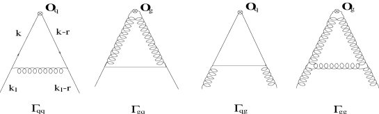
FIG. 3.: Triangle Graphs for the Anomalous Dimensions

Compute the graphs using light-cone variables with the definition

$$\omega={k_{+}\over k_{1+}},\,\,\,\,\,\nu={r_{+}\over k_{1+}},$$ (33)

and the conventions (cf. [13], also see Appendix A)

$$O_{q}^{(J,n)(+)}(k,k-r) = \gamma_{+}(2k-r)_{+}^{J\!-\!n\!-\!1}r_{+}^{n}$$ (35)

$$O_{g}^{(J,n)\alpha\beta}(k,k-r) = 2g_{\alpha\beta}\,n\cdot k\,n\cdot{(k-r)}\,(2k-r)_{+}^{J\!-\!n\!-\!2}r_{+}^{n}\,\,\,\,\,\,$$ (36)

where $n^{2}=0$ and $n\cdot A=A_{+}$ for any four vector $A$, yields (see Appendix A for details)

$$\Gamma_{qq}^{(\!+\!)}\! = \!{\alpha_{s}\over{2\pi}}C_{F}\,\gamma_{+}k_{1+}^{J-1}\nu^{n}\,\int_{0}^{1}d\omega\,(2\omega-\nu)^{J\!-\!n\!-\!1}\left(\Theta(\nu\!-\!\omega)\,{1\over\nu}\,\omega\,(1+{\nu\over{1-\omega}})\right.$$ (39)

$$\,\,\,\,\,\,\,\,\,\,\,\,\,\,\,\,\,\,\,\,\,\,\left.+\,\Theta(\omega\!-\!\nu){1\over{1\!-\!\nu}}{{1+\omega^{2}-\nu(1+\omega)}\over{1-\omega}}+\delta(1\!-\!\omega)(-\!2I_{0}-\log(1\!-\!\nu)+{3\over 2})\right)$$

$$\Gamma_{gq}^{(\!+\!)}\! = \!{\alpha_{s}\over{2\pi}}C_{F}\,\gamma_{+}k_{1+}^{J-1}\nu^{n}\!\int_{0}^{1}\!d\omega(2\!\omega\!-\!\nu)^{J\!-\!n\!-\!2}\left(\Theta(\nu\!-\!\omega){1\over\nu}(\omega^{2}\!-\!2\omega)\!-\!\Theta(\omega\!-\!\nu){1\over{1\!-\!\nu}}(1\!+\!(1\!-\!\omega)^{2}\!-\!\nu)\right),$$ (40)

$$\Gamma_{qg}^{ij}\! = \!{\alpha_{s}\over{2\pi}}{1\over 2}2g^{ij}k_{1\!+}^{J}\nu^{n}\!\int_{0}^{1}\!d\omega(2\!\omega\!-\!\nu)^{J\!-\!n\!-\!1}\!\left(\!-\!\Theta(\nu\!-\!\omega){1\over\nu}\omega(2\omega\!-\!1\!-\!\nu)\!+\Theta(\omega\!-\!\nu){1\over{1\!-\!\nu}}(\omega^{2}\!+\!(1\!-\!\omega)^{2}\!-\!\omega\!\nu)\!\right),$$ (41)

$$\Gamma_{gg}^{ij}\! = \!{{\alpha_{s}C_{A}}\over{2\pi}}2g^{ij}k_{1\!+}^{J}\nu^{n}\!\int_{0}^{1}\!\!d\omega(2\omega\!-\!\nu)^{J\!-\!n\!-\!2}\!\left(\!\Theta(\nu\!-\!\omega){1\over 2}({1\over\nu}(4\omega^{3}\!\!-\!\omega^{2}\!\!+\!4\omega)\!+\!({{\omega^{3}\!\!+\!\omega^{2}\!\!-\!2\omega^{2}\nu}\over{1-\omega}}\!-\!3(\omega^{2}\!+\!\omega)))\right.$$ (43)

$$\left.+{{\Theta(\omega\!-\!\nu)}\over{1\!-\!\nu}}({{2(1\!-\!\omega\!+\!\omega^{2})^{2}}\over{1-\omega}}\!+\!\nu\!{{\nu(1\!+\!\omega^{2})\!-\!2(1\!+\!\omega^{3})}\over{1-\omega}})\!+\!(1\!-\!\nu)\delta(1\!-\!\omega)(\!-\!2I_{0}\!-\!\log(1\!-\!\nu)\!+\!{b_{0}\over{2C_{A}}})\right).$$

We have included virtual corrections coming from the self-energy graphs that will cancel the colinear singularities at end point in the $\omega$ integration ($I_{0}$ terms, see (A13) for the definition of $I_{0}$) and give correct constant terms in the anomalous dimensions. $\Theta$ is the usual step function and $b_{0}=11-{2\over 3}n_{f}$ is the leading coefficient of the QCD $\beta$-function.

Some comments are in order. It is straightforward to show that in the forward limit where $\nu=0$, (IV B) reduces to the conventional Altarelli-Parisi splitting functions [14]. However, because of the non-forwardness, there is no simple probability interpretation for these evolution kernels as splitting functions.

The reason we have two terms for each triangle graph is that for different $k_{+}$ integration regions pinching of the $k_{-}$ pole is different (see Appendix A). Thus there is no straightforward optical-theorem type dispersion relationship between the cross section and the imaginary part of the amplitude. Nonetheless, we can still do analytic continuation in $J$ and relate the matrix elements to ’double parton distributions’ [11] which now may not have a direct probability interpretation. The second terms of our $\Gamma$ differ from those of [7] only because the factor $n\cdot k\,n\cdot(k-r)$ in our (IV Bb) is not included in the definition of their gluon vertices.

After we perform the $\omega$ ( i.e. $k_{+}$) integral, we can in principle obtain the corresponding anomalous dimension matrix in moment space. At first sight, the $(1-\nu)^{-1}$ factor of the second terms may generate a series of infinite sum over powers of $\nu$, which will spoil the locality of the vertex thus invalidate the operator product expansion. Detailed calculations show that because the lower bound of integration is now $\nu$ instead of zero, there will also always be at least one power of $(1-\nu)$ coming out from the integral. Furthermore, the highest powers of $\nu$ cancel completely between the first two terms of each $\Gamma$, leaving the highest surviving $\nu$ power as $\nu^{J-1}$ for the quark sector and $\nu^{J}$ for the gluonic sector, as must be the case to make the OPE valid. All the $I_{0}$ and $\log(1-\nu)$ terms also cancel completely between real and virtual graphs.

Because of the mixing among different $n$ moments, as well as between quark and gluon sectors, it is very difficult to read off the anomalous dimensions of the mixing between two operators (with same $J$) of definite $n$ moments. However, the form of the anomalous dimension matrix simplifies when the high energy limit is taken, and we will be able to make connection between this general formalism and the conventional leading logarithmic approximation (LLA) analysis results.

C Lowest Order Wilson Coefficients

The lowest order Wilson Coefficients can be calculated in perturbation theory from tree level diagrams like the upper part of Fig. 2. The result is

$${\rm T}_{\mu\nu}^{(0)} = 4ie_{q}^{2}\sqrt{1-\zeta}\sum_{l=0}^{\infty}\omega^{2l\!+\!1}\left({{p\!\cdot\!q}\over{\overline{Q}^{2}}}(-g_{\mu\nu}+\frac{q^{\prime}_{\mu}q_{\nu}}{\overline{q}^{2}})\right.$$ (45)

$$\left.+{1\over{p\cdot q}}\left(p_{\mu}p_{\nu}-\frac{p\cdot q}{\overline{q}^{2}}(p_{\mu}q_{\nu}+q^{\prime}_{\mu}p_{\nu})+(\frac{p\cdot q}{\overline{q}^{2}})^{2}q^{\prime}_{\mu}q_{\nu}\right)\right)\,.$$

Comparing to (18) we obtain

$$\tilde{E}^{(q)(0)}_{J,n=0}(\alpha_{s}(\overline{Q}),1) = 4ie_{q}^{2},\,\,\,\,\,\,\,\,\,J\,\,\,odd,\,J\geq 3\,\,\,\,\,\,\,\,$$ (47)

$$\tilde{E}^{(q)(0)}_{J,n}(\alpha_{s}(\overline{Q}),1) = 0,\,\,\,\,\,\,\,\,\,\,\,\,\,\,\,\,J,n\,\,\,otherwise.\,\,\,\,\,\,\,\,$$ (48)

This means at leading order there is no dependence on the non-forwardness in the Wilson Coefficients.

V High Energy Limit

To exactly solve the renormalization group equations, one needs to diagonalize the anomalous dimension matrix in both flavor ($i$) and moment ($n$) indices. In the high energy limit, however, the situation simplifies. After analytical continuation in $J$, at high energy, the dominant contributions to ${\rm T}_{2}$ come from the leading (right most) poles in the $J$-plane, while in flavor space the gluon anomalous dimension dominates. In the terms of the expansion of the path ordered exponential (31), all the factors of the product of anomalous dimensions are $\tilde{\Gamma}^{gg}$ except the first one, which should be $\tilde{\Gamma^{qg}}$ due to the quark loop, i.e.  we have to force one gluon-quark transition at the end of the evolution. The two flavor sums in (32) then collapse to $i^{\prime}=q$ and $i=g$. We evaluate M between a quark and a gluon state to obtain, again formally, with $\gamma^{ii^{\prime}}$ now the anomalous dimension matrix in the moment space,

$${\rm M}_{n^{\prime}n}^{qg}(\alpha(\overline{Q}),{\overline{Q}\over\mu_{0}})=\left(-\int_{\mu_{0}^{2}}^{\bar{Q}^{2}}{{d\lambda^{2}}\over\lambda^{2}}{\gamma}^{qg}(\alpha_{s}(\lambda^{2}))\right)_{n^{\prime}l}\left({\cal P}\exp(-\int_{\mu_{0}^{2}}^{\lambda^{2}}{{d\lambda^{\prime 2}}\over\lambda^{\prime 2}}{\gamma}^{gg}(\alpha_{s}(\lambda^{\prime 2})))\right)_{ln}.$$ (49)

The leading pole terms of the relevant anomalous dimensions can be parametrized as (suppressing the $J$ label)

$$\gamma^{qg}_{nn^{\prime}}(\lambda^{2}) = -{n_{f}\over{2\pi}}\alpha_{s}(\lambda^{2})\,\,\,\tilde{\gamma}^{qg}_{nn^{\prime}}\,\,\,\,\,\,\,\,\,\,\,\,\,\,\,\,{\rm with}\,\,\,\,\,\,\,\tilde{\gamma}^{qg}_{nn^{\prime}}={{\,\,\,\,1+c^{qg}_{n^{\prime},n}}\over{J-n}}\,\,;\,\,$$ (51)

$$\gamma^{gg}_{nn^{\prime}}(\lambda^{2}) = -{C_{A}\over\pi}\alpha_{s}(\lambda^{2})\,\,\,\tilde{\gamma}^{gg}_{nn^{\prime}}\,\,\,\,\,\,\,\,\,\,\,\,\,\,\,{\rm with}\,\,\,\,\,\,\,\tilde{\gamma}^{gg}_{nn^{\prime}}={{1+c^{gg}_{n^{\prime},n}}\over{J-n-1}}\,\,.$$ (52)

while $0\leq n\leq n^{\prime}\leq J$ for $\tilde{\gamma}_{nn^{\prime}}$ and $c^{i^{\prime}i}_{n^{\prime},n}$ vanishes when $n^{\prime}=n$. Because of the upper triangular structure and the leading pole positions of these $\tilde{\gamma}$ matrices, we have, since $m\leq l\leq n$,

$$\sum_{l}\tilde{\gamma}_{ml}\,\,\tilde{\gamma}_{ln}=\tilde{\gamma}_{mn}\,\,\tilde{\gamma}_{nn}\equiv\tilde{\gamma}_{mn}\,a_{n}.$$ (53)

This means in a product of $\tilde{\gamma}$ matrices we can, in leading logarithmic approximation (LLA), take only diagonal entries in all the factors except the first one. Thus the second factor on right hand side of (49) becomes

$${\rm I}+{1\over a_{n}^{g}}(e^{A(\lambda^{2})a_{n}^{g}}-1)\,\,\tilde{\gamma}^{gg}_{ln}={1\over a_{n}^{g}}e^{A(\lambda^{2})a_{n}^{g}}\,\,\tilde{\gamma}^{gg}_{ln}\,\,+\,\,{\rm non\!-\!leadingterms}.$$ (54)

where $A(\lambda^{2})={{4C_{A}}\over b_{0}}\log\left({{\log(\lambda^{2}\!/\Lambda^{2})}\over{\log(\mu_{0}^{2}/\Lambda^{2})}}\right)$. Thus, (49) reduces to

$${\rm M}_{n^{\prime}n}^{qg}(\alpha(\overline{Q}),{\overline{Q}\over\mu_{0}})={n_{f}\over{2\pi}}\int_{\mu_{0}^{2}}^{\bar{Q}^{2}}{{d\lambda^{2}}\over\lambda^{2}}\alpha_{s}(\lambda^{2})\,\,e^{A(\lambda^{2})a_{n}}\,\,\tilde{\gamma}^{qg}_{n^{\prime}n}.$$ (55)

The $n^{\prime}$ summation in the expression for the double moments (32) also collapses in LLA to the diagonal element of $\tilde{\gamma}_{qg}$, and we have the final expression as

$${{p\!\cdot\!q}\over M^{2}}\sqrt{1-\zeta}{\rm T}^{(J,n)}_{2,(\overline{Q},\mu_{0})}=-\tilde{E}_{J-2,n}^{(q)}(\alpha_{s},{\overline{Q}\over\mu_{0}})\,\,\,{\langle{p^{\prime}}||\hat{O}^{(g)(J,n)}||{p}\rangle}_{(\!\mu_{0}\!)}\,{n_{f}\over{2\pi}}\int_{\mu_{0}^{2}}^{\bar{Q}^{2}}{{d\lambda^{2}}\over\lambda^{2}}\alpha_{s}(\lambda^{2})\,\,e^{{A(\lambda^{2})}\over{J-n-1}}{1\over{J-n}}.$$ (56)

The invariant amplitude ${\rm T}_{2}$, after analytically continuation in $J$ becomes

$$-{{p\!\cdot\!q}\over M^{2}}\sqrt{1-\zeta}{\rm T}_{2}(\overline{Q}^{2},\omega,\nu)=\int{{dJ}\over{2\pi i}}\sum_{n=0}^{\infty}\nu^{n}\int_{\mu_{0}^{2}}^{\bar{Q}^{2}}{{d\lambda^{2}}\over\lambda^{2}}\alpha_{s}(\lambda^{2}){n_{f}\over{2\pi}}\,\,\,\,\,\,\,\,\,\,\,\,\,\,\,\,\,\,\,\,\,\,\,\,\,\,\,\,\,\,\,\,\,\,\,\,\,\,\,\,\,\,\,\,\,\,\,\,\,\,\,\,\,\,\,\,\,\,\,\,\,\,\,\,\,\,\,\,\,\,\,\,\,\,\,\,\,\,\,\,$$ (57)

$$\,\,\,\,\,\,\,\,\,\,\,\,\,\,\,\,\,\,\,\,\,\,\,\,\,\,\cdot\tilde{E}_{J-2,n}^{(q)}(\alpha_{s},{\overline{Q}\over\mu_{0}})\,\,{\langle{p^{\prime}}||\hat{O}^{(g)(J,n)}||{p}\rangle}_{(\!\mu_{0}\!)}{1\over{J\!-\!n}}\exp\left((J\!-\!n)\log\omega+{{A(\lambda^{2})}\over{J\!-\!n\!-\!1}}\right).$$ (58)

A saddle point approximation in high energy limit for the $J$ integartion leads to

$$-{{p\!\cdot\!q}\over M^{2}}\sqrt{1-\zeta}{\rm T}_{2}={n_{f}\over{2\pi}}\sqrt{\pi\over{\log^{3/2}\omega}}e^{\log\omega}\int_{\mu_{0}^{2}}^{\bar{Q}^{2}}{{d\lambda^{2}}\over\lambda^{2}}\alpha_{s}(\lambda^{2})A(\lambda^{2})^{1/4}{1\over{1+\sqrt{{A(\lambda^{2})}\over{\log\omega}}}}\,\,$$ (59)

$$\,\,\,\,\cdot e^{2\sqrt{A(\lambda^{2})\log\omega}}\,\,\sum_{n=0}^{\infty}\nu^{n}\,\tilde{E}_{J-2,n}^{(q)}(\alpha_{s},{\overline{Q}\over\mu_{0}}){\langle{p^{\prime}}||\hat{O}^{(g)(J,n)}||{p}\rangle}_{(\mu_{0})}\,\,.$$ (60)

Because the saddle point fixes the value $J-n=J_{s}-n=1+\sqrt{{A\over{\log\omega}}}$, which fixes the number of internal derivatives inside the gluon operator, recall (15) it is clear that the reduced matrix element in (59) is the conventional (forward) gluon distribution function in moment space with a shifted moment label $J_{s}-n$. Despite the formal summation over $n$, which is essentially the only difference introduced in this limit by the non-forwardness, only one non-perturbative input is needed, which is the gluon density. This means that although in general there will be complicated dependence on $\nu$ in the double distributions, (in high energy and hard scattering limit) it is nontheless perturbative. At leading order the $n$ summation collapses when we take the lowest order Wilson Coefficients given in (IV C) with the flavor averaged quark charge $n_{f}<e_{q}^{2}>=\sum_{f}e_{q}^{2}$ . The final expression of the double distribution ${\rm T}_{2}$ is

$${{p\!\cdot\!q}\over M^{2}}\sqrt{1\!-\!\zeta}\,{\rm T}_{2}(\overline{Q}^{2}\!,\omega\!,\nu)\!=\!{{in_{f}\!<\!e_{q}^{2}\!>}\over{2\sqrt{\pi}b_{0}}}\!\left(\!{1\over{{{4C_{A}}\over b_{0}}\log^{5}\omega A(\overline{Q}^{2})}}\!\right)^{1\over 4}\!\,\,$$ (61)

$$\cdot{\langle{p^{\prime}}||\hat{O}^{(g)(J_{s}\!-\!n,0)}||{p}\rangle}_{(\mu_{0})}\,\,\,e^{\log\!\omega}\,\,\,e^{\!2\sqrt{{{4C_{A}}\over b_{0}}A(\bar{Q}^{2})\log\!\omega}}.$$ (62)

We can see clearly that the leading high energy behavior is exactly the same as that given by a forward direction leading logarithmic analysis.

VI Conclusion and Outlook

We have formulated a general operator product expansion of a non-forward and unequal mass virtual compton scattering amplitude. We found that, because of the non zero momentum transfer, the expansion now should be done in double moments with respect to the moment variables defined in (12). The double moments can be parametrized as products of Wilson Coefficients, which can be computed perturbatively, and non-forward matrix elements of new sets of quark and gluon operators, namely, double distribution functions. These operators mix among themselves under renormalization and they obey a renormalization group equation. We calculated the equivalence to evolution kernels of double distribution from which the anomalous dimension matrix of the operators can be extracted.

In high energy limit, we found the leading contributions of the anomalous dimension and used them to solve the resulting renormalization group equation. We recovered the conventional DLL analysis results and made the connection that in fact the double distributions are proportional to the conventional forward gluon density in this limit. This justifies previous analyses using DLL and forward gluon density on non-forward processes like the exclusive vector meson production (e.g. [4]). Furthermore, we have the formalism to proceed in principle beyond DLL to next to leading order.

Our analysis is quite general, we can go from DIS (forward case, corresponding to $\nu=0$) to DVCS (corresponding to $\nu=1$), while diffractive vector meson production ($\nu$ close to $1$) can also be studied by replacing the second quark-photon vertex with effectively a wavefunction of the vector meson.

There are still more details of the analysis that need to be filled in. The explicit form of the anomalous dimension matrix is not yet written down, the dispersion relationship between the invariant amplitudes ${\rm T}_{i}$’s and the double structure functions need to be clarified (for example, the exact physical meaning of the fact that different $k_{-}$ poles are being picked out at different $k_{+}$ integration regions). Some work towards these ends is still in progress.

A

In this appendix we will show in some detail the computation that leads to (IV B), in particular, the quark-quark anomalous dimension.

Using standard Feynman rules and light-cone (LC) gauge we can write down the value of the first diagram in Fig. 3 as

$$\Gamma_{qq}^{+,1}=(ig)^{2}C_{F}\int{{d^{4}k}\over{(2\pi)^{4}}}\gamma_{\alpha}{i\over{\not{k}-\not{r}}}O_{q}^{(J,n)(+)}(k,r){i\over\not{k}}\gamma_{\beta}{{-iD^{\alpha\beta}(k_{1}-k)}\over{(k_{1}-k)^{2}}}$$ (A1)

where the quark vertex $O_{q}$ is given in (IV B) and the LC gluon projector (numerator of the LC gluon propagator)

$$D^{\alpha\beta}(k)=g^{\alpha\beta}-{{n_{\alpha}k_{\beta}+k_{\alpha}n_{\beta}}\over{n\cdot k}}$$ (A2)

with $n^{2}=0$ and $n\cdot A=A_{+}$ for any four vector $A$. Writing the integral of the loop momentum in terms of light-cone variables we get

$$\Gamma_{qq}^{+,1}=-i{{g^{2}C_{F}}\over{(2\pi)^{4}}}\int d^{2}\underline{k}\,dk_{+}dk_{-}{{(2k-r)_{+}^{J\!-\!n\!-\!1}r_{+}^{n}A(k,r)}\over{(k^{2}+i\epsilon)((k-r)^{2}+i\epsilon)((k_{1}-k)^{2}+i\epsilon)}}$$ (A3)

where

$$A(k,r)=\gamma_{\alpha}(\not{k}-\not{r})\gamma_{+}\not{k}\gamma_{\beta}D^{\alpha\beta}(k_{1}-k).$$ (A4)

We perform the $k_{-}$ integration first, in terms of the poles of the integrand. However, the positions of poles in $k_{-}$ are different when $k_{+}$ is in different regions. More specifically, when $k_{+}<0$ and $k_{+}>k_{1+}$, all the poles in $k_{-}$ lie at the same side of the real $k_{-}$ axis and we can distort the contour so the integration over $k_{-}$ gives zero. On the other hand, when $0\leq k_{+}\leq r_{+}$, we can complete the contour in the lower-half-plane and pick up the pole at $k_{-}={{\underline{k}^{2}}\over{2k_{+}}}-i\epsilon\equiv k_{-}^{(1)}$, while when $r_{+}\leq k_{+}\leq k_{1+}$ we complete the contour in the upper-half-plane to pick up the pole at $k_{-}={{\underline{k}^{2}}\over{2(k_{+}-k_{1+})}}+i\epsilon\equiv k_{-}^{(2)}$. After evaluating the residues we have

$$\Gamma_{qq}^{+,1}=-i{{\alpha_{s}C_{F}}\over{(2\pi)^{2}}}\int{{d^{2}\underline{k}}\over{\underline{k}^{4}}}\left({{-2\pi i}\over{2r_{+}k_{1+}}}\int_{0}^{r_{+}}dk_{+}k_{+}A^{(1)}(2k-r)_{+}^{J\!-\!n\!-\!1}r_{+}^{n}\,\right.\,\,\,\,\,\,\,\,\,\,\,\,\,\,\,\,\,\,\,\,\,\,\,\,\,\,$$ (A5)

$$\,\,\,\,\,\,\,\,\,\,\,\,\,\,\,\,\,\,\,\,\,\,\,\,\,\,\,\,\,\,\left.+{{2\pi i}\over{-2k_{1+}(k_{1}-r)_{+}}}\int_{r_{+}}^{k_{1+}}dk_{+}(k_{1}-k)_{+}A^{(2)}(2k-r)_{+}^{J\!-\!n\!-\!1}r_{+}^{n}\right),$$ (A6)

where $A^{(1)}$ and $A^{(2)}$ are $A(k,r)$ evaluated at the poles $k_{-}^{(1)}$ and $k_{-}^{(2)}$, respectively. We are interested in the logarithmic divergence in the graphs so in computing them we keep only the leading powers of $\underline{k}$ which is quadratic. We obtain

$$A^{(1)} = -2\underline{k}^{2}\gamma_{+}(1+{\nu\over{1-\omega}})\,\,\,\,\,\,\,\,\,\,\,\,\,\,\,\,$$ (A8)

$$A^{(2)} = -{{2\underline{k}^{2}\gamma_{+}}\over{(1-\omega)^{2}}}(1+\omega^{2}-\nu(1+\omega))$$ (A9)

with $\omega$ and $\nu$ as defined in (33). Thus we have

$$\Gamma_{qq}^{+,1}={\alpha_{s}\over{2\pi}}C_{F}\int\,{{d\underline{k}^{2}}\over\underline{k}^{2}}\gamma_{+}k_{1+}^{J-1}\nu^{n}\,\left({1\over\nu}\int_{0}^{\nu}\,d\omega\,(2\omega-\nu)^{J\!-\!n\!-\!1}\,\omega\,(1+{\nu\over{1-\omega}})\right.\,\,\,\,\,\,\,\,\,\,\,\,\,\,\,$$ (A10)

$$\left.\,\,\,\,\,\,\,\,\,\,\,\,\,\,+{1\over{1\!-\!\nu}}\int_{\nu}^{1}\,d\omega\,(2\omega-\nu)^{J\!-\!n\!-\!1}\,{{1+\omega^{2}-\nu(1+\omega)}\over{1-\omega}}\right).$$ (A11)

The $\omega$ integration is divergent at $\omega=1$. This divergence is cancelled by the self-energy graphs, the value of which in LC gauge can be readily taken from [10] as

$$Z_{F}(x)=1+{{\alpha_{s}C_{F}}\over{2\pi}}{2\over\epsilon}(-2I_{0}-2\log{|x|}+{3\over 2}),$$ (A12)

where $I_{0}$ is the colinear divergence

$$I_{0}=\int_{0}^{1}{{dz}\over z}=\int_{0}^{1}{{dz}\over{1-z}}$$ (A13)

and $Z_{F}$ depends on the longitudinal momentum fraction $x$. So in our case the self-energy contribution from the $k_{1}-r$ line should have $x=n\cdot(k_{1}-r)/n\cdot k_{1}=1-\nu$ while the $k_{1}$ line has simply $x=1$. Adding ${1\over 2}(Z_{F}(1)+Z_{F}(1-\nu))$ to (A10) and identifying the logarithmic divergence $\int{{d\underline{k}^{2}}\over{\underline{k}^{2}}}={2\over\epsilon}$ we will obtain the expression of $\Gamma_{qq}$ as in (IV B). Note there are no other diagrams contributing in LC gauge.

The computation of the gluonic sector follows similarly. The one point one needs to pay attention to is the form of the gluon vertex in (IV B). The full tensorial structure of the LC gluon vertex in the non-forward case, generalized from that in [13], is

$$V^{g}_{\alpha\beta}(k,k-r)=g_{\alpha\beta}n\!\cdot\!kn\!\cdot\!(k-r)-n\!\cdot\!(k-r)n_{\alpha}k_{\beta}-n\!\cdot\!k(k-r)_{\alpha}n_{\beta}+k\!\cdot\!(k-r)n_{\alpha}n_{\beta}.$$ (A14)

This vertex is to be contracted with gluon lines $D^{\alpha\alpha^{\prime}}(k)$ and $D^{\beta\beta^{\prime}}(k-r)$. It is straightforward to verify that

$$D^{\alpha\alpha^{\prime}}(k)\,V^{g}_{\alpha^{\prime}\beta^{\prime}}(k,k-r)\,D^{\beta^{\prime}\beta}(k-r)\equiv V^{g}_{\alpha\beta}(k,k-r)\,\,\,\,\,\,$$ (A16)

$$\,\,\,\,\,\,D^{\alpha\alpha^{\prime}}(k)\,g_{\alpha^{\prime}\beta^{\prime}}n\!\cdot\!kn\!\cdot\!(k-r)\,D^{\beta^{\prime}\beta}(k-r)\equiv V^{g}_{\alpha\beta}(k,k-r),$$ (A17)

thus we can substitute the full gluon vertex by its first term because of the LC projectors of the two gluon lines connected to the vertex and use (IV B).

REFERENCES

• [1]
• [2] X. Ji, hep-ph/9609381, to appear in Phys. Rev. D .
• [3] A.V. Radyushkin, Phys. Lett. B380, 417(1996)
• [4] S.J. Brodsky, et al. Phys. Rev. D50, 3134(1994).
• [5] A.V. Radyushkin, Phys. Lett. B385, 333(1996)
• [6] J.C. Collins, L. Frankfurt, M. Strikman, hep-ph/9611433
• [7] L. Frankfurt, A. Freund, V. Guzey, M. Strikman, hep-ph/9703449.
• [8] X. Ji, W. Melnitchouk, X. Song, hep-ph/9702379.
• [9] A.V. Radyushkin, hep-ph/9704207.
• [10] G. Curci, W. Furmanski, R. Petronzio, Nucl. Phys. B175, 27 (1980).
• [11] N. Christ, B. Hasslacher, A.H. Mueller, Phys. Rev. D6, 3543(1972).
• [12] J. C. Collins, Renormalization, (Cambridge University Press, London, 1984).
• [13] A.H. Mueller, Phys. Rev. D. 18, 3705 (1978).
• [14] G. Altarelli and G. Parisi, Nucl. Phys. B126, 298(1977)