UFIFT–HEP-97-13

ANL-HEP-PR-97-12

May 1997

Spin Dependent Drell Yan in QCD to $O(\alpha_{s}^{2})$ (I).
(The Non-Singlet Sector)

Sanghyeon Chang^∗, Claudio Corianò^∗, R. D. Field^∗,
 and  L. E. Gordon^†

^∗ Institute for Fundamental Theory, Department of Physics,
University of Florida, Gainesville, FL 32611, USA

^† Argonne National Laboratory
9700 South Cass Av, IL USA

A study of the order $\alpha_{s}^{2}$ corrections to the Drell-Yan (non-singlet) differential cross section for incoming states of arbitrary longitudinal helicities is presented. The transverse momentum $distributions$, $q_{T}$, of the lepton pair are studied and the calculations of Ellis, Martinelli, and Petronzio (EMP) are extended to include polarized initial states. We use the $\overline{MS}$ scheme and the t’Hooft-Veltman regularization for the helicity projectors. From our results one can obtain the bulk of the totally inclusive NNLO cross section for the production of a Drell-Yan pair in the non-singlet sector by a simple integration over the virtual photon momentum. We show that in the $\overline{MS}$ scheme helicity is not conserved along the quark lines, unless a finite renormalization is done and one adapts the physical ($\overline{MS}_{p}$) scheme. This aspect of the calculation is similar to the $O(\alpha_{s}^{2})$ polarized production of single and double photons. Our spin averaged unpolarized differential cross sections agree with the EMP calculations.

1 Introduction

In recent years spin physics has become a very active research area in particle physics. This is especially true in Deep Inelastic Scattering (DIS), due to the puzzling results of the EMC and SMC collaborations on the nucleon spin and the experimental activity at HERA. Various reviews have appeared in the literature discussing the subject in detail and highlighting the recent progress made in the area [1, 2, 4, 3, 5].

Along with the possibility of probing the spin structure of the hadrons at RHIC and HERA, and possibly at other colliders, comes the need to investigate systematically the role of subleading effects in polarized collisions. Given the added complexity that spin physics brings into the program, it is clear that these new studies will be far more involved and will require considerably more effort than in the past, both on the experimental and on the theoretical fronts. It is generally expected that radiative corrections to various QCD processes in the case of polarized initial states will be substantial and crucial in order to reach a better understanding of the behaviour of the polarized parton distributions. In particular, in contrast to the DIS case, at hadron colliders the direct gluon coupling will allow one to study the size of the longitudinal spin asymmetries of both quarks and gluons thereby reaching a more complete understanding of the distribution of the spin of the nucleon among its constituents. The Drell-Yan process has received an extraordinary amount of attention in the past, both as a way of testing perturbative QCD and as a possible mechanism to uncover new gauge interactions at high energy.

Leading power factorization theorems predict that high energy scattering processes can be written in a factorized form, in which a short distance coefficient is convoluted with a non-perturbative universal matrix element. At leading twist (or twist 2) these matrix elements describe distributions of gluons and quarks in the hadrons, while contributions of higher twist describe more complex correlations among partons. In previous works (see for instance [6] and refs. therein), complete NLO analyses of some important polarized processes have been presented. The results show that radiative corrections are sizeable in many cases and can be measured in forthcoming experiments at RHIC and possibly HERA. In this work we extend the program outlined in [6] by analyzing the behaviour of the Drell-Yan differential cross section in the case of longitudinally polarized incoming states. In this work, we present a complete NLO study of the non-singlet contribution to the Drell-Yan production of large transverse momentum lepton pairs in polarized hadron-hadron collisions, thereby extending the unpolarized work of Ellis, Martinelli, and Petronzio [7]. Our calculations are performed in the $\overline{MS}$ scheme. The factorization and the renormalization at the perturbative order are performed in the same scheme. In this scheme, the t’Hooft Veltman [8] prescription for the regularization of chiral states gives a cross section which is related to the EMP result, plus additional helicity non-conserving contributions. In the $\overline{MS}$ scheme helicity is not conserved along the quark lines. By a redefinition of the splitting functions one finds that the result for the polarized case can be trivially related to the unpolarized results. However, this redefinition results in a different scheme, with polarized splitting functions differing from the unpolarized ones by a finite term. This pattern has been already noticed in the case of double and single photon production [9, 6]. The factorization of the process is shown to occur in both schemes, with different structures for the helicity non-conserving contributions coming from the real and the virtual diagrams.

The structure of the real and of the virtual corrections are similar to the result of [7], but modified by the helicity dependent factors $(1-h)$ and $h=4\lambda_{1}\lambda_{2}$, where $\lambda_{1}$ and $\lambda_{2}$ are the helicities of the initial state fermions. This work is mainly concerned with the calculation of the radiative corrections to the parton level cross section for the non-singlet case, while the hadronic part of the calculation and a phenomenological analysis of our results will be presented elsewhere. An extension of our calculation to include the contributions from initial state gluons is now in progress.

This paper is organized as follows. In section 2, we examine the general helicity structure of the Drell-Yan process and introduce some of the differential cross sections. In section 3, we present the calculation of the virtual contributions to the differential cross section, while the real contributions are presented in section 4. The study of the factorization of the process is done in section 4.1, where we present the final structure of the factorized differential cross section. Our conclusions and perspectives are contained in section 5.

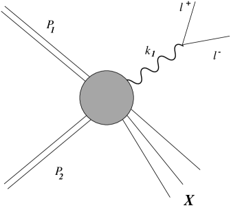
Figure 1: Drell-Yan process

Part of the calculations have been performed using FeynCalc [10], in particular the implementation of the Passarino-Veltman [11] recursion procedure for tensor integrals.The presentation of the phase space integration can be found in Appendix A, where we describe an extension to the polarized case of the previously known methods of integration used in the unpolarized case.

2 The Drell Yan Process

Deep Inelastic Scattering (DIS) has provided us with a wealth of information on the nucleon structure, however, there are limitations on the information obtainable from DIS experiments in the study of the spin properties of the hadrons. The first and most important limitation arises because gluons couple only to higher order. Also, distributions of transverse spin decouple. For a classification of the various light-cone operators of lowest and higher twist see [12], [13] and references therein. The Drell-Yan process is the natural territory to analyze $some$ of the issues connected with these important formal developments. For example, it has been observed (see for instance [13]) that the Drell-Yan production of charged lepton pairs is a case where transverse and longitudinal asymmetries are comparable. To leading order, the ratio between the transverse and the longitudinal asymmetries, $R=A_{TT}/A_{LL}$, is estimated to be of order one. This is due to the fact that the gluons don’t couple to transverse asymmetries and to order $\alpha_{s}$ only the quark-antiquark channel contributes. In other processes such as inclusive two-jet production ($p\,\,p\to j\,\,j+X$) or prompt photon production $\vec{p}\vec{p}\rightarrow\gamma+X$ the gluon channel is available also to leading order (in $A_{LL}$), thereby making $R$ small. Therefore, it is very important to see how these lowest order predictions are affected by radiative corrections.

Our work is concerned with a study of the differential cross section for the production of large transverse momentum lepton pairs, produced by the decay of a virtual photon of invariant mass $Q^{2}$. Since the lepton pair is required to have non-zero transverse momentum, $q_{T}$, the differential cross section starts at order $\alpha_{s}$. At lowest order (LO), one gluon (at least) is required to be in the final state. The calculation proceeds up to order $\alpha_{s}^{2}$ (denoted as NLO).

Figure 2: $\alpha_{s}$ order contributions

2.1 Previous Work

For the unpolarized case previous work on the process can be found in ref. [7] for the non-singlet sector. The total cross section, together with a calculation of the $K$ factor and a study of the small-$x$ limit has been studied by Van Neerven and collaborators (see [14] and refs. therein). In the polarized case, the order $\alpha_{s}$ radiative corrections have been originally investigated in [15] (total cross section). More recently work has been done to extend this calculation to the to the $x_{F}$-distribution in [16] to order $\alpha_{s}$. The resummation for the of the differential cross section at small $q_{T}$ of the lepton pair has been studied in the polarized case in [17]. The integration of our differential cross sections in dimensional regularization provides the bulk of the NNLO ($\alpha_{s}^{2}$) corrections to the total Drell-Yan cross section in the non-singlet sector. The remaining contributions, not included in this work, can be easily obtained by a simple extension of our work, since they amount to finite (in $\epsilon$) terms. However, as we are going to see, the structure of the helicity non-conserving contributions do not allow us to conclude that at parton level the total cross section is simply related to the unpolarized result by an overall helicity-dependent factor.

2.2 General Structure of the Differential Cross Section

We begin by examining the contribution to the production of virtual photons with invariant mass, $Q$, in hadron-hadron collisions,

$$H_{1}+H_{2}\to\gamma^{*}+X,$$ (1)

from the $2\to 3$ parton subprocess,

$$a+b\to\gamma^{*}+c+d,$$ (2)

like those shown in Figs. 4-6. Here $H_{1}$ and $H_{2}$ are incoming hadrons with 4-momenta, $P_{1}$ and $P_{2}$, respectively, and $q$ is the 4-momentum of the virtual photon, $\gamma^{*}$, as shown in Fig. 1. The 4-momenta of the incoming two parton $a$ and $b$ are labeled by $p_{1}$ and $p_{2}$ respectively, and the outgoing 4-momenta of partons $c$ and $d$ are labeled by $k_{2}$ and $k_{3}$. The virtual photon 4-momenta is given by $k_{1}=q$. Conservation of energy and momentum implies that

$$p_{1}+p_{2}=k_{1}+k_{2}+k_{3}.$$ (3)

The hadron-hadron process (1) is described in terms of the invariants,

$$S=(P_{1}+P_{2})^{2},\qquad T=(P_{1}-q)^{2},\qquad U=(P_{2}-q)^{2}.$$ (4)

In addition, it is convenient to define the scaled variables

$$x_{T}=2q_{T}/W\ {\rm and}\ \tau=Q^{2}/S,$$ (5)

where $W=\sqrt{S}$ is the hadron-hadron center-of-mass energy and $q_{T}$ is the transverse momentum of the virtual photon with invariant mass, $Q$. It is also useful to define the following two quantities,

$$\bar{x}_{1}={Q^{2}-U\over S}=\hbox{${1\over 2}$}e^{y}\sqrt{x_{T}^{2}+4\tau},\qquad\bar{x}_{2}={Q^{2}-T\over S}=\hbox{${1\over 2}$}e^{-y}\sqrt{x_{T}^{2}+4\tau},$$ (6)

where $y$ is the rapidity of the virtual photon. The $2\to 3$ parton subprocess (2) is described in terms of the invariants,

$$s=(p_{1}+p_{2})^{2},\qquad t=(p_{1}-q)^{2},\qquad u=(p_{2}-q)^{2},$$ (7)

and

$$s_{2}=s_{23}=(k_{2}+k_{3})^{2},$$ (8)

where momentum and energy conservation (3) implies

$$s+t+u=Q^{2}+s_{2}.$$ (9)

In QCD the hadronic cross section is related to the parton subprocess according to

$$d\sigma(H_{1}+H_{2}\to\gamma^{*}+X;W,q_{T},y)=$$ (10)

$$G_{H_{1}\to a}(x_{1},M^{2})dx_{1}G_{H_{2}\to b}(x_{2},M^{2})dx_{2}\left({d\hat{\sigma}\over dtdu}(ab\to\gamma^{*}cd;s,t,u)\right)dtdu,$$

where $G_{H_{1}\to a}(x_{1},M^{2})dx_{1}$ is the number of partons of flavor $a$ with momentum fraction, $x_{1}=p_{1}/P_{1}$, within hadron $H_{1}$ at the factorization scale $M$. Similarly, $G_{H_{2}\to b}(x_{2},M^{2})dx_{2}$ is the number of partons of flavor $b$ with momentum fraction, $x_{2}=p_{2}/P_{2}$, within hadron $H_{2}$ at the factorization scale $M$. In the remainder of this paper we will take the factorization scale to be $Q$ and evaluate the parton subprocesses at the same scale $Q$. Using (4) and (7) we see that

$$s = x_{1}x_{2}S,$$ (11)

$$(t-Q^{2}) = x_{1}(T-Q^{2})=-x_{1}\bar{x}_{2}S,$$ (12)

$$(u-Q^{2}) = x_{2}(U-Q^{2})=-x_{2}\bar{x}_{1}S,$$ (13)

which from (9) implies that

$$x_{1}x_{2}-x_{1}\bar{x}_{2}-x_{2}\bar{x}_{1}=\tau_{2}-\tau,$$ (14)

where $\bar{x}_{1}$ and $\bar{x}_{2}$ are defined in (6) and

$$\tau_{2}=s_{2}/S.$$ (15)

It is now easy to compute the Jacobian

$$dx_{2}dt={s\over 4(x_{1}-\bar{x}_{1})}\ dx_{T}^{2}dy,$$ (16)

which when inserted into (10) and integrating over $x_{1}$ and $s_{2}$ gives

$$S{d\sigma\over dq_{T}^{2}dy}(W,q_{T},y)=\int_{x_{1}^{min}}^{1}dx_{1}\int_{0}^{s_{2}^{max}}ds_{2}\ {1\over(x_{1}-\bar{x}_{1})}$$ (17)

$$\ G_{H_{1}\to a}(x_{1},Q^{2})G_{H_{2}\to b}(x_{2},Q^{2})\ s{d\hat{\sigma}\over dtdu}(ab\to\gamma^{*}cd;s,t,u),$$

where

$$x_{2}={x_{1}\bar{x}_{2}+\tau_{2}-\tau\over x_{1}-\bar{x}_{1}},$$ (18)

and

$$s_{2}^{max}=A=(\tau-\bar{x}_{1}+x_{1}(1-\bar{x}_{2}))S,\qquad x_{1}^{min}={\bar{x}_{1}-\tau\over 1-\bar{x}_{2}}.$$ (19)

The maximum value of $\tau_{2}$ arises when $x_{2}=1$ in (14), while the minimum value of $x_{1}$ occurs when $\tau_{2}=0$ and $x_{2}=1$.

For $2\to 2$ parton subprocesses such as the Born contribution in Fig. 2 one has

$$s{d\hat{\sigma}\over dtdu}(s,t,u)=\delta(s_{2})\ s{d\hat{\sigma}\over dt}(a+b\to\gamma^{*}+c;s,t),$$ (20)

which when inserted into (17) results in

$$S{d\sigma\over dq_{T}^{2}dy}(W,q_{T},y)=\int_{x_{1}^{min}}^{1}dx_{1}\ {1\over(x_{1}-\bar{x}_{1})}$$ (21)

$$\ G_{H_{1}\to a}(x_{1},Q^{2})G_{H_{2}\to b}(x_{2},Q^{2})\ s{d\hat{\sigma}\over dtdu}(ab\to\gamma^{*}c;s,t),$$

where in this case $s_{2}=0$ and $s+t+u=Q^{2}$. Finally, the Drell-Yan differential cross section for producing muon pair with transverse momentum $q_{T}$ and invariant mass, $Q$, at rapidity $y$ in the hadron-hadron collision,

$$H_{1}+H_{2}\to(\gamma^{*}\to\mu^{+}\mu^{-})+X,$$ (22)

at center-of-mass energy, $W$, is given by

$$S{d\sigma\over dQ^{2}dq_{T}^{2}dy}(H_{1}H_{2}\to\mu^{+}\mu^{-}+X;W,q_{T},y)=$$ (23)

$$\left({\alpha\over 3\pi Q^{2}}\right)S{d\sigma\over dq_{T}^{2}dy}(H_{1}H_{2}\to\gamma^{*}+X;W,q_{T},y),$$

where $\alpha$ is the electromagnetic fine structure constant and where the virtual photon differential cross section is given by (17) or (21). In the remainder of this paper we will concentrate on the virtual photon differential cross section.

2.3 The Non-Singlet Cross Section

We define the non-singlet to be the difference of the antihadron-hadron and the hadron-hadron differential cross sections as follows:

$$S{d\sigma_{NS}\over dq_{T}^{2}dy}(H+H_{2}\to\gamma^{*}+X)=$$ (24)

$$S{d\sigma\over dq_{T}^{2}dy}(\bar{H}+H_{2}\to\gamma^{*}+X)-S{d\sigma\over dq_{T}^{2}dy}(H+H_{2}\to\gamma^{*}+X).$$

It is easy to see that

$$S{d\sigma_{NS}\over dq_{T}^{2}dy}(W,q_{T},y)=\sum_{f,f^{\prime}}\int_{x_{1}^{min}}^{1}dx_{1}\int_{0}^{s_{2}^{max}}ds_{2}\ {1\over(x_{1}-\bar{x}_{1})}$$ (25)

$$\ G^{NS}_{H\to q_{f}}(x_{1},Q^{2})G^{NS}_{H\to q_{f^{\prime}}}(x_{2},Q^{2})\ s{d{\hat{\sigma}}_{NS}\over dtdu}(s,t,u),$$

where the non-singlet parton-parton differential cross section is given by

$$s{d{\hat{\sigma}}_{NS}\over dtdu}=s{d{\hat{\sigma}}\over dtdu}(\bar{q}_{f}q_{f^{\prime}}\to\gamma^{*}+X)-s{d{\hat{\sigma}}\over dtdu}(q_{f}q_{f^{\prime}}\to\gamma^{*}+X),$$ (26)

and the non-singlet structure function is defined according to

$$G^{NS}_{H\to q}=G_{H\to q}-G_{H\to\bar{q}}.$$ (27)

The sum in (25) is over the quark flavors $f$ and $f^{\prime}$. As we will see this sum turns out to be diagonal in flavor space so that one needs only to sum over $f=f^{\prime}$.

We will organize the Feynman diagrams in the same way as was done in [7]. At order $\alpha_{s}$ the Born term comes only from the square of the two amplitudes in Fig. 2, which we write schematically as

$$d{\hat{\sigma}}_{B}\sim|L_{1}+L_{2}|^{2}.$$ (28)

The Born term contributes only to the diagonal $\bar{q}_{f}q_{f}$ part of the non-singlet differential cross section in (25) since it is non zero only when $f=f^{\prime}$.

The order $\alpha_{s}^{2}$ contributions are separated into the real and the virtual diagrams. The virtual term, $d{\hat{\sigma}}^{virtual}$ comes from the interference between the amplitudes $L_{1}$ and $L_{2}$ and the eleven amplitudes shown in Fig. 6,

$$d{\hat{\sigma}}^{virtual}\sim 2Re\left((L_{1}+L_{2})\sum_{i=1}^{11}V_{i}^{*}\right),$$ (29)

which again contributes only to the diagonal $\bar{q}_{f}q_{f}$ part of the non-singlet differential cross section in (25).

The other real diagonal $\bar{q}_{f}q_{f}$ diagrams are

$$d{\hat{\sigma}}^{real}_{\bar{q}_{f}q_{f}}\sim|\sum_{i=1}^{8}F_{i}|^{2}+|\sum_{i=1}^{8}G_{i}|^{2},$$ (30)

where the amplitudes $F_{i}$ are shown in Fig. 3 and the amplitudes $G_{i}$ are shown in Fig. 4 with $f=f^{\prime}$. The absolute square of the $F_{i}$ amplitudes can be written as follows:

$$|\sum_{i=1}^{8}F_{i}|^{2}=$$ (31)

$$|F_{1}+F_{2}|^{2}+|F_{3}+F_{4}|^{2}+2Re\left(\sum_{i=1}^{4}F_{i}\sum_{i=5}^{8}F^{*}_{i}\right)+|\sum_{i=5}^{8}F_{i}|^{2},$$

where we have used the fact that

$$Re\left((F_{1}+F_{2})(F_{3}+F_{4})^{*}\right)=0.$$ (32)

Thus the diagonal real $\bar{q}_{f}q_{f}$ contributions are,

$$d{\hat{\sigma}}^{real}_{\bar{q}_{f}q_{f}}=d{\hat{\sigma}}_{1}+d{\hat{\sigma}}_{2}+d{\hat{\sigma}}_{3}+d{\hat{\sigma}}_{F},$$ (33)

where

$$d{\hat{\sigma}}_{1} \sim |F_{1}+F_{2}|^{2}+|\sum_{i=1}^{8}G_{i}|^{2},$$ (34)

$$d{\hat{\sigma}}_{2} \sim |F_{3}+F_{4}|^{2},$$ (35)

$$d{\hat{\sigma}}_{3} \sim 2Re\left(\sum_{i=1}^{4}F_{i}\sum_{i=5}^{8}F^{*}_{i}\right),$$ (36)

$$d{\hat{\sigma}}_{F} \sim |\sum_{i=5}^{8}F_{i}|^{2}.$$ (37)

The real diagonal $q_{f}q_{f}$ diagrams are

$$d{\hat{\sigma}}^{real}_{q_{f}q_{f}}\sim|\sum_{i=1}^{4}H_{i}-\sum_{i=4}^{8}H_{i}|^{2},$$ (38)

where the amplitudes $H_{i}$ are shown in Fig. 5 and the relative minus sign between the direct and exchange diagrams is due to Fermi statistics since $f=f^{\prime}$. The absolute square of the $H_{i}$ amplitudes can be written as follows:

$$|\sum_{i=1}^{4}H_{i}-\sum_{i=4}^{8}H_{i}|^{2}=$$ (39)

$$|\sum_{i=1}^{4}H_{i}|^{2}+|\sum_{i=4}^{8}H_{i}|^{2}-2Re\left(\sum_{i=1}^{4}H_{i}\sum_{i=4}^{8}H_{i}^{*}\right).$$

Thus the diagonal real $q_{f}q_{f}$ contributions are,

$$d{\hat{\sigma}}^{real}_{q_{f}q_{f}}=d{\hat{\sigma}}_{H}+d{\hat{\sigma}}_{4},$$ (40)

where

$$d{\hat{\sigma}}_{H} \sim |\sum_{i=1}^{4}H_{i}|^{2}+|\sum_{i=4}^{8}H_{i}|^{2},$$ (41)

$$d{\hat{\sigma}}_{4} \sim -2Re\left(\sum_{i=1}^{4}H_{i}\sum_{i=4}^{8}H_{i}^{*}\right).$$ (42)

The diagonal ($f=f^{\prime}$) real part of the non-singlet cross section in (26) is given by subtracting (40) from (33) as follows:

$$d{\hat{\sigma}}^{real}_{NS}=d{\hat{\sigma}}_{1}+d{\hat{\sigma}}_{2}+d{\hat{\sigma}}_{3}-d{\hat{\sigma}}_{4},$$ (43)

where we have used the fact that $d{\hat{\sigma}}_{F}=d{\hat{\sigma}}_{H}$ which arises due to

$$\int_{PS_{3}}|\sum_{i=5}^{8}F_{i}|^{2}=\hbox{${1\over 2}$}\int_{PS_{3}}|\sum_{i=1}^{4}H_{i}|^{2}+\hbox{${1\over 2}$}\int_{PS_{3}}|\sum_{i=4}^{8}H_{i}|^{2}.$$ (44)

When integrating over the two identical particles $k_{3}$ and $k_{4}$ over the phase space $PS_{3}$ in (141) an extra statistical factor of $1/2$ must be inserted so as not to double count. Thus, the diagonal ($f=f^{\prime}$) part of the complete non-singlet cross section in (26) (real plus virtual) is given by

$$d{\hat{\sigma}}_{NS}=d{\tilde{\sigma}}_{1}+d{\hat{\sigma}}_{2}+d{\hat{\sigma}}_{3}-d{\hat{\sigma}}_{4},$$ (45)

where

$$d{\tilde{\sigma}}_{1}=d{\hat{\sigma}}^{fact}_{1}+d{\hat{\sigma}}^{virtual},$$ (46)

and where $d{\hat{\sigma}}^{fact}_{1}$ is the “factorized” cross section given by

$$d{\hat{\sigma}}^{fact}_{1}=d{\hat{\sigma}}_{1}+d{\hat{\sigma}}^{counter}_{1}.$$ (47)

It is necessary to add a “counterterm” cross section $d{\hat{\sigma}}^{counter}_{1}$ to $d{\hat{\sigma}}_{1}$ to cancel the initial state collinear singularities.

The off-diagonal real $\bar{q}_{f}q_{f^{\prime}}$ diagrams are

$$d{\hat{\sigma}}^{real}_{\bar{q}_{f}q_{f^{\prime}}}\sim|\sum_{i=1}^{4}F_{i}|^{2},$$ (48)

where the amplitudes $F_{i}$ are shown in Fig. 3 and where $f\neq f^{\prime}$. Similarly, the off-diagonal real diagonal $q_{f}q_{f^{\prime}}$ diagrams are

$$d{\hat{\sigma}}^{real}_{q_{f}q_{f^{\prime}}}\sim|\sum_{i=1}^{4}H_{i}|^{2},$$ (49)

where the amplitudes $H_{i}$ are shown in Fig. 5. In this case,

$$|\sum_{i=1}^{4}F_{i}|^{2}=|\sum_{i=1}^{4}H_{i}|^{2},$$ (50)

so that these two contributions cancel when forming the non-singlet cross section in (26). Thus to order $\alpha_{s}^{2}$ (25) becomes

$$S{d\sigma_{NS}\over dq_{T}^{2}dy}(W,q_{T},y)=\sum_{f}\int_{x_{1}^{min}}^{1}dx_{1}\int_{0}^{s_{2}^{max}}ds_{2}\ {1\over(x_{1}-\bar{x}_{1})}$$ (51)

$$\ G^{NS}_{H\to q_{f}}(x_{1},Q^{2})G^{NS}_{H\to q_{f}}(x_{2},Q^{2})\ s{d{\hat{\sigma}}_{NS}\over dtdu}(s,t,u),$$

where the sum is now only over the quark flavor $f$ and where

$$s{d{\hat{\sigma}}_{NS}\over dtdu}=s{d{\hat{\sigma}}_{B}\over dtdu}+s{d{\tilde{\sigma}}_{1}\over dtdu}+s{d{\hat{\sigma}}_{2}\over dtdu}+s{d{\hat{\sigma}}_{3}\over dtdu}-s{d{\hat{\sigma}}_{4}\over dtdu}.$$ (52)

2.4 The Helicity Dependence of the Born Term

The lowest order (non-singlet) contributions to the large transverse momentum production of virtual photons (see Fig. 2) with invariant mass $q^{2}=Q^{2}$ arise from the two, $q+\bar{q}\to\gamma^{*}+g$, “Born” amplitudes $L_{1}$ and $L_{2}$. We refer to these two diagrams as the direct and the exchange (or crossed) amplitudes, respectively. The absolute square of the sum of these amplitudes form the Born differential cross section in (28). In Fig. 2 we have also generically illustrated the expansion of the amplitude which appears in $d\sigma/d\,Q^{2}$ up to order $\alpha_{s}$. Notice that the quark form factor contributions in Fig.2 (and the related $O(\alpha_{s}^{2})$ corrections, not included in the picture) do not appear in the study of the cross section, $d\sigma/dq^{2}_{T}d\,y$, for transverse momentum, $q_{T}$, greater than zero. The two-loop $O(\alpha_{s}^{2})$ corrections to the quark form factor can be added in the study of the total cross section, $d\sigma/d\,Q^{2}$, by interfering the 2-loop on-shell quark form factor of ref. [18] with the lowest order $q\bar{q}\gamma^{*}$ annihilation channel and by using helicity projectors for the initial quark states.

We calculate the spin dependence of the cross section by using the helicity projectors, $P_{\pm}={1\over 2}(1\pm\gamma_{5})$, which project out the helicity states of an initial state quark and antiquark, respectively, as follows:

$$u(p_{1},h_{1})={1\over 2}(1+h_{1}\gamma_{5})u(p_{1}),\qquad\bar{v}(p_{2},h_{2})={1\over 2}\bar{v}(p_{2})(1+h_{2}\gamma_{5}),$$ (53)

where $h_{1}=\pm 1=2\lambda_{1}$ corresponds to quark helicity $\lambda_{1}=\pm{1\over 2}$, and $h_{2}=\pm 1=2\lambda_{2}$ corresponds to antiquark helicity $\lambda_{2}=\pm{1\over 2}$.

The squares of the direct amplitude $L_{1}$ and exchange amplitude $L_{2}$ in Fig. 2 in $N=4-2\epsilon$ dimensions are given by

$$M_{dd}(h_{1},h_{2})=e_{f}^{2}g^{2}g_{s}^{2}{C_{F}\over N_{c}}{2u\over t}\left((1-\epsilon)^{2}-h_{1}h_{2}(1+\epsilon)^{2}\right),$$

$$M_{cc}(h_{1},h_{2})=e_{f}^{2}g^{2}g_{s}^{2}{C_{F}\over N_{c}}{2t\over u}\left((1-\epsilon)^{2}-h_{1}h_{2}(1+\epsilon)^{2}\right).$$ (54)

where $\alpha=g^{2}/4\pi$ is the fine structure constant, and $e_{f}$ the charge of the quark. The quantity $C_{F}/N_{c}$ is the color factor, and $\alpha_{s}=g_{s}^{2}/4\pi$ is the QCD strong coupling constant. We pause here to note that in our NLO calculation $\alpha_{s}\to\alpha_{s}(\mu^{2})$ is the running coupling constant renormalized at the scale $\mu^{2}$ in the $\overline{MS}$ scheme satisfying the renormalization group equation

$$\mu^{2}\frac{d\alpha_{s}}{d\mu^{2}}=-\alpha_{s}\left[\beta_{0}\frac{\alpha_{s}}{4\pi}+\beta_{1}\left(\frac{\alpha_{s}}{4\pi}\right)^{2}+O(\alpha_{s}^{3})\right]$$ (55)

with

$$\beta_{0} = \frac{11N_{C}}{3}-\frac{2N_{F}}{3}$$

$$\beta_{1} = \frac{34N_{C}^{2}}{3}-\frac{10N_{C}N_{F}}{3}-2C_{F}N_{F}$$ (56)

and with $N_{F}$ the number of active quark flavors. The interference term is more complicated and is given by,

$$2M_{dc}(h_{1},h_{2})=$$

$$e_{f}^{2}g^{2}g_{s}^{2}{C_{F}\over N_{c}}{4\over tu}\left[(1-\epsilon)(Q^{2}s-\epsilon tu)\right.\left.-h_{1}h_{2}(1+\epsilon)(Q^{2}s+\epsilon tu)-2h_{1}h_{2}\epsilon tu\right].$$ (57)

The sum of the two Born amplitudes squared is

$$|M_{B}(h_{1},h_{2})|^{2}=|M_{B}(h)|^{2}=M_{dd}(h)+2M_{dc}(h)+M_{cc}(h)$$

$$=e_{f}^{2}g^{2}g_{s}^{2}{C_{F}\over N_{c}}{2\over tu}\left[(1-\epsilon)\left(2Q^{2}s+(1-\epsilon)(t^{2}+u^{2})-2\epsilon tu\right)\right.$$

$$\left.-h(1+\epsilon)\left(2Q^{2}s+(1+\epsilon)(t^{2}+u^{2})+2\epsilon tu\right)-4h\epsilon tu\right],$$ (58)

and depends only on the product $h=h_{1}h_{2}$.

To any order in perturbation theory we can write,

$$|M(h_{1},h_{2})|^{2}=|M(h)|^{2}=(1-h)|\overline{M}|^{2}+h|M_{++}|^{2}=|\overline{M}|^{2}+h\Delta|M|^{2},$$ (59)

where $h=h_{1}h_{2}=4\lambda_{1}\lambda_{2}$ and where

$$|\overline{M}|^{2}={1\over 4}|\sum_{h_{1},h_{2}}M(h_{1},h_{2})|^{2}={1\over 4}\sum_{h_{1},h_{2}}|M(h_{1},h_{2})|^{2},$$ (60)

is the spin averaged (unpolarized) amplitude squared. Furthermore,

$$|M_{--}|^{2}=|M_{++}|^{2}\ {\rm and}\ |M_{-+}|^{2}=|M_{+-}|^{2},$$ (61)

so that

$$|\overline{M}|^{2}={1\over 2}\left(|M_{++}|^{2}+|M_{+-}|^{2}\right).$$ (62)

The spin asymmetry, $\Delta|M|^{2}$, is defined according to

$$\Delta|M|^{2}={1\over 2}\left(|M_{++}|^{2}-|M_{+-}|^{2}\right)=|M_{++}|^{2}-|\overline{M}|^{2}.$$ (63)

The spin averaged (unpolarized) amplitude squared is determined from $|M(h)|^{2}$ by setting $h=0$ with $\Delta|M|^{2}$ the coefficient of $h$. For the Born term, this results in

$$|\overline{M}|^{2}=e_{f}^{2}g^{2}g_{s}^{2}{C_{F}\over N_{c}}{2\over tu}\left[(1-\epsilon)\left(2Q^{2}s+(1-\epsilon)(t^{2}+u^{2})-2\epsilon tu\right)\right],$$ (64)

and

$$\Delta|M|^{2}=-e_{f}^{2}g^{2}g_{s}^{2}{C_{F}\over N_{c}}{2\over tu}\left[(1+\epsilon)\left(2Q^{2}s+(1+\epsilon)(t^{2}+u^{2})+2\epsilon tu\right)+4\epsilon tu\right].$$ (65)

Adding these two terms yields

$$|M_{++}|^{2}=-e_{f}^{2}g^{2}g_{s}^{2}{C_{F}\over N_{c}}{8\epsilon\over tu}\left[Q^{2}s+(t+u)^{2}\right],$$ (66)

which is proportional to $\epsilon$ and vanishes in the limit $\epsilon\rightarrow 0$. Since at the Born level there are no ${1\over\epsilon}$ singularities that might combine with this term to yield a finite contribution, in the limit $\epsilon\rightarrow 0$,

$$|M_{++}|^{2}=0\ {\rm and}\ \Delta|M|^{2}=-|\overline{M}|^{2}.$$ (67)

For the $q+\bar{q}\to\gamma^{*}+g$ subprocess the condition that $|M_{++}|^{2}=0$ means that the quark helicity is maintained (does not flip) in the collision. The incoming quark line with helicity $\pm{1\over 2}$ turns around and becomes an incoming antiquark with helicity $\mp{1\over 2}$. We refer to this as “helicity conservation”. We see that at the Born level helicity is conserved in the limit $\epsilon\rightarrow 0$.

In $N=4-2\epsilon$ dimensions the differential cross section is related to the $2\to 2$ invariant amplitude according to

$$s{d\hat{\sigma}\over dt}(s,t,h)={1\over 16\pi s}\left({4\pi s\over tu}\right)^{\epsilon}{1\over\Gamma(1-\epsilon)}|M(h)|^{2},$$ (68)

which can be written as

$$s{d\hat{\sigma}\over dt}(s,t,h)=(1-h)\ s{d\hat{\sigma}^{\Sigma}\over dt}(s,t)+h\ s{d\hat{\sigma}_{++}\over dt}(s,t),$$ (69)

or as

$$s{d\hat{\sigma}\over dt}(s,t,h)=s{d\hat{\sigma}^{\Sigma}\over dt}(s,t)+h\ s{d\hat{\sigma}_{LL}\over dt}(s,t),$$ (70)

where $sd\hat{\sigma}^{\Sigma}/dt$ is the unpolarized cross section

$$s{d\hat{\sigma}^{\Sigma}\over dt}={1\over 2}\left(s{d\hat{\sigma}_{++}\over dt}+s{d\hat{\sigma}_{+-}\over dt}\right).$$ (71)

and

$$s{d\hat{\sigma}_{LL}\over dt}={1\over 2}\left(s{d\hat{\sigma}_{++}\over dt}-s{d\hat{\sigma}_{+-}\over dt}\right).$$ (72)

At the Born level we have,

$$s{d\hat{\sigma}_{B}^{\Sigma}\over dt}(s,t)=e_{f}^{2}K_{2}{\alpha_{s}\over s}T_{B}(Q^{2},u,t),$$

$$s{d\hat{\sigma}_{B}^{++}\over dt}(s,t)=-e_{f}^{2}K_{2}{\alpha_{s}\over s}\epsilon A_{B}(Q^{2},u,t),$$ (73)

where

$$T_{B}(Q^{2},u,t)={2\over tu}\left[(1-\epsilon)\left(2Q^{2}s+(1-\epsilon)(t^{2}+u^{2})-2\epsilon tu\right)\right]$$

$$=2(1-\epsilon)\left[(1-\epsilon)\left({u\over t}+{t\over u}\right)+{2Q^{2}(Q^{2}-u-t)\over ut}-2\epsilon\right],$$ (74)

and

$$A_{B}(Q^{2},u,t)={8\over tu}\left[Q^{2}s+(t+u)^{2}\right],$$ (75)

where $K_{2}$ is defined by

$$K_{2}=\pi\alpha{C_{F}\over N_{c}}{1\over\Gamma(1-\epsilon)}\left({4\pi\mu^{2}\over Q^{2}}\right)^{\epsilon}\left({sQ^{2}\over tu}\right)^{\epsilon},$$ (76)

where we have rescaled, $\alpha_{s}\to\alpha_{s}(\mu^{2})^{\epsilon}$, so that it remains dimensionless in $N=4-2\epsilon$ dimensions. At this order of perturbation theory, we have

$$s{d\hat{\sigma}_{B}\over dt}(s,t,h)=e_{f}^{2}K_{2}{\alpha_{s}\over s}\left[(1-h)T_{B}(Q^{2},u,t)-h\epsilon A_{B}(Q^{2},u,t)\right].$$ (77)

As we saw earlier, in the limit $\epsilon\to 0$ helicity is conserved so that

$$s{d\hat{\sigma}_{B}\over dt}(s,t,h)=(1-h)s{d\hat{\sigma}_{B}^{\Sigma}\over dt}(s,t),$$ (78)

which implies that

$$s{d\hat{\sigma}_{B}^{++}\over dt}(s,t)=0\ {\rm and}\ s{d\hat{\sigma}_{B}^{LL}\over dt}(s,t)=-s{d\hat{\sigma}_{B}^{\Sigma}\over dt}(s,t),$$ (79)

so that to leading order,

$$\hat{A}_{LL}={d\hat{\sigma}_{LL}\over dt}\bigg{/}{d\hat{\sigma}^{\Sigma}\over dt}=-1.$$ (80)

To connect with the notation of ref. [7], we note that

$$K_{2}T_{B}(Q^{2},u,t)=KT_{0}(Q^{2},u,t),$$ (81)

where $K$ and $T_{0}$ are define in ref. [7] as

$$K=2\pi\alpha{C_{F}\over N_{c}}{(1-\epsilon)\over\Gamma(1-\epsilon)}\left({4\pi\mu^{2}\over Q^{2}}\right)^{\epsilon}\left({sQ^{2}\over tu}\right)^{\epsilon},$$ (82)

and

$$T_{0}(Q^{2},u,t)=\left[(1-\epsilon)\left({u\over t}+{t\over u}\right)+{2Q^{2}(Q^{2}-u-t)\over ut}-2\epsilon\right].$$ (83)

2.5 General Structure of the Helicity Dependent Cross Section

To order $\alpha_{s}^{2}$ the non-singlet helicity dependent Drell Yan cross section can be written according to (51). Namely,

$$S{d\sigma_{NS}\over dq_{T}^{2}dy}(W,q_{T},y,\Lambda_{1},\Lambda_{2})=\sum_{f}\sum_{\lambda_{1},\lambda_{2}}\int_{x_{1}^{min}}^{1}dx_{1}\int_{0}^{s_{2}^{max}}ds_{2}\ {1\over(x_{1}-\bar{x}_{1})}$$ (84)

$$\ G^{NS}_{H[\Lambda_{1}]\to q_{f}[\lambda_{1}]}(x_{1},Q^{2})G^{NS}_{H[\Lambda_{2}]\to q_{f}[\lambda_{2}]}(x_{2},Q^{2})\ s{d{\hat{\sigma}}_{NS}\over dtdu}(s,t,u,h),$$

where $\Lambda_{1}$ and $\Lambda_{2}$ are the helicities of the initial two hadrons, respectively, and $h=4\lambda_{1}\lambda_{2}$ and where the sum is now over the quark flavor $f$ and the parton helicities $\lambda_{1}$ and $\lambda_{2}$. The non-singlet polarized structure functions are given by

$$G^{NS}_{H[\Lambda]\to q_{f}[\lambda]}=G_{H[\Lambda]\to q_{f}[\lambda]}-G_{H[\Lambda]\to\bar{q}_{f}[\lambda]}.$$ (85)

The parton-parton non-singlet differential can be written as a function of $h$ as follows:

$$s{d{\hat{\sigma}}_{NS}\over dtdu}(s,t,u,h)=$$ (86)

$$s{d{\hat{\sigma}}_{B}\over dtdu}(h)+s{d{\tilde{\sigma}}_{1}\over dtdu}(h)+s{d{\hat{\sigma}}_{2}\over dtdu}(h)+s{d{\hat{\sigma}}_{3}\over dtdu}(h)-s{d{\hat{\sigma}}_{4}\over dtdu}(h).$$

From (78) we see helicity is conserved for the Born term so that

$$s{d\hat{\sigma}_{B}\over dtdu}(s,t,u,h)=(1-h)\delta(s_{2})\ s{d\hat{\sigma}_{B}^{\Sigma}\over dt}(s,t),$$ (87)

where $d\hat{\sigma}_{B}^{\Sigma}$ is the unpolarized cross section in (73). Helicity is also conserved for $d\hat{\sigma}_{2}$ defined in (35) and for $d\hat{\sigma}_{3}$ defined in (36) so that

$$s{d\hat{\sigma}_{2}\over dtdu}(s,t,u,h)=(1-h)\ s{d\hat{\sigma}_{2}^{\Sigma}\over dtdu}(s,t,u),$$ (88)

and

$$s{d\hat{\sigma}_{3}\over dtdu}(s,t,u,h)=(1-h)\ s{d\hat{\sigma}_{3}^{\Sigma}\over dtdu}(s,t,u).$$ (89)

The Born term and these two cross sections have the property that $d\hat{\sigma}_{(}++)=0$ as expected from helicity conservation. The term $d\hat{\sigma}_{4}$ defined in (42) is different. Here helicity conservation implies that $d\hat{\sigma}_{(}+-)=0$ and we have

$$s{d\hat{\sigma}_{4}\over dtdu}(s,t,u,h)=(1+h)\ s{d\hat{\sigma}_{4}^{\Sigma}\over dtdu}(s,t,u).$$ (90)

The term $d\tilde{\sigma}_{1}$ is complicated and whether helicity is conserved or not depends on how one does the factorization in (47). We write the helicity structure as follows:

$$s{d\tilde{\sigma}_{1}\over dtdu}(s,t,u,h)=(1-h)\ s{d\tilde{\sigma}_{1}^{\Sigma}\over dtdu}(s,t,u)+h\ s{d\hat{\sigma}^{hat}_{0}\over dtdu}(s,t,u),$$ (91)

where $d\hat{\sigma}^{hat}_{0}$ is a regularization scheme dependent helicity non-conserving piece and $d\tilde{\sigma}_{1}^{\Sigma}$ is the unpolarized spin-averaged cross section.

To order $\alpha_{s}^{2}$ the non-singlet parton level spin asymmetry defined in (72) becomes

$$s{d{\hat{\sigma}}^{LL}_{NS}\over dtdu}(s,t,u)=-s{d{\hat{\sigma}}^{\Sigma}_{NS}\over dtdu}+s{d{\hat{\sigma}}^{hat}_{0}\over dtdu}-2s{d{\hat{\sigma}}^{\Sigma}_{4}\over dtdu},$$ (92)

where $d{\hat{\sigma}}^{\Sigma}_{NS}$ is the non-singlet unpolarized spin averaged cross section given by

$$s{d{\hat{\sigma}}^{\Sigma}_{NS}\over dtdu}(s,t,u)=s{d{\hat{\sigma}}_{B}^{\Sigma}\over dtdu}+s{d{\tilde{\sigma}}_{1}^{\Sigma}\over dtdu}+s{d{\hat{\sigma}}_{2}^{\Sigma}\over dtdu}+s{d{\hat{\sigma}}_{3}^{\Sigma}\over dtdu}-s{d{\hat{\sigma}}_{4}^{\Sigma}\over dtdu}.$$ (93)

At the parton level it is no longer true that $\hat{A}_{LL}=-1$ as was the case for the Born term in (80).

3 Virtual Diagram Contributions

The list of the diagrams with virtual corrections contributing to the non-singlet sector is defined in (29) and shown in Fig. 6. We have omitted all the self-energy insertions of quarks and gluons and the ghost contributions.

Our calculations are performed in the $\overline{MS}$ scheme using dimensional regularization to regulate both the ultraviolet and the infrared singularities. We remove the ultraviolet singularities in the relevant subdiagrams by off shell regularization. Then by sending on shell the initial state quarks and the final state gluon, we encounter singularities in the form of double poles and single poles in $\epsilon=2-n/2$. The renormalization of the diagrams is enforced in such a way to get straightforwardly final results free of UV singularities by symbolic manipulation. We briefly comment here on how this is achieved in our case, although a more detailed discussion of the method will be presented elsewhere. As a first step, we start with the Passarino-Veltman reduction of the tensor contributions and generate the expression of the invariant amplitudes of the reduction. In our case only one external line (the photon ) is massive. The calculation is ambiguous because of the presence of massless partons and, in principle, one has to be particularly careful to differentiate between the UV and the IR origin of all the singularities, which in our approach happen to be identified ($\epsilon_{UV}=\epsilon_{IR}$ in Dimensional Regularization). Therefore, the expressions of the invariant amplitudes in the Passarino Veltman reduction are, at this stage, unrenormalized.

At the second step, we renormalize the scalar diagrams which appear in the result by removing the UV poles, (since these are removed by coupling constant renormalization) and then switch $\epsilon\to-\epsilon$ in the final result. This allows us to at this stage interpret the left over singularities as IR singularities. Even at this stage the procedure is not complete. One needs a prescription to handle the massless tadpoles (self energies at zero momentum) in a consistent way. The Passarino Veltman procedure in the massless case, in fact, suffers from ambiguities of this type, since massless tadpoles are intrinsically ill-defined (being scaleless). In dimensional regularization they are usually set to vanish. However, since we have identified UV and IR singularities in our algorithm, this last step is also ambiguous.

At the third step we impose two prescriptions which allow us to handle consistently way all the tadpoles and all the massive self energy contributions. These include :

1. isolated tadpoles (B(0)) and “linear” tadpoles (or $\epsilon B(0)$ terms).

2. massive self energy contributions ($B(q^{2})$ and $\epsilon B(q^{2})$).

In (2) we implement off-shell renormalization, while in (1) we reinterpret all the scaleless contributions as the massless limit of the off-shell ones. After step 3, we obtain the correct renormalized expressions of all the Passarino Veltman coefficients for all the one-loop amplitude. The method works at one loop for any $n$-point function and is extremely convenient in practical applications since it allows us to forget about the nature of the singularities after $IR/UV$ identification. The symbolic implementation of the method is also quite straightforward and will be illustrated elsewhere [20].

The one-loop order result for the cross section for the process $q+\bar{q}\rightarrow\gamma^{*}+g$ is given by

$$s{d\hat{\sigma}^{\rm virtual}\over dtdu}(s,t,u,h)=$$

$$e^{2}_{f}K_{2}\frac{\alpha_{s}}{s}\delta(s+t+u-Q^{2})\left\{\left((1-h)T_{B}-h\epsilon A_{B}\right)\left[1-\frac{\alpha_{s}}{2\pi}\frac{\Gamma(1-\epsilon)}{\Gamma(1-2\epsilon)}\left(\frac{4\pi\mu^{2}}{Q^{2}}\right)^{\epsilon}\right.\right.$$

$$\left.\times\left(\frac{2C_{F}+N_{C}}{\epsilon^{2}}+\frac{1}{\epsilon}\left(3C_{F}-2C_{F}\ln\frac{s}{Q^{2}}+\frac{11}{6}N_{C}+N_{C}\ln\frac{sQ^{2}}{ut}-\frac{1}{3}N_{F}\right)\right)\right]$$

$$+\frac{\alpha}{2\pi}(1-h)\left[\pi^{2}(4C_{F}+N_{C})\frac{2Q^{2}s+t^{2}+u^{2}}{3tu}-2(2C_{F}-N_{C})\frac{Q^{2}(t^{2}+u^{2})}{tu(t+u)}\right.$$

$$-2C_{F}\left(\frac{8(2Q^{2}s+t^{2}+u^{2})}{tu}-\frac{Q^{4}s(t+u)}{tu(Q^{2}-u)(Q^{2}-t)}-\frac{t^{2}+u^{2}}{(Q^{2}-u)(Q^{2}-t)}\right)$$

$$-2\left(Li_{2}\left(\frac{t}{t-Q^{2}}\right)+\frac{1}{2}\ln^{2}\left(1-\frac{Q^{2}}{t}\right)\right)\left(N_{C}\frac{2s+t}{u}+2C_{F}\frac{s^{2}+(s+u)^{2}}{tu}\right)$$

$$-2\left(Li_{2}\left(\frac{u}{u-Q^{2}}\right)+\frac{1}{2}\ln^{2}\left(1-\frac{Q^{2}}{u}\right)\right)\left(N_{C}\frac{2s+u}{t}+2C_{F}\frac{s^{2}+(s+t)^{2}}{tu}\right)$$

$$+2(2C_{F}-N_{C})\left(Li_{2}\left(-\frac{t+u}{s}\right)\frac{2Q^{2}s+u^{2}+t^{2}+2s^{2}}{tu}\right.$$

$$+\left(2\ln\left(\frac{s}{Q^{2}}\right)\frac{Q^{4}-(t+u)^{2}}{(t+u)^{2}}+\ln^{2}\left(\frac{s}{Q^{2}}\right)\frac{s^{2}}{tu}\right)$$

$$-\left(\ln\left(\frac{|t|}{Q^{2}}\right)\ln\left(\frac{s}{Q^{2}}\right)-\frac{1}{2}\ln^{2}\left(\frac{|t|}{Q^{2}}\right)\right)\frac{s^{2}+(s+u)^{2}}{tu}$$

$$\left.-\left(\ln\left(\frac{s}{Q^{2}}\right)\ln\left(\frac{|u|}{Q^{2}}\right)-\frac{1}{2}\ln^{2}\left(\frac{|u|}{Q^{2}}\right)\right)\frac{s^{2}+(s+t)^{2}}{tu}\right)$$

$$+2\ln\left(\frac{|u|}{Q^{2}}\right)\left(C_{F}\frac{4Q^{2}s-2su+tu}{(Q^{2}-u)^{2}}+N_{C}\frac{u}{Q^{2}-u}\right)$$

$$+2\ln\left(\frac{|t|}{Q^{2}}\right)\left(C_{F}\frac{4Q^{2}s-2st+tu}{(Q^{2}-t)^{2}}+N_{C}\frac{t}{Q^{2}-t}\right)$$

$$\left.\left.-2\ln\left(\frac{|t|}{Q^{2}}\right)\ln\left(\frac{|u|}{Q^{2}}\right)N_{C}\frac{2Q^{2}s+t^{2}+u^{2}}{tu}\right]\right\},$$ (94)

where $h=h_{1}h_{2}=4\lambda_{1}\lambda_{2}$. This result agrees with the (unpolarized) spin-averaged ($h\to 0$) result given in [7], although its structure is more simplified since we have performed some additional manipulations on the finite contributions. Therefore, we confirm the result of [7], which had been used before by other authors [21, 22], but never checked before. The quantities $T_{B}$ and $A_{B}$ appear in at the Born level and are given by equations (74) and (75), respectively. Notice that the double poles and single pole structure (in the $h\to 0$ limit) automatically reproduces the singularities of the virtual contributions of ref. [7]. In particular, the double poles in $\epsilon$ correctly multiply the two-to-two Born contribution $T_{B}$, which is the Born level unpolarized result. The presence of the $h\epsilon A_{B}$ term in (94) implies that in the t’Hooft-Veltman [8, 19] scheme the virtual corrections by themselves do not conserve helicity (i.e. they do not satisfy the equation (78)). In particular, the finite part of $d\hat{\sigma}_{++}/dt$ in the limit $\epsilon\to 0$ for the virtual corrections is given by

$$s{d\hat{\sigma}_{++}^{\rm virtual}\over dt}(s,t)=$$

$$-e^{2}_{f}K_{2}\frac{\alpha_{s}^{2}}{2\pi s}A_{B}(s,t)\left(3C_{F}-2C_{F}\ln\frac{s}{Q^{2}}+\frac{11}{6}N_{C}+N_{C}\ln\frac{sQ^{2}}{ut}-\frac{1}{3}N_{F}\right),$$ (95)

where $s+t+u=Q^{2}$. In some regularization schemes, such as those enforcing an anticommuting $\gamma_{5}$ in $n$ dimensions, helicity would be conserved at parton level. In the t’Hooft-Veltman [8, 19] scheme helicity is not manifestly conserved.

4 The Real Emission Processes

From (51) and (52) we only need to consider real contributions that are diagonal in flavor space. The diagonal ($f=f^{\prime}$) real part of the non-singlet cross section in (26) is given in (43) by

$$d{\hat{\sigma}}^{real}_{NS}=d{\hat{\sigma}}_{1}+d{\hat{\sigma}}_{2}+d{\hat{\sigma}}_{3}-d{\hat{\sigma}}_{4},$$ (96)

where

$$d{\hat{\sigma}}_{1}\sim|F_{1}+F_{2}|^{2}+|\sum_{i=1}^{8}G_{i}|^{2},$$ (97)

and where $d{\hat{\sigma}}_{2}$, $d{\hat{\sigma}}_{3}$, and $d{\hat{\sigma}}_{4}$, are defined in (35), (36), and (42), respectively. The cross section $d\hat{\sigma}_{1}$ requires factorization,

$$d{\hat{\sigma}}^{fact}_{1}=d{\hat{\sigma}}_{1}+d{\hat{\sigma}}^{counter}_{1},$$ (98)

where the “counterterm”, $d{\hat{\sigma}}^{counter}_{1}$ to $d{\hat{\sigma}}_{1}$, cancels the initial state collinear singularities. The factored cross section is then added to the virtual term to give,

$$d{\tilde{\sigma}}_{1}=d{\hat{\sigma}}^{fact}_{1}+d{\hat{\sigma}}^{virtual},$$ (99)

as in (26).

The reason why we include the two diagrams $F_{1}$ and $F_{2}$ in this partial contribution is because it is only after adding these two contributions to the $G_{i}$ diagrams that the corresponding cross section factorizes. Notice that the two diagrams $G_{4}$ and $G_{8}$ generate collinear singularities which are different from those coming from the remaining diagrams of the same set. In fact, while in most of the G-diagrams the gluon can become collinear to an incoming quark line, in $G_{4}$ and $G_{8}$ we have a gluon splitting into two gluons which can become collinear. The latter singularity is characterized by the invariant $s_{23}\to 0$, and it appears also in the two diagrams denoted $F_{1}$ and $F_{2}$ from the $F$-set. These two singularities do not require factorization since they are directly canceled by corresponding ones in the virtual contribution. The virtual diagrams responsible of this cancelation involve the gluon self energy corrections to $L_{1}$ and $L_{2}$ in the final state, and the emissions of gluons, ghosts, $q\bar{q}$ and $q^{\prime}\bar{q}^{\prime}$ pairs in the final state, as shown in Fig. 7. As noted by EMP, all the $explicit$ singularities in the real emission processes come from this mixed F-G set of diagrams. We use the word $explicit$ because there are other singularities due to collinear emission in the remaining sets $F_{5},...,F_{8}$ and $H_{1},...,H_{8}$ but they cancel out when the non-singlet combination is formed and need not be factorized.

In a scheme with a totally anticommuting $\gamma_{5}$ we would clearly get a selection rule for the helicity contributions of the form, $M_{++}=0$. In fact all the final state emissions are vector-like and an incoming antiquark of positive helicity can be replaced by a quark of negative helicity flowing back toward the initial state.

If it is postulated that $\gamma_{5}$ anticommute with the other 4-dimensional Dirac matrices and anticommute with the remaining ones, then all the corresponding algebraic relations can be shown to be consistent with dimensional regularization [19]. Therefore we define

$$\gamma_{5}\widehat{\widehat{\gamma}}_{\mu}+\widehat{\widehat{\gamma}}_{\mu}\gamma_{5}=0$$

$$\gamma_{5}\widehat{\gamma}_{\mu}-\widehat{\gamma}_{\mu}\gamma_{5}=0.$$

Application of this definition of $\gamma_{5}$ leads to the subdivision of all the kinematic momenta into 2 sets : 4 dimensional ones and $n-4$ dimensional ones, the latter called hat-momenta. All the dependence on the hat-momenta can be removed from the virtual corrections. The hat-momenta are removed only after performing the internal loop integrations using dimensional regularization. Notice that this procedure introduces spurious finite terms which survive even in the limit in which $\epsilon\to 0$ $(n=4-2\epsilon)$. These terms are due to the fact that single infrared poles in $1/\epsilon$ can be canceled by $\epsilon$-dependent factors generated by the trace in the $n-4$-dimensional subspace. There are other special features of this regularization which deserve special attention.

In the $\overline{MS}$ scheme, the HVBM prescription for the regularization of the chiral states generates the helicity non-conserving term shown in (91). In general one would expect that all the infrared sensitive contributions in the real emission diagrams, and therefore the G, the F and the H diagrams, would similarly contribute to an helicity non-conserving term. However, as we are going to show in the next section, this is not the case. The issue of the helicity conservation is completely settled by the $explicit$ singularities and by the diagrams of the first set ($d\hat{\sigma}_{1}$). This result suggests that the helicity non-conservation is not connected to all the singularities, but only to those singularities which require factorization. This observation is crucial in order to simplify the final result for both the virtual and the real contributions and identify their factorized form. The factorized $d\hat{\sigma}_{1}$ cross section can be written in the form

$$s{d\hat{\sigma}_{1}^{fact}\over dtdu}(s,t,u,h)=s{d\hat{\sigma}_{1R}\over dtdu}(s,t,u,h)+h\ s{d\hat{\sigma}^{hat}_{0}\over dtdu}(s,t,u),$$ (101)

and combining with the virtual contribution gives

$$s{d\tilde{\sigma}_{1}\over dtdu}(s,t,u,h)=s{d\tilde{\sigma}_{1R}\over dtdu}(s,t,u,h)+h\ s{d\hat{\sigma}^{hat}_{0}\over dtdu}(s,t,u),$$ (102)

where

$$s{d\tilde{\sigma}_{1R}\over dtdu}(s,t,u,h)=s{d\hat{\sigma}_{1R}\over dtdu}(s,t,u,h)+s{d\hat{\sigma}_{1}^{virtual}\over dtdu}(s,t,u,h).$$ (103)

In the HVBM prescription both $d\hat{\sigma}_{1R}$ and $d\hat{\sigma}_{1}^{virtual}$ are helicity non-conserving, but the sum $d\tilde{\sigma}_{1R}$ conserves helicity. Namely,

$$s{d\tilde{\sigma}_{1R}\over dtdu}(s,t,u,h)=(1-h)\ s{d\tilde{\sigma}_{1R}^{\Sigma}\over dtdu}(s,t,u),$$ (104)

where $d\tilde{\sigma}_{1R}^{\Sigma}$ is the spin-averaged (unpolarized) result. Notice that since $d\hat{\sigma}^{hat}$ is proportional to $h$ it does not contribute to the spin-averaged cross section which comes from setting $h=0$.

We give the result for the non-singlet cross section in two different schemes: the $\overline{MS}$ scheme and the so called $\overline{MS}_{p}$ scheme [9]. In this later scheme we subtract additional $O(\epsilon)$ contributions to the polarized $\Delta P_{qq}$ splitting function, resulting in

$$\Delta P_{qq}(z)=P_{qq}(z)+4\epsilon(1-z).$$ (105)

In this scheme helicity conservation at the parton level is maintained ($d\hat{\sigma}^{hat}_{0}=0$) but $P_{qq}\neq\Delta P_{qq}$. In the $\overline{MS}$ scheme $P_{qq}=\Delta P_{qq}$ and helicity is not conserved at the parton level ($d\hat{\sigma}^{hat}_{0}\ \neq 0$ ). Since we move from one scheme to the other by a finite renormalization, the difference between the two evolutions is absorbed in the $O(\alpha_{s})$ (i.e. $Z^{(1)}$) contribution to the renormalization factor in front of the parton distributions. These changes imply that the NLO contribution to the kernel (i.e. $P^{(1)}$) is also modified by an amount $P^{(1)}\to P^{(1)}-\beta_{0}Z^{(1)}$, where $\beta_{0}$ is the first coefficient of the beta function (see sect. 10.2 of ref. [23] for more details).

4.1 Factorization of the Real Contributions and $d\hat{\sigma}_{1}$

The standard procedure to be used in the calculation of the NLO contributions is to add the real emission to the virtual contributions, thereby canceling those singularities which are characterized by double pole in $1/\epsilon$. After factorization of the collinear singularities in the initial and final states the final result of the calculation is expressed in the form of regular terms and of plus distribution in the the variable $s_{2}$ in (9). The two “plus-distributions” in question are $1/(s_{2})_{A+}$ and $(\ln(s_{2})/s_{2})_{A+}$, which are defined in terms of the upper limit of integration in (17) and defined in (19). These two distributions are defined by

$$\int_{0}^{A}d\,s_{2}f(s_{2}){1\over(s_{2})_{A+}}f(s_{2})=\int_{0}^{A}{1\over s_{2}}(f(s_{2})-f(0)),$$

$$\int_{0}^{A}ds_{2}\left({\ln s_{2}\over s_{2}}\right)_{A+}f(s_{2})=\int_{0}^{A}{\ln s_{2}\over s_{2}}\left(f(s_{2})-f(0)\right).$$ (106)

As usual we define the relation between the bare and the renormalized structure functions by the equation

$$G_{A\to i}(x,M^{2})=\int_{x}^{1}{d\,z\over z}\left[\delta_{ij}\delta(z-1)+{\alpha_{s}\over 2\pi}R_{i\leftarrow j}(z,M^{2})\right]G^{bare}_{A\to i}\left({x\over z}\right).$$ (107)

We choose for $R$ the usual form

$$R_{i\leftarrow j}=-{1\over\epsilon}\Delta P_{i\leftarrow j}(z){\Gamma[1-\epsilon]\over\Gamma[1-2\epsilon]}\left({4\pi\mu^{2}\over M^{2}}\right)^{\epsilon}+C_{i\leftarrow j}(z)$$ (108)

where the finite pieces $C_{i\leftarrow j}(z)$ are arbitrary. In the $\overline{MS}$ scheme they are set to be zero. The polarized splitting functions, $\Delta P_{ij}$, are given by

$$\Delta P_{qq}=C_{F}\left[{(1+z^{2})\over(1-z)_{+}}+\frac{3}{2}\delta(1-z)\right]$$

$$\Delta P_{qg}=\frac{N_{F}}{2}[2z-1]$$

$$\Delta P_{gg}=N_{C}\left[(1+z^{4})\left(\frac{1}{z}+\frac{1}{(1-z)_{+}}\right)-\frac{(1-z)^{3}}{z}\right]+\frac{33-2N_{F}}{6}\delta(1-z)$$

$$\Delta P_{gq}=C_{F}[2-z],$$

with the distribution $1/(1-z)_{+}$ defined by

$$\int_{0}^{1}d\,z{f(z)\over(1-z)_{+}}=\int_{0}^{1}{f(z)-f(1)\over 1-z}.$$ (109)

The factorized cross section is given to order $\alpha_{s}^{2}$ by the renormalized cross section $d\hat{\sigma}_{1}$ with the the collinear initial and final state singularities subtracted

$$s{d\hat{\sigma}_{ij}^{fact}\over d\,td\,u} = s{d{\hat{\sigma}_{1}^{ij}}\over d\,td\,u}$$ (110)

$$- {\alpha_{s}\over 2\pi}\sum_{k}\int_{0}^{1}d\,z_{1}R_{k\leftarrow i}(z_{1},M^{2})s{d\sigma^{(1)}_{kj}\over d\,t}\mid_{p_{1}\to z_{1}p_{1}}\delta\left(z_{1}(s+t-Q^{2})+u\right)$$

$$- {\alpha_{s}\over 2\pi}\sum_{k}\int_{0}^{1}d\,z_{2}R_{k\leftarrow j}(z_{2},M^{2})s{d\sigma^{(1)}_{ik}\over d\,t}\mid_{p_{2}\to z_{2}p_{2}}\delta(z_{2}(s+u-Q^{2})+t).$$

The collinear and soft divergences of the two unobserved jets are described by the limit $s_{2}\to 0$ and will appear dimensionally regulated in the form $s_{2}^{-1-\epsilon}$. These divergences can be expanded in terms of poles in $1/\epsilon$ and regulated distributions by the identity

$${1\over s^{1+\epsilon}}=-{1\over\epsilon}\delta(s_{2})\left[1-\epsilon\ln A+{1\over 2}\epsilon^{2}\ln^{2}A\right]+{1\over(s_{2})_{A+}}-\epsilon\left({\ln s_{2}\over s_{2}}\right)_{A+}$$ (111)

up to order $\epsilon^{2}$. The collinear singularities associated with the unobserved jets cancel when the contributions from the three quark-antiquark annihilation processes $q\bar{q}\rightarrow gg\gamma^{*}$, $q\bar{q}\rightarrow q^{\prime}\bar{q}^{\prime}\gamma^{*}$ and $q\bar{q}\rightarrow q\bar{q}\gamma^{*}$ are added together. The soft component cancels against the corresponding poles from virtual contribution. Adding real and virtual contributions and factorizing the remaining collinear singularities with eq. (110), all the divergences cancel and the result is free of all singularities.

Details of the three particle phase space integration are given in appendix A. In all cases the polarized and unpolarized three-body matrix elements are integrated simultaneously since, except for the presence of the hat-momenta present for the set of diagrams labeled $G$ and $F_{1}$ and $F_{2}$, they have a similar structure.

The diagrams $|\sum_{i}G_{i}|^{2}$ and $|F_{1}+F_{2}|^{2}$ are integrated in $4-2\epsilon$ dimensions since they generate soft and collinear, and collinear only poles respectively. The non-$4$-dimensional parts of these matrix elements are different in the polarized and unpolarized cases in the HVBM scheme. This leads to a different structure for the integrated three-body matrix elements. In both cases there are also finite contributions from the hat-momentum integrals. In the case of the diagrams $|F_{1}+F_{2}|^{2}$ the polarized and unpolarized results differ by

$$\delta\sigma\sim 4N_{f}\delta(s_{2})\frac{Q^{2}s+2t^{2}+2tu+2u^{2}}{3tu}$$ (112)

where external color factors and coupling constants have been neglected. This difference comes both from the $O(\epsilon)$ part of the three body matrix element when multiplied by the factor $-\delta(s_{2})/\epsilon$ coming from the expansion of $s_{2}^{-1-\epsilon}$ as well as from the hat-momenta.

Similarly for the $|\sum_{i}G_{i}|^{2}$ terms there are differences between the polarized and unpolarized result arising from the differences in the matrix elements up to $O(\epsilon^{2})$ as well as the hat-momentum contributions. In this case the differences coming from the $O(\epsilon)$ part of the matrix element are too complex to present here. The total contribution coming from the hat-momenta in the $\overline{MS}$ is given by

$$s{d\hat{\sigma}^{hat}\over dtdu}(s,t,u,h)=h\ s{d\hat{\sigma}_{0}^{hat}\over dtdu}(s,t,u),$$ (113)

where

$$\!\!\!\!\!\!\!\!\!s\frac{d\hat{\sigma}_{0}^{hat}}{dtdu}(s,t,u)=-e^{2}_{f}K_{2}\frac{\alpha_{s}^{2}}{\pi s}\left\{\frac{11}{8}N_{C}\delta(s_{2})\frac{(t+u)^{2}}{tu}-2C_{F}s_{2}\left[\frac{u-3Q^{2}}{u(Q^{2}s_{2}-tu)}\right.\right.$$

$$+\frac{1}{(s_{2}-t)^{2}}\left(\frac{2s_{2}t+Q^{2}(s_{2}+t)}{t^{2}}-\frac{2Q^{2}}{u}\left(1-\frac{2s_{2}t}{(s_{2}-u)^{2}}\right)\right.$$

$$\left.\left.\left.+\frac{1}{Q^{2}s_{2}-tu}\left(Q^{4}+u(2s_{2}+u)-\frac{2Q^{2}s_{2}(2uss_{2}+Q^{2}(t-u)^{2})}{u(s_{2}-u)^{2}}\right)\right)+\{t\leftrightarrow u\}\right]\right\}.$$ (114)

When the three-body contributions from $|F_{1}+F_{2}|^{2}$ and the $|\sum_{i}G_{i}|^{2}$ diagrams are all added together and the collinear poles factorized according to (110) then the result is given by

$$\!\!\!\!\!\!\!\!\!s\frac{d\hat{\sigma}_{1R}}{dtdu}(s,t,u,h)=e^{2}_{f}K_{2}\frac{\alpha_{s}}{s}\left\{\left((1-h)T_{B}-h\epsilon A_{B}\right)\delta(s_{2})\left[\frac{\alpha_{s}}{2\pi}\frac{\Gamma(1-\epsilon)}{\Gamma(1-2\epsilon)}\left(\frac{4\pi\mu^{2}}{Q^{2}}\right)^{\epsilon}\right.\right.$$

$$\times\left(\frac{2C_{F}+N_{C}}{\epsilon^{2}}+\frac{1}{\epsilon}\left(3C_{F}-2C_{F}\ln\frac{s}{Q^{2}}+\frac{11}{6}N_{C}+N_{C}\ln\frac{sQ^{2}}{ut}-\frac{1}{3}N_{F}\right)\right)$$

$$+\frac{\alpha_{s}}{2\pi}\left\{\left(\frac{11}{6}N_{C}-\frac{1}{3}N_{F}\right)\ln\left(\frac{Q^{2}}{A}\right)+\left(\frac{67}{18}N_{C}-\frac{5}{9}N_{F}\right)+N_{C}\ln\left(\frac{Q^{2}}{A}\right)^{2}\right.$$

$$\left.\left.+\left(C_{F}-\frac{1}{2}N_{C}\right)\left(\frac{\pi^{2}}{3}+\ln\left(\frac{A^{2}s}{Q^{2}ut}\right)^{2}\right)\right\}\right]+\frac{\alpha_{s}}{2\pi}(1-h)T_{B}\left[\frac{2N_{F}-11N_{C}}{6(s_{2})_{A+}}\right.$$

$$+(2C_{F}-N_{C})\left(2\left(\frac{\ln\left(s_{2}/A\right)}{s_{2}}\right)_{A+}+\frac{1}{(s_{2})_{A+}}\ln\left(\frac{s^{2}A^{2}}{(u-s_{2})(t-s_{2})(ut-Q^{2}s_{2})}\right)\right)$$

$$\left.\left.+\frac{2C_{F}}{(s_{2})_{A+}}\ln\left(\frac{ut-Q^{2}s_{2}}{(u-s_{2})(t-s_{2})}\right)+4C_{F}\left(\frac{\ln\left(s_{2}/Q^{2}\right)}{s_{2}}\right)_{A+}\right]\right\}$$

$$+e^{2}_{f}K_{2}\frac{\alpha_{s}^{2}}{s\pi}(1-h)\left\{\left[N_{C}\left(-\frac{11}{6}\frac{s+Q^{2}}{tu}+\frac{s^{2}(3s_{2}-4t)}{2tu(t-s_{2})^{2}}-\frac{2s}{u(t-s_{2})}+\frac{Q^{2}}{3t^{2}}\right)\right.\right.$$

$$+C_{F}\left(\frac{s}{(t-s_{2})^{2}}-\frac{2}{t-s_{2}}-\frac{s}{ut}+\frac{2Q^{2}u+ts_{2}-2Q^{2}s_{2}}{t(tu-Q^{2}s_{2})}+\frac{2Q^{2}(t-u)}{tu(t-s_{2})}\right)$$

$$+C_{F}\ln\left(\frac{Q^{2}}{s_{2}}\right)\left(\frac{4ut(u-Q^{2})-4Q^{2}(u-Q^{2})^{2}-uts_{2}}{ut(ut-Q^{2}s_{2})}+\frac{Q^{2}-u}{(t-s_{2})^{2}}\right.$$

$$\left.\left.+\frac{2Q^{2}-u}{t(t-s_{2})}-\frac{2}{t}+\frac{Q^{2}}{t^{2}}\right)+(u\leftrightarrow t)\right]$$

$$+N_{F}\frac{2stu-Q^{2}(t-u)^{2}}{3t^{2}u^{2}}+2(2C_{F}-N_{C})\ln\left(\frac{ss_{2}}{(u-s_{2})(t-s_{2})}\right)\frac{Q^{2}+s}{tu}$$

$$+(2C_{F}-N_{C})\ln\left(\frac{ss_{2}}{(ut-Q^{2}s_{2})}\right)\frac{(Q^{2}-s)((t-Q^{2})^{2}+(u-Q^{2})^{2})}{(t-s_{2})tu(u-s_{2})}$$

$$\left.+2C_{F}\ln\left(\frac{ut-Q^{2}s_{2}}{(u-s_{2})(t-s_{2})}\right)\frac{Q^{4}+s^{2}+(Q^{2}-t)^{2}+(Q^{2}-u)^{2}}{(tu-Q^{2}s_{2})tu}\right\},$$ (115)

where

$$s{d\hat{\sigma}_{1}^{fact}\over dtdu}(s,t,u,h)=s{d\hat{\sigma}_{1R}\over dtdu}(s,t,u,h)+\ s{d\hat{\sigma}^{hat}_{0}\over dtdu}(s,t,u,h).$$ (116)

Notice that the term that survives when $h=0$ in $d\hat{\sigma}_{1R}$ exactly cancels the corresponding term in $d\hat{\sigma}{virtual}$, resulting in the helicity conservation implied by (104).

4.2 The Finite Cross Sections $d\hat{\sigma}_{2}$, $d\hat{\sigma}_{3}$, and $d\hat{\sigma}_{4}$

The remaining real contributions to the non-singlet cross section,

$$d{\hat{\sigma}}_{2} \sim |F_{3}+F_{4}|^{2},$$ (117)

$$d{\hat{\sigma}}_{3} \sim 2Re\left(\sum_{i=1}^{4}F_{i}\sum_{i=5}^{8}F^{*}_{i}\right),$$ (118)

$$d{\hat{\sigma}}_{F} \sim |\sum_{i=5}^{8}F_{i}|^{2},$$ (119)

have neither collinear or soft singularities and therefore may be integrated in $4$-dimensions. In this case the helicity structure is trivially equal to that expected by helicity conservation. These differential cross sections are as follows:

$$\!\!\!\!\!\!\!\!s\frac{d\hat{\sigma}_{2}}{dtdu}(s,t,u,h)=e^{2}_{f}\frac{K_{2}}{s}\frac{\alpha_{s}^{2}}{\pi}(1-h)C_{F}\left\{\frac{4}{s\lambda^{4}}\left[(t+u)^{2}((5Q^{2}-s)s_{2}-t^{2}-u^{2})\right.\right.$$

$$\left.\phantom{\frac{1}{1}}-2s_{2}((5Q^{2}+s)s_{2}Q^{2}+(Q^{2}-3s)tu)\right]+\frac{2}{s\lambda^{5}}\ln\left(\frac{\rho+\lambda}{\rho-\lambda}\right)\left[\rho\lambda^{2}(t^{2}+u^{2})\right.$$

$$-2s_{2}(12(Q^{2}+s_{2})stu+s(t+u)^{3}-2s_{2}Q^{4}\rho)$$

$$+4\frac{s_{2}}{\rho}\left\{2s_{2}\left(3Q^{4}ss_{2}+3s(s-s_{2})tu+2Q^{4}(2Q^{2}s+tu)-Q^{2}s(Q^{2}(t+u)+t^{2}+u^{2})\right)\right.$$

$$\left.\phantom{\frac{1}{1}}\left.\left.-(Q^{2}+s)(t+u)^{2}tu\right\}\right]\right\},$$ (120)

where

$$\lambda=\sqrt{(t+u)^{2}-4Q^{2}s_{2}},\ \ \ \rho=Q^{2}+s-s_{2}.$$ (121)

$$\!\!\!\!\!\!\!\!s\frac{d\hat{\sigma}_{3}}{dtdu}(s,t,u,h)=e^{2}_{f}\frac{K_{2}}{s}\frac{\alpha_{s}^{2}}{2\pi}(1-h)(2C_{F}-N_{C})\left\{\left[\frac{3us-6Q^{2}s-8s_{2}Q^{2}}{2su^{2}}\right.\right.$$

$$\left.+\frac{t-u-s}{2s_{2}u}+\frac{s^{2}}{t(u-s_{2})^{2}}+\frac{5t-3u}{2su}-\frac{3s^{2}+2tu}{tu(u-s_{2})}\right]$$

$$+\frac{1}{\lambda^{2}}\left[\frac{2ts_{2}(t-u-s_{2})}{su}+\frac{2st^{2}}{us_{2}}+\frac{2s_{2}^{2}}{s}+\frac{t(2t-3s-s_{2})}{u}+(s-s_{2})\right.$$

$$\left.+\frac{t(s+s_{2})(u^{2}-t^{2})(\rho+3s)}{2uss_{2}\rho}\right]$$

$$+\frac{3}{\lambda^{4}}\frac{st^{2}(s+s_{2})(t^{2}+tu-2u^{2})}{2us_{2}}\left[\frac{1}{\lambda}\ln\left(\frac{\rho+\lambda}{\rho-\lambda}\right)-\frac{2}{\rho}\right]$$

$$+\frac{1}{\lambda}\ln\left(\frac{\rho+\lambda}{\rho-\lambda}\right)\left[\frac{2t(t+s)+9s^{2}}{2us_{2}}+\frac{4s_{2}^{2}-2s_{2}t+t^{2}}{su}+\frac{5u-6s_{2}}{s}\right.$$

$$+\frac{3s+u}{s_{2}}+\frac{s-2Q^{2}}{2u}+\frac{4s+2s_{2}}{\rho}$$

$$\left.+\frac{t}{\lambda^{2}}\left(t-Q^{2}-\frac{su}{s_{2}}+\frac{t(t-s_{2}-s)}{u}+\frac{st(t-2s)}{us_{2}}\right)\right]$$

$$+2\ln\left(\frac{su}{s_{2}t+Q^{2}(u-2s_{2})}\right)\frac{s_{2}^{2}+(u-s_{2})^{2}}{su\rho}$$

$$\left.+\ln\left(\frac{su^{2}}{Q^{2}(u-s_{2})^{2}}\right)\left(\frac{2s+t+u}{su}+\frac{2s^{2}+2st+t^{2}}{tus_{2}}-\frac{2Q^{2}}{u^{2}}\right)\right\}$$

$$+e_{f}^{2}\frac{K_{2}}{s}\frac{\alpha_{2}^{2}}{2\pi}(2C_{F}-N_{C})\{(u\leftrightarrow t)\}.$$ (122)

$$\!\!\!\!\!\!\!\!s\frac{d\hat{\sigma}_{4}}{dtdu}(s,t,u,h)=e^{2}_{f}\frac{K_{2}}{s}\frac{\alpha_{s}^{2}}{\pi}(1+h)(2C_{F}-N_{C})\left\{\frac{1}{stu}\left[2Q^{2}s_{2}\left(\frac{t}{u}+\frac{u}{t}\right)\phantom{\frac{Q^{2}}{t}}\right.\right.$$

$$\left.-(t+u)^{2}+\left(2(Q^{2}-s)s_{2}-(t+u)^{2}\right)\ln\left(\frac{Q^{2}s_{2}}{tu}\right)\right]$$

$$+\left[\left\{\left(\frac{2s^{2}}{\rho t(t-s_{2})}+\frac{Q^{2}-s-s_{2}}{t(t-s_{2})}\right)\ln\left(\frac{(t-s_{2})\rho-st}{st}\right)\right.\right.$$

$$\left.\left.\left.+\frac{Q^{2}}{t^{2}}\ln\left(\frac{st^{2}}{Q^{2}(s_{2}-t)^{2}}\right)\right\}+\{u\leftrightarrow t\}\right]\right\}.$$ (123)

5 Conclusions

We have presented the parton-level analytical results for the next-to-leading order non-singlet virtual corrections to the Drell-Yan differential cross-section. The dependence of the differential cross section on the helicity of the initial state partons is shown explicitly (the spins of the final state partons are summed). Although the calculation is very involved due to the presence of chiral projectors in the initial state, the result is quite compact and has been presented in a form from which cancelation of the infrared, collinear and infrared plus collinear singularities is evident. The non-singlet parton level asymmetry defined by,

$$s{d\hat{\sigma}_{LL}\over dt}={1\over 2}\left(s{d\hat{\sigma}_{++}\over dt}-s{d\hat{\sigma}_{+-}\over dt}\right),$$ (124)

is given by order $\alpha_{s}^{2}$ by,

$$s{d{\hat{\sigma}}^{LL}_{NS}\over dtdu}(s,t,u)=-s{d{\hat{\sigma}}^{\Sigma}_{NS}\over dtdu}+s{d{\hat{\sigma}}^{hat}_{0}\over dtdu}-2s{d{\hat{\sigma}}^{\Sigma}_{4}\over dtdu},$$ (125)

where $d{\hat{\sigma}}^{\Sigma}_{NS}$ is the non-singlet unpolarized spin-averaged cross section given by

$$s{d{\hat{\sigma}}^{\Sigma}_{NS}\over dtdu}(s,t,u)=s{d{\hat{\sigma}}_{B}^{\Sigma}\over dtdu}+s{d{\tilde{\sigma}}_{1}^{\Sigma}\over dtdu}+s{d{\hat{\sigma}}_{2}^{\Sigma}\over dtdu}+s{d{\hat{\sigma}}_{3}^{\Sigma}\over dtdu}-s{d{\hat{\sigma}}_{4}^{\Sigma}\over dtdu},$$ (126)

where $d\hat{\sigma}_{B}$ is the order $\alpha_{s}$ Born term and the remaining cross sections are of order $\alpha_{s}^{2}$. The leading order parton level result that

$$\hat{A}_{LL}={d\hat{\sigma}_{LL}\over dt}\bigg{/}{d\hat{\sigma}^{\Sigma}\over dt}=-1.$$ (127)

is not true at order $\alpha_{s}^{2}$ in the $\overline{MS}$ scheme. In this scheme, $P_{qq}(z)=\Delta P_{qq}(z)$ in D-dimensions and the helicity non-conserving term, $d\hat{\sigma}^{hat}_{0}$ is explicitly needed in the convolution of the hard scattering with the NLO evolved structure functions. The evolution DGLAP kernel has obviously to be evaluated in this same scheme.

Our unpolarized cross section, gotten by setting $h=0$, agrees with the previous result of Ellis, Martinelli and Petronzio [7] in the non-singlet sector. Our calculation is a first step toward the extension of the classical $O(\alpha_{s}^{2})$ Drell-Yan result to the case of longitudinal polarized beams. A complementary discussion of our results and of the methods developed by us in the analysis of the virtual corrections will be presented elsewhere [20].

6 Acknowledgments

We thank R.K. Ellis, G. Bodwin and G. Ramsey for discussions. C.C. thanks Alan White and the Theory Group at Argonne, the Theory group at Jefferson Lab. for hospitality and R. Gantz for encouragement.

Appendix A: 2- and 3-particle Phase Space for Polarized Drell Yan

Let’s start considering the virtual contributions to the cross section. The relevant phase space integral is given by

$$PS_{2}=\int\frac{d^{n}qd^{n}k_{2}}{(2\pi)^{n-1}(2\pi)^{n-1}}\delta_{+}(q^{2}-Q^{2})\delta_{+}(k_{2}^{2})\delta^{n}(p_{1}+p_{2}-k_{2}-q)(2\pi)^{n}.$$ (128)

It is convenient to introduce light-cone variables $(q^{+},q^{-},q_{\perp})$, with

$$q=q^{+}n^{+}+q^{-}n^{-}+q_{\perp}$$ (129)

and

$$n^{\pm}\equiv\frac{1}{\sqrt{2}}(1,0_{\perp},\pm 1)$$ (130)

and work in the frame

$$p_{1}^{+}=p_{2}^{-}=\sqrt{\frac{s}{2}}$$ (131)

to get

$$PS_{2} = \int\frac{d^{+}qd^{-}q}{(2\pi)^{n-2}}|q_{\perp}^{2}|^{n/2-2}d|q_{\perp}^{2}|\delta(2q^{+}q^{-}-|q_{\perp}^{2}|-Q^{2})\delta(s+t+u-Q^{2})\Omega^{n-3}$$ (132)

$$= \int d\,q^{+}d\,q^{-}(2q^{+}q^{-}-Q^{2})^{n/2-2}\delta(s+t+u-Q^{2})\frac{\Omega^{n-3}}{(2\pi)^{n-2}}$$ (133)

with

$$\Omega^{n-3}\equiv 2\int^{\pi}_{0}\prod^{n-3}_{l=1}\sin\theta_{l}^{n-l-3}d\theta_{l}=\frac{2\pi^{n/2-1}}{\Gamma(n/2-1)}$$ (134)

using

$$\frac{\partial(q^{+},q^{-})}{\partial(t,u)}=\frac{1}{2s}$$ (135)

and after covariantization

$$(2q^{+}q^{-}-Q^{2})\rightarrow\frac{(Q^{2}-t)(Q^{2}-u)-sQ^{2}}{s}=\frac{ut}{s}$$ (136)

$$PS_{2}=\int dtdu\frac{1}{2s}\left(\frac{ut}{s}\right)^{n/2-2}\frac{2\pi^{n/2-1}}{\Gamma(n/2-1)}\frac{\delta(s+t+u-Q^{2})}{(2\pi)^{n-2}}$$ (137)

$$\sigma=\frac{1}{4N_{c}}\int\frac{dtdu}{(2s)^{2}}4\pi\alpha_{s}\left(\frac{\mu^{2}}{Q^{2}}\right)^{\epsilon}\left(\frac{sQ^{2}}{ut}\right)^{\epsilon}\delta(s+t+u-Q^{2})T_{0}(Q^{2},u,t).$$ (138)

Moving to the contributions with 3 particles in the final state, we introduce the invariants

$$s=(p_{1}+p_{2})^{2}$$

$$s_{12}=(k_{1}+k_{2})^{2}\,\,\,\,s_{23}=(k_{2}+k_{3})^{2}$$

$$t_{1}=(p_{1}-k_{1})^{2}\,\,\,u_{1}=(p_{2}-k_{1})^{2}$$

$$s_{13}=(k_{1}+k_{3})^{2}$$

$$t_{2}=(p_{1}-k_{2})^{2}\,\,\,t_{3}=(p_{1}-k_{3})^{2}$$

$$u_{2}=(p_{2}-k_{2})^{2}\,\,\,\,\,u_{3}=(p_{2}-k_{3})^{2}.$$ (139)

Only five of them are independent since

$$s=Q^{2}-(u_{1}+u_{2}+u_{3})=Q^{2}-(t_{1}+t_{2}+t_{3})=s_{12}+s_{23}+s_{13}-Q^{2}$$

$$s_{12}=s+u_{3}+t_{3}$$

$$s_{23}=s+u_{1}+t_{1}-Q^{2}$$

$$s_{13}=s+u_{2}+t_{2}.$$ (140)

A discussion of the modifications which appear in the integration over the phase space of the 3 final states, due to this ansatz, is presented in the next section.

The use of the t’Hooft-Veltman regularization [8] introduces a dependence of the matrix elements on the hat-momenta which requires, in part, a modification of the phase space integral which appear in the unpolarized case.

In the case of unpolarized scattering, the singularities are generated by poles in the matrix elements which have the form $1/t_{3}$, $1/u_{3}$, $1/(t_{3}u_{3})$ and similar ones, in multiple combinations of them. Multiple poles can be reduced to sums of combinations of double poles by using simple identities among all the invariants and by the repeated use of partial fractioning. This is by now a well established procedure. In our case we encounter new terms of the form $1/t_{3}^{2}$ and $1/u_{3}^{2}$ and new matrix elements containing typical factors of the form ${\widehat{\widehat{k}}}_{3}$, $\widehat{\widehat{k}}_{2}$, and $\widehat{\widehat{k_{2}\cdot k_{3}}}$ at the numerator. Let’s discuss for a moment these last terms containing hat-momenta. It is obvious that by a suitable choice of the parameterizations given by the sets 1, 2 ,3 and 4, (defined in the next section) we are able to reduce to the ordinary phase space result given by (146) all the matrix elements containing scalar products of the form $\widehat{\widehat{p_{i}\cdot k_{j}}}$, $\widehat{\widehat{k_{1}\cdot k_{j}}}$ with $i=1,2$, $j\,=1,\,2,\,3$. Therefore it is possible to set to zero, after taking the traces, all the products that contain such combinations of hat-momenta. Then, the only matrix elements of hat-momenta which are left and which are not set to zero are those containing products of the form $\widehat{\widehat{k_{a}\cdot k_{b}}}$,with $a,\,b=\,1,\,2$.

The generic 3-particle phase space integral is given by the formula

$$PS_{3} \equiv f^{stat}\int{d^{n}k_{1}\over(2\pi)^{n-1}}{d^{n}k_{3}\over(2\pi)^{n-1}}{d^{n}k_{2}\over(2\pi)^{n-1}}$$ (141)

$$\delta(k_{3}^{2})\delta(k_{2}^{2})\delta(k_{1}^{2}-Q^{2})(2\pi)^{n}\delta^{n}(p_{1}+p_{2}-k_{3}-k_{2}-k_{1}).$$

Care must be taken in integrating over $k_{2}$ and $k_{3}$ when they are identical partons. In this case, an extra factor of $1/2$ must be inserted so as not to double count the number of identical partons. We have indicated this by including a statistical factor $f^{stat}$ that is equal to $1/2$ for identical partons, otherwise it is equal to one. We use the notation $k_{1}\equiv q$ to characterize the momentum of the virtual photon and we lump together the momenta $k_{3}$ and $k_{2}$ as follows

$$PS_{3}={f^{stat}\over(2\pi)^{2n-3}}\int d^{n}k_{1}d^{n}k_{3}d^{n}k_{2}d^{n}k_{23}\delta(k_{3}^{2})\delta(k_{2}^{2})\delta(k_{1}^{2}-Q^{2})\delta^{n}(p_{1}+p_{2}-k_{2}-k_{1})$$

$$\delta(p_{1}+p_{2}-k_{1}-k_{23})\delta^{n}(k_{3}+k_{2}-k_{23})$$

$$={f^{stat}\over(2\pi)^{2n-3}}\int d^{n}qd^{n}k_{23}\delta(q^{2}-Q^{2})\delta^{n}(p_{1}+p_{2}-q-k_{23})\times PS_{2},$$ (142)

where

$$PS_{2}\equiv\int d^{n}k_{2}\delta(k_{2}^{2})\delta((k_{23}-k_{2})^{2})$$

$$={(k_{23}^{2})^{n/2-2}\over 2^{n-2}}{\pi^{n/2-3/2}\over\Gamma[n/2-3/2]}\int_{0}^{\pi}d\theta_{1}\sin^{n-3}\theta_{1}\int_{0}^{\pi}d\theta_{2}\sin^{n-4}\theta_{2}.$$ (143)

We obtain

$$PS_{3}={f^{stat}\over(2\pi)^{2n-3}}{\pi^{n/2-3/2}\over 2^{n-2}\Gamma[n/2-3/2]}\int d^{n}q\delta(q^{2}-Q^{2})(p_{1}+p_{2}-q)^{2}]^{n/2-2}\times I_{1,2}$$ (144)

where

$$I_{1,2}=\int_{0}^{\pi}d\theta_{1}\sin^{n-3}\theta_{1}\int_{0}^{\pi}d\theta_{2}\sin^{n-4}\theta_{2}.$$ (145)

We now use the light-cone parameterization of $q$ exactly as in the case of the derivation of the 2-to-2 cross section, perform the $q_{\perp}$ integration and switch to $t,u$ variables to finally get

$$PS_{3}={(4\pi)^{2\epsilon}f^{stat}\over 2^{8}\pi^{4}s\Gamma[1-2\epsilon]}\left({s\over s_{23}(ut-Q^{2}s_{23})}\right)^{\epsilon}I_{1,2},$$ (146)

where we have used the relation $s+t+u=s_{23}+Q^{2}$ and the covariantization

$$2q^{+}q^{-}-Q^{2}\to{ut-Q^{2}s_{23}\over s}.$$ (147)

A.1: Integration of the Real Emission Diagrams

In order to integrate over the matrix elements, we need to evaluate the various scalar products which appear in such matrix elements, in the c.m. frame of the pair $(1,2)$. For this purpose we define the functions

$$\lambda(x,y,z)=x^{2}+y^{2}+z^{2}-2xy-2yz-2xz$$

$$P[x,y,z]={\lambda^{1/2}(x,y,z)\over 2\sqrt{x}}$$

$$E[x,y,z]={x+y-z\over 2\sqrt{x}}.$$ (148)

It is easy to show that

$$|\vec{p}_{1}|=P[s_{23},p_{1}^{2},u_{1}]={s_{23}-u_{1}\over 2\sqrt{s_{23}}}$$

$$|\vec{p}_{2}|=P[s_{23},p_{2}^{2},t_{1}]={s_{23}-t_{1}\over 2\sqrt{s_{23}}}$$

$$|\vec{k}_{3}|=|\vec{k}_{2}|=P[s_{23},p_{1}^{2},p_{2}^{2}]={\sqrt{s_{23}}\over 2}$$

$$|\vec{k}_{1}|=\sqrt{s\over s_{23}}P[s,Q^{2},s_{23}]={\sqrt{\lambda(s,Q^{2},s_{23})}\over 2\sqrt{s_{23}}}$$

$$p_{1}^{0}=E[s_{23},p_{1}^{2},u_{1}]={s_{23}-u_{1}\over 2\sqrt{s_{23}}}$$

$$p_{2}^{0}=E[s_{23},p_{2}^{2},t_{1}]={s_{23}-t_{1}\over 2\sqrt{s_{23}}}.$$ (149)

We get

$$p_{1}^{0}={s_{23}-u_{1}\over 2\sqrt{s_{23}}}$$

$$p_{2}^{0}={s_{23}-t_{1}\over 2\sqrt{s_{23}}}$$

$$k_{1}^{0}={Q^{2}-s+s_{23}\over 2\sqrt{s_{23}}}$$

$$k_{3}^{0}=k_{2}^{0}={\sqrt{s_{23}}\over 2}.$$ (150)

In the derivation of (150) we have used the relation $s+t_{1}+u_{1}=Q^{2}+s_{23}$. There are four different parameterizations of the integration momenta which we will be using. In the first one, which is suitable for unpolarized scattering one defines (in the c.m. frame of the pair $(1,2)$) in general

$$k_{3}={\sqrt{s_{23}}\over 2}(1,...,\cos\theta_{2}\sin\theta_{1},\cos\theta_{1})$$

$$k_{2}={\sqrt{s_{23}}\over 2}(1,...,-\cos\theta_{2}\sin\theta_{1},-\cos\theta_{1})$$

$$p_{1}=p_{1}^{0}(1,0,...,0,\sin\psi_{1},\cos\psi_{1})$$

$$p_{2}=p_{2}^{0}(1,0,...0,\sin\psi_{1},\cos\psi_{1})$$

$$k_{1}=(k_{1}^{0},0,...0,|k_{1}|\sin\psi_{2},|k_{1}|\cos\psi_{2}),$$ (151)

where the dots denote the remaining $n-2$ polar components.

It is convenient to use the parameterizations

• set 1

  $$p_{1}=p_{1}^{0}(1,0,...,0,0,1)$$

  $$p_{2}=p_{2}^{0}(1,0,...,-\sin\psi^{\prime\prime},0,\cos\psi^{\prime\prime})$$

  $$k_{1}=(k_{1}^{0},0,...,-|\vec{k}_{1}|\sin\psi,0,|\vec{k}_{1}|\cos\psi),$$ (152)

• set 2

  $$p_{1}=p_{1}^{0}(1,0,...,\sin\psi^{\prime\prime},0,\cos\psi^{\prime\prime})$$

  $$p_{2}=p_{2}^{0}(1,0,...,0,0,1)$$

  $$k_{1}=(k_{1}^{0},0,...,|\vec{k}_{1}|\sin\psi^{\prime},0,|\vec{k}_{1}|\cos\psi^{\prime}),$$ (153)

• set 3

  $$p_{1}=p_{1}^{0}(1,0,...,\sin\psi,0,\cos\psi)$$

  $$p_{2}=p_{2}^{0}((1,0,...,-\sin\psi^{\prime},0,\cos\psi^{\prime})$$

  $$k_{1}=(k_{1}^{0},0,...,0,0,|\vec{k}_{1}|),$$ (154)

where $0,...$ refers to $n-5$ components identically zero. It is straightforward to obtain the relations

$$\cos\psi^{\prime\prime}={(s_{23}-t_{1})(s_{23}-u_{1})-2s_{23}s\over(s_{23}-t_{1})(s_{23}-u_{1})}$$

$$\cos\psi={(Q^{2}-s+s_{23})(s_{23}-u_{1})-2s_{23}(Q^{2}-t_{1})\over\lambda^{1/2}(s,Q^{2},s_{23})(s_{23}-u_{1})}$$

$$\cos\psi^{\prime}={(s_{23}-t_{1})(Q^{2}-s+s_{23})-2s_{23}(Q^{2}-t_{1})\over\lambda^{1/2}(s,Q^{2},s_{23})}.$$ (155)

We select a specific set depending upon the form of the hat-momenta in the matrix elements. We choose the center of mass of the gluon pair $(2,3)$. Following the notation of references [24, 25] we define

$$I_{n}^{(k,l)}\equiv\int_{0}^{\pi}d\,\theta_{1}\,\int_{0}^{\pi}\,d\,\theta_{2}\,\sin\,\theta_{2}^{n-4}\left(a+b\cos\,\theta_{1}\right)^{-k}$$

$$\times\left(A+B\cos\,\theta_{1}+C\sin\,\theta_{1}\cos\,\theta_{2}\right)^{-l},$$ (156)

where a,b, A, B, C, are functions of the external kinematic variables .

This expression trivially contains collinear singularities if $k\geq 1,\,\,l\geq 1$ and $a^{2}=b^{2}$ and/or $A^{2}=B^{2}+C^{2}$. The singularities are traced back to the emission of massless gluons from the initial state and in the final states. In this special case, it is convenient to rescale the integral and let the angular variables $\psi,\,\psi^{\prime},\,\psi^{\prime\prime}$ defined above appear. The cases $a^{2}=b^{2}$ and $A^{2}\neq B^{2}+C^{2}$, $a^{2}\neq b^{2}$ and $A^{2}=B^{2}+C^{2}$ and $a^{2}\neq b^{2}$ and $A^{2}\neq B^{2}+C^{2}$ are discussed in ref. [25]. It is easy to figure out from the structure of the matrix elements which cases require a four dimensional integration and which, instead, have to be evaluated in $n$ dimensions. This procedure is standard lore. Notice that only two independent angular variables $\theta_{1}$ and $\theta_{2}$ appear at the time.

Matrix elements containing more than 2 integration invariants (for instance $1/t_{2}u_{2}u_{3}$ or $1/t_{2}t_{3}u_{2}$) have to be partial fractioned by using the Mandelstam relations. Just to quote an example, we can reduce these ratios in a form suitable for integration in the $\theta_{1}$ $\theta_{2}$ variables by partial fractioning

$${1\over t_{2}u_{2}u_{3}}={1\over t_{2}u_{2}u_{3}}\left({u_{2}+u_{3}\over Q^{2}-s-u_{1}}\right)$$ (157)

where we have used the identity

$${u_{2}+u_{3}\over Q^{2}-s-u_{1}}=1.$$ (158)

If we let $I[.]$ denote the corresponding angular integral, we get

$$I[1/t_{2}u_{2}u_{3}]={1\over Q^{2}-s-u_{1}}\left(I[1/t_{2}u_{2}]+I[1/t_{2}u_{3}]\right).$$ (159)

The integrals on the rhs of this equation are now in the standard $\theta_{1}$ $\theta_{2}$ form.

Defining

$$V_{n}[\mp,\mp]\equiv\int_{0}^{\pi}\int_{0}^{\pi}d\theta_{1}d\theta_{2}{\sin^{n-3}\theta_{1}\sin^{n-4}\theta_{2}\over(1-\cos\theta_{1})^{i}(1\mp\cos\chi\cos\theta_{1}\mp\sin\chi\cos\theta_{2}\sin\theta_{1})^{j}}$$ (160)

we get

$$V_{n}[-,-]=C[n,i,j]F[1,j,n/2-1,\cos^{2}{\chi\over 2}]$$

$$V_{n}[+,-]=C[n,i,j]F[1,j,n/2-1,1/2+\sin{\chi\over 2}]$$

$$V_{n}[-,+]=V_{n}[-,-]$$

$$V_{n}[+,+]=C[n,i,j]F[1,j,n/2-1,\sin^{2}{\chi\over 2}],$$ (161)

where

$$C[n,i,j]\equiv 2^{1-i-j}\pi{\Gamma[n/2-1-j]\Gamma[n/2-1-i]\over\Gamma[n-2-i-j]}{\Gamma[n-3]\over\Gamma^{2}[n/2-1]}.$$ (162)

A.2: Integration Over Hat-momenta

Let’s now consider the modifications induced by the HVBM prescription in the calculation of the real emission diagrams.

$$PS_{2}\equiv\int d^{n}k_{2}\delta(k_{2}^{2})\delta((k_{23}-k_{2})^{2})\widehat{\widehat{k}}_{2}^{2}.$$ (163)

We have set $k_{2}=(\widehat{\widehat{k}}_{2},\widehat{k}_{2})$, with

$$\widehat{\widehat{k}}_{2}=k_{2}^{0}(1,\cos\theta_{3}\sin\theta_{2}\sin\theta_{1},\cos\theta_{2}\sin\,\theta_{1},\cos\,\theta_{1})$$ (164)

being the 4-dimensional part of $k_{2}$. We easily get

$$\widehat{\widehat{k}}^{2}_{2}={s_{23}\over 4}\sin^{2}\theta_{3}\,\sin^{2}\theta_{1}\,\sin^{2}\theta_{2}.$$ (165)

Therefore the usual angular integration measure

$$d\Omega^{(n-2)}=\prod_{l=1}^{n-2}\,\sin^{n-l-2}\theta_{l}\,d\theta_{l}$$ (166)

is effectively modified to

$$d\Omega^{(n-2)}=\prod_{l=1}^{3}\sin^{n-l}\theta_{1}d\theta_{l}\times\prod^{n-2}_{l=4}\sin^{n-l-2}\theta_{l}d\theta_{l}.$$ (167)

The intermediate steps of the evaluation are similar to those in the previous section. An analogous treatment can be found in [6], to which we refer for more details.

In $n=4-2\epsilon$ dimensions we get

$$PS_{3}={\pi^{2\epsilon}\epsilon\over 2^{8}\pi^{4}\Gamma[1-\epsilon]}\left({ut-Q^{2}s_{23}\over s}\right)^{-\epsilon}{s_{23}^{1-\epsilon}\over 2}\int_{0}^{\pi}d\theta_{1}\,\sin\theta_{1}^{3-2\epsilon}\,\int_{0}^{\pi}\,d\theta_{2}\,sin\theta_{2}^{2-2\epsilon}.$$ (168)

Therefore, in the HVBM scheme, additional contributions are generated by the integration over the hat-momenta in the 3 parton phase space, which are not present in other regularization schemes. These contributions are either finite or of order $1/\epsilon$ and therefore modify the subtraction of the collinear terms in the total (real + virtual) cross section.

Appendix B: Some matrix elements

The list of the integrals relevant for the real emission diagrams can be found in ref  [25]. We have independently checked all those integrals which are needed for our calculation and we have found agreement with the authors. Except for the integrals requiring an n-dimensional integration measure $(I_{n}^{(k,l)})$, the remaining integrals are quite straightforward.

In our calculation we also encounter matrix elements of the form $t_{2}/s_{12}$, $t_{2}/s_{12}^{2}$ and $t_{2}^{2}/s_{12}^{2}$.

Using the reference frames discussed in this paper it is possible to reduce the angular integration of these matrix elements to integrals of the form

$$Y_{n}^{(k,l)}=\int_{0}^{\pi}\sin\theta_{1}^{n-4}\int_{0}^{\pi}\sin\theta_{2}^{n-3}{(1-\cos\theta_{1})^{k}\over(A+B\cos\theta_{1}+C\sin\theta_{1}\cos\theta_{2})^{l}}.$$ (169)

We can set $n=4$ since - due to the fact that the photon is massive - the integration is finite. For instance we get

$$Y_{4}^{(1,1)}={{2\,B\,{b}}\over{{B^{2}}+{C^{2}}}}+{{\left({a}\,{B^{2}}-A\,B\,{b}+{a}\,{C^{2}}\right)\,{\ln\chi}}\over{{{\left({B^{2}}+{C^{2}}\right)}^{{3\over 2}}}}}$$

$$Y_{4}^{(1,2)}={{2\,\left({a}\,{B^{2}}-A\,B\,{b}+{a}\,{C^{2}}\right)}\over{\left({A^{2}}-{B^{2}}-{C^{2}}\right)\,+\left({B^{2}}+{C^{2}}\right)}}+{{B\,{b}\,{\ln\chi}}\over{{{\left({B^{2}}+{C^{2}}\right)}^{{3\over 2}}}}}$$

$$Y_{4}^{(2,1)}={{{b}\,\left(4\,{a}\,{B^{3}}-2\,A\,{B^{2}}\,{b}+4\,{a}\,B\,{C^{2}}+A\,{b}\,{C^{2}}\right)}\over{{{\left({B^{2}}+{C^{2}}\right)}^{2}}}}$$

$$\,\,\,\,\,\,\,\,\,\,\,\,\,\,\,\,\,\,\,+\left(2\,{{{a}}^{2}}\,{B^{4}}-4\,A\,{a}\,{B^{3}}\,{b}+2\,{A^{2}}\,{B^{2}}\,{{{b}}^{2}}+4\,{{{a}}^{2}}\,{B^{2}}\,{C^{2}}\right.$$

$$\,\,\,\,\,\,\,\,\,\,\,\,\,\,\,\,\,\,\,\,\,\,\,\,\,\,\,\,\,\,\,\,\left.-4\,A\,{a}\,B\,{b}\,{C^{2}}-{A^{2}}\,{{{b}}^{2}}\,{C^{2}}+{B^{2}}\,{{{b}}^{2}}\,{C^{2}}+2\,{{{a}}^{2}}\,{C^{4}}+{{{b}}^{2}}\,{C^{4}}\right)$$

$$\,\,\,\,\,\,\,\,\,\,\,\,\,\,\,\,\,\,\,\,\,\,\,\,\,\,\,\,\,\times{1\over 2(B^{2}+C^{2})^{5/2}}\ln\chi$$

$$\chi={A+\sqrt{B^{2}+C^{2}}\over A-\sqrt{B^{2}+C^{2}}},$$ (170)

and similar expressions for the remaining ones.

The expression of $I_{n}^{(k,l)}$ in the cases where collinear singularities appear, is obtained by comparing the angular integral in the imaginary part (the s-channel cut) of the box diagram to the imaginary part of the Feynman parameterization of the same diagram [24].

Figures

Figure 3: Diagrams which contribute to the process $q+\bar{q}\rightarrow\gamma^{*}+q+\bar{q}$

Figure 4: Diagrams which contribute to the process $q+\bar{q}\rightarrow\gamma^{*}+G+G$

Figure 5: Diagrams which contribute to the process $q+q\rightarrow\gamma^{*}+q+q$

Figure 6: Diagrams which contribute to the process $q+\bar{q}\rightarrow\gamma^{*}+G$

Figure 7: Diagrams which contribute to the process $q+\bar{q}\rightarrow\gamma^{*}+G$

References

- [1] M. Anselmino, A. Efremov and E. Leader, Phys Rep. 261 (1996) 1.
- [2] G.P. Ramsey, Probing Nucleon Spin Structure hep-ph 9702227, ANL-HEP-PR 96-103.
- [3] H. Y. Cheng, Int. J. Mod. Phys. A11 (1996) 5109.
- [4] C. Bourrely, J. Soffer, F.M. Renard and P. Taxil, Phys. Rep. 177 (1989) 320.
- [5] N.S. Craigie, K. Hidaka, M. Jacob and F.M. Renard, Phys. Rep. 99 (1983) 69.
- [6] C. Corianò and L. E. Gordon, Nucl. Phys. B469 (1996) 202, Phys. Rev. D54 (1996) 781.
- [7] R. K. Ellis, G. Martinelli and R. Petronzio, Nucl. Phys. B211 (1983) 106.
- [8] G. t’Hooft and M. Veltman, Nucl. Phys. B44 (1972) 189.
- [9] L.E. Gordon and W. Vogelsang, Phys. Rev. D48 (1993) 3136.
- [10] R Mertig and W. L.R. Mertig, M. Bohm, A. Denner Comput. Phys. Commun. 64 (1991) 345.
- [11] G. Passarino and M. Veltman, Nucl. Phys. B160 (1979) 151.
- [12] J. Qiu and G. Sterman, Nucl. Phys. B353 (1991) 105; Nucl. Phys. B353 (1991) 137.
- [13] R. L. Jaffe hep-ph/9602236.
- [14] W.L. van Neerven, INLO-PUB-9-92, Mar 1992. Presented at 27th Rencontres de Moriond: Hadronic Interactions, Les Arcs, France, 1992.
- [15] P. Ratcliffe, Nucl. Phys. B223 (1983) 45.
- [16] T. Gehrmann (DESY). DESY-97-014, hep-ph/97022.
- [17] A. Weber, Nucl. Phys. B403 (1993) 545.
- [18] R. J. Gonsalves, Phys. Rev. D28 (1983) 1542; G. Kramer and B. Lampe, Z. Phys. C34 (1987) 497; T. Matsuura and W. L. Van Neerven, Z. Phys. C38 (1988) 623.
- [19] P. Breitenlohner and D. Maison, Comm. Math. Phys. 52 (1977) 11.
- [20] S. Chang, C. Corianò and L.E. Gordon Spin Physics at Hadron Colliders: a 3 Case Study, to appear.
- [21] R. J. Gonsalves, J. Pawlowsky and Chung-Fai Wai, Phys. Rev. D40 (1989) 2445.
- [22] P. Arnold and M. H Reno, Nucl. Phys. B319 (1989) 37; Erratum-ibid. B330 (1990) 284.
- [23] W. Furmanski and R. Petronzio, Z. Phys. C11 (1982) 293.
- [24] J. Smith, D. Thomas and W.L. van Neerven, Z. Phys. C44 (1989) 267.
- [25] W. Beenakker, H. Kuijf, W.L. van Neerven and J. Smith, Phys. Rev. D40 (1989) 54.