MPI/PhT/97–006
hep-ph/9705240
February 1997

Hadronic Higgs Decay to Order $\alpha_{s}^{4}$

Abstract

We present in analytic form the three-loop ${\cal O}(\alpha_{s}^{2})$ correction to the $H\to gg$ partial width of the standard-model Higgs boson with intermediate mass $M_{H}\ll 2M_{t}$. Its knowledge is required because the ${\cal O}(\alpha_{s})$ correction is so sizeable that the theoretical prediction to this order is unlikely to be reliable. For $M_{H}=100$ GeV, the resulting QCD correction factor reads $1+(215/12)\alpha_{s}^{(5)}(M_{H})/\pi+150.419\left(\alpha_{s}^{(5)}(M_{H})/\pi\right)^{2}\approx 1+0.66+0.21$. The new three-loop correction increases the Higgs-boson hadronic width by an amount of order 1%.

Max-Planck-Institut für Physik, Werner-Heisenberg-Institut,
D-80805 Munich, Germany

The Higgs boson, $H$, is the missing link of the standard model (SM) of elementary particle physics. Its experimental discovery would eventually solve the longstanding puzzle as to whether nature makes use of the Higgs mechanism of spontaneous symmetry breaking to generate the particle masses. So far, direct searches at the CERN Large Electron Positron Collider (LEP) have only been able to rule out the mass range $M_{H}\leq 65.6$ GeV at the 95% confidence level (CL) [1]. On the other hand, exploiting the sensitivity to the Higgs boson via quantum loops, a global fit to the latest electroweak precision data predicts $M_{H}=149{+148\atop-82}$GeV together with a 95% CL upper bound at 550 GeV [2].

The coupling of the Higgs boson to a pair of gluons, which is mediated at one loop by virtual quarks [3], plays a crucial rôle in Higgs phenomenology. The Yukawa couplings of the Higgs boson to the quark lines being proportional to the respective quark masses, the $ggH$ coupling of the SM is essentially generated by the top quark alone. The $ggH$ coupling strength becomes independent of the top-quark mass $M_{t}$ in the limit $M_{H}\ll 2M_{t}$. In fact, in extensions of the SM by new fermion generations, this property may be exploited by using the $ggH$ coupling as a device to count the number of high-mass quarks [3]. In contrast to the electroweak $\rho$ parameter [4], the $ggH$ coupling is also sensitive to quark isodoublets if they are mass-degenerate. At this point, we also wish to remind the reader that, by the Landau-Yang theorem [5], spin-one particles such as the photon or the $Z$ boson cannot couple to two real gluons, while spin-zero particles such as the Higgs boson do.

The prospects for the Higgs-boson discovery at the CERN Large Hadron Collider (LHC) vastly rely on the gluon-fusion subprocess, $gg\to H$, which will be the very dominant production mechanism over the full $M_{H}$ range allowed [6]. The cross section of inclusive Higgs-boson production in proton-proton collisions, $pp\to H+X$, is significantly increased, by approximately 70% under LHC conditions, by including its leading-order (two-loop) QCD corrections [7, 8], which are intimately related to the $ggH$ coupling. Under such circumstances, the theoretical prediction for this extremely relevant observable can by no means be considered to be well under control, and it is an urgent matter to compute the next-to-leading-order QCD corrections at three loops, since there is no reason to expect them to be negligible. Recently, a first step in this direction has been taken by considering the resummation of soft-gluon radiation in $pp\to H+X$ [9].

An important ingredient in this complex research programme is the ${\cal O}(\alpha_{s}^{2})$ three-loop correction to the $ggH$ coupling. Typical Feynman diagrams that contribute in this order are those obtained by attaching two virtual gluons to the primary top-quark triangle. There are also other classes of diagrams, and they all come in large numbers. The $ggH$ coupling also appears as a building block in the theoretical description of the crossed process, $H\to gg$, which contributes to the hadronic decay width of the Higgs boson. In the low to intermediate mass range, $M_{H}\;\hbox to0.0pt{\lower 3.5pt\hbox{$\mathchar 0\relax\sim$}\hss}\raise 1.0pt\hbox{$<$}\;150$ GeV, this decay mode has a branching fraction of up to 7% [10, 11]. Observing that a Higgs boson in this mass range almost exclusively decays to $b\bar{b}$ pairs, this number may be quickly understood by taking the ratio of the $H\to gg$ and $H\to b\bar{b}$ partial widths in the Born approximation, which gives $(\alpha_{s}M_{H}/\pi m_{b})^{2}/27$.

The ${\cal O}(\alpha_{s})$ correction to the $H\to gg$ decay width was originally derived [12] in the limit $M_{H}\ll 2M_{t}$ by constructing a heavy-top-quark effective Lagrangian and subsequently confirmed by a diagrammatic calculation [8] and via a low-energy theorem (LET) [13] in Refs. [7, 8]. This correction consists of two-loop contributions connected with $gg$ production and one-loop contributions due to $ggg$ and $gq\bar{q}$ final states, where $q$ stands for the first five quark flavours. In contrast to the $H\to q\bar{q}$ decay with subsequent gluon radiation, in the $H\to gq\bar{q}$ diagrams of interest here, the $q\bar{q}$ pair is created through the branching of a virtual gluon, so that these contributions survive in the limit of vanishing $q$-quark mass. In fact, if all quark masses, except for $M_{t}$, are nullified, the hadronic decay width of the Higgs boson is entirely due to $H\to gg$ and the associated higher-order processes under consideration here. Depending on the experimental setup, the heavier quarks $Q=c,b$ may be detectable with certain efficiencies. The secondary $Q$ quarks from $H\to gg\to gQ\bar{Q}$ will typically be much softer than the primary ones from $H\to Q\bar{Q}\to gQ\bar{Q}$, which may serve as a criterion to distinguish between these two production mechanisms. Alternatively, one may attempt to subtract the $gQ\bar{Q}$ contributions from the QCD-corrected $H\to gg$ decay width [11]. For simplicity, following Refs. [8, 12], we shall not consider such a subtraction for the time being. Futhermore, as in Refs. [8, 12], we shall concentrate on the limit $M_{H}\ll 2M_{t}$, which is most relevant phenomenologically. Although the LEP1 lower bound on $M_{H}$ [1] then implies that $n_{l}=5$ light quark flavours contribute at the renormalization scale $\mu=M_{H}$, we shall keep $n_{l}$ arbitrary. Thus, the Born result reads

$$\Gamma_{\rm Born}(H\to gg)=\frac{G_{F}M_{H}^{3}}{36\pi\sqrt{2}}\left(\frac{\alpha_{s}^{(n_{l})}(\mu)}{\pi}\right)^{2},$$ (1)

where $G_{F}$ is Fermi’s constant. The ${\cal O}(\alpha_{s})$ correction may be included by multiplying Eq. (1) with [8, 12]

$$K=1+\frac{\alpha_{s}^{(n_{l})}(\mu)}{\pi}\left[\frac{95}{4}-\frac{7}{6}n_{l}+\left(\frac{11}{2}-\frac{1}{3}n_{l}\right)\ln\frac{\mu^{2}}{M_{H}^{2}}\right].$$ (2)

For $\mu=M_{H}=100$ GeV, this amounts to an increase by about 66%. Since such a sizeable correction is unlikely to provide a useful approximation, it is indispensable to go to higher orders.

The purpose of this letter is to take the next step by extending Eq. (2) to ${\cal O}(\alpha_{s}^{2})$. To this end, we need to calculate three-loop three-point, two-loop four-point, and one-loop five-point amplitudes. The contributing final states are $gggg$, $ggq\bar{q}$, $q\bar{q}q^{\prime}\bar{q}^{\prime}$, $ggg$, $gq\bar{q}$, $gg$, and $q\bar{q}$. Typical diagrams are depicted in Fig. 1.

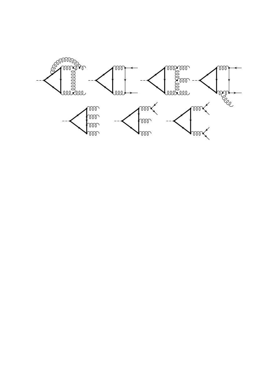
Figure 1: Typical diagrams generating ${\cal O}(\alpha_{s}^{2})$ corrections to $\Gamma(H\to gg)$. Bold-faced (dashed) lines represent the top quark (Higgs boson).

Our procedure is similar to that of Ref. [12]. We construct an effective Lagrangian, ${\cal L}_{\rm eff}$, by integrating out the top quark. This Lagrangian is a linear combination of certain dimension-four operators acting in QCD with five quark flavours, while all $M_{t}$ dependence is contained in the coefficient functions. We then renormalize this Lagrangian and compute with it the $H\to gg$ decay width through ${\cal O}(\alpha_{s}^{4})$. For brevity, we do not list here all operators that enter our analysis in intermediate steps. Instead, we immediately proceed to the final version of ${\cal L}_{\rm eff}$,

$${\cal L}_{\rm eff}=-2^{1/4}G_{F}^{1/2}HC_{1}\left[O_{1}^{\prime}\right].$$ (3)

Here, $\left[O_{1}^{\prime}\right]$ is the renormalized counterpart of the bare operator $O_{1}^{\prime}=G_{a\mu\nu}^{0\prime}G_{a}^{0\prime\mu\nu}$, where $G_{a\mu\nu}$ is the colour field strength, the superscript 0 denotes bare fields, and primed objects refer to the five-flavour effective theory. $C_{1}$ is the corresponding renormalized coefficient function, which carries all $M_{t}$ dependence. Note that $C_{1}$ and $\left[O_{1}^{\prime}\right]$ are not separately renormalization-group (RG) invariant through the order considered, while their product is. From Eq. (3) we may derive a general expression for the $H\to gg$ decay width,

$$\Gamma(H\to gg)=\frac{\sqrt{2}G_{F}}{M_{H}}C_{1}^{2}{\rm Im}\,\langle\left[O_{1}^{\prime}\right]\left[O_{1}^{\prime}\right]\rangle,$$ (4)

where $\langle\left[O_{1}^{\prime}\right]\left[O_{1}^{\prime}\right]\rangle$ is the vacuum polarization of the Higgs field induced by the gluon operator at $q^{2}=M_{H}^{2}$, with $q$ being the external four-momentum.

In order to cope with the enormous complexity of the problem at hand, we make successive use of powerful symbolic manipulation programs. Specifically, we generate the contributing diagrams with the package QGRAF [14] and convert the output to a form that can be used as input for the packages MINCER [15] and MATAD [16], which solve massless and massive three-loop integrals, respectively. The cancellation of the ultraviolet singularities, the gauge-parameter independence, and the RG invariance serve as strong checks for our calculation.

We adopt two independent methods to calculate $C_{1}$. One is based on the LET [13] and naturally extends the analysis of Ref. [12] by one order in $\alpha_{s}$. This leads us to consider the top-quark contributions to the gluon and ghost propagators as well as the gluon-ghost coupling through ${\cal O}(\alpha_{s}^{4})$ with all external four-momenta put to zero. Specifically, we need to compute 189, 25, and 228 three-loop diagrams, respectively. The external Higgs line is then attached through differentiation with respect to the top-quark mass according to the LET. From the resulting three expressions, $C_{1}$ is then obtained by solving a linear set of equations [12]. The second method is the brute-force calculation of the 657 three-loop three-point diagrams which contribute to $C_{1}$. Both methods lead to the same result, which upon renormalization reads

$$C_{1} = -\frac{1}{12}\,\frac{\alpha_{s}^{(6)}(\mu)}{\pi}\left\{1+\frac{\alpha_{s}^{(6)}(\mu)}{\pi}\left(\frac{11}{4}-\frac{1}{6}\ln\frac{\mu^{2}}{M_{t}^{2}}\right)\right.$$ (5)

$$+ \left.\left(\frac{\alpha_{s}^{(6)}(\mu)}{\pi}\right)^{2}\left[\frac{2693}{288}-\frac{25}{48}\ln\frac{\mu^{2}}{M_{t}^{2}}+\frac{1}{36}\ln^{2}\frac{\mu^{2}}{M_{t}^{2}}+n_{l}\left(-\frac{67}{96}+\frac{1}{3}\ln\frac{\mu^{2}}{M_{t}^{2}}\right)\right]\right\},$$

where $\alpha_{s}$ is defined in the $\overline{\rm MS}$ scheme and $M_{t}$ is the top-quark pole mass. Since $C_{1}$ appears as an overall factor in ${\cal L}_{\rm eff}$, it also enters the calculation of the $gg\to H$ parton-level cross section at next-to-leading order [9]. We should mention that Eq. (5) disagrees with the corresponding result recently found in Ref. [9], although the numerical difference is relatively small.

In fact, Eq. (5) can be obtained from known results via the following all-order generalization [17] of the LET:

$$C_{1}=-\frac{\pi}{2\alpha_{s}^{(5)}}\left(\frac{\displaystyle\beta^{(6)}(\alpha_{s}^{(6)})\frac{\partial}{\partial\alpha_{s}^{(6)}}\alpha_{s}^{(5)}-\beta^{(5)}(\alpha_{s}^{(5)})}{1-2\gamma^{(6)}_{m}(\alpha_{s}^{(6)})}\right){}.$$ (6)

Here $\alpha_{s}^{(6)}=\alpha_{s}^{(6)}(\mu)$ and $\alpha_{s}^{(5)}$ should be understood as expressed through $\alpha_{s}^{(6)}(\mu)$ via the decoupling relation [18]

$$\frac{\alpha_{s}^{(5)}(\mu)}{\alpha_{s}^{(6)}(\mu)}=1-\frac{\alpha^{(6)}_{s}(\mu)}{\pi}\left(\frac{1}{6}l_{m}\right)+\left(\frac{\alpha^{(6)}_{s}(\mu)}{\pi}\right)^{2}\left(\frac{11}{72}-\frac{11}{24}l_{m}+\frac{1}{36}l^{2}_{m}\right)+{\cal O}(\alpha_{s}^{3}){},$$ (7)

with $l_{m}=\ln\frac{\mu^{2}}{m^{2}_{t}(\mu)}$ and $m_{t}(\mu)$ being the running top quark mass. Futhermore,

$$\beta^{(n_{f})}(\alpha^{(n_{f})}_{s}) = -\frac{\alpha^{(n_{f})}_{s}}{\pi}\left\{\left(11-\frac{2}{3}~{}n_{{f}}\right)\frac{\alpha^{(n_{f})}_{s}}{4\pi}+\left(102-\frac{38}{3}~{}n_{{f}}\right)\left(\frac{\alpha^{(n_{f})}_{s}}{4\pi}\right)^{2}\right.$$ (8)

$$+ \left.\left(\frac{2857}{2}-\frac{5033}{18}~{}n_{{f}}+\frac{325}{54~{}}~{}n_{{f}}^{2}\right)\left(\frac{\alpha^{(n_{f})}_{s}}{4\pi}\right)^{3}+{\cal O}(\alpha_{s}^{4})\right\}$$

and

$$\gamma^{(n_{f})}(\alpha_{s}^{(n_{f})})=-\frac{\alpha^{(n_{f})}_{s}}{\pi}-\left(\frac{202}{3}-\frac{20}{9}~{}n_{{f}}\right)\left(\frac{\alpha^{(n_{f})}_{s}}{4\pi}\right)^{2}+{\cal O}(\alpha_{s}^{3})$$ (9)

stand for the $\overline{\rm MS}$ beta-function [19] and the quark anomalous dimension [20], respectively. Eq. (5) is then recovered from Eq. (6) by expressing $m_{t}(\mu)$ in terms of $M_{t}$ according to [21].

We now turn to the second unknown ingredient in Eq. (4), ${\rm Im}\,\langle\left[O_{1}^{\prime}\right]\left[O_{1}^{\prime}\right]\rangle$. In fact, it is convenient to calculate $\langle\left[O_{1}^{\prime}\right]\left[O_{1}^{\prime}\right]\rangle$ first and then to take the absorptive part of it. There is a total of 403 three-loop diagrams to be evaluated. After renormalization, the result is

$${\rm Im}\,\langle\left[O_{1}^{\prime}\right]\left[O_{1}^{\prime}\right]\rangle = (q^{2})^{2}\frac{2}{\pi}\left\{1+\frac{\alpha_{s}^{(n_{l})}(\mu)}{\pi}\left[\frac{73}{4}+\frac{11}{2}\ln\frac{\mu^{2}}{q^{2}}-n_{l}\left(\frac{7}{6}+\frac{1}{3}\ln\frac{\mu^{2}}{q^{2}}\right)\right]\right.$$ (10)

$$+ \left(\frac{\alpha_{s}^{(n_{l})}(\mu)}{\pi}\right)^{2}\left[\frac{37631}{96}-\frac{363}{8}\zeta(2)-\frac{495}{8}\zeta(3)+\frac{2817}{16}\ln\frac{\mu^{2}}{q^{2}}+\frac{363}{16}\ln^{2}\frac{\mu^{2}}{q^{2}}\right.$$

$$+ n_{l}\left(-\frac{7189}{144}+\frac{11}{2}\zeta(2)+\frac{5}{4}\zeta(3)-\frac{263}{12}\ln\frac{\mu^{2}}{q^{2}}-\frac{11}{4}\ln^{2}\frac{\mu^{2}}{q^{2}}\right)$$

$$+ \left.\left.n_{l}^{2}\left(\frac{127}{108}-\frac{1}{6}\zeta(2)+\frac{7}{12}\ln\frac{\mu^{2}}{q^{2}}+\frac{1}{12}\ln^{2}\frac{\mu^{2}}{q^{2}}\right)\right]\right\},$$

where $\zeta$ is Riemann’s zeta function, with values $\zeta(2)=\pi^{2}/6$ and $\zeta(3)\approx 1.202$.

We are now in a position to find the ${\cal O}(\alpha_{s}^{2})$ term of the $K$ factor in Eq. (2). To this end, we insert Eqs. (5) and (10) with $q^{2}=M_{H}^{2}$ into the master formula (4) and factor out the Born result of Eq. (1). In order to get a compact expression, we also eliminate $\alpha_{s}^{(6)}(\mu)$ in favour of $\alpha_{s}^{(n_{l})}(\mu)$ [18] and choose $\mu=M_{H}$. We thus obtain

$$K = 1+\frac{\alpha_{s}^{(n_{l})}(M_{H})}{\pi}\left(\frac{95}{4}-\frac{7}{6}n_{l}\right)+\left(\frac{\alpha_{s}^{(n_{l})}(M_{H})}{\pi}\right)^{2}\left[\frac{149533}{288}-\frac{363}{8}\zeta(2)-\frac{495}{8}\zeta(3)\right.$$ (11)

$$- \left.\frac{19}{8}\ln\frac{M_{t}^{2}}{M_{H}^{2}}+n_{l}\left(-\frac{4157}{72}+\frac{11}{2}\zeta(2)+\frac{5}{4}\zeta(3)-\frac{2}{3}\ln\frac{M_{t}^{2}}{M_{H}^{2}}\right)+n_{l}^{2}\left(\frac{127}{108}-\frac{1}{6}\zeta(2)\right)\right]$$

$$\approx 1+17.917\,\frac{\alpha_{s}^{(5)}(M_{H})}{\pi}+\left(\frac{\alpha_{s}^{(5)}(M_{H})}{\pi}\right)^{2}\left(156.808-5.708\,\ln\frac{M_{t}^{2}}{M_{H}^{2}}\right),$$

where we have substituted $n_{l}=5$ in the last step. If we also use the measured values $M_{t}=175$ GeV and $\alpha_{s}^{(5)}(M_{Z})=0.118$, and assume $M_{H}=100$ GeV, we have

$$K \approx 1+17.917\,\frac{\alpha_{s}^{(5)}(M_{H})}{\pi}+150.419\,\left(\frac{\alpha_{s}^{(5)}(M_{H})}{\pi}\right)^{2}$$ (12)

$$\approx 1+0.66+0.21.$$

We observe that the new ${\cal O}(\alpha_{s}^{2})$ term further increases the well-known ${\cal O}(\alpha_{s})$ enhancement by about one third. If we assume that this trend continues to ${\cal O}(\alpha_{s}^{3})$ and beyond, then Eq. (11) may already be regarded as a useful approximation to the full result. Inclusion of the new ${\cal O}(\alpha_{s}^{2})$ correction leads to an increase of the Higgs-boson hadronic width by an amount of order 1%.

Equation (11) may be RG-improved by resumming the terms proportional to $\ln(M_{t}^{2}/M_{H}^{2})$ as described in Ref. [12]. This leads to

$$K \approx 1+14.938\,\frac{\alpha_{s}^{(5)}(M_{H})}{\pi}+2.978\,\frac{\alpha_{s}^{(6)}(M_{t})}{\pi}+104.499\,\left(\frac{\alpha_{s}^{(5)}(M_{H})}{\pi}\right)^{2}$$ (13)

$$+ 44.491\,\frac{\alpha_{s}^{(5)}(M_{H})}{\pi}\,\frac{\alpha_{s}^{(6)}(M_{t})}{\pi}+7.818\,\left(\frac{\alpha_{s}^{(6)}(M_{t})}{\pi}\right)^{2}.$$

For the $M_{H}$ values of interest here (65.6 GeV${}<M_{H}\ll 2M_{t}$), this amounts to an insignificant reduction of the absolute value of $K$, by at most 0.6%, for $M_{H}=65.6$ GeV. In particular, the second line of Eq. (12) remains valid within its accuracy.

Finally, we wish to mention that the $K$ factor of Eq. (11) also applies to the neutral CP-even Higgs bosons of two-Higgs-doublet models such as the minimal supersymmetric extension of the standard model, as long as their couplings to gluon pairs are dominantly generated via top-quark loops.

We thank Paolo Nogueira for beneficial communications concerning Ref. [14].

References

• [1] P. Janot, in Proceedings of the Ringberg Workshop: The Higgs Puzzleβ€”What can we learn from LEP2, LHC, NLC, and FMC?, Rottach-Egern, Germany, 8–13 December 1996, edited by B.A. Kniehl (World Scientific, Singapore, in press).
• [2] M. Boutemeur, in Ref.Β [1].
• [3] F. Wilczek, Phys.Β Rev.Β Lett.Β 39, 1304 (1977).
• [4] M. Veltman, Nucl.Β Phys.Β B123, 89 (1977).
• [5] L.D. Landau, Dokl.Β Akad.Β Nauk USSR 60, 207 (1948); C.N. Yang, Phys.Β Rev.Β 77, 242 (1949).
• [6] H.M. Georgi, S.L. Glashow, M.E. Machacek, and D.V. Nanopoulos, Phys.Β Rev.Β Lett.Β 40, 692 (1978).
• [7] S. Dawson, Nucl.Β Phys.Β B359, 283 (1991); S. Dawson and R.P. Kauffman, Phys.Β Rev.Β Lett.Β 68, 2273 (1992); Phys.Β Rev.Β D 49, 2298 (1994); D. Graudenz, M. Spira, and P.M. Zerwas, Phys.Β Rev.Β Lett.Β 70, 1372 (1993); M. Spira, A. Djouadi, D. Graudenz, and P.M. Zerwas, Nucl.Β Phys.Β B453, 17 (1995).
• [8] A. Djouadi, M. Spira, and P.M. Zerwas, Phys.Β Lett.Β B 264, 440 (1991).
• [9] M. KrΓ€mer, E. Laenen, and M. Spira, Report Nos.Β CERN–TH/96–231, DESYΒ 96–170, and hep–ph/9611272 (November 1996).
• [10] E. Gross, B.A. Kniehl, and G. Wolf, Z. Phys.Β C 63, 417 (1994); 66, 321(E) (1995).
• [11] A. Djouadi, M. Spira, and P.M. Zerwas, Z. Phys.Β C 70, 427 (1996).
• [12] T. Inami, T. Kubota, and Y. Okada, Z. Phys.Β C 18, 69 (1983).
• [13] J. Ellis, M.K. Gaillard, and D.V. Nanopoulos, Nucl.Β Phys.Β B106, 292 (1976); A.I. VaΔ­nshteΔ­n, M.B. Voloshin, V.I. Zakharov, and M.A. Shifman, Yad.Β Fiz.Β 30, 1368 (1979) [Sov.Β J. Nucl.Β Phys.Β 30, 711 (1979)]; A.I. VaΔ­nshteΔ­n, V.I. Zakharov, and M.A. Shifman, Usp.Β Fiz.Β Nauk 131, 537 (1980) [Sov.Β Phys.Β Usp.Β 23, 429 (1980)]; M.B. Voloshin, Yad.Β Fiz.Β 44, 738 (1986) [Sov.Β J. Nucl.Β Phys.Β 44, 478 (1986)]; B.A. Kniehl and M. Spira, Z. Phys.Β C 69, 77 (1995).
• [14] P. Nogueira, J. Comput.Β Phys.Β 105, 279 (1993).
• [15] S.A. Larin, F.V. Tkachev, and J.A.M. Vermaseren, NIKHEF Report No.Β NIKHEF–H/91–18 (September 1991).
• [16] M. Steinhauser, Ph.D. thesis, Karlsruhe University (Shaker Verlag, Aachen, 1996).
• [17] K.G. Chetyrkin, B.A. Kniehl and M. Steinhauser, in preparation.
• [18] S.A. Larin, T. van Ritbergen, and J.A.M. Vermaseren, Nucl.Β Phys.Β B438, 278 (1995).
• [19] O.V. Tarasov, A.A. Vladimirov, A.Yu. Zharkov, Phys.Β Lett.Β B 93 (1980) 429; S.A. Larin and J.A.M. Vermaseren, Phys. Lett. B 303 (1993) 334.
• [20] R. Tarrach, Nucl. Phys. B 183 (1981) 384.
• [21] N. Gray, D.J. Broadhurst, W. Grafe and K. Schilcher, Z. Phys. C 48 (1990) 673.