DTP/97/32

hep-ph/9705229

May 1997

Hadronic Antenna Patterns as a Probe of
Leptoquark Production at HERA

M. Heyssler^a and W. J. Stirling^a,b

${}^{a}\;$ Department of Physics, University of Durham, Durham, DH1 3LE

${}^{b}\;$ Department of Mathematical Sciences, University of Durham, Durham, DH1 3LE

Hadronic antenna patterns can provide a valuable diagnostic tool for probing the origin of the apparent excess of high $x,Q^{2}$ events at HERA. We present quantitative predictions for the distributions of soft particles and jets in standard deep inelastic scattering $eq\to eq$ events and in events corresponding to the production of a narrow colour–triplet scalar (‘leptoquark’) resonance. The corresponding distributions of soft photon radiation, which are sensitive to the leptoquark electric charge, are also presented. The distribution for one particular leptoquark assignment is shown to contain a radiation zero.

1 Introduction

The observation of an apparent excess of deep inelastic scattering events in positron–proton collisions at high $Q^{2}$ by both the H1 [1] and ZEUS [2] collaborations at HERA has prompted much speculation about possible new physics explanations. Obvious candidates are a new four–fermion contact interaction $\Lambda^{-2}\bar{e}e\bar{q}q$ with $\Lambda\sim{\cal O}(1-2\;{\rm TeV})$, or the production of a new heavy ‘leptoquark’ resonance $e^{+}q\to{\rm LQ}\to e^{+}q$ with $M_{\rm LQ}\sim 200\;{\rm GeV}$ [3]. The electric charge of such an object is not yet known, but if $e_{{\rm LQ}}=+2/3$, corresponding to $e^{+}d\to{\rm LQ}$ for example, then the new particle could be a heavy squark in an $R$–parity violating supersymmetric extension of the Standard Model.

It is important to investigate all possible ways in which one could distinguish between a conventional explanation (i.e. a fluctuation of the standard model DIS process) and new physics scenarios. One diagnostic tool which has already been advocated [4] in the context of large $E_{T}$ jet production at hadron colliders is to use the pattern of hadronic energy flow in the event [References–References]. This is based on the idea [5, 6] that the overall structure of particle angular distributions in a hard scattering process (the ‘event portrait’ or ‘antenna pattern’) is governed by the underlying colour dynamics at short distance. Thus the event portrait can be regarded as a ‘partonometer’ [4] mapping the basic scattering process.

The events at high $x$ and $Q^{2}$ at HERA seem ideally suited to such a study, being characterized by an energetic, well–separated lepton and jet in the final state. Furthermore the various candidate underlying $eq\to eq$ processes ($t$–channel $\gamma^{*},Z$ exchange, contact interaction, $s$–channel colour–triplet resonance production, …) have distinctive antenna patterns, as we shall see. In practice one could, with sufficiently high statistics, use an additional soft (gluon) jet as a probe of the antenna pattern. With fewer events the distribution of soft hadrons can be used instead. Both of these quantities are related to the inclusive soft gluon distribution in the next–to–leading order $eq\to eqg$ processes, the former directly and the latter through the hypothesis of Local Parton Hadron Duality (LPHD) [14] in which the angular distribution of soft particles emitted at wide angles to the energetic jets follows that of the underlying soft partons, with the rate being determined by overall multiplicative energy–dependent cascading factors [5, 15].

The idea, then, is to use the angular distributions of soft particles or jets as a probe of new physics contributions to high–$Q^{2}$ $e^{+}q$ scattering. We imagine a situation where a larger sample of (presumably standard model DIS) events at slightly lower $Q^{2}$ is used as a control, to check the approximate validity of our quantitative predictions for the antenna pattern. This can then be compared with the observed antenna pattern for the sample of excess events. As we shall see, in some cases the ‘signal’ and ‘background’ distributions can differ by factors of 2 or more. The variation of the patterns with the DIS variable $y$ will also be a useful discriminant.

We should also remark that experimental support for the feasibility of such antenna pattern studies has come recently from the CDF and D0 collaborations at the Tevatron $p\bar{p}$ collider [16, 17]. Their analyses have shown that distinctive colour interference effects in multijet and $W+$jet production survive the hadronization phase and are clearly visible in the data.

In the following section we derive the basic antenna pattern results for standard DIS and leptoquark production. The case of a new contact interaction is obtained as a limiting case of the latter. In Section 3 we present numerical predictions for various typical kinematic configurations. Analogous results for soft photon production are obtained in Section 4, and Section 5 contains our conclusions.

2 Antenna patterns for deep inelastic scattering and leptoquark production

The distribution of soft gluon radiation is controlled by the basic antenna pattern (see for example Ref. [7])

$$[ij]\equiv{p_{i}\cdot p_{j}\over p_{i}\cdot k\;p_{j}\cdot k}={1-{\bf n}_{i}\cdot{\bf n}_{j}\over\omega^{2}(1-{\bf n}\cdot{\bf n}_{i})\;(1-{\bf n}\cdot{\bf n}_{j})}\;,$$ (1)

where the $p_{i}^{\mu}=E_{i}(1,{\bf n}_{i})$ are the four–momenta of the energetic quarks and leptons participating in the hard scattering process, and $k^{\mu}=\omega(1,{\bf n})$ is the four–momentum of the soft gluon. The radiation patterns presented below correspond to the $\omega/E_{i}\to 0$ limits of the exact $eq\to eqg$ matrix elements.

We start by considering the Standard Model process $e(p_{1})+q(p_{2})\to e(p_{3})+q(p_{4})$ by $t$–channel $\gamma^{*},Z$ exchange. If the invariant mass of the $eq$ system is $M$, and if the angle between the incoming and outgoing quarks (in the $eq$ c.m.s. frame) is $\Theta_{q}$, i.e. $\cos\Theta_{q}={\bf n}_{2}\cdot{\bf n}_{4}$, then the usual DIS variables are

$$x=\frac{M^{2}}{s}\;,\quad y=\frac{1}{2}(1-\cos\Theta_{q})\;,\quad Q^{2}=yM^{2}\;.$$ (2)

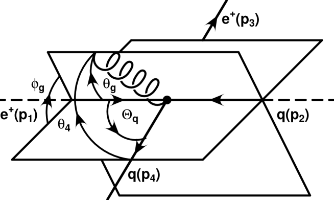
Figure 1: Parametrization of the kinematics for $e^{+}(p_{1})q(p_{2})\rightarrow e^{+}(p_{3})q(p_{4})+g(k)$ scattering in the $e^{+}q$ c.m.s. frame. The orientation of the soft gluon relative to the scattering plane is denoted by $\theta_{g}$ and $\phi_{g}$ or, alternatively, by the angles with respect to the directions of the participating quarks: $\theta_{4}$ and $\theta_{2}=\theta_{g}$.

The scattering process with the various momenta labelled is shown in Fig. 1.

Since our aim is to distinguish the patterns for resonance production and the normal deep inelastic scattering, we consider fixed $M$ and variable $\Theta_{q}$ ($y$). For the Standard Model process the gluon energy and angular distribution is simply (see for example [7])

$$\frac{1}{\sigma_{0}}{d\sigma\over d\omega d\Omega_{\bf n}}={\alpha_{s}C_{F}\over 4\pi^{2}}\;\omega\;{\cal F}_{\rm SM}$$ (3)

where

$${\cal F}_{\rm SM}=2[24]={2p_{2}\cdot p_{4}\over p_{2}\cdot k\;p_{4}\cdot k}={2(1-\cos\Theta_{q})\over\omega^{2}(1-\cos\theta_{2})\;(1-\cos\theta_{4})}\;,$$ (4)

where $\cos\theta_{i}={\bf n}\cdot{\bf n}_{i}$ denotes the angle between the soft gluon and the corresponding quark. The gluon emission is coherent, and depends on the relative orientation of the incoming and outgoing quark directions. Eq. (4) can be interpreted as a colour ‘string’ connecting the incoming and outgoing quarks [15, 18], and is closely related to the familiar result ${\cal F}=2[q\bar{q}]$ for the crossed process $e^{+}e^{-}\to q\bar{q}$ (see for example [7]).

We now turn to the radiation pattern corresponding to the production of an unstable colour–triplet, $s$–channel scalar resonance ${\rm LQ}$ of mass $M$ and decay width $\Gamma$, i.e. $eq\to{\rm LQ}\to eq$. We first note that the emission of a soft gluon off an on–shell colour–triplet scalar boson is described by the same factor as emission off a colour–triplet fermion, i.e.

$${\cal M}^{(1)}\simeq{\cal M}^{(0)}\;T^{a}_{ij}g_{s}{P\cdot\epsilon_{\lambda}^{a}(k)\over P\cdot k}\;,$$ (5)

where $T^{a}$ is a SU(3) colour matrix, $P^{\mu}$ is the momentum of the emitting particle, and $\epsilon^{a}_{\lambda}$ is the gluon polarization vector. We can therefore use results already obtained for heavy quark production and decay [References,References,References–References] to write down the result for leptoquark production and decay:

$${\cal F}_{\rm LQ}=2\left([2P]+[4P]-[PP]\right)+2\chi\left([PP]+[24]-[2P]-[4P]\right)$$ (6)

where $P=p_{1}+p_{2}$ is the leptoquark momentum. The factor $\chi$ in (6) is given by

$$\chi={M^{2}\Gamma^{2}\over(P\cdot k)^{2}+M^{2}\Gamma^{2}}={\Gamma^{2}\over\omega^{2}+\Gamma^{2}}$$ (7)

where the second expression corresponds to the ${\rm LQ}$ c.m.s. frame. As discussed at length in Ref. [21], the radiation pattern depends, through the factor $\chi$, on the relative size of the gluon energy and the leptoquark decay width. In this respect it is instructive to consider the two (formal) limits $\Gamma\to\infty$ ($\chi\to 1$) and $\Gamma\to 0$ ($\chi\to 0$), for fixed $\omega$. In the former, the leptoquark decays immediately after it is produced and has no time to radiate gluons of wavelength $\sim 1/\omega$. In this limit

$${\cal F}_{\rm LQ}\rightarrow 2[24]\;,$$ (8)

which is identical to the standard DIS pattern (4) corresponding to coherent emission. In contrast, for $\Gamma/\omega\to 0$ the emission takes place on two very different timescales, corresponding to the production stage and the decay stage [21]:

$${\cal F}_{\rm LQ}\rightarrow\left\{2[2P]-[PP]\right\}+\left\{2[4P]-[PP]\right\}\;.$$ (9)

At threshold, where there is essentially no radiation from the heavy leptoquark, the two terms in $\{\}$ correspond to independent radiation off the initial and final state (massless) quarks, see (11) below. Note that it is straightforward to verify that the first term on the right–hand side of (9) does indeed correspond to the $k^{\mu}\to 0$ limit of the real gluon emission matrix element squared for $e+q\to{\rm LQ}+g$ calculated in Refs. [24, 25].

With no a priori knowledge of the decay width of the new heavy particle, the antenna pattern (6) could in principle be used to obtain a measurement. This was the approach advocated in Ref. [21] for the top quark. As we shall see in the following section, in certain regions of phase space the antenna pattern is very sensitive to $\chi$, and therefore to $\Gamma$. In practice, it seems that for the class of leptoquark models proposed [3] to explain the excess of high–$Q^{2}$ events at HERA, the decay width is rather small. In particular, a scalar leptoquark coupling with strength $\lambda$ to $eq$ has a corresponding decay width $\Gamma=M\lambda^{2}/(16\pi)$. For ‘first generation’ leptoquarks values of $\lambda^{2}<{\cal O}(10^{-2})$ are allowed by low–energy data (see for example Ref. [24] and references therein). This implies that such resonances should be very narrow, i.e. $\Gamma<{\cal O}(40\;{\rm MeV})$ for $M\sim 200\;{\rm GeV}$. If we are interested in the distributions of soft hadrons or jets with energies of order a few GeV, then $\chi\ll 1$ and (9) is the appropriate distribution for the leptoquark signal.

Finally, we note that the antenna pattern for a $\bar{e}e\bar{q}q$ contact interaction corresponds to the limit $\chi\to 1$, and is therefore identical to the standard DIS result, Eq. (4).

3 Numerical results

In this section we present numerical results for the standard model DIS and leptoquark soft gluon distributions. We work in the $eq$ c.m.s. frame with angles defined as in Fig. 1, and focus on the dependence of the dimensionless quantity ${\cal N}=\omega^{2}{\cal F}$, where ${\cal F}_{\rm SM}$ and ${\cal F}_{\rm LQ}$ are defined in (4) and (9) respectively, on the gluon direction ${\bf n}$. Simple algebra gives

$${\cal N}_{\rm SM} = {2(1-\cos\Theta_{q})\over(1-\cos\theta_{2})(1-\cos\theta_{4})}\;,$$ (10)

$${\cal N}_{\rm LQ} = {1+\cos\theta_{2}\over 1-\cos\theta_{2}}+{1+\cos\theta_{4}\over 1-\cos\theta_{4}}\;,$$ (11)

$${{\cal N}_{\rm LQ}\over{\cal N}_{\rm SM}} = {1-\cos\theta_{2}\cos\theta_{4}\over 1-\cos\Theta_{q}}\;.$$ (12)

The patterns and their ratio are displayed in Figs. 2 and 3, as functions of $\theta_{g}$ and $\phi_{g}$, the polar and azimuthal gluon angles with respect to the incoming quark direction, and for fixed values of $\Theta_{q}=45^{\circ},90^{\circ},135^{\circ}$, i.e. $y=0.146,0.5,0.854$. To avoid the collinear–singular regions of phase space, cuts $\theta_{2},\theta_{4}>10^{\circ}$ are imposed.

We note the following points:

• For the standard model distribution, there is a significant enhancement of radiation in the region between the quark directions (i.e. $\phi\sim 0^{\circ},\;0^{\circ}\lower 3.01385pt\hbox{$\;\stackrel{{\scriptstyle\textstyle<}}{{\sim}}\;$}\theta\lower 3.01385pt\hbox{$\;\stackrel{{\scriptstyle\textstyle<}}{{\sim}}\;$}\Theta_{q}$), as expected. This enhancement is largely absent in the ${\rm LQ}$ case, where the radiation pattern is simply a superposition of independent radiation off the initial and final state quarks.

• In the limit $\Theta_{q}\to 0^{\circ}$, ${\cal N}_{\rm SM}$ vanishes everywhere since the final state comoving colour triplet and antitriplet behave as a colour singlet, whereas ${\cal N}_{\rm LQ}$ is simply twice the radiation off a single quark. In Ref. [22], similar effects where discussed for $e^{+}e^{-}\to t\bar{t}\to W^{+}W^{-}b\bar{b}$ production at threshold.

• For $\Theta_{q}=90^{\circ}$ scattering, the ratio of the SM and ${\rm LQ}$ distributions achieves its minimum and maximum values in the plane of the scattering, thus ${\cal N}_{\rm LQ}=\frac{1}{2}{\cal N}_{\rm SM}$ for $(\phi_{g},\theta_{g})=(0^{\circ},45^{\circ})$ and $(180^{\circ},135^{\circ})$ and ${\cal N}_{\rm LQ}=\frac{3}{2}{\cal N}_{\rm SM}$ for $(\phi_{g},\theta_{g})=(0^{\circ},135^{\circ})$ and $(180^{\circ},45^{\circ})$. The distributions are the same for gluon directions in the planes perpendicular to ${\bf n}_{2}$ and ${\bf n}_{4}$, i.e. $\theta_{2},\theta_{4}=90^{\circ}$.

Finally, from the above discussion we would expect that the azimuthal distribution of soft gluons (hadrons) around the final state quark (jet) direction would be more uniform for quarks from leptoquark decay than from standard deep inelastic scattering. To see this, we show in Fig. 4 the azimuthal $\tilde{\phi}_{g}$ distribution of the gluon around the final state quark direction ${\bf n}_{4}$, for $\Theta_{q}=90^{\circ}$ and various fixed $\theta_{4}$. A significant azimuthal asymmetry for ${\cal N}_{\rm SM}$ is observed with a maximum in the plane of the scattering between the quark directions ($\tilde{\phi}_{g}=0^{\circ}$), as expected. In contrast, the dependence of ${\cal N}_{\rm LQ}$ on $\tilde{\phi}_{g}$ is very weak, particularly for small $\theta_{4}$.

4 Soft photon emission

As discussed in the introduction, it would be of considerable interest in distinguishing new physics models of the HERA high–$Q^{2}$ events to know the electric charge of the quarks in the $eq\to eq$ process. In principle, this information is contained in the distribution of soft photon radiation, which can be obtained in an analogous way to the soft gluon distributions of Section 2. The main difference is the presence of additional contributions from emission off the incoming and outgoing positrons. The result is (cf. Eqs. (3,4,6))

$$\frac{1}{\sigma_{0}}{d\sigma\over d\omega_{\gamma}d\Omega_{\bf n}}={\alpha\over 4\pi^{2}}\;\omega_{\gamma}\;{\cal F}^{\gamma}$$ (13)

where

$${\textstyle{1\over 2}}{\cal F}_{\rm SM}^{\gamma} = e_{q}^{2}[24]-e_{q}\{[12]+[34]-[14]-[23]\}+[13]$$ (14)

$${\textstyle{1\over 2}}{\cal F}_{\rm LQ}^{\gamma} = e_{q}(1+e_{q})\{[2P]+[4P]\}+(1+e_{q})\{[1P]+[3P]\}$$ (15)

$$-e_{q}\{[12]+[34]\}-(1+e_{q})^{2}[PP]$$

$$+\chi\Bigl{(}(1+e_{q})^{2}[PP]-e_{q}(1+e_{q})\{[2P]+[4P]\}$$

$$-(1+e_{q})\{[1P]+[3P]\}+e_{q}^{2}[24]+e_{q}\{[14]+[23]\}+[13]\Bigr{)}$$

and, as before, ${\cal F}_{\rm SM}^{\gamma}={\cal F}_{\rm LQ}^{\gamma}(\chi=1)$. As argued in the previous section, it is the $\chi\to 0$ limit of ${\cal F}_{\rm LQ}^{\gamma}$ which is relevant in practice, i.e. for photons with energy $\omega_{\gamma}\gg\Gamma_{{\rm LQ}}$. In this limit we have

$${\textstyle{1\over 2}}{\cal F}_{\rm LQ}^{\gamma} = e_{q}(1+e_{q})\{[2P]+[4P]\}+(1+e_{q})\{[1P]+[3P]\}$$ (16)

$$-e_{q}\{[12]+[34]\}-(1+e_{q})^{2}[PP]$$

$$=H(\cos\theta_{2})+H(\cos\theta_{4})$$

where

$$H(z)={1\over 1+z}+{e_{q}^{2}\over 1-z}-{\textstyle{1\over 2}}(1+e_{q})^{2}\;.$$ (17)

An interesting feature of the above distributions is the presence of radiation zeros (see for example [26]), i.e. directions of the photon three–momentum ${\bf n}$ for which the cross section vanishes. To see this for the distribution (6) we note that

$$H=0\qquad\mbox{for}\qquad z=z_{0}\equiv{1-e_{q}\over 1+e_{q}}\;.$$ (18)

For the two cases of interest $e_{q}=\frac{2}{3},-\frac{1}{3}$ for which $z_{0}=\frac{1}{5},2$. Therefore only for $e^{+}u$ scattering is the radiation zero in the physical region. For the full distribution (16) to vanish we obviously require

$$\cos\theta_{2}=\cos\theta_{4}=z_{0}\;.$$ (19)

Thus for $e^{+}u$ scattering the radiation zero is in the direction given by the intersection of the two cones of half–angle $\theta_{0}=\cos^{-1}(1/5)=78.46^{\circ}$ centred on the quark directions ${\bf n}_{2}$ and ${\bf n}_{4}$. Three cases can be distinguished:

• For $0^{\circ}<\Theta_{q}<2\theta_{0}$ there are two solutions, corresponding to

  $$\theta_{\gamma}=\theta_{0}\;,\qquad\phi_{\gamma}=\pm\cos^{-1}\left({\tan(\Theta_{q}/2)\over\tan\theta_{0}}\right)\;.$$ (20)

• For $\Theta_{q}=2\theta_{0}$ there is one solution,

  $$\theta_{\gamma}=\theta_{0}\;,\qquad\phi_{\gamma}=0^{\circ}\;,$$ (21)

  corresponding to the bisector of the quark directions in the scattering plane.

• For $\Theta_{q}=0^{\circ}$ there is a cone of solutions corresponding to $\theta_{\gamma}=\theta_{0}$.

Although the above results on the location of the radiation zeroes have been derived for the leptoquark radiation pattern, they apply equally well for the standard model distribution (14), or indeed for the generic distribution (15) for arbitrary $\chi$. This follows from the fact that the zeroes are the result of completely destructive interference between the classical electric fields associated with the different charged particles, see for example Ref. [6]. They depend only on the relative orientation of the various particles, irrespective of whether intermediate resonances are formed. The key point to note is that since presumably the leptoquark couples to either $u$ or $d$ but not both, the radiation zero is either fully present or completely absent. In contrast, the standard model background is a linear combination (determined by the parton distributions) of $u$– and $d$–type distributions, giving a dip rather than a zero.

As a numerical illustration of these results, we show in Fig. 5 the antenna patterns ${\cal N}^{\gamma}_{\rm SM}$, ${\cal N}^{\gamma}_{\rm LQ}(e_{q}=2/3)$ and ${\cal N}^{\gamma}_{\rm LQ}(e_{q}=-1/3)$, with $\Theta_{q}=90^{\circ}$. To exhibit the radiation zeroes more clearly, Fig. 6 shows the $\phi_{\gamma}$ dependence of the leptoquark $e_{q}=2/3,-1/3$ distributions at the critical polar angle $\theta_{\gamma}=\theta_{0}$, i.e. the slices through the two–dimensional distributions of Fig. 5 at this value of $\theta_{\gamma}$. The two zeroes of the $e^{+}u$ distribution at the $\phi_{\gamma}$ angles given by Eq. (20) are clearly visible. Note also that the behaviour of the distributions near the positron and the quark jet directions simply reflects the magnitude of the charge of the corresponding particles.

5 Conclusions

If the observation of an excess of high–$Q^{2}$ events at HERA persists, it will be important to devise new analysis techniques for identifying the origin of the excess. In this paper we have shown that the angular distribution of the accompanying hadronic radiation – the antenna pattern – is a potentially powerful tool for discriminating standard deep inelastic scattering events from those arising from the production of a long–lived coloured scalar ‘leptoquark’ resonance. The main qualitative difference is the absence for the latter of an enhancement of hadronic radiation between the incoming and outgoing quark jet directions (string effect), as shown in Fig. 2. It follows that soft hadrons are distributed more uniformly in azimuth around the final state quark jet direction in events where a leptoquark is produced, see Fig. 3. Our quantitative predictions are based on the phenomenologically successful principle of Local Parton Hadron Duality, and should therefore be a good guide to the behaviour of the distributions of soft hadrons and jets in the detectors. Ultimately, however, there will be no substitute for detailed Monte Carlo studies based on parton–shower/hadronization models, provided that these include the correct underlying colour structure.

Finally we have extended our results to include soft photon radiation. Here the distributions have an additional sensitivity to the electric charge of the leptoquark, which is a crucial parameter in distinguishing models. For the case of charge $5/3$ leptoquarks, produced for example in $e^{+}u$ collisions, the soft photon distribution contains radiation zeroes. These are absent for charge $2/3$ leptoquarks produced in $e^{+}d$ collisions.

Acknowledgements

We thank John Ellis and Valery Khoze for useful comments and discussions. This work was supported in part by the UK PPARC and the EU Programme “Human Capital and Mobility”, Network “Physics at High Energy Colliders”, contract CHRX-CT93-0357 (DG 12 COMA). MH gratefully acknowledges financial support in the form of a DAAD-Doktorandenstipendium (HSP III).

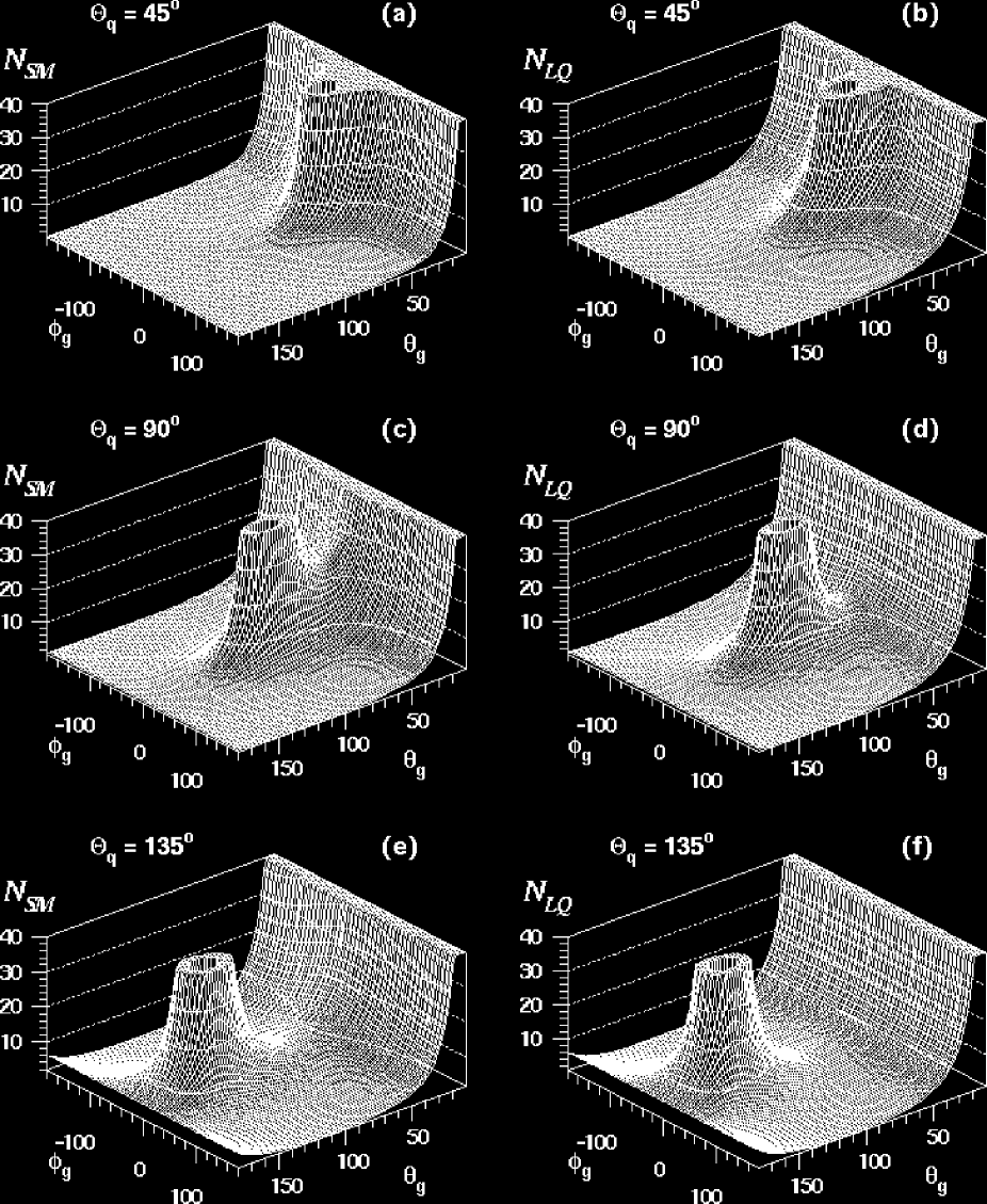
Figure 2: The dimensionless antenna patterns ${\cal N}_{\rm SM}=\omega^{2}{\cal F}_{\rm SM}$ [(a),(c),(e)] and ${\cal N}_{\rm LQ}=\omega^{2}{\cal F}_{\rm LQ}$ [(b),(d),(f)] of Eqs. (10,11) for different c.m.s. scattering angles $\Theta_{q}$ (cf. Fig. 1). Note the cut of $10^{\circ}$ imposed around the incoming and outgoing quark directions.

Figure 3: The ratios ${\cal N}_{\rm LQ}/{\cal N}_{\rm SM}$ of the distributions in Fig. 2 for the three different c.m.s. scattering angles. In this case no angular cuts have been imposed.

Figure 4: The dependence of the antenna patterns ${\cal N}_{\rm SM}$ and ${\cal N}_{\rm LQ}$ on the azimuthal angle $\tilde{\phi}_{g}$ of the soft gluon around the outgoing quark $q(p_{4})$. The gluon direction describes a cone around the quark of half–angle $\theta_{4}$. The direction of the incoming quark $q(p_{2})$ is defined by $\tilde{\phi}_{g}=0^{\circ}$, and the incoming positron $e^{+}(p_{1})$ is at $\tilde{\phi}_{g}=\pm 180^{\circ}$. The overall c.m.s. scattering angle is fixed at $\Theta_{q}=90^{\circ}$.

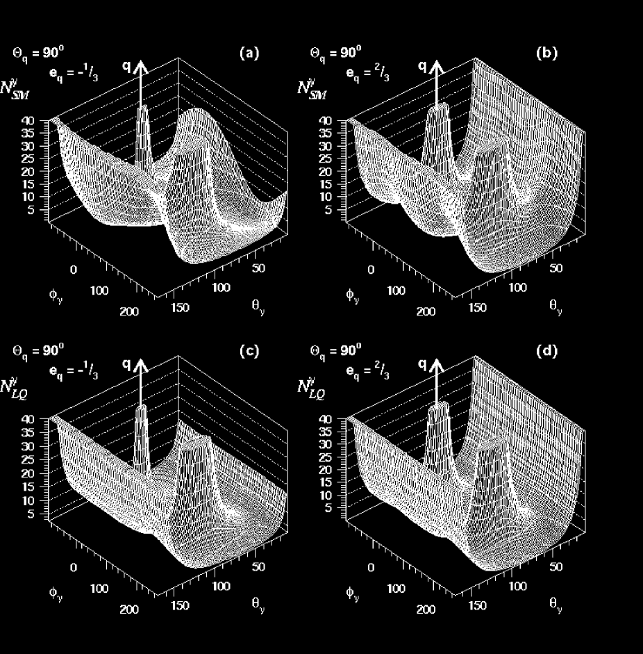
Figure 5: The pattern of soft $\gamma$ radiation according to Eqs. (14,16) with ${\cal N}^{\gamma}_{\rm SM,LQ}=\omega_{\gamma}^{2}{\cal F}^{\gamma}_{\rm SM,LQ}$, for $e^{+}d$ scattering [(a),(c)] and $e^{+}u$ scattering [(b),(d)]. The overall c.m.s. scattering angle is fixed at $\Theta_{q}=90^{\circ}$.

Figure 6: The soft photon antenna pattern ${\cal N}^{\gamma}_{\rm LQ}$ for $\Theta_{q}=90^{\circ}$ at the critical angle $\theta_{\gamma}=\theta_{0}\simeq 78.46^{\circ}$ for $e^{+}u$ (solid line) and $e^{+}d$ (dashed line) scattering. Note the radiation zeros at $\phi_{\gamma}\simeq 78.22^{\circ}$ (cf. Eq. (20)). The positions of the $e^{+}$ and $q$ jets are indicated. Note also that ${\cal N}^{\gamma}_{\rm SM}$ shows quantitatively the same behaviour for this choice of $\theta_{\gamma}$.

References

- [1] H1 Collaboration: C. Adloff et al., DESY preprint 97–24, hep-ex/9702012 (1997).
- [2] ZEUS Collaboration: J. Breitweg et al., DESY preprint 97–25, hep-ex/9702015 (1997).
-
[3]
For a general discussion of the various
new physics possibilities see for example:
G. Altarelli, J. Ellis, G.F. Giudice, S. Lola and M.L. Mangano, preprint CERN–TH/97–40, hep-ph/9703276 (1997).
J.L. Hewett and T.G. Rizzo, SLAC preprint SLAC-PUB-7430, hep-ph/9703337 (1997). - [4] J. Ellis, V.A. Khoze and W.J. Stirling, CERN preprint CERN–TH/96–225, hep-ph/9608486 (1996) to be published in Zeit. Phys.
-
[5]
Yu.L. Dokshitzer, V.A. Khoze and
S.I. Troyan, in Proc. 6th Int. Conf. on Physics in Collision,
ed. M. Derrick (World Scientific, Singapore, 1987), p.417.
Yu.L. Dokshitzer, V.A. Khoze and S.I. Troyan, Sov. J. Nucl. Phys. 46 (1987) 712. -
[6]
Yu.L. Dokshitzer, V.A. Khoze,
A.H. Mueller and S.I. Troyan, Rev. Mod. Phys. 60 (1988) 373.
Yu.L. Dokshitzer, V.A. Khoze and S.I. Troyan in: Advanced Series on Directions in High Energy Physics, Perturbative Quantum Chromodynamics, ed. A.H. Mueller (World Scientific, Singapore), v. 5 (1989) 241. - [7] Yu.L. Dokshitzer, V.A. Khoze, A.H. Mueller and S.I. Troyan, “Basics of Perturbative QCD”, ed. J. Tran Thanh Van, Editions Frontiéres, Gif-sur-Yvette, 1991.
-
[8]
R.K. Ellis, G. Marchesini and
B.R. Webber, Nucl. Phys. B286 (1987) 643; Erratum
Nucl. Phys. B294 (1987) 1180.
R.K. Ellis, presented at “Les Rencontres de Physique de la Vallee d’Aoste”, La Thuile, Italy, March 1987, preprint FERMILAB–Conf–87/108–T (1987). - [9] Yu.L. Dokshitzer, V.A. Khoze and S.I. Troyan, Sov. J. Nucl. Phys. 50 (1989) 505.
- [10] Yu.L. Dokshitzer, V.A. Khoze and T. Sjöstrand, Phys. Lett. B274 (1992) 116.
- [11] G. Marchesini and B.R. Webber, Nucl. Phys. B330 (1990) 261.
- [12] D. Zeppenfeld, Madison preprint MADPH–95–933 (1996).
- [13] V.A. Khoze and W.J. Stirling, Durham preprint DTP/96/106, hep-ph/9612351 (1996).
- [14] Ya.I. Azimov, Yu.L. Dokshitzer, V.A. Khoze and S.I. Troyan, Z. Phys. C27 (1985) 65; C31 (1986) 213.
- [15] Ya.I. Azimov, Yu.L. Dokshitzer, V.A. Khoze and S.I. Troyan, Phys. Lett. B165 (1985) 147; Sov. J. Nucl. Phys. 43 (1986) 95.
- [16] CDF Collaboration: F. Abe et al., Phys. Rev. D50 (1994) 5562; P. Giannetti, FERMILAB preprint FERMILAB-CONF-94-151-E, presented at the 27th International Conference on High Energy Physics (ICHEP), Glasgow, Scotland, July 1994.
- [17] D0 Collaboration: D.E. Cullen-Vidal, presented at the Annual Divisional Meeting (DPF96) of the APS Division of Particles and Fields, Minneapolis, August 1996, FERMILAB preprint, FERMILAB Conf–96–304–EI (1996); H. Melanson, presented at INFN Eloisatron project 33rd Workshop, Erice, Italy, October 1996.
- [18] B. Andersson, G. Gustafson and T. Sjöstrand, Phys. Lett. B94 (1980) 211.
- [19] G. Jikia, Phys. Lett. B257 (1991) 196.
- [20] Yu.L. Dokshitzer, V.A. Khoze and S.I. Troyan, University of Lund preprint LU–TP–92–10 (1992).
- [21] V.A. Khoze, L.H. Orr and W.J. Stirling, Nucl. Phys. B378 (1992) 413.
- [22] Yu.L. Dokshitzer, V.A. Khoze, L.H. Orr and W.J. Stirling, Nucl. Phys. B403 (1993) 65.
- [23] V.A. Khoze, J. Ohnemus and W.J. Stirling, Phys. Rev. D49 (1994) 1237.
- [24] Z. Kunszt and W.J. Stirling, preprint DTP/97/16, hep-ph/9703427 (1997).
- [25] T. Plehn, H. Spiesberger, M. Spira and P.M. Zerwas, preprint DESY-97-43, hep-ph/9703433 (1997).
- [26] S.J. Brodsky and R.W. Brown, Phys. Rev. Lett. 49 (1982) 966.