COULD ELECTROMAGNETIC CORRECTIONS
SOLVE THE VORTON EXCESS PROBLEM ?

Abstract

The modifications of circular cosmic string loop dynamics due to the electromagnetic self–interaction are calculated and shown to reduce the available phase space for reaching classical vorton states, thereby decreasing their remnant abundance. Use is made of the duality between master–function and Lagrangian formalisms on an explicit model.

]

I Introduction

Most particle physics theories, extensions of the so–called standard model of interactions, suggest that topological defects [1] should have been formed during phase transitions in the early universe [2]. Among those, the most fashionable, because of their ability to solve many cosmological puzzles, are cosmic strings, provided couplings with other particles are such that they are not of the superconducting kind [3]. In the latter case, however, they would not be able to decay into pure gravitational radiation, terminating their life in the form of frozen vorton states which might be so numerous that they would cause a cosmological catastrophe [4, 5, 6]: a rough evaluation of their abundance yields a very stringent constraint of a symmetry breaking scale which, to avoid an excess, should be less than $10^{9}$ GeV, which is incompatible with the idea of them being responsible for galaxy formation and leaving imprints in the cosmic microwave background.

There are many ways out of this vorton excess problem, the most widely accepted relying upon stability considerations: since vortons are centrifugally supported string loop configurations, the origin of the rotation being hidden in the existence of a current, it is legitimate to first ask whether the current itself is stable against decay by quantum tunnelling. This question, however, has not yet been properly addressed, and presumably depends on the particular underlying field model one uses, so that, although it is clearly an important point to be clarified, it will not be considered in this work. Another issue, at a lower level, concerns the classical stability: a rotating string configuration in equilibrium may exhibit unstable perturbation states; if it were the case in general for any equation of state, then one would expect vortons to dissipate somehow, and the problem would be cured [7, 8]. This hope is not however fulfilled by the Witten kind of strings whose equation of state [9, 10] falls into the possibly stable category [11].

Finally, another point worth investigating is that of vorton formation. It should be clear that an arbitrary cosmic string loop, endowed with fixed “quantum” numbers, will not in general end up in the form of a vorton. This has to be quantified somehow, and one way of doing so is achieved by looking at some specific initial configuration, circular say, and then letting it evolve until it reaches an equilibrium state, if any. This has been done [12, 13] for various neutral current–carrying cases which showed again that many loops can indeed end up as vorton states, and using many different equations of state [14], moreover providing analytic solutions to the elastic kind of string equations which may be useful in future sophisticated numerical simulations taking into account the possible existence of currents.

Our purpose here is twofold. First, it is our aim to calculate the effect of including an electromagnetic self–coupling in the dynamics of a rotating loop. The reason for doing it is that this self–interaction modifies the equation of state [10, 15], so that the evolution is indeed supposed to be different. Besides, it is the very first correction that can be included without the bother of introducing the much more troublesome complications of evaluating radiation, and in fact the radiation can only be consistently calculated provided this first order effect has been properly taken into account.

The development of the formalism needed to make these calculations is also among the motivations for this work: the usual way of working out the dynamics of a current–carrying string (or any worldsheet of arbitrary dimension living in a higher dimensional space) consists in varying an action which is essentially the integral over the worldsheet of a Lagrangian function, itself seen as a function of the squared gradient of a scalar function living on the worldsheet and representing the variations of the actual phase of some physical field [3, 17]. There is however an ambiguity in this procedure in the sense that the phase gradient used can be chosen in a different way by means of a Legendre kind of transformation [18] whereby one then considers the relevant dynamical variable to be instead the current itself. This newer alternative procedure provides a completely equivalent dual formulation which turns out to be the only one that can deal with some instances like that of inclusion of the electromagnetic corrections here considered.

In the following section, we recapitulate this duality between both descriptions, whose equivalence we show explicitely. Then, after a brief description of how are electromagnetic self–corrections included, we discuss the particular case of a circular rotating loop for which we calculate an effective potential in view of resolving the dynamics. We conclude by showing that in general this corrective effect tends to reduce the number of vorton states attainable for arbitrary initial conditions.

II The dual formalism

The usual procedure for treating a specific cosmic string dynamical problem consists in writing and varying an action which is assumed to be the integral over the worldsheet of a Lagrangian function depending on the internal degrees of freedom of the worldsheet. In particular, for the structureless string, this is taken to be the Goto–Nambu action [19], i.e. the integral over the surface of the constant string tension. In more general cases, various functions have been suggested that supposedly apply to various microscopic field configurations [14]. They share the feature that the description is achieved by means of a scalar function $\varphi$, identified with the phase of a physical field trapped on the string, whose squared gradient, called the state parameter $w\propto\partial_{a}\varphi\partial^{a}\varphi$ ($a$ denoting a string coordinate index), has values which completely determine the dynamics through a Lagrangian function ${\cal L}\{w\}$. This description has the pleasant feature that it is easily understandable, given the clear physical meaning of $\varphi$. However, as we shall see, there are instances for which it is not so easily implemented and for which an alternative, equally valid, formalism is better adapted [18].

In this section we will derive in parallel expressions for the currents and state parameters in these two representations, which are dual to each other. This will not be specific to superconducting vacuum vortex defects, but is generally valid to the wider category of elastic string models [18]. In this formalism one works with a two–dimensional worldsheet supported master function $\Lambda\{\chi\}$ considered as the dual of ${\cal L}\{w\}$, these functions depending respectively on the squared magnitude of the gauge covariant derivative of the scalar potentials $\psi$ and $\varphi$ as given by

$$\chi={\tilde{\kappa}}_{{}_{0}}\gamma^{ab}\psi_{|a}\psi_{|b}\ \ \longleftrightarrow\ \ w=\kappa_{{}_{0}}\gamma^{ab}\varphi_{|a}\varphi_{|b}\ ,$$ (1)

where $\kappa_{{}_{0}}$ and ${\tilde{\kappa}}_{{}_{0}}$ are adjustable respectively positive and negative dimensionless normalisation constants that, as we will see below, are related to each other. The arrow in the previous equation stands to mean an exact correspondence between quantities appropriate to each dual representation. We use the notation $\gamma^{ab}$ for the inverse of the induced metric, $\gamma_{ab}$ on the worldsheet. The latter will be given, in terms of the background spacetime metric $g_{\mu\nu}$ with respect to the 4–dimensional background coordinates $x^{\mu}$ of the worldsheet, by

$$\gamma_{ab}=g_{\mu\nu}x^{\mu}_{\,,a}x^{\nu}_{\,,b}\ ,$$ (2)

using a comma to denote simple partial differentiation with respect to the worldsheet coordinates $\xi^{a}$ and using Latin indices for the worldsheet coordinates $\xi^{{}_{1}}=\sigma$ (spacelike), $\xi^{{}_{0}}=\tau$ (timelike). The gauge covariant derivative $\varphi_{|a}$ would be expressible in the presence of a background electromagnetic field with Maxwellian gauge covector $A_{\mu}$ by $\varphi_{|a}=\varphi_{,a}\!-\!eA_{\mu}x^{\mu}_{\,,a}$.

In Eq. (1) the scalar potentials $\psi$ and $\varphi$ are such that their gradients are orthogonal to each other, namely

$$\gamma^{ab}\varphi_{|a}\psi_{|b}=0\ ,$$ (3)

implying that if one of the gradients, say $\varphi_{|a}$ is timelike, then the other one, say $\psi_{|a}$, will be spacelike, which explains the different signs of the dimensionless constants $\kappa_{{}_{0}}$ and ${\tilde{\kappa}}_{{}_{0}}$.

Whether or not background electromagnetic and gravitational fields are present, the dynamics of the system can be described in the two equivalent dual representations [18, 17] which are governed by the master function $\Lambda$ and the Lagrangian scalar ${\cal L}$, that are functions only of the state parameters $\chi$ and $w$, respectively. The corresponding conserved current vectors, $n^{a}$ and $z^{a}$ say, in the worldsheet, will be given according to the Noetherian prescription

$$n^{a}=-{\partial{\Lambda}\over\partial\psi_{|a}}\ \ \longleftrightarrow\ \ z^{a}=-{\partial{\cal L}\over\partial\varphi_{|a}}\ .$$ (4)

This implies

$$\tilde{\cal K}n^{a}={\tilde{\kappa}}_{{}_{0}}\psi^{|a}\ \ \longleftrightarrow\ \ {\cal K}z^{a}=\kappa_{{}_{0}}\varphi^{|a}\ ,$$ (5)

where we use the induced metric for internal index raising, and where ${\cal K}$ and $\tilde{\cal K}$ can be written as

$$\tilde{\cal K}^{-1}=-2{d{\Lambda}\over d\chi}\ \ \longleftrightarrow\ \ {\cal K}^{-1}=-2{d{\cal L}\over dw}.$$ (6)

As it will turn out, the equivalence of the two mutually dual descriptions is ensured provided the relation

$$\tilde{\cal K}=-{\cal K}^{-1},$$ (7)

holds. This means one can define ${\cal K}$ in two alternative ways, depending on whether it is seen it as a function of $\Lambda$ or of ${\cal L}$. We shall therefore no longer use the function $\tilde{\cal K}$ in what follows.

The currents $n^{a}$ and $z^{a}$ in the worldsheet can be represented by the corresponding tangential current vectors $n^{\mu}$ and $z^{\mu}$ on the worldsheet, where the latter are defined with respect to the background coordinates, $x^{\mu}$, by

$$n^{\mu}=n^{a}x^{\mu}_{\,,a}\ \ \longleftrightarrow\ \ z^{\mu}=z^{a}x^{\mu}_{\,,a}\ .$$ (8)

The purpose of introducing the dimensionless scale constants ${\tilde{\kappa}}_{{}_{0}}$ and $\kappa_{{}_{0}}$ is to simplify macroscopic dynamical calculations by arranging for the variable coefficient ${\cal K}$ to tend to unity when $\chi$ and $w$ tend to zero, i.e. in the limit for which the current is null. To obtain the desired simplification it is convenient not to work directly with the fundamental current vectors $n^{\mu}$ and $z^{\mu}$ that (in units such that the Dirac Planck constant $\hbar$ is set to unity) will represent the quantized fluxes, but to work instead with the corresponding rescaled currents $\omega^{\mu}$ and $c^{\mu}$ that are obtained by setting

$$n^{\mu}=\sqrt{-{\tilde{\kappa}}_{{}_{0}}}\,\omega^{\mu}\ \ \longleftrightarrow\ \ z^{\mu}=\sqrt{\kappa_{{}_{0}}}\,c^{\mu}\ .$$ (9)

Based on Eq. (3) that expresses the orthogonality of the scalar potentials we can conveniently write the relation between $\psi$ and $\varphi$ as follows

$$\varphi_{|a}={\cal K}{\sqrt{-{\tilde{\kappa}}_{{}_{0}}}\over\sqrt{\kappa_{{}_{0}}}}\epsilon_{ab}\psi^{|b}\ ,$$ (10)

where $\epsilon$ is the antisymmetric surface measure tensor (whose square is the induced metric, $\epsilon_{ab}\epsilon^{b}{{}_{c}}=\gamma_{ac}$). From this and using Eq. (1) we easily get the relation between the state variables,

$$w={\cal K}^{2}\chi.$$ (11)

In terms of the rescaled currents, and using Eqs. (5) and (8) we get

$$c_{\mu}c^{\mu}=w/{\cal K}^{2}=\chi\ \ \longleftrightarrow\ \ \omega_{\mu}\omega^{\mu}=-{\cal K}^{2}\chi=-w\ .$$ (12)

Both the master function $\Lambda$ and the Lagrangian ${\cal L}$ are related by a Legendre type transformation that gives

$$\Lambda={\cal L}+{\cal K}\chi\ .$$ (13)

The functions ${\cal L}$ and $\Lambda$ can be seen [18] to provide values for the energy per unit length $U$ and the tension $T$ of the string depending on the signs of the state parameters $\chi$ and $w$. (Originally, analytic forms [14] for these functions ${\cal L}$ and $\Lambda$ were derived as best fits to the eigenvalues of the stress–energy tensor in microscopic field theories [9, 10]). The necessary identifications are summarized in Table 1.

Equations of state for both regimes
regime	$U$	$T$	$\chi$ and $w$	current
electric	$-\Lambda$	$-{\cal L}$	$<0$	timelike
magnetic	$-{\cal L}$	$-\Lambda$	$>0$	spacelike

TABLE I.: Values of the energy per unit length $U$ and tension $T$ depending on the timelike or spacelike character of the current, expressed as the negative values of either $\Lambda$ or ${\cal L}$.

This way of identifying the energy per unit length and tension with the Lagrangian and master functions also provides the constraints on the validity of these descriptions: the range of variation of either $w$ or $\chi$ follows from the requirement of local stability, which is equivalent to the demand that the squared speeds $c_{{}_{\rm E}}^{\,2}=T/U$ and $c_{{}_{\rm L}}^{\,2}=-dT/dU$ of extrinsic (wiggle) and longitudinal (sound type) perturbations be positive. This is thus characterized by the unique relation

$${{\cal L}\over\Lambda}>0>{d{\cal L}\over d\Lambda}\ ,$$ (14)

which should be equally valid in both the electric and magnetic ranges.

Having defined the internal quantities, we now turn to the actual dynamics of the worldsheet and prove explicitely the equivalence between the two descriptions.

III Equivalence between ${\cal L}$ and $\Lambda$.

The claim is that the dynamical equations for the string model can be obtained either from the master function $\Lambda$ or from the Lagrangian ${\cal L}$ in the usual way, by applying the variation principle to the surface action integrals

$${\cal S}_{\Lambda}=\int d\sigma\,d\tau\,\sqrt{-\gamma}\,\Lambda\{\chi\},$$ (15)

and

$${\cal S}_{\cal L}=\int d\sigma\,d\tau\,\sqrt{-\gamma}\,{\cal L}\{w\},$$ (16)

(where $\gamma\equiv\det\{\gamma_{ab}\}$) in which the independent variables are either the scalar potential $\psi$ or the phase field $\varphi$ on the worldsheet and the position of the worldsheet itself, as specified by the functions $x^{\mu}\{\sigma,\tau\}$.

The simplest way to actually prove this claim is to calculate explicitely the dynamical equations and show that they yield the same physical motion. To do this, we shall see that Eq. (7) is crucial by establishing a relation between the dynamically conserved currents in both formalisms.

Independently of the detailed form of the complete system, one knows in advance, as a consequence of the local or global $U(1)$ phase invariance group, that the corresponding Noether currents will be conserved, namely

$$\big{(}\sqrt{-\gamma}\,n^{a}\big{)}_{,a}=0\ \ \longleftrightarrow\ \ \big{(}\sqrt{-\gamma}\,z^{a}\big{)}_{,a}=0\ .$$ (17)

For a closed string loop, this implies (by Green’s theorem) the conservation of the corresponding flux integrals

$$N=\oint d\xi^{a}\epsilon_{ab}n^{b}\ \ \longleftrightarrow\ \ Z=\oint d\xi^{a}\epsilon_{ab}z^{b}\ ,$$ (18)

meaning that for any circuit round the loop one will obtain the same value for the integer numbers $N$ and $Z$, respectively. $Z$ is interpretable as the integral value of the number of carrier particles in the loop, so that in the charge coupled case, the total electric charge of the loop will be $Q=Ze$.

The loop will also be characterised by a second independent integer number $N$ whose conservation is trivially obvious. Thus we have the topologically conserved numbers defined by

$$2\pi Z=\oint d\psi = \oint d\xi^{a}\psi_{|a}=\oint d\xi^{a}\psi_{,a}$$ (19)

$$\longleftrightarrow$$ (20)

$$2\pi N=\oint d\varphi = \oint d\xi^{a}\varphi_{|a}=\oint d\xi^{a}\varphi_{,a}\ ,$$ (21)

where it is clear that $N$, being related to the phase of a physical microscopic field, has the meaning of what is usually referred to as the winding number of the string loop. The last equalities in Eqs. (21) follow just from explicitly writing the covariant derivative _|a and noting that the circulation integral multiplying $A_{\mu}$ vanishes. Note however that, although $Z$ and $N$ have a clearly defined meaning in terms of underlying microscopic quantities, because of Eqs. (18) and (21), the roles of the dynamically and topologically conserved integer numbers are interchanged depending on whether we derive our equations from $\Lambda$ or from its dual ${\cal L}$. Moreover, those two equations, together with Eq. (10) yield

$$4\pi^{2}\kappa_{{}_{0}}\tilde{\kappa}_{{}_{0}}=-1,$$ (22)

which confirms our original assumption.

As usual, the stress momentum energy density distributions $\hat{T}^{\mu\nu}_{\Lambda}$ and $\hat{T}^{\mu\nu}_{\cal L}$ on the background spacetime are derivable from the action by varying the actions with respect to the background metric, according to the specifications

$$\hat{T}^{\mu\nu}_{\Lambda}\equiv{2\over\sqrt{-g}}{\delta{\cal S}_{\Lambda}\over\delta g_{\mu\nu}}\equiv{2\over\sqrt{-g}}{\partial(\sqrt{-g}\,\Lambda)\over\partial g_{\mu\nu}},$$ (23)

and

$$\hat{T}^{\mu\nu}_{\cal L}\equiv{2\over\sqrt{-g}}{\delta{\cal S}_{\cal L}\over\delta g_{\mu\nu}}\equiv{2\over\sqrt{-g}}{\partial(\sqrt{-g}\,{\cal L})\over\partial g_{\mu\nu}}.$$ (24)

This leads to expressions of the standard form

$$\sqrt{-g}\,\hat{T}^{\mu\nu}=\int d\sigma\,d\tau\,\sqrt{-\gamma}\,\delta^{(4)}\left[x^{\rho}-x^{\rho}\{\sigma,\tau\}\right]\,\overline{T}{{}^{\mu\nu}}$$ (25)

in which the surface stress energy momentum tensors on the worldsheet (from which the surface energy density $U$ and the string tension $T$ are obtainable as the negatives of its eigenvalues) can be seen to be given [18, 17] by

$$\overline{T}^{\mu\nu}_{\Lambda}={\Lambda}\eta^{\mu\nu}+{\cal K}^{-1}\omega^{\mu}\omega^{\nu}\ \ \longleftrightarrow\ \ \overline{T}^{\mu\nu}_{\cal L}={\cal L}\eta^{\mu\nu}+{\cal K}c^{\mu}c^{\nu}\ ,$$ (26)

where the (first) fundamental tensor of the worldsheet is given by

$$\eta^{\mu\nu}=\gamma^{ab}x^{\mu}_{,a}x^{\nu}_{,b}\ .$$ (27)

Plugging Eqs. (9) into Eqs. (26), and using Eqs. (7), (11) and (13), we find that the two stress–energy tensors coincide:

$$\overline{T}^{\mu\nu}_{\cal L}=\overline{T}^{\mu\nu}_{\Lambda}\equiv\overline{T}^{\mu\nu}.$$ (28)

This is indeed what we were looking for since the dynamical equations for the case at hand, namely

$$\eta^{\rho}_{\mu}\nabla_{\rho}\overline{T}^{\mu\nu}=0,$$ (29)

which hold for the uncoupled case, are then strictly equivalent whether we start with the action $S_{\Lambda}$ or with $S_{\cal L}$.  

IV Inclusion of Electromagnetic Corrections

Implementing electromagnetic corrections [15], even at the first order, is not an easy task as can already be seen by the much simpler case of a charged particle for which a mass renormalization is required even before going on calculating anything in effect related to electromagnetic field. The same applies in the current–carrying string case, and the required renormalization now concerns the master function $\Lambda$. However, provided this renormalization is adequately performed, inclusion of electromagnetic corrections, at first order in the coupling between the current and the self–generated electromagnetic field, then becomes a very simple matter of shifting the equation of state, everything else being left unchanged. Let us see how this works explicitely.

Setting $K{{}_{\mu\nu}}^{\rho}\equiv\eta^{\tau}_{\mu}\eta^{\sigma}_{\nu}\nabla_{\tau}\eta^{\rho}_{\sigma}$ the second fundamental tensor of the worldsheet [18], the equations of motion of a charge coupled string read

$$\overline{T}^{\mu\nu}K{{}_{\mu\nu}}^{\rho}=\perp^{\rho\mu}F_{\mu\nu}j^{\nu},$$ (30)

where $\perp^{\rho\mu}$ is the tensor of orthogonal projection ($\perp^{\rho}_{\mu}=g^{\rho}_{\mu}-\eta^{\rho}_{\mu}$), $F_{\mu\nu}=2\nabla_{[\mu}A_{\nu]}$ the electromagnetic tensor and $j^{\mu}$ the electromagnetic current flowing along the string, namely in our case

$$j^{\mu}=rez^{\mu}\equiv qc^{\mu},$$ (31)

with $r$ the effective charge of the current carrier in unit of the electron charge $e$ (working here in units where $e^{2}\simeq 1/137$). The self interaction electromagnetic field on the worldsheet itself can be evaluated [3] and one finds

$$A^{\mu}\Big{|}_{{}_{string}}=\lambda j^{\mu}=\lambda qc^{\mu},$$ (32)

with

$$\lambda=2\ln(m_{\sigma}\Delta),$$ (33)

where $\Delta$ is an infrared cutoff scale to compensate for the asymptotically logarithmic behaviour of the electromagnetic potential [10] and $m_{\sigma}$ the ultraviolet cutoff corresponding to the effectively finite thickness of the charge condensate, i.e., the Compton wavelength of the current-carrier $m_{\sigma}^{-1}$ [9, 10]. In the practical situation of a closed loop, $\Delta$ should at most be taken as the total length of the loop.

The contribution of the self field (32) in the equations of motion (30) can be calculated using the relations [15]

$$\perp^{\rho}_{\mu}\eta^{\sigma}_{\mu}\nabla_{\sigma}A^{\nu}\Big{|}_{{}_{string}}=A^{\nu}\Big{|}_{{}_{string}}K{{}_{\mu\nu}}^{\rho},$$ (34)

and

$$F_{\mu\nu}\Big{|}_{{}_{string}}=2\eta^{\sigma}_{[\mu}(\nabla_{\sigma}+{1\over 2}\eta^{\alpha\beta}K{{}_{\alpha\beta}}^{\sigma})A_{\nu]}\Big{|}_{{}_{string}},$$ (35)

which transform Eqs. (30) into

$$K{{}_{\mu\nu}}^{\rho}\left[\overline{T}^{\mu\nu}+\lambda q^{2}\left(c^{\mu}c^{\nu}-{1\over 2}\eta^{\mu\nu}\chi c_{\alpha}c^{\alpha}\right)\right]=0,$$ (36)

which is interpretable as a renormalization of the stress energy tensor. This equation is recovered if, in Eq. (23), one uses

$$\Lambda\to\Lambda+{1\over 2}\lambda q^{2}\chi$$ (37)

instead of $\Lambda$. This formula [15] generalises the action renormalisation originally obtained [16] in the special case for which the unperturbed model is of simple Goto–Nambu type.

That the correction enters through a simple modification of $\Lambda\{\chi\}$ and not of ${\cal L}\{w\}$ is understandable if one remembers that $\chi$ is the amplitude of the current, so that a perturbation in the electromagnetic field acts on the current linearly, so that an expansion in the electromagnetic field and current yields, to first order in $q$, $\Lambda\to\Lambda+{1\over 2}j_{\mu}A^{\mu}$, which transforms easily into Eq. (37).

Using this modification entitles us to consider essentially non coupled string worldsheet dynamics at this order, an uttermost simplification since we thus do not have to consider radiation backreaction. Note however that the correction we are now going to take into account is necessary prior to any evaluation of the radiation. We therefore still have to define the circular motion but before that, let us specify the model, i.e., the equation of state before the corrections are included.

V Equation of state

The underlying field theoretical model we wish to consider is that originally proposed by Witten to describe the current–carrying abilities of cosmic strings [3]. Although it is the simplest possible model fulfilling that purpose, it is believed to share most of the features that would be expected from more realistic current–carrying cosmic string models [22]. In essence, the microscopic properties of the string are described by means of two complex scalar fields, the string–forming symmetry–breaking Higgs field, and the charged–coupled (or not [9]) current–carrier [10], whose phase gradient serves to calculate the state parameter $w$. Once these fields are defined, it suffices to consider a stationnary and axisymmetric configuration and integrate the corresponding relevant stress–energy tensor components over a cross–section of the vortex to deduce the energy per unit length and tension of the string. Repeating this operation for various values of $w$ as well as of the free parameters of the model, one finds the required equation of state, albeit only numerically [9, 10].

For this model, it was shown that, in the electric regime where the current is timelike, the current diverges logarithmically when the state parameter approaches the current–carrier mass squared, $m_{*}^{2}$ say. Using this property, it was then possible to propose a best fit to the otherwise numerical equation of state [14], fit which is amazingly good for almost all values of the state parameter. In particular, including a divergence in the electric regime was shown to also imply a current saturation in the magnetic regime. In the Lagrangian formalism, it reads, setting the string’s characteristic mass scale to $m$,

$${\cal L}\{w\}=-m^{2}-{m_{*}^{2}\over 2}\ln\left\{1+{w\over m_{*}^{2}}\right\},$$ (38)

which, upon using Eqs. (11) and (13), provides ${\cal K}$ as a function of $\chi$ in the form

$${\cal K}=2{d\Lambda\over d\chi}=1+{w\over m_{*}^{2}}={1-\sqrt{1-4\chi/m_{*}^{2}}\over 2\chi/m_{*}^{2}},$$ (39)

where, in the last equality, use has been made of Eq. (11) and the minus sign in front of the squared root ensures that ${\cal K}\to 1$ when $\chi\to 0$ (the Goto–Nambu limit of no current). Integrating Eq. (39), and normalizing in such a way that $\Lambda\{0\}={\cal L}\{0\}=-m^{2}$, yields $\Lambda$ as

$$\Lambda=-m^{2}+{m_{*}^{2}\over 2} \left[1-\sqrt{1-4\chi/m_{*}^{2}}\right.$$ (41)

$$+{1\over 2}\left.\ln\left({\chi\over m_{*}^{2}}{1+\sqrt{1-4\chi/m_{*}^{2}}\over 1-\sqrt{1-4\chi/m_{*}^{2}}}\right)\right],$$

in which it now suffices to incorporate the shift (37) to account for the inclusion of electromagnetic correction at first order [and note that now $\cal K$ is modified to ${\cal K}+\lambda q^{2}$, as one clearly sees from Eqs. (6) and (7)]. As should be clear on this particular example, getting back to the original Lagrangian formalism would be a very awkward task, and in fact does not lead to any analytically known form for ${\cal L}\{w\}$. This unpleasant feature however is not much bother since the dual formalism is avalaible.

An important point needs be noted at this stage: it concerns the relevant dimensionless parameters. The model (38) in fact depends solely on one such parameter, namely the ratio

$$\alpha=\left({m\over m_{*}}\right)^{2},$$ (42)

which, in a reasonnable cosmic string microscopic model [3], would be at least of order unity, and in many applications [6] largely in excess of unity. As it was shown [13] in a previous study not including electromagnetic corrections that the results for the vortons themselves were not in any essential way dependent on $\alpha$ as long as $\alpha\gtrsim 1$, we shall consider the case $\alpha=1$ on the figures that follow.

As an illustration, Eqs. (11) and (13) have been used to calculate the equation of state $U(\nu)$ and $T(\nu)$ for various values of the electromagnetic correction parameter $\lambda q^{2}$, and they are exhibited on Fig. 1. Similar figures can be found in Ref. [9, 10], with the same axis $\nu$ (scales are different because not normalized in the same way) for the numerically computed equation of state in the Witten bosonic superconducting cosmic string field–theoretic model. On this figure, $U$ and $T$ are plotted as functions of $\nu$, which is defined as the square root of the state parameter $w$: $\nu=$ Sign$(w)\sqrt{|w|}$. Its meaning is very simple: for a straight string lying along the $z$ axis say, one can set the phase of the current carrier as $\varphi=kz-\omega t$, and there exist a frame in which $\nu$ is either $k$ or $\omega$, i.e. it represents the momentum of the current–carrier along the string’s direction, or its energy. The electromagnetic correction in this case is seen to enlarge the picture: a small (or vanishing) correction yields the usual form of the equation of state where the tension (hence $c_{{}_{E}}^{2}$) goes to zero for large negative $w$ (phase frequency threshold) [9], and $c_{{}_{L}}^{2}$ vanishes on the magnetic side for $w=w_{s}$ (saturation). The threshold becomes more and more negative with increasing $\lambda q^{2}$, and the saturation point is reached for larger values of $w$; both these remarks show that inclusion of electromagnetic corrections can be interpreted as a rescaling of $w$, which in Fig. 1 is equivalent to rescaling the $x$ axis.

VI Circular motion in flat space

We now restrict our attention to the motion of a circular vortex ring in flat space. The analysis in this case has already been done [13], so we only need to summarize the results, and eventually rephrase them in terms of $\Lambda$ instead of ${\cal L}$.

A Equations of motion

The background and the solution admit two Killing vectors, one timelike $k^{\mu}$ normalized through

$$k^{\mu}{\partial\over\partial x^{\mu}}={\partial\over\partial t},$$ (43)

$t$ being a timelike coordinate, and one spacelike $\ell^{\mu}$

$$\ell^{\mu}{\partial\over\partial x^{\mu}}=2\pi{\partial\over\partial\phi},$$ (44)

with $\phi\in[0,2\pi]$ an angular coordinate; both $t$ and $\phi$ are ignorable.The length $\ell$ of the string loop is then given by

$$\ell^{2}=\ell^{\mu}\ell_{\mu},$$ (45)

while its total mass $M$ and angular momentum $J$ are defined by

$$M\equiv-\oint dx^{\mu}\epsilon_{\mu\nu}{\overline{T}^{\nu}}_{\rho}k^{\rho},$$ (46)

and

$$J\equiv(2\pi)^{-1}\oint dx^{\mu}\epsilon_{\mu\nu}{\overline{T}^{\nu}}_{\rho}\ell^{\rho}.$$ (47)

So long as we do not consider radiation of any kind (a requirement equivalent with the demand that $k^{\mu}$ and $\ell^{\mu}$ be Killing vectors also for the string configuration), these are conserved. Note also that the relation $J=NZ$ holds.

FIG. 1.: Variation of the equation of state with the electromagnetic self–correction $\lambda q^{2}$. It relates the energy per unit length $U$ (upper set of curves) and the tension $T$ (lower set of curves), both in units of $m_{*}^{2}$, the current–carrier mass, and is plotted against $\nu$, which is the square root of the state parameter $w$. Values used for this correction are in the set $[0,0.1,0.5,1,2,5,7,8,9,10,20]$, and the figure is calculated for $\alpha=1$. Increasing the value of $\lambda q^{2}$ enlarges the corresponding curve in such a way that for very large values (in this particular example, it is for for $\lambda q^{2}\geq 7$), the tension on the magnetic side becomes negative before saturation is reached.

Other quantities need be introduced, related with the integer numbers $N$ and $Z$, in which it turns out to be convenient to include the scale parameter $\kappa_{{}_{0}}$ (or equivalently $\tilde{\kappa}_{{}_{0}}$) in the following clearly dual definitions

$$B\equiv N/\sqrt{-\tilde{\kappa}_{{}_{0}}}\ \ \ ,\ \ \ C\equiv Z/\sqrt{\kappa_{{}_{0}}}.$$ (48)

Now specifying to the particular case of a flat spacetime background in which the circular string is confined on a plane so that we can use circular coordinates $\{r,\theta,\phi,t\}$ and set $\theta=\pi/2$, $t=M\tau$ and $\phi=\sigma$ (recall $\tau$ and $\sigma$ are the respectively timelike and spacelike internal coordinates), use of equations (21) imply that the phases vary like

$$\psi=s(t)+Z\phi\ \ \ ,\ \ \ \varphi=f(t)+N\phi,$$ (49)

with $s$ and $f$ functions only of time and expressible in terms of the conserved numbers $B$ and $C$ through

$$\dot{s}={B\over{\cal K}}{\sqrt{1-\dot{r}^{2}}\over 2\pi r\sqrt{-\tilde{\kappa}_{{}_{0}}}}\ \ \ ,\ \ \ \dot{f}=C{\cal K}{\sqrt{1-\dot{r}^{2}}\over 2\pi r\sqrt{\kappa_{{}_{0}}}},$$ (50)

a dot meaning a derivative with respect to the time coordinate $t$. The variation of the string’s radius $r=\ell/2\pi$ follows from the equation [13]

$$M\sqrt{1-\dot{r}^{2}}=\Upsilon(r),$$ (51)

from which we conclude that the string evolves in a self–potential $\Upsilon(r)$. Thus, it suffices to know the form of this potential to understand completely the proto–vorton dynamics. It is given, in terms of our variables, by [13]

$$\Upsilon={B^{2}\over{\cal K}\ell}-\Lambda\ell,$$ (52)

while the string’s circumference reads

$$\ell^{2}={1\over\chi}\left({B^{2}\over{\cal K}^{2}}-C^{2}\right).$$ (53)

In order to express the results, it is simpler to rescale everything by means of $\chi_{r}=\chi/m_{*}^{2}$, $\ell_{r}=m_{*}\ell/|C|$, $\Lambda_{r}=\Lambda/m_{*}^{2}$, ${\cal L}_{r}={\cal L}/m_{*}^{2}$, and $\Upsilon_{r}=\Upsilon/(m_{*}|C|)$ so that all quantities of interest are dimensionless and depend only on three arbitrary also dimensionless parameters, namely $\alpha$, which we discussed already, $b$, defined by $b^{2}=B^{2}/C^{2}$ and through which one expresses the timelike or spacelike character of the current [from Eq. (53)], and the most important parameter here, namely $\lambda q^{2}$. We are now ready to examine the actual electromagnetic correction to a string loop dynamics at first order in the coupling $j_{\mu}A^{\mu}$.

B The self potential

The potential $\Upsilon_{r}$ as a function of $\ell_{r}$ is derivable by means of first expressing $\Upsilon_{r}$ and $\ell_{r}$ as functions of the state parameter $\chi_{r}$ through Eqs. (52) and (53). In order to do this, one needs to know the range in which $\chi_{r}$ varies, range given by the requirements (14), which can be rephrased into the following constraints:

$$2\alpha-\lambda q^{2}\chi_{r}-1+\sqrt{1-{4\chi_{r}}}$$ (54)

$$-\frac{1}{2}\ln\left\{\chi_{r}{1+\sqrt{1-{4\chi_{r}}}\over 1-\sqrt{1-{4\chi_{r}}}}\right\} > 0\hskip 2.84544pt{\rm[{\it T}>0\,\,magnetic],}$$ (55)

$$2\alpha+\lambda q^{2}\chi_{r}\;\;\;\;\;\;\;\;\;\;\;\;\;\;\;\;\;\;\;\;\;\;\;\;\phantom{.}$$ (56)

$$-\frac{1}{2}\ln\left\{\chi_{r}{1+\sqrt{1-{4\chi_{r}}}\over 1-\sqrt{1-{4\chi_{r}}}}\right\} > 0\hskip 2.84544pt{\rm[{\it T}>0\,\,electric],}$$ (57)

$${1-\sqrt{1-{4\chi_{r}}}+\lambda q^{2}2\chi_{r}\sqrt{1-{4\chi_{r}}}\over\sqrt{1-{4\chi_{r}}}\left[1-\sqrt{1-{4\chi_{r}}}+\lambda q^{2}2\chi_{r}\right]}>0\hskip 5.69046pt[c_{{}_{\rm L}}^{\,2}>0].$$ (58)

The first and second of these constraints specify the condition that the extrinsic ‘wiggle’ squared perturbation velocity must be positive (and therefore also the tension $T>0$) in both the magnetic and the electric regimes (i.e., for spacelike and timelike currents, respectively). The third constraint Eq. (58) demands that the longitudinal ‘woggle’ squared perturbation velocity be positive and is always satisfied provided $\chi_{r}<1/4$. We plot this as the vertical line in the picture on the right of Fig. 2, the allowed range of $\chi_{r}$ values being to the left of it. These constraints were used in the calculation of Fig. 1.

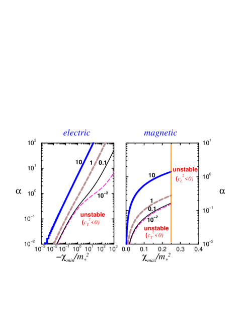
FIG. 2.: Constraints yielding minimum and maximum values for the normalized current $\chi/m_{\ast}^{2}$, according to Eqs. (55), (57), and (58), for values $\lambda q^{2}=10^{-2}$ to $10$. In the figure on the left, for each particular value of $\lambda q^{2}$, the unstable region (where $c_{{}_{\rm T}}^{\,2}<0$) lies below the corresponding curve. The same is true for the figure on the right, but in addition $\chi/m_{\ast}^{2}<1/4$ for otherwise $c_{{}_{\rm L}}^{\,2}<0$.

The first thing to determine in order to plot $\Upsilon_{r}(\ell_{r})$ is whether the current is timelike or spacelike. This is achieved by looking at Eq. (53) which states that the sign of $\chi$, and hence the timelike or spacelike character of the current, is also the sign of $b^{2}-{\cal K}^{2}$. Now Eq. (39), modified to account for (37), shows that the range of variation of ${\cal K}$ is

$$\chi\geq 0\ \ \hbox{(magnetic)}\Longrightarrow\ 1+\lambda q^{2}\leq{\cal K}\leq 2+\lambda q^{2},$$ (59)

and

$$\chi\leq 0\ \ \hbox{(electric)}\Longrightarrow\ \lambda q^{2}\leq{\cal K}\leq 1+\lambda q^{2}.$$ (60)

Therefore, it is only possible for $\chi$ to be positive if $b\geq 1+\lambda q^{2}$, and negative otherwise. So we deal with a magnetic configuration or an electric configuration depending on whether $b$ is respectively greater or less than its critical value $b_{c}=1+\lambda q^{2}$. Since $\chi$ cannot change sign dynamically, by fixing $b$ one also fixes the character of the current and, where the physical constraints (55) to (58) cease to be satisfied, the curves plotted in the various figures end. As the quantity $b_{c}$ was unity in the decoupled case, we see that electromagnetic corrections can modify the nature of the current for a given set of integer numbers $Z$ and $N$.

FIG. 3.: Variations of the self potential $\Upsilon_{r}$ with the ring’s circumference $\ell_{r}$ and the electromagnetic self coupling $\lambda q^{2}$ for $\alpha=b=1$. The thick curve stands for various values of $\lambda q^{2}<0.1$ for which they are undistinguishable, and in the “safe” zone; the minimum value of $\Upsilon_{r}$ is then $M_{v}$, the vorton mass. $\Upsilon_{r}$ for the same parameters $\alpha$ and $b$, this time for $\lambda q^{2}=1$ is represented as the full thin line, where it is clear that we now are in a “dangerous” zone where the potential has a minimum (new value for $M_{v}$) but now terminates at some point where it equals $M_{s}$. Finally the dashed curve represents the potential for $\lambda q^{2}=10$, an unrealistically large value, and this time the curve terminates even before reaching a minimum: this is a “fatal” situation for all loops with such parameters will eventually decay.

Once the nature of the current is fixed, it is a simple matter to evaluate the potential $\Upsilon_{r}$, and it is found, as in Ref. [13], that three cases are possible, depending on the values of the free parameters, namely the so–called “safe”, “dangerous” and “fatal” cases. They correspond to whether the thin string description holds for all values of the allowed parameters or not, as illustrated on Fig. 3.

The general form of the potential $\Upsilon_{r}(\ell_{r})$ exhibits a minimum and two divergences, one at the origin which prevents a collapse of the loop, and one for $\ell_{r}\to\infty$ which holds the loop together and is responsible for the confinement effect [13]. The latter divergence, going like $\Upsilon_{r}\sim\ell_{r}$, occurs whatever the underlying parameters may be and is mainly due to the fact that it requires an infinite amount of energy to enlarge the loop to infinite size, its energy per unit length being bound from below ($U\geq m^{2}$). The divergence at $\ell_{r}=0$ is however not generic, as is shown on Fig. 3, since for some sets of parameters, the quantity $\ell_{r}$ does not take values in its entire range of potential variations $[0,\infty[$. This can be seen as follows.

FIG. 4.: The characteristic behavior of $\ell_{r}$ as a function of $\chi_{r}$ for $\lambda q^{2}=1$ in the magnetic regime where $\chi_{r}>0$: the curve down, indicated $b<\lambda q^{2}+2$ is for $b=2.1$, and the upper curve for $b=5$. They all diverge around $\chi_{r}=0$.

On the magnetic side, the function $\ell_{r}^{2}(\chi_{r})$ ranges from $+\infty$ in the limit where $\chi_{r}\to 0^{+}$, to $4[b^{2}-(\lambda q^{2}+2)^{2}]/(\lambda q^{2}+2)$ for $\chi_{r}\to 1/4$ as sketched on Fig. 4. Depending therefore on whether $b$ is less or greater than $(\lambda q^{2}+2)$, the $\ell_{r}=0$ limit will or will not exist. In the former case, the potential $\Upsilon_{r}$, which diverges for $\ell_{r}\to 0$, will have the form indicated as the thick curve on Fig. 3, and the string loop solution is in a “safe” zone. If $b>\lambda q^{2}+2$, then the minimum value for $\ell_{r}^{2}$ is non zero so the potential terminates at some point, which can be either sufficiently close to the origin that the minimum for $\Upsilon_{r}$ can be reached (“dangerous” zone) or not (“fatal” zone). In the former case, the resulting configuration may reach an equilibrium state of mass $M_{v}$ (when radiation is taken into account, such a configuration will eventually loose enough energy to settle down into a vorton state) provided its mass $M$ is less than that obtained for $\chi_{r}=1/4$, $M_{s}$ say, with the same set of parameters, whereas it will enter a regime in which the thin string description is no longer valid if $M>M_{s}$. Finally, there is also the possibility that no minimum of $\Upsilon_{r}(\ell_{r})$ is attainable on the entire available range for $\ell_{r}$; this is called “fatal” because, whatever the value of $M$, the loop again ends up in the region where no string description holds anymore. When this happens, the topological stability of the vortex can be removed dynamically and the quantum effects make the loop decay into a burst of Higgs particles.

The electric regime presents roughly the same features of having “safe”, “dangerous” and “fatal” zones, although for slightly different reasons: the magnetic case ends either when $c_{{}_{\rm L}}^{\,2}\to 0$ or $c_{{}_{\rm T}}^{\,2}\to 0$ whereas the electric case does so only in the case $c_{{}_{\rm T}}^{\,2}\to 0$. On Fig. 5 is sketched the function $\ell_{r}(\chi_{r})$ for $\chi_{r}<0$ and various values of the parameters $b$, given $\lambda q^{2}$. What happens in the electric regime is that the limiting case this time is for $b=\lambda q^{2}$, $\ell_{r}^{2}$ behaving as $(b^{2}-\lambda^{2}q^{4})/(\lambda^{2}q^{4}\chi_{r})$ as $\chi_{r}\to-\infty$; thus, if $b<\lambda q^{2}$, as $\chi_{r}$ is negative, $\ell_{r}^{2}$ is always non zero and there must exist a value for $\chi_{r}$ such that the string’s tension vanishes, and the loop itself becomes unstable with respect to transverse perturbations. Such a loop would clearly not form a vorton. On the other hand, if $b>\lambda q^{2}$, then $\ell_{r}^{2}$ can get to zero, and for some values of the parameters (unfortunately the range is not derivable analytically), it will do so before the tension vanishes. The corresponding loop might then end as a vorton.

FIG. 5.: The characteristic behavior of $\ell_{r}$ as a function of $\chi_{r}$ for $\lambda q^{2}=1$ in the electric regime where $\chi_{r}<0$: The curve down is for a “safe” configuration with $b=1.9>\lambda q^{2}$, whereas the upper curve is “fatal”, with $b=0.1<\lambda q^{2}$. The two upper curves terminate at the point where the string tension becomes negative and the string is unstable with respect to transverse perturbations.

Finally the safe zone, for all regimes taken together, is limited to

$$\lambda q^{2}\leq b\leq\lambda q^{2}+2,$$ (61)

a condition which is increasingly restrictive as $\lambda q^{2}$ increases, and may even forbid vorton formation altogether for a very large coupling.

VII Conclusions

We have exhibited explicitely the influence of electromagnetic self corrections on the dynamics of a circular vortex line endowed with a current at first order in the coupling between the current and the self–generated electromagnetic field, i.e., neglecting radiation. This is necessary before any radiation can be taken into account and evaluated, a task which is still to be done. Moreover, use of the duality formalism developed by Carter [18] has been made and shown to be especially useful in this particular case in the sense that it enabled us to derive the dynamical properties of a proto–vorton configuration analytically. It is to be expected that such a dual calculation will prove indispensable when evaluation of the higher electromagnetic orders will be performed.

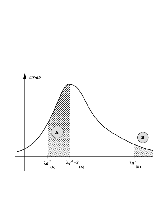
FIG. 6.: A possible way out of the vorton excess problem: a sketch of a distribution of loops with $b$, and “safe” intervals [cf. Eq. (61)] for different values of $\lambda q^{2}$. It is clear that the actual number density of ensuing vortons, at most proportional to the shaded areas, will depend quite strongly on the location of the safety interval. Note also that this electromagnetic correction may reduce drastically the available phase space for vorton formation since the maximum of the $dN/db$ distribution is usually assumed to be peaked around $b=1$.

We have shown that most of the conclusions of our previous paper on that subject actually hold when electromagnetism is accounted for, at least at this order, with the result, perhaps not intuitively obvious from the outset, that this self–interaction tends to destabilise the string loops towards states for which a classical string description does not hold, configurations which are expected to decay into the string constituents (the Higgs field in particular) when quantum effects are taken into account.

As is clear from Eq. (61), increasing the electromagnetic correction is equivalent to reducing the available phase space for vorton formation, as $b$ of order unity is the most natural value [6], situation that we sketch in Fig. 6. On this figure, we have assumed a sharply peaked $dN/db$ distribution centered around $b=1$; with $\lambda q^{2}=0$, the available range for vorton formation lies precisely where the distribution is maximal, whereas for any other value, it is displaced to the right of the distribution. Assuming a gaussian distribution, this effect could easily lead to a reduction of a few orders of magnitude in the resulting vorton density, the latter being proportional to the area below the distribution curve in the allowed interval. This means that as the string loops contract and loose energy in the process, they keep their “quantum numbers” $Z$ and $N$ constant, and some sets of such constants which, had they been decoupled from electromagnetism, would have ended up to equilibrium vorton configurations, instead decay into many Higgs particles, themselves unstable. This may reduce the cosmological vorton excess problem [6] if those are electromagnetically charged.

The present analysis, because of its being restricted to exactly circular configurations, is not sufficient to provide general conclusions as to whether vortons will form or not for whatever original loop shapes, but clearly indicates that even though the cosmological vorton problem [6] cannot be solved by means of this destabilizing effect, it may well have been slightly overestimated.

REFERENCES

- [1] T. W. B. Kibble, J. Phys. A 9, 1387 (1976), Phys. Rep. 67, 183 (1980).
- [2] E. P. S. Shellard & A. Vilenkin, Cosmic strings and other topological defects, Cambridge University Press (1994).
- [3] E. Witten, Nucl. Phys. B 249, 557 (1985).
- [4] R. L. Davis, E. P. S. Shellard, Phys. Rev. D38, 4722 (1988); Nucl. Phys. B 323, 209 (1989);
- [5] B. Carter, Ann. N.Y. Acad.Sci., 647, 758 (1991); B. Carter, Proceedings of the XXXth Rencontres de Moriond, Villard–sur–Ollon, Switzerland, 1995, Edited by B. Guiderdoni and J. Tran Thanh Vân (Editions Frontières, Gif–sur–Yvette, 1995).
- [6] R. Brandenberger, B. Carter, A.–C. Davis, M. Trodden, Phys. Rev. D54, 6059 (1996).
- [7] B. Carter, X. Martin, Ann. Phys. 227, 151 (1993).
- [8] X. Martin, Phys. Rev. D50, 749 (1994).
- [9] P. Peter, Phys. Rev. D45, 1091 (1992).
- [10] P. Peter, Phys. Rev. D46, 3335 (1992).
- [11] X. Martin, P. Peter, Phys. Rev. D51, 4092 (1995).
- [12] A. L. Larsen, M. Axenides, Class. Quantum Grav. 14, 443 (1997)
- [13] B. Carter, P. Peter, A. Gangui, Phys. Rev. D55, 4647 (1997).
- [14] B. Carter, P. Peter, Phys. Rev. D52, R1744 (1995).
- [15] B. Carter, Electromagnetic self–interaction in strings, Phys. Lett. B (1997) in press.
- [16] E. Copeland, D. Haws, M. Hindmarsh, N. Turok, Nucl. Phys. B 306, 908 (1988).
- [17] B. Carter, in Formation and Interactions of Topological Defects (NATO ASI B349), ed R. Brandenberger & A.–C. Davis, pp 303–348 (Plenum, New York, 1995).
- [18] B. Carter, Phys. Lett. B 224, 61 (1989) and B 228, 466 (1989).
- [19] Y. Nambu, Proceedings of Int. Conf. on Symmetries and Quark models, Wayne State University, (1969); T. Goto, Prog. Theor. Phys. 46, 1560 (1971).
- [20] A.L. Larsen, Class. Quantum. Grav. 10, 1541 (1993).
- [21] B. Carter, Phys. Rev. Lett.74, 3093 (1995); X. Martin, Phys. Rev. Lett.74, 3102 (1995).
- [22] A. Babul, T. Piran, D. N. Spergel, Phys. Lett. B 202, 307 (1988).
- [23] P. Peter, J. Phys. A 29, 5125 (1996).
- [24] M. Alford, K. Benson, S. Coleman, J. March–Russell, Nucl. Phys. B 349, 414 (1991).
- [25] P. Peter, Phys. Rev. D46, 3322 (1992)
- [26] B. Carter, Nucl. Phys. B412, 345 (1994)
- [27] B. Carter, V.P. Frolov, O. Heinrich, Class. Quantum. Grav., 8, 135 (1991).
- [28] B. Carter, Class. Quantum. Grav. 9S, 19 (1992).
- [29] B. Carter, Phys. Lett. 238, 166 (1990).