McGill/97-7

hep-ph/9705201

April 30, 1997

Supersymmetric Electroweak Phase Transition:
Dimensional Reduction versus Effective Potential

James M. Cline

McGill University, Montréal, Québec H3A 2T8, Canada

and

Kimmo Kainulainen

High Energy Physics Division,
P.o. Box 9, FIN-00014, University of Helsinki

Abstract

We compare two methods of analyzing the finite-temperature electroweak phase transition in the minimal supersymmetric standard model: the traditional effective potential (EP) approach, and the more recently advocated procedure of dimensional reduction (DR). The latter tries to avoid the infrared instabilities of the former by matching the full theory to an effective theory that has been studied on the lattice. We point out a limitation of DR that caused a large apparent disagreement with the effective potential results in our previous work. We also incorporate wave function renormalization into the EP, which is shown to decrease the strength of the phase transition. In the regions of parameter space where both methods are expected to be valid, they give similar results, except that the EP is significantly more restrictive than DR for the range of baryogenesis-allowed values of $\tan\beta$, $m_{h}$, the critical temperature, and the up-squark mass parameter $m_{U}$. In contrast, the DR results are consistent with $2\mbox{\raisebox{-2.58334pt}{~{}$\stackrel{{\scriptstyle<}}{{\sim}}$~{}}}\tan\beta\mbox{\raisebox{-2.58334pt}{~{}$\stackrel{{\scriptstyle<}}{{\sim}}$~{}}}4$, $m_{h}<80$ GeV, and $m_{U}$ sufficiently large to have universality of the squark soft-breaking masses at the GUT scale, in a small region of parameter space. We suggest that the differences between DR and EP are due to higher-order perturbative corrections rather than infrared effects.

1 Introduction

Recently a new method has been proposed and exploited to try to improve the reliability of analyzing first-order phase transitions in finite-temperature gauge theories, called dimensional reduction (DR) [1]. In the traditional effective potential (EP) approach, a problem is posed by the transverse gauge bosons which are very light, and thus can lead to infrared instabilities in the effective theory. Their effects should in principle be treated nonperturbatively to reliably compute the strength of the transition. Dimensional reduction works around this by integrating out all the heavy modes in a given theory to obtain an effective theory of the problematic light modes, which is then studied on the lattice [2]. This program was carried out in refs. [1, 2] for the standard model. However, the nonperturbative lattice results of ref. [2] are applicable to other theories as well, since the only requirement is that the effective theory after integrating out the heavy fields has the same degrees of freedom as does the standard model, namely the light Higgs doublet and the transverse gauge bosons.

One of the most interesting applications of DR is to supersymmetric (SUSY) models, since these have the possibility of producing the baryon asymmetry of the universe at the electroweak phase transition [3]. In order to preserve the baryons thus created, the phase transition must be strongly enough first order, meaning in this context that the VEV of the Higgs fields must be sufficiently large at the critical temperature:

$$v(T_{c})/T_{c}\equiv(v_{1}^{2}+v_{2}^{2})^{1/2}/T_{c}\mbox{\raisebox{-2.58334pt}{~{}$\stackrel{{\scriptstyle>}}{{\sim}}$~{}}}1-1.5$$ (1)

Otherwise anomalous baryon-violating interactions mediated by electroweak sphalerons will be too fast in the broken phase after the transition, and quickly wash out the baryon asymmetry that was created. The range of values on the right hand side of (1) comes from an estimate of the uncertainty in the sphaleron rate at two loops, and in dynamical details like the amount of reheating in the phase transition [2]. In the DR approach, condition (1) is replaced by the requirement that the ratio of the Higgs quartic coupling to the squared gauge coupling must be small enough in the effective three-dimensional theory,

$$x_{c}\equiv{\lambda_{3}/g_{3}^{2}}<0.026-0.044.$$ (2)

The two quantities are related to each other by lattice measurements of $v(T_{c})/T_{c}$ in ref. [2]; we have used their results to obtain the fit

$$v(T_{c})/T_{c}\simeq 1.087w^{2}-2.916w+2.911;\quad w\equiv x_{c}/0.04,$$ (3)

which is valid in the interval corresponding to (1) and (2).

References [4]-[7] have studied the phase transition in the minimal supersymmetric standard model (MSSM) using DR, identifying the regions in the SUSY parameter space consistent with condition (2). One of the purposes of this letter is to explain the differences between our results [4] and the others [5]-[7]. In the process we shall elucidate a possible shortcoming of DR: even moderately heavy squarks can be too light to reliably integrate out if the superrenormalizable cubic scalar couplings of the MSSM become too large.

More generally we are interested in determining the extent to which the results of dimensional reduction differ from those of the effective potential (EP) approach [8]-[14]. We have therefore undertaken a comparison of the two methods in the MSSM, exploring as broad a region of parameter space as possible. We find that they give results which are in reasonable qualitative agreement. A further goal is to characterize which regions of MSSM parameter space are suitable for electroweak baryogenesis. We have thus recomputed the distributions of MSSM parameters, as well as some observables, that are baryogenesis-compatible. Where comparison is possible, our results agree well with some [5] of the previous DR studies that have focused on more specific regions of parameter space, and less well with others [7].

The dimensional reduction procedure employed here is essentially the same as we used in ref. [4] (hereafter called CK), which includes the one-loop corrections proportional to the top and bottom yukawa couplings, $y_{t,b}$. One must integrate out the third family quarks and squarks at zero and at finite temperature to find the effective finite-$T$ lagrangian and to relate its couplings to physical quantities. The combination $\lambda_{3}/g_{3}^{2}$ in eq. (2) can thus be expressed a function of squark masses and mixing angles, Higgs boson masses and $\tan\beta$, allowing one to infer from the inequality (2) which are the baryogenesis-compatible regions in the space of physical parameters.

2 Dimensional reduction: subleading corrections

Because $x_{c}$ needs to be small for purposes of baryogenesis, we are interested in cases where there are large cancellations between the tree-level and one-loop contributions to $\lambda_{3}$. For quantitative accuracy it therefore appears important to include some formally subleading contributions in the finite-$T$ effective lagrangian, which were omitted in CK. Among the potentially most important such terms are those due to thermal loops of gauge and Higgs bosons, which shift the Higgs boson mass terms [5] by an amount

$$\delta{\cal L}_{3}/T=\left(\frac{1}{4}g^{2}T^{2}+\frac{3g^{2}}{16\pi}Tm_{A_{0}}\right)(|H_{1}|^{2}+|H_{2}|^{2}),$$ (4)

where

$$m^{2}_{A_{0}}=\frac{5}{2}g^{2}T^{2}+\frac{g^{2}}{8\pi^{2}}(3m^{2}_{Q}+m_{A}^{2})).$$ (5)

These additional terms lower the estimate of the critical temperature from that found in CK; they alone can increase the final value of the parameter $x_{c}$ by $\sim 0.008$. However, there is also another, direct contribution to $x_{c}$ from the same particles,

$$\delta x_{g}=\frac{g^{2}\ln 2}{32\pi^{2}}\cos^{2}\!2\alpha-\frac{3g^{2}T}{128\pi m_{A_{0}}},$$ (6)

where the angle $\alpha$ defines the direction of the phase transition in the $(H_{1},H_{2})$-plane. Both in (4) and (6) the first term comes from superheavy (nonzero Matsubara frequency) and the second from heavy scale (zero Matsubara frequency) integration. The correction (6) is $\sim-0.003$, partly cancelling the effect on $x_{c}$ from the thermal self-energies in (4); we argue that this combined effect of $\sim 0.005$ is the typical scale of dominant $g^{2}$-corrections.

Taking into account these improvements, our full result for $x_{c}$ can be written as

$$x_{c} = {g^{2}+g^{\prime 2}\over 8g^{2}}\cos^{2}\!2\alpha$$ (7)

$$+ {3\ln 2\over 4\pi^{2}}\left({y_{t}^{4}\over g^{2}}\sin^{4}\!\alpha-\frac{g^{2}+g^{\prime 2}}{4g^{2}}y_{t}^{2}\cos 2\alpha\sin^{2}\!\alpha\right)$$

$$- \frac{y^{2}_{t}(g^{2}+g^{\prime 2})}{4g^{2}}\,\left(\frac{\zeta(3)}{12\pi^{4}T^{2}}+\frac{T}{4\pi M^{3}_{D_{t}}}\right)\left(\mu^{2}\cos^{2}\!\alpha-A^{2}_{t}\sin^{2}\!\alpha\right)\cos 2\alpha$$

$$+ \left(t\leftrightarrow b;\,\cos\alpha\leftrightarrow\sin\alpha\right),{}$$

$$+ \delta x^{SH}+\delta x^{H}+\delta x_{g}$$

Here $M_{D_{t}}$ is the sum of the Debye masses left- and right-handed top squarks [4],

$$M_{D_{t}}=m_{\tilde{t}_{L}}+m_{\tilde{t}_{R}},$$ (8)

and the thermal corrections are computed assuming the gauginos and higgsinos are decoupled. The first three lines in (7) are, respectively, the contributions from tree-level, leading superheavy scale, and the superheavy and heavy scale wave function renormalizations. The fourth line shows how to obtain the effect of the bottom sector from that of the top (notice that the interchange of $\sin\alpha$ and $\cos\alpha$ implies $\cos 2\alpha\to-\cos 2\alpha$). The last line gives the next-to-leading superheavy scale shift $\delta x^{SH}$, the much larger term $\delta x^{H}$ from the same Feynman diagrams in the heavy scale integration, and the gauge boson term from (6). The additional function $\delta x^{SH}$ is given by

$$\delta x^{SH} = \frac{1}{g^{2}}\biggl{(}-\frac{3}{2}y_{t}^{4}\sin^{2}\!\alpha\sum_{a=Q,U}\left(\sin^{2}\!\alpha f^{SH}_{2}(m_{a},m_{a})-2S^{t}_{a}f^{SH}_{3}(m_{Q},m_{a},m_{U})\right){}$$ (9)

$$\phantom{HH}-\frac{3}{2}y_{t}^{4}(S^{t}_{a})^{2}f^{SH}_{4}(m_{Q},m_{Q},m_{U},m_{U})-\frac{3}{2}g^{2}y_{t}^{2}F^{SH}_{\alpha}(m_{Q},m_{U})\;\cos 2\alpha{}$$

$$\phantom{Han}+\left(t\leftrightarrow b;\;U\leftrightarrow D;\;\sin\alpha\leftrightarrow\cos\alpha\right)\biggr{)}{}$$

$$+\frac{g^{\prime 2}}{4g^{2}}\biggl{(}y_{t}^{4}(F^{SH}_{\alpha}(m_{Q},m_{U})-4F^{SH}_{\alpha}(m_{U},m_{Q})){}$$

$$\phantom{+l\frac{g}{4}}+y_{b}^{4}(F^{SH}_{\alpha}(m_{Q},m_{D})+2F^{SH}_{\alpha}(m_{D},m_{Q}))\biggr{)}\cos 2\alpha$$

with $F^{SH}_{\alpha}(m_{a},m_{b})\equiv\sin^{2}\!\alpha f^{SH}_{2}(m_{a},m_{a})-S^{t}_{\alpha}f^{SH}_{3}(m_{a},m_{a},m_{b})$, $S^{t}_{\alpha}\equiv(\mu\cos\alpha+A_{t}\sin\alpha)^{2}$. The high-temperature expansions of the $n$-point loop integrals $f^{SH}_{n}$ (following the notation of [5]) are

$$f^{SH}_{2}(m_{a},m_{a}) \simeq -\frac{\zeta(3)}{64\pi^{4}}\frac{m_{a}^{2}}{T^{2}}{}$$

$$f^{SH}_{3}(m_{a},m_{a},m_{b}) \simeq \frac{\zeta(3)}{128\pi^{4}T^{2}}-\frac{\zeta(5)}{128\pi^{6}}\frac{2m_{a}^{2}+m_{b}^{2}}{T^{4}}{}$$

$$f^{SH}_{4}(m_{a},m_{a},m_{b},m_{b}) \simeq \frac{\zeta(5)}{1024\pi^{6}T^{4}}$$ (10)

to leading order in $m^{2}/T^{2}$. The contribution from the heavy scale, $\delta x^{H}$, has the same form as $\delta x^{SH}$; one merely replaces the masses $m_{Q,U,D}$ by the corresponding Debye masses (see ref. [4]) and the integrals (10) by their heavy scale counterparts, which are exactly given by

$$f^{H}_{2}(m_{a},m_{a}) = \frac{T}{8\pi m_{a}}{}$$

$$f^{H}_{3}(m_{a},m_{a},m_{b}) = \frac{T}{8\pi m_{a}(m_{a}+m_{b})^{2}}{}$$

$$f^{H}_{4}(m_{a},m_{a},m_{b},m_{b}) = \frac{T}{8\pi m_{a}m_{b}(m_{a}+m_{b})^{3}}.$$ (11)

In CK we omitted $\delta x^{HS}$ and the corresponding corrections to the wave function renormalization, since they are formally subleading. The combined effect of all the new terms we consider here is an increase in $x_{c}$ of varying size, but never larger than $0.015$.

3 Constraint on superrenormalizable couplings

Despite the significance of the subleading contributions which we now take into account, the most important difference between this work and CK is that we have imposed a consistency condition on the size of the $\mu$ and $A_{t,b}$ parameters of the MSSM, the necessity of which was not recognized previously. These couplings are distinguished by the fact that they appear in superrenormalizable interactions among the squark and Higgs bosons in the MSSM Lagrangian:

$${\cal L}_{\rm{\scriptscriptstyle}MSSM}=y_{t}\,\tilde{t}_{L}^{*}(\mu H_{1}+A_{t}H_{2})\tilde{t}_{R}+y_{b}\,\tilde{b}_{L}^{*}(\mu H_{2}+A_{b}H_{1})\tilde{b}_{R}+\cdots$$ (12)

Because of their dimensionality, one must be especially vigilant against the breakdown of the heavy scale perturbative expansion due to large infrared contributions to the three-dimensional finite-$T$ effective Lagrangian (where the effective quartic coupling has dimensions of $T$), of order

$$\delta\lambda_{3}\sim{y^{2}_{t}T\over 16\pi M^{4}_{D_{t}}}|\mu H_{1}+A_{t}H_{2}|^{4},$$ (13)

coming from diagrams like figure 1. In the present study we have imposed an upper limit on the ratio of $\mu$ and $A_{t,b}$ to $M_{D_{t,b}}$ to safeguard against such a breakdown. Precisely, we required that

$$\frac{|\mu|}{M_{D_{t,b}}},\,\frac{|A_{t,b}|}{M_{D_{t,b}}}<1;\ \hbox{and}\ |\mu|,|A_{t,b}|<500\ \hbox{GeV}.$$ (14)

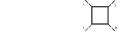
Figure 1: A contribution to the effective quartic coupling of Higgs bosons involving the interactions of eq. (12), and generating the term (13) in the effective Lagrangian. At finite temperature it is infrared divergent if the masses of the squarks in the loop vanish.

The precise values chosen for the bounds (14) are somewhat arbitrary. However the region of MSSM parameter space that satisfies the sphaleron bound but violates (14) appears to be an isolated “island” which, once excluded by (14), is not further reduced by making (14) more stringent. These new consistency conditions make a dramatic change in the regions of MSSM parameter space which are most likely to give a strong phase transition, and are the main reason for the differences between the present results and those in CK. There our baryogenesis-allowed points were dominated by surprisingly high critical temperatures near 300 GeV. We have subsequently investigated such large-$T_{c}$ points using the EP and found that for them, $v/T$ falls below 1 very rapidly with a slight increase in $T$. Since the present estimate of $T_{c}$ (the temperature where the second derivative of the potential at zero field has vanishing determinant) is already an underestimate of the true $T_{c}$ (where there are degenerate minima of the potential), such behavior means that the transition is quite unlikely to be strongly enough first order for baryogenesis. We find a clear separation between these spurious solutions to the sphaleron bound, and the acceptable ones with $T_{c}$ near 100 GeV, on which we focus henceforth.

The conditions (14) also constitute an important difference between DR and EP. In EP the constraints (14) are not needed, unless one made an expansion of the field-dependent mass eigenvalues of the squarks in powers of $A_{t}$ and $\mu$. But since EP uses the exact field-dependent tree-level squark masses, it resums what would be an infinite series of nonrenormalizable contributions to the effective theory. In DR on the other hand, one must match the parameters of the effective theory onto the renormalizable Lagrangian that has been studied on the lattice. We therefore have no choice but to truncate the effective theory at the order of the renormalizable operators. To improve upon this, it will be necessary to simulate the full MSSM on the lattice, but in the meantime EP is the only method which has a hope of reliably determining the strength of the phase transition for values of $\mu$ and $A_{t}$ where (14) does not hold.

4 The effective potential

To compare DR to the effective potential approach, we constructed the EP at the one-loop, ring-improved level, including contributions of the virtual standard model particles plus the top and bottom quarks and squarks, and the Higgs bosons. This extends the work described in ref. [9] where the bottom sector and Higgs bosons were omitted. We find that the inclusion of the bottom squarks shifts the critical temperature significantly ($10-20$%), but has a small effect on $v/T$, for experimentally allowed values of the lightest Higgs boson mass. After successfully reproducing the results of ref. [9], we further improved the EP by supplementing it with the same wave function renormalization as we computed in the DR approach. Usually wave function renormalization is ignored in the EP, and the one-loop, ring-improved effective lagrangian for the Higgs fields is taken to be

$${\cal L}_{\rm eff} = \sum_{i}|D_{\mu}H_{i}|^{2}-V_{\rm tree}(H_{i})+\frac{1}{64\pi^{2}}{\rm Str}\,M^{4}(H_{i})\left(\ln{M^{2}(H_{i})\over Q^{2}}-\frac{3}{2}\right)$$ (15)

$$+ {\rm Str}\,T\!\int{d^{3}p\over(2\pi)^{3}}\ln\left(1\pm e^{-\sqrt{p^{2}+M^{2}(H_{i})}}\right)-\frac{T}{12\pi}{\rm Tr}(M_{D}^{3}(H_{i},T)-M^{3}(H_{i})).$$

Here Str denotes the supertrace, $\pm$ is $+(-)$ for fermions (bosons), Tr is the trace over bosons only, $m_{D}$ is the thermally corrected Debye mass, and $Q$ is the renormalization scale. However it is more accurate to also include the renormalization of the kinetic term so that $\sum_{i}|D_{\mu}H_{i}|^{2}$ becomes $\sum_{ij}Z_{ij}(D_{\mu}H_{i})^{\dagger}D_{\mu}H_{j}$. After rescaling the fields to canonical form and ignoring effects of two-loop order, this amounts to making the replacement

$$V_{\rm tree}(H_{i})\to V_{\rm tree}(\sum_{j}Z^{-1}_{ij}H_{j}).$$ (16)

One reason for making this improvement is to try to minimize any possible sources of discrepancies between DR and EP. We find that including wave function renormalization reduces the strength of the phase transition noticeably, though not drastically. The comparison is shown in figure 2, where we have plotted contours of $v(T_{c})/T_{c}$ in the plane of $\tan\beta$ and $m_{A}$ (the pseudoscalar Higgs boson mass), for $m_{t}=170$ GeV, $m_{Q}=280$ GeV, $m_{U}=0$, $A_{t}=\mu=0$.

To include the effects of the Higgs bosons in the EP, we used the following for the field-dependent parts of the mass matrices for the CP-even, CP-odd and charged bosons, respectively:

$$M^{2}_{H}(H_{i}) = M^{2}_{H}(0)+\frac{T^{2}}{4}\left(\begin{array}[]{cc}3y_{b}^{2}+g^{2}&0\\ 0&3y_{t}^{2}+g^{2}\end{array}\right)+\frac{g^{2}}{4}\left\{\left(\begin{array}[]{cc}3H_{1}^{2}-H_{2}^{2}&-2H_{1}H_{2}\\ -2H_{1}H_{2}&3H_{2}^{2}-H_{1}^{2}\end{array}\right),\right.$$ (26)

$$\left.\left(\begin{array}[]{cc}H_{1}^{2}-H_{2}^{2}&0\\ 0&H_{2}^{2}-H_{1}^{2}\end{array}\right),\quad\hbox{or}\quad\left(\begin{array}[]{cc}H_{1}^{2}+H_{2}^{2}&4H_{1}H_{2}\\ 4H_{1}H_{2}&H_{2}^{2}+H_{1}^{2}\end{array}\right)\right\}.$$

Figure 2: Comparison of the usual effective potential results for the phase transition in the MSSM, to the EP supplemented by wave function renormalization. Heavy convex lines: contours of constant $v/T$ at the critical temperature, in the $\tan\beta$-$m_{A}$ plane. Heavy concave line: contour for $m_{h}=65$ GeV. Light concave lines: contours for other values of $m_{h}$. Fig. 2a is without wave function renormalization, and 2b is with w.f.r. The values of the other MSSM parameters are $m_{t}=170$ GeV, $m_{Q}=280$ GeV, $m_{U}=0$, $A_{t}=\mu=0$.

5 The high-temperature expansion

To obtain the above results for the EP, we used the exact expressions for the $T$-dependent part, without expanding in masses over temperature. In contrast, DR is explicitly a high temperature limit, requiring us to impose the important restriction

$$m_{\tilde{q}_{X}}/T<\pi$$ (27)

on the parameters considered, where $m_{\tilde{q}_{X}}$ is the thermal (Debye) mass of any of the squarks included in the loop corrections, $\tilde{q}_{X}=\tilde{t}_{L,R},\tilde{b}_{L,R}$ [4]. One might therefore naively conclude that EP is valid for a larger range of parameters than is DR. However we wish to argue that one should also make the same restriction (27) to obtain reliable results from the EP, because the ring resummation assumes that all the modes in the “soft” loop (heavy scale) can be taken approximately massless, compared to the modes in the “hard” loops (superheavy scale). Thus the ring-corrected EP is strictly speaking, and somewhat contrary to common wisdom, valid only in high-$T$ limit. Since the EP has the qualitatively correct decoupling limit, when one employs the nonexpanded integral expressions for loop-corrections however, one might hope that the infinite resummation retains some of the qualitative physical features of the exact theory, even outside its region of strict validity. Nevertheless, in what follows we will impose (27) equally on DR and EP.

At the same time however, we cannot allow any of the particles we are integrating out to become arbitrarily light compared to $T$, because this would give rise to infrared divergences, as discussed above, and necessitate a new lattice study with the light fields included in the low-energy lagrangian. Thus we imposed the further constraint

$$\frac{T}{m_{\tilde{q}_{X}}}<1;\qquad\tilde{q}_{X}=\tilde{t}_{L,R},\ \tilde{b}_{L,R}.$$ (28)

This ratio appears as an explicit expansion parameter when integrating out the heavy-scale degrees of freedom; it is the exact analog of the expansion parameter $gT/M_{W}$ in the gauge sector, which at small $M_{W}\sim g\phi$ induced us to use DR rather than EP in the first place. We found that EP is quite sensitive to the exact value taken as the upper limit in (28): using a value of 1 removes 80% of otherwise acceptable parameter sets, whereas using 1.2 leaves essentially all of them. In the present work we imposed (28) only on DR, not on EP.

6 Monte Carlo search of the parameter space

We undertook a Monte Carlo sweep of the MSSM using both methods, DR and EP, to find those parameters allowed by the baryogenesis requirement (1) or (2)

$$x_{c}<0.044\qquad\Leftrightarrow\qquad v(T_{c})/T_{c}>1.0,$$ (29)

and also the bound on the $\rho$ parameter, which we took to be $\Delta\rho<0.011$ as the contribution from the third generation quarks and squarks. It can be seen below that the scarcity of solutions to (29) depends strongly on small changes ($\sim 0.001$) in the value of this upper bound, so that future improvements on the $\rho$ parameter constraint might severely limit the possibilities for electroweak baryogenesis in the MSSM. As in CK, the randomly-varied independent parameters were $\tan\beta$, $m_{t}$, the pseudoscalar mass $m_{A}$, the $\mu$ parameter, and the soft SUSY-breaking parameters $m_{Q}$, $m_{U}$, $m_{D}$, $A_{t}$ and $A_{b}$. The derived quantities are the physical masses of the squarks and lightest Higgs boson, the critical temperature $T_{c}$, $\Delta\rho$, and $v/T$ or $x_{c}$. To compare results, we have converted $x_{c}$ into the equivalent $v/T$ value using eq. (3). To determine $v/T$ with the EP, we numerically solved for the global minimum of the potential, but found that for the parameters of interest this was never more than 1% from the value obtained by minimizing the one-dimensional slice of the potential in the symmetry-breaking direction determined at the origin.

The resulting distributions of parameters are shown in figure 3, where one sees reasonable qualitative agreement between the two methods. However there are several noticeable differences. The maximum allowed up-squark mass parameter is 160 GeV in DR and only 90 GeV in the EP. The largest allowed values of $m_{h^{0}}$, the mass of the lightest Higgs boson, are 84 GeV and 70 GeV respectively. In EP we find a somewhat lower critical temperature (99 GeV versus 92 GeV), and the distribution of $T_{c}$ values is also much narrower there than in DR. The narrowness of the $\tan\beta$ distribution in EP relative to DR has the anticipated correlation with that of $m_{h^{0}}$ since the latter increases in the MSSM with larger $\tan\beta$. Finally one sees also that DR has a broader distribution of $v/T$ than does EP. The fact that DR has less difficulty than EP to satisfy the sphaleron constraint is evident in all the parameter distributions where a difference is discernible.

As for why DR and EP do not agree exactly, we note that the perturbative expansions are somewhat different in the two approaches. In particular the ring-improvement in EP is effectively a nonanalytic resummation with regard to the scalar field dependent terms. The DR counterpart of this is the heavy scale integration with the SH-scale corrected particle (Debye) masses, which is only done to the order of renormalizable terms in the lagrangian. Therefore the two methods differ by contributions that are of two-loop order, and also by nonrenormalizable terms; we believe these are the source of the discrepancies. It is already known that in EP the two-loop contributions may considerably strengthen the order of the transition [12, 14], extending the allowed values in $\tan\beta$ up to $\sim 4$, just as we are now finding in DR but at only one loop. There may be significant higher-order corrections to DR as well. Although we imposed the constraint (28), to ensure the overall convergence of the heavy-scale perturbtion expansion, the two-loop correction may be sizeable when $m_{U}$ is small. Indeed one may roughly estimate that $\delta x_{\rm c,2-loop}\sim(y_{t}^{2}/4\pi)^{2}(T/m_{\tilde{t}_{L}})^{2}\mbox{\raisebox{-2.58334pt}{~{}$\stackrel{{\scriptstyle<}}{{\sim}}$~{}}}0.01$.

Figure 3: Distributions of MSSM parameters satisfying the baryogenesis constraint in the dimensional reduction approach (DR) and in the effective potential approach (EP). Masses are in units of 100 GeV.

7 How small must $m_{U}$ be?

One might wonder how much fine tuning of parameters is needed to make the phase transition strongly first order. One simple assumption is that all the soft-breaking masses are equal at the GUT scale, $m_{Q}=m_{U}=m_{D}$, and therefore only differ from each other at the weak scale by logarithmic corrections. Using the renormalization group equations to run the soft-breaking masses down from their universal GUT-scale value [16], and keeping only the corrections due to the large top quark Yukawa coupling, one can estimate that at the weak scale

$${m_{U}\over m_{Q}}=\left({M_{{\scriptscriptstyle}\rm GUT}\over M_{\rm weak}}\right)^{-y_{t}^{2}/16\pi^{2}}\sim 0.7-0.8,$$ (30)

using $y^{2}_{t}=1.25$ (corresponding to $\tan\beta=2$) and $M_{{\scriptscriptstyle}\rm GUT}=10^{14}-10^{16}$ GeV.

It is encouraging that this goes in the right direction to be consistent with electroweak baryogenesis, since the first order phase transition requires small values of $m_{U}$. However the values of ${m_{U}/m_{Q}}$ derived from the EP tend to be smaller than this: the maximum is 0.8, and values greater than 0.4 are unlikely. In DR, ${m_{U}/m_{Q}}$ has a somewhat less restricted range, going up to 1.6. Although values as large as in (30) are relatively unlikely, at least from the point of view of the parameter space for the MSSM unconstrained by GUT relations, they are nevertheless possible. The distributions for ${m_{U}/m_{Q}}$ in DR and EP are shown in figure 4 (the full extent of the tails of these distributions is not shown). Out of 12,500 accepted points in the DR Monte Carlo, about 200 satisfy (30). Among these points, the two top squarks are typically split by less than 80 GeV with $190<m_{\tilde{t}_{+}}<280$ GeV , the pseudoscalar Higgs boson is heavier than $m_{A^{0}}>180$ GeV, and the right-handed top squark mass parameter lies in the range $60$ GeV $<m_{U}<150$ GeV. For these points $\mu$ and $A_{t}$ can be several hundred GeV but they conspire to give a small value of $\mu+A_{t}\tan\beta$ so that the top squark splitting is small. This region can have a Higgs boson as heavy as $m_{h}=79$ GeV.

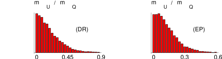
Figure 4: Distributions for ${m_{U}/m_{Q}}$ in DR and EP.

8 Correlations between parameters

In our previous work (CK), there was a strong correlation between the allowed values of $\tan\beta$ and $m_{A}$, including points with arbitrarily large values of $\tan\beta$. These points were all associated with large $T_{c}$, or equivalently with all SUSY breaking parameters at the TeV scale, as discussed above. Constraints (14 and 28) remove all these points from our sample and we find the weaker correlation shown in fig. 5a. The correlation between large $\tan\beta$ and small $m_{U}$ in figure 5b suggests that the failure of EP to allow large $\tan\beta$ may be due to the effects of having a very small value of $m_{U}$.

Figure 5: (a) Baryogenesis-allowed region of MSSM parameter space in DR, projected on (a) the plane of $m_{A^{0}}$ versus $\tan\beta$ and (b) in $m_{U}$ versus $\tan\beta$.

Previous studies of the phase transition in the MSSM have emphasized that large values of the $\mu$ and $A_{t}$ parameters have the effect of weakening the transition. While this may be true while holding all other parameters fixed, if they are instead allowed to vary, one can still find values where the transition is strong even for large $\mu$ and $A_{t}$. Despite the restriction (14) on $\mu$ and $A_{t,b}$ that was used to obtain the present results, fig. 6a shows that a large fraction of the $\mu-A_{t}$ plane is nevertheless represented. This is worth emphasizing because in the MSSM the CP-violating phases which are needed for electroweak baryogenesis are in precisely these parameters. Therefore the regions with larger rather than smaller values of $|\mu|$ or $|A_{t}|$ are the more interesting ones.

Figure 6: Baryogenesis-allowed region of MSSM parameter space in DR, projected on the plane of (a) $\mu$ versus $A_{t}$, and subject to the conditions (14-28), and (b) on the plane of $\Delta\rho$ versus $m_{h}$.

It was mentioned above that the $\rho$ parameter places a stringent constraint on baryogenesis in the MSSM. One finds that it is strongly correlated with various other parameters; in figure 6b we show how in DR it appears to be a limiting factor on how large the lightest Higgs boson mass $m_{h}$ can be. The shape of the correlation between $\Delta\rho$ and $\tan\beta$ looks quite similar, as one might expect from the tree-level formula $m^{2}_{h}=\frac{1}{2}(m^{2}_{A}+m^{2}_{Z}-\sqrt{(m^{2}_{A}+m^{2}_{Z})^{2}-4m^{2}_{A}m^{2}_{Z}\cos^{2}\!2\beta})$: it vanishes at $\tan\beta=1$ and increases for larger $\tan\beta$.

9 Comparison with other DR results

In addition to comparing our DR results with the EP, we have also compared to other published DR results. We have analytically checked that our results agree with those of ref. [5], up to different ways of handling the renormalization procedures (which are two-loop effects), our keeping the finite $g^{\prime}$ effects in the loops, and some numerically small additional terms included in ref. [5]. Numerically our results agree typically to within less than $0.01$ in $x_{c}=\lambda_{3}/g_{3}^{2}$.

More recently, ref. [7] gave results which indicated larger values of the critical ratio $x_{c}$ than did ours, hence a weaker phase transition, for given MSSM parameters. The authors of ref. [7] identified the following possible source for the discrepancy: the direction of symmetry breaking in the plane of the two Higgs fields is very sensitive to the critical temperature $T_{c}$ for small pseudoscalar mass $m_{A}$; a large change in this mixing angle can on the other hand cause large variations in $x_{c}$. We have confirmed this expectation by observing that the tree-level value of $\tan\beta$ (used by ref. [7]) and the one-loop value (used by us) differ significantly for small values of $m_{A}$. Indeed, we find the region of $m_{A}<100$ GeV to be that where the results of all three groups agree least well. Fortunately this region is not particularly essential for baryogenesis, nor for our present results.

The above observation does not fully explain our disagreement with ref. [7] in the large $m_{A}$ region. In fig. 7 we show $x_{c}$ as a function of $m_{A}$ at $\tan\beta=1.75$, for comparison with fig. 2 of [7]. For large $m_{A}$ our asymptotic value of $x_{c}\cong 0.03$ is smaller than theirs by $0.02$. Of this discrepancy, $0.004$ is due to the different definitions of $\tan\beta$. We have also studied the effects of loop contributions of order $g^{2}$ to the Higgs boson mass parameters, neglected by us but included by the authors of [7], and find that they can give a further increase of $0.005$. We are unable to account for the remaining difference of $0.01$.

Figure 7: Critical ratio $x_{c}$ as a function of $m_{A}$ for $\tan\beta=1.75$, showing the dependence on corrections of order $g^{2}$. Other parameters are $m_{Q}=265$ Gev and $m_{U}=100$ GeV, $\mu=A_{t}=0$.

One should bear in mind that the natural scale of the leading terms contributing to $x_{c}$ are of the order of $\sim 0.2$ and the accepted solutions always correspond to a large degree of cancellation between these leading contributions. From this perspective we thus have in fact a rather good numerical agreement with a relative accuracy of about 10 per cent with the other published works in the field. Fig. 7 gives an indication of the sensitivity of $x_{c}$ to the various approximations: omitting all $g^{2}$ corrections, as in CK, putting in the leading $g^{2}$ terms but not $g^{\prime 2}$, and including all the corrections described in this work. The difference between our present work and CK comes dominantly from the neglected squark sector correction $\delta x^{SH}$, equation (9).

There are several effects that make it difficult to achieve a better agreement at this level of approximation. For example we find that differences in the definition of heavy scale squark Debye masses introduce changes of order $0.005$ in $x_{c}$. For both DR and EP we have consistently used the leading order approximations for Debye masses, whereas one could include also the next-to-leading corrections. In the absence of the $T=0$ renormalization of the squark sector this would introduce dependence on the renormalization scale [5], so to get more accurate results the complete renormalization of squark sector at one loop would be required. Also, while the other authors were working in the approximation $g^{\prime}=0$ for the loop corrections, we did not; this too makes differences of order $\sim 0.005$ in $x_{c}$. Finally, different renormalization procedures cause the definitions of $m_{h}$ to differ by terms of two-loop order. If one uses the physical Higgs boson mass as an input instead of $\tan\beta$, getting an accuracy of $0.005$ in $x_{c}$ would require using the two-loop computation for $m_{h}$, since we have checked that a difference of 2-3 GeV in $m_{h}$ changes the corresponding value of $x_{c}$ by $0.005$.

10 Conclusions

In summary, we have compared the one-loop dimensional reduction and the effective potential approaches throughout the parameter space of the MSSM, and found that they give qualitatively similar results for the strength of the electroweak phase transition, although they differ in certain quantitative respects, which should be further explored. We showed that wave function renormalization has a noticeable weakening effect on the phase transition when incorporated into the EP. One potentially interesting difference is that DR appears to allow a smaller hierarchy between the soft-supersymmetry-breaking top squark mass parameters $m_{U}$ and $m_{Q}$, which could make SUSY electroweak baryogenesis compatible with universality at the GUT scale, $m_{U}=m_{Q}$. The top squarks need not have a very large splitting in this case. We have also shown that (in either of the methods used) the phase transition is not necessarily suppressed by large values of $A_{t}$ and $\mu$, which is encouraging since they are likely to be the sources of CP violation if electroweak baryogenesis indeed occurs in the MSSM.

It seems clear that the two-loop corrections are more relevant for accurate results in the MSSM than for the standard model. We leave it for future investigation to see how the differences between DR and EP are affected when one includes the most important two-loop corrections in DR, some of which have recently been incorporated into EP in references [12] and [14]. A further shortcoming in the present state of calculations is that the DR method is no longer applicable in the MSSM if the $\mu$ or $A_{t}$ parameters should be larger than several hundred GeV, or if the top squark becomes too light during the phase transition. While the latter could eventually be accounted for in 3D lattice simulations by including the light squark field in the effective action, to explore the possibility of very large $A_{t}$ or $\mu$ would require a simulation with the full 4D-theory. Let us finally point out, in favour of the DR approach, that for reliable computation of the phase transition dynamics one needs to know not just the order parameter $v(T)/T$, but also other quanitites like the latent heat and surface tension, which are not well-approximated by the EP approach in the standard model [2].

References

- [1] K. Kajantie, M. Laine, K. Rummukainen and M.E. Shaposhnikov, Nucl. Phys. B458 (1996) 90, hep-ph/9508379.
- [2] K. Kajantie, M. Laine, K. Rummukainen and M.E. Shaposnikov, Nucl. Phys. B466 (1996) 189, hep-lat/9510020.
-
[3]
P. Huet and A. Nelson, Phys. Rev. D53, 4578 (1996);
M. Aoki, N. Oshimo and A. Sugamoto, preprint OCHA-PP-87, hep-ph/961225 (1996);
M. Carena, M. Quiros, A. Riotto, I. Vilja, and C.E.M. Wagner, preprint CERN-TH-96-242, hep-ph/9702409 (1997);
M.P. Worah,, preprint SLAC-PUB-7417, hep-ph/9702423 (1997). - [4] J.M. Cline and K. Kainulainen, Nucl. Phys. B482 (1997) 73, hep-ph/9605235.
- [5] M. Laine, Nucl. Phys. B481 (1996) 43, hep-ph/9605283.
- [6] M. Losada, Rutgers preprint RU-96-25, hep-ph/9605235 (1996); hep-ph/9612337 (1996).
- [7] G. Farrar and M. Losada, Rutgers preprint RU-96-26, hep-ph/9612346 (1996).
- [8] J. Espinosa, M. Quiros and F. Zwirner, Phys. Lett. B307 (1993) 106.
- [9] A. Brignole, J. Espinosa, M. Quiros and F. Zwirner, Phys. Lett. B324 (1994) 181.
- [10] M. Carena, M. Quiros, C.E.M. Wagner, Phys. Lett. B380 (1996), hep-ph 9603420.
- [11] D. Delepine, J.-M. Gérard, R. Gonzalez Felipe and J. Weyers, Phys. Lett. B386 (1996) 183, hep-ph/9604440.
- [12] J.R. Espinosa, Nucl. Phys. B475 (1996) 273, hep-ph/9604320 (1996).
- [13] D. Bodeker, P. John, M. Laine and M.G. Schmidt, Heidelberg preprint HD-THEP-96-56, hep-ph/9612364 (1996).
- [14] B. de Carlos and J.R. Espinosa, Sussex preprint SUSX-TH-97-005, hep-ph/9703212 (1997).
- [15] A. Kusenko, P. Langacker and G. Segre, Phys. Rev. D54 (1996) 5824, hep-ph/9602414.
- [16] A.B. Lahanas and K. Tamvakis Phys. Lett. B348 (1995) 451-456, hep-ph/9412281.