CERN-TH/97-81

BI-TP 97/10

HD-THEP-97-17

hep-ph/9704416

April 28, 1997

{centering}

3D SU($N$) + ADJOINT HIGGS THEORY AND
FINITE TEMPERATURE QCD

K. Kajantiea,b111keijo.kajantie@cern.ch, M. Lainec222m.laine@thphys.uni-heidelberg.de, K. Rummukainend333kari@physik.uni-bielefeld.de and M. Shaposhnikova444mshaposh@nxth04.cern.ch

aTheory Division, CERN, CH-1211 Geneva 23, Switzerland
bDepartment of Physics, P.O.Box 9, 00014 University of Helsinki, Finland
cInstitut fΓΌr Theoretische Physik, Philosophenweg 16,
D-69120 Heidelberg, Germany
dFakultΓ€t fΓΌr Physik, Postfach 100131, D-33501 Bielefeld, Germany

Abstract

We study to what extent the three-dimensional SU($N$) + adjoint Higgs theory can be used as an effective theory for finite temperature SU($N$) gauge theory, with $N=2,3$. The parameters of the 3d theory are computed in 2-loop perturbation theory in terms of $T/\Lambda_{\overline{\rm MS}},N,N_{f}$. The perturbative effective potential of the 3d theory is computed to two loops for $N=2$. While the Z($N$) symmetry probably driving the 4d confinement-deconfinement phase transition (for $N_{f}=0$) is not explicit in the effective Lagrangian, it is partly reinstated by radiative effects in the 3d theory. Lattice simulations in the 3d theory are carried out for $N=2$, and the static screening masses relevant for the high-temperature phase of the 4d theory are measured. In particular, we measure non-perturbatively the $O(g^{2}T)$ correction to the Debye screening mass. We find that non-perturbative effects are much larger in the SU(2) + adjoint Higgs theory than in the SU(2) + fundamental Higgs theory.

1 Introduction

Corresponding to the known forces of nature there are two important finite temperature phase transitions in elementary particle matter: the QCD phase transition at $T=O(100)$ MeV and the EW (electroweak) phase transition at $T=O(100)$ GeV. The former has been studied intensely with numerical lattice Monte Carlo simulations [1] but, due to the difficulties associated with treating dynamical quarks, conclusive statements about the properties of the physical QCD transition cannot yet be made. In contrast, for the EW case the problem can be essentially solved [2] by a combination of analytic and numerical means: first deriving by a perturbative computation [3]–[10] a 3d effective theory $S_{\mbox{\scriptsize eff}}$ for the full 4d finite $T$ theory (β€œdimensional reduction”) and then solving this confining non-perturbative 3d theory by numerical means [11]–[16]. The effective field theory approach has been intensively used for computations in high temperature QCD [17]–[19], as well.

In fact, there has been no doubt that dimensional reduction of QCD would work well at very high temperatures in the QCD plasma phase, $T\gg T_{c}$, in the sense of the 3d theory giving correctly the static correlation functions of the theory. The situation is quite different in the phase transition region $T\approx T_{c}$: the effective finite temperature gauge coupling $g^{2}(T)$ is becoming large so that the mass hierarchy $g^{2}T,gT\ll\pi T$ needed for the construction of a simple local effective theory is lost. In particular, quarks play dynamically a crucial role and it seems that an effective theory using constant (in imaginary time) field configurations as essential degrees of freedom cannot be accurate (quarks are antiperiodic and are thus integrated out in this effective theory, their effect appearing only in the 3d parameters). However, it still seems well motivated to study how far one can actually go with dimensionally reduced QCD towards the phase transition region and the purpose of this paper is to do this. In comparison with earlier work [20]–[23] we go further firstly by determining the two continuum parameters of the effective theory in terms of $T/\Lambda_{\mbox{\scriptsize QCD}},N,N_{f}$ (quark masses are neglected) using 2-loop perturbation theory and the techniques developed in [9]. Secondly, we are now able to extrapolate the lattice results to the continuum limit, using the lattice–continuum relations derived in [11, 24] (see also [25]). Our conclusions will thus be different from those of the previous lattice studies [20]–[22] for SU(2).

Quite independent of its use as a finite $T$ effective theory, the 3d SU(2)+adjoint Higgs theory is interesting because it has monopoles [26, 27] which remove the photon from the physical spectrum and replace it by a pseudoscalar with the mass [28]

$${m_{\gamma}^{2}\over g_{3}^{4}}\sim\exp\biggl{[}-{4\pi m_{W}\over g_{3}^{2}}\biggr{]}\sim\exp\biggl{[}-{M_{\mbox{\scriptsize mon}}\over T}\biggr{]},$$ (1.1)

where $m_{W}$ is the perturbative mass of the vector excitation in the broken phase (in a gauge invariant analysis $m_{W}$ does not correspond to a physical state). A measurement of the photon mass with gauge invariant operators will permit one to make statements about the monopole density in the broken and symmetric phases. These questions have recently been addressed in [29].

The paper is organized as follows. In Sec. 2 we discuss the derivation of the effective 3d theory. In Sec. 3 we perform some perturbative estimates within that theory. In Sec. 4 we address the role of the Z($N$) symmetry in the effective 3d theory, and in Sec. 5 we consider the 3d lattice results. The implications of the analysis for the 4d finite temperature gauge theory are in Sec. 6, and the conclusions in Sec. 7.

2 Relating the 4d and 3d theories

Finite $T$ QCD (with $N$ colours for the moment) is defined by the action

$$S=\int_{0}^{\beta}\!d\tau\int\!d^{3}x\biggl{\{}{\frac{1}{4}}F_{\mu\nu}^{a}F_{\mu\nu}^{a}+\sum_{i}\bar{\psi}_{i}[\gamma_{\mu}D_{\mu}(A)+m_{i}]\psi_{i}\biggr{\}},$$ (2.1)

where

$$F_{\mu\nu}^{a}=\partial_{\mu}A_{\nu}^{a}-\partial_{\nu}A_{\mu}^{a}-gf_{abc}A_{\mu}^{b}A_{\nu}^{c},$$ (2.2)
$$D_{\mu}=\partial_{\mu}+igA_{\mu},\quad A_{\mu}=A_{\mu}^{a}T^{a},$$ (2.3)

and where the gluon field is periodic (quark field antiperiodic) in $\tau$ with period $\beta=1/T$. In the matrix representation

$$F_{\mu\nu}=\partial_{\mu}A_{\nu}-\partial_{\nu}A_{\mu}+ig[A_{\mu},A_{\nu}]=(ig)^{-1}[D_{\mu},D_{\nu}].$$ (2.4)

After renormalisation (we use the $\overline{\mbox{\rm MS}}$ scheme), $g^{2}$ becomes scale dependent, and to 1-loop

$$g^{-2}(\mu)={11N-2N_{f}\over 24\pi^{2}}\ln{\mu\over\Lambda_{\overline{\rm MS}}}.$$ (2.5)

Some useful group theoretical relations for the SU(N) generators are given in Appendix A.

Upon dimensional reduction, the field $A_{0}^{a}$ becomes an adjoint Higgs field and the general form of the super-renormalizable Lagrangian of the 3d effective theory can be written down:

$\displaystyle L_{\mbox{\scriptsize eff}}[A_{i}^{a},A_{0}^{a}]$ $\displaystyle=$ $\displaystyle{\frac{1}{4}}F_{ij}^{a}F_{ij}^{a}+{\rm Tr\,}[D_{i},A_{0}][D_{i},A_{0}]$ (2.6)
$\displaystyle+$ $\displaystyle m_{D}^{2}{\rm Tr\,}A_{0}^{2}+\lambda_{A}({\rm Tr\,}A_{0}^{2})^{2}+\bar{\lambda}_{A}[{\rm Tr\,}A_{0}^{4}-{\frac{1}{2}}({\rm Tr\,}A_{0}^{2})^{2}].$

The reduction process does not generate terms proportional to ${\rm Tr\,}A_{0}^{3}$. Operators of higher dimensions are parametrically of the form $g^{6}A_{0}^{6}$ and can be neglected relative to the retained term $g^{4}A_{0}^{4}$ as long as $A_{0}\ll 2\pi T/g$ (their contributions to the correlators we will measure are also of higher order).

Note that at very high temperatures, it is even possible to integrate out the $A_{0}$-field [4, 8, 9, 19]. Here we want to go as close to $T_{c}$ as possible, and hence we keep $A_{0}$ in the effective Lagrangian.

For general $N$ two independent quartic couplings appear in eq. (2.6). We shall take in this paper $N=2,3$ for which eq. (A.4) implies that one can take $\bar{\lambda}_{A}=0$. The case $N=5$ with both couplings is treated in [30].

The effective theory thus depends on three dimensionful couplings: $g_{3}^{2}$, $m_{D}^{2}$, $\lambda_{A}$. Instead of these one can use one dimensionful scale and two dimensionless parameters, chosen as

$$g_{3}^{2},\quad y={m_{D}^{2}(g_{3}^{2})\over g_{3}^{4}},\quad x={\lambda_{A}\over g_{3}^{2}}.$$ (2.7)

The 3d theory is super-renormalizable and $g_{3}^{2},\lambda_{A}$ are renormalisation scale independent while $m_{D}^{2}$ is of the form

$\displaystyle m_{D}^{2}(\mu)$ $\displaystyle=$ $\displaystyle{f_{2D}\over 16\pi^{2}}\ln{\Lambda_{D}\over\mu},$
$\displaystyle f_{2D}$ $\displaystyle=$ $\displaystyle 2(N^{2}+1)(Ng_{3}^{2}-\lambda_{A})\lambda_{A},$ (2.8)

where $\Lambda_{D}$ is a constant specifying the theory. The scale in the definition of $y$ in eq. (2.7) is chosen as the natural one, $g_{3}^{2}$. It is noteworthy that there is no $g_{3}^{4}$-term in (2.8).

The process of dimensional reduction now implies finding the relation between the physical parameters of finite temperature QCD and $g_{3}^{2},y,x$. The Lagrangian parameters of QCD are after renormalisation $\Lambda_{\overline{\rm MS}},m_{i}(\mu)$; the physical parameters are hadron masses (one mass to set the scale and the rest as dimensionless mass ratios). As hadron masses are entirely non-perturbative, it is conventional to use $\alpha_{S}(m_{Z})$ and define $\Lambda_{\overline{\rm MS}}$ as the scale for which $\alpha_{S}$ diverges when evolved to smaller scales.

We will derive the parameters of the 3d theory so that the relative errors are of the order $O(g^{4})$. This requires a 1-loop calculation for the gauge coupling, but for the mass parameter $m_{D}^{2}$ and the scalar coupling $\lambda_{A}$ one needs a 2-loop derivation. The actual reliability of this calculation is to be discussed below.

To 1-loop (tree level for $g_{3}^{2}$) the calculation gives [5, 6]

$\displaystyle g_{3}^{2}$ $\displaystyle=$ $\displaystyle g^{2}(\mu)T,$ (2.9)
$\displaystyle m_{D}^{2}$ $\displaystyle=$ $\displaystyle{\frac{1}{3}}\Bigl{(}N+{\frac{1}{2}}N_{f}\Bigr{)}g^{2}(\mu)T^{2},$ (2.10)
$\displaystyle\lambda_{A}$ $\displaystyle=$ $\displaystyle(6+N-N_{f}){g^{4}(\mu)T\over 24\pi^{2}},$ (2.11)
$\displaystyle\bar{\lambda}_{A}$ $\displaystyle=$ $\displaystyle(N-N_{f}){g^{4}(\mu)T\over 12\pi^{2}}.$ (2.12)

We take $N_{f}$ flavours of massless quarks, although the dependence on mass thresholds could also, in principle, be included.

At this level the scale $\mu$ is unspecified; thus a 2-loop derivation of the effective theory, constituting a resummation of the perturbative series and establishing the scale at which the 3d parameters are to be evaluated, is needed. Indeed, the 3d couplings are scale independent (note that the 3d scale dependence in eq. (2.8) is of order $g^{6}$ and thus does not yet enter at this level of the 4d$\to$3d reduction) so that the $\mu$ dependence of the 2-loop result must be the following (we only discuss $N=2,3$ so that $\bar{\lambda}_{A}$ is irrelevant):

$\displaystyle g_{3}^{2}$ $\displaystyle=$ $\displaystyle g^{2}(\mu)T\Bigl{[}1+{g^{2}\over 16\pi^{2}}(L+c_{g})\Bigr{]},$ (2.13)
$\displaystyle m_{D}^{2}$ $\displaystyle=$ $\displaystyle{\frac{1}{3}}\Bigl{(}N+{\frac{1}{2}}N_{f}\Bigr{)}g^{2}(\mu)T^{2}\Bigl{[}1+{g^{2}\over 16\pi^{2}}(L+c_{m})\Bigr{]},$ (2.14)
$\displaystyle\lambda_{A}$ $\displaystyle=$ $\displaystyle(6+N-N_{f}){g^{4}(\mu)T\over 24\pi^{2}}\Bigl{[}1+2{g^{2}\over 16\pi^{2}}(L+c_{l}^{(N)})\Bigr{]},$ (2.15)

where

$$L={\frac{22N}{3}}\ln{\mu\over\mu_{T}}-{4N_{f}\over 3}\ln{4\mu\over\mu_{T}},$$ (2.16)

and the $c_{i}$ are constants to be found.

The derivation of the parameters can be most easily made using the background field gauge. Calculating to 1-loop the contribution from the nβ‰ 0𝑛0n\neq 0 modes to the zero mode correlators, one gets the relations between the 3d and 4d fields:

$\displaystyle(A_{0}^{a}A_{0}^{b})^{\rm 3d}\!\!\!$ $\displaystyle=$ $\displaystyle\!\!\!\frac{1}{T}(A_{0}^{a}A_{0}^{b})(\mu)\biggl{\{}1+\frac{g^{2}}{16\pi^{2}}\biggl{[}-\frac{N}{3}\biggl{(}22\ln\frac{\mu}{\mu_{T}}+6\xi-7\biggr{)}+\frac{N_{f}}{3}\biggl{(}4\ln\frac{4\mu}{\mu_{T}}-2\biggr{)}\biggr{]}\biggr{\}},$
$\displaystyle(A_{i}^{a}A_{j}^{b})^{\rm 3d}\!\!\!$ $\displaystyle=$ $\displaystyle\!\!\!\frac{1}{T}(A_{i}^{a}A_{j}^{b})(\mu)\biggl{\{}1+\frac{g^{2}}{16\pi^{2}}\biggl{[}-\frac{N}{3}\biggl{(}22\ln\frac{\mu}{\mu_{T}}+1\biggr{)}+\frac{N_{f}}{3}\biggl{(}4\ln\frac{4\mu}{\mu_{T}}\biggr{)}\biggr{]}\biggr{\}},$ (2.17)

where $\xi$ is the gauge parameter and

$$\mu_{T}=4\pi e^{-\gamma_{E}}T\approx 7.0555T$$ (2.18)

is the standard thermal scale arising in perturbative reduction in the $\overline{\mbox{\rm MS}}$ scheme [8, 17]. The 3d gauge coupling can be read directly from the gauge independent $A^{a}_{i}A^{b}_{j}$ normalization factor in this gauge [17]. For the other parameters, one needs the 2-loop correlators at zero momenta of the $A_{0}$-fields in the 4d and 3d theories, to separate the contributions coming from the nβ‰ 0𝑛0n\neq 0 modes. These can be most easily derived with the effective potential. The full 4d 1-loop effective potential can be read from eqs. (4.2) (with $3/4\to 4/3$), (5.2) of [31], and the 2-loop effective potential from eqs. (4.3), (5.4) of [31]. The 1-loop potential is gauge independent, but the 2-loop potential in these equations corresponds to $\xi=3$, since the extra rescalings added in eqs. (3.17), (3.18) of [31] vanish for that gauge parameter. For the mass parameter $m_{D}^{2}$ one has to subtract the contribution from 3d, which has to be calculated separately, but for $\lambda_{A}$ there is no 3d contribution in the 4d 2-loop effective potential and thus the coefficient of the quartic term gives directly the nβ‰ 0𝑛0n\neq 0 contribution. Finally, to get the 2-loop results for the 3d parameters, one needs the terms arising when the rescalings in (2.17) combine with the 1-loop results. Alternatively, the 2-loop mass parameter $m_{D}^{2}$ can be read directly from [19]. Note that the 2-loop cubic terms in the 4d effective potential are not used in the derivation of the 3d parameters and are not reproduced by the 3d theory (they are higher order contributions when $\delta A\mathop{\raise 1.29167pt\hbox{$<$\kern-7.5pt\raise-4.73611pt\hbox{$\sim$}}}\pi T$).

The computation described above gives

$\displaystyle c_{g}$ $\displaystyle=$ $\displaystyle{\frac{N}{3}},$ (2.19)
$\displaystyle c_{m}$ $\displaystyle=$ $\displaystyle{10N^{2}+2N_{f}^{2}+9N_{f}/N\over 6N+3N_{f}},$ (2.20)
$\displaystyle c_{l}^{(2)}$ $\displaystyle=$ $\displaystyle{7/3-109N_{f}/96\over 1-N_{f}/8}+{\frac{2}{3}}N_{f},$ (2.21)
$\displaystyle c_{l}^{(3)}$ $\displaystyle=$ $\displaystyle{7/2-23N_{f}/18\over 1-N_{f}/9}+{\frac{2}{3}}N_{f}.$ (2.22)

Note that for the computation of the free energy of QCD in the symmetric phase to order $g^{5}T^{4}$ through a 3d theory [19], one only needs $c_{m}$; the constants $c_{g}$ and $c_{l}^{(N)}$ give higher order contributions.

Another useful representation of eqs. (2.13)–(2.15) can be derived by choosing different renormalization scales for different parameters in a way that 1-loop corrections to the 3d parameters vanish. In general, the solution of $L+c=0$ is

$$\mu=\mu_{T}\exp\biggl{(}{-3c+4N_{f}\ln 4\over 22N-4N_{f}}\biggr{)}\equiv\mu_{T}\hat{\mu}.$$ (2.23)

Using (2.5) and (2.19) this gives (for $N_{f}=0$):

$\displaystyle{g_{3}^{2}\over T}$ $\displaystyle=$ $\displaystyle{24\pi^{2}\over 11N\ln(6.742T/\Lambda_{\overline{\rm MS}})}.$ (2.24)

Secondly, for $x$ one obtains

$$x={\lambda_{A}\over g_{3}^{2}}={6+N-N_{f}\over 11N-2N_{f}}\,\,{1\over\ln(\mu_{T}\hat{\mu}/\Lambda_{\overline{\rm MS}})},$$ (2.25)

where $\hat{\mu}\,\,(=e^{-3/11}$ for $N_{f}=0$) is obtained from (2.23) with $c=2c_{l}^{(N)}-c_{g}$. This equation gives quantitatively the relation between the 4d theory variables $T/\Lambda_{\overline{\rm MS}},N,N_{f}$ and the 3d effective theory variable $x$. For $N_{f}=0,\,\,N=2,3$ one has

$$x={6+N\over 11N}\,\,{1\over\ln(5.371T/\Lambda_{\overline{\rm MS}})}.$$ (2.26)

Finally, concerning $y=m_{D}^{2}(g_{3}^{2})/g_{3}^{4}$ note that the RHS of eqs. (2.13)–(2.15) only depends on $g^{2}(\mu)$ and $N_{f}$. Eliminating $g^{2}(\mu)$ one obtains a $\mu$-independent relation between the dimensionless scale independent variables $y,x$. To leading order $y=m_{D}^{2}/g^{4}_{3}\sim 1/g^{2};x=\lambda_{A}/g_{3}^{2}\sim g^{2}$ so that $y\sim 1/x$. The complete relation is

$\displaystyle y_{4d\to 3d}^{(N=2)}(x)$ $\displaystyle=$ $\displaystyle{(8-N_{f})(4+N_{f})\over 144\pi^{2}x}+{192-2N_{f}-7N_{f}^{2}-2N_{f}^{3}\over 96(8-N_{f})\pi^{2}}+{\cal O}(x),$ (2.27)
$\displaystyle y_{4d\to 3d}^{(N=3)}(x)$ $\displaystyle=$ $\displaystyle{(9-N_{f})(6+N_{f})\over 144\pi^{2}x}+{486-33N_{f}-11N_{f}^{2}-2N_{f}^{3}\over 96(9-N_{f})\pi^{2}}+{\cal O}(x).$ (2.28)

For $N_{f}=0$ these have the simple forms

$\displaystyle y_{4d\to 3d}^{(N=2)}(x)$ $\displaystyle=$ $\displaystyle{2\over 9\pi^{2}x}+{1\over 4\pi^{2}}={2\over 9\pi^{2}x}\biggl{(}1+{\frac{9}{8}}x+{\cal O}(x^{2})\biggr{)},$ (2.29)
$\displaystyle y_{4d\to 3d}^{(N=3)}(x)$ $\displaystyle=$ $\displaystyle{3\over 8\pi^{2}x}+{9\over 16\pi^{2}}={3\over 8\pi^{2}x}\biggl{(}1+{\frac{3}{2}}x+{\cal{O}}(x^{2})\biggr{)}.$ (2.30)

With the use of known lattice data for the phase transition in pure gauge theories in 4d for $N=2,3$ one can define the value of $x$ corresponding to the critical temperature. We have: $T_{c}/\Lambda_{\overline{\rm MS}}=1.23(11)$ for SU(2) and $T_{c}/\Lambda_{\overline{\rm MS}}=1.03(19)$ for SU(3) according to [32]. Thus, for $N=2$ the value of $x$ corresponding to $T_{c}$ is about $x_{c}=0.2$ ($x_{c}\simeq 0.17$ for SU(2) and $x_{c}\simeq 0.14$ for SU(3)). To have a feeling of the accuracy required for the assessment of the lattice results below, the leading value of $y(0.2)$ is 0.1126 to which a 22.5% 2-loop correction 0.0253 is to be added. One might then estimate that the next (omitted) term is roughly 5% so that the theoretical result is $y(x=0.2)=0.138(6)$.

Quite surprisingly, the power series defining the mapping of the 4d parameters to the 3d ones seems thus to be quite convergent even at the critical temperature. However, this does not prove that the 3d theory can adequately describe the confinement-deconfinement phase transition at high temperatures. There is another important criterion for the applicability of dimensional reduction, namely that the typical 3d mass scale must be much smaller than $\pi T$, since only then the integration out of the non-zero Matsubara modes is self-consistent. As we will see, it is this point which does not allow an effective 3d description near the critical point.

Summarizing, to the extent that finite $T$ QCD can be regarded as an SU(N) gauge theory with $N_{f}$ massless quarks characterized by the physical quantities $T/\Lambda_{\overline{\rm MS}},N,N_{f}$, a 3d effective theory given by the super-renormalizable Lagrangian (2.6) with the couplings $g_{3}^{2},y,x$ (eqs. (2.7)) can be derived. The relation between these two sets is in eqs. (2.24), (2.26), (2.27) and (2.28).

Note the crucial difference in comparison with SU(N) + fundamental Higgs theories, in which there is a Higgs potential with two parameters already at the tree level. Then (for $N=2$) the variable $x$ (the Higgs self-coupling in the effective theory) is essentially the zero temperature Higgs mass and $y$ (the scalar mass in the effective theory) is $\sim(T-T_{c})/T_{c}$. The whole $x>0$ plane corresponds to some physical SU(2)+Higgs finite $T$ theories. For pure SU(2), in contrast, both $x$ and $y$ are given by $T/\Lambda_{\overline{\rm MS}},N,N_{f}$ and for fixed $N,N_{f}$ only one curve $y_{4d\to 3d}(x)$ corresponds to a physical 4d theory. Assume the effective theory has a phase transition along some curve $y=y_{c}(x)$, which we shall soon determine with lattice Monte Carlo simulations. Then this transition could correspond to a physical 4d transition only if it intersects the curve $y_{4d\to 3d}(x)$ in a region where the derivation of the effective theory is reliable.

3 Perturbation theory in 3d for $N=2$

The aim now is to study the phase structure of the 3d theory defined by the Lagrangian (2.6) on the plane of its variables $x,y$. On the full quantum level the study has to be based on gauge invariant operators and will be carried out by numerical means in Sec. 5; only this gives reliable answers. However, it is also quite useful to fix the gauge and study the problem perturbatively. On the tree level the answer then is obvious: there is a symmetric phase for $y>0$ ($m_{D}^{2}>0$) at all $x>0$ and a broken phase for $y<0$. To get a more accurate result, one shifts the field by

$$A_{0}^{a}\to A_{0}^{a}+\phi\delta_{a3},$$ (3.1)

obtains 3=1+2 scalars with masses

$\displaystyle m_{1}^{2}$ $\displaystyle=$ $\displaystyle m_{D}^{2}+3\lambda_{A}\phi^{2}=g_{3}^{4}(y+3x{\hat{\phi}}^{2}),$
$\displaystyle m_{2}^{2}$ $\displaystyle=$ $\displaystyle m_{D}^{2}+\lambda_{A}\phi^{2}=g_{3}^{4}(y+x{\hat{\phi}}^{2}),$ (3.2)

two massive vectors with mass

$$m_{T}^{2}=g_{3}^{2}\phi^{2}=g_{3}^{4}{\hat{\phi}}^{2},$$ (3.3)

and one massless vector. The 1-loop potential in the Landau gauge is

$\displaystyle V_{\rm 1-loop}\!\!\!$ $\displaystyle=$ $\displaystyle\!\!\!{\frac{1}{2}}m_{D}^{2}(\mu)\phi^{2}+{\frac{1}{4}}\lambda_{A}\phi^{4}-{1\over 12\pi}\Bigl{[}4m_{T}^{3}+m_{1}^{3}+2m_{2}^{3}\Bigr{]}$
$\displaystyle=$ $\displaystyle\!\!\!g_{3}^{6}\biggl{\{}{\frac{1}{2}}y(\mu){\hat{\phi}}^{2}+{\frac{1}{4}}x{\hat{\phi}}^{4}-{1\over 12\pi}\Bigl{[}4{\hat{\phi}}^{3}+(y+3x{\hat{\phi}}^{2})^{3/2}+2(y+x{\hat{\phi}}^{2})^{3/2}\Bigr{]}\biggr{\}},$

where

$$y(\mu)=y+{1\over 16\pi^{2}}(20x-10x^{2})\ln{g_{3}^{2}\over\mu}.$$ (3.5)

Let us consider first the high temperature limit of the 1-loop effective potential. It corresponds to the case $x\to 0$. The leading terms are:

$$V_{\rm 1-loop}/g_{3}^{6}={\frac{1}{4}}x{\hat{\phi}}^{2}\biggl{[}\biggl{(}{\hat{\phi}}-{2\over 3\pi x}\biggr{)}^{2}+{2y\over x}\biggl{(}1-{2\over 9\pi^{2}xy}\biggr{)}\biggr{]}.$$ (3.6)

Two degenerate states are obtained when the last term vanishes. From this one finds that

$\displaystyle y_{c}(x)$ $\displaystyle=$ $\displaystyle{2\over 9\pi^{2}x},$ (3.7)
$\displaystyle{\hat{\phi}}_{\mbox{\scriptsize symm}}$ $\displaystyle=$ $\displaystyle 0,\quad{\hat{\phi}}_{\mbox{\scriptsize broken}}={2\over 3\pi x},$ (3.8)
$\displaystyle\sigma_{3}$ $\displaystyle=$ $\displaystyle{2^{3/2}\over 81\pi^{3}x^{5/3}},$ (3.9)

where $\sigma_{3}$ is the 3d interface tension divided by $g_{3}^{4}$. Further, the upper and lower metastability points $y_{\pm}(x)$ are given by

$$y_{+}(x)={1\over 4\pi^{2}x},\quad y_{-}(x)=0.$$ (3.10)

The contributions to the 2-loop potential from vectors ( \begin{picture}(15.0,10.0)(0.0,0.0) \put(0.0,0.0){} \end{picture} ), ghosts ( ) and scalars ( \begin{picture}(15.0,10.0)(0.0,0.0) \put(0.0,0.0){} \end{picture} ) are (without a factor $1/(16\pi^{2})$)

\begin{picture}(30.0,30.0)(0.0,0.0) \put(0.0,0.0){} \put(0.0,0.0){} \end{picture} $\displaystyle=$ $\displaystyle g_{3}^{2}m_{T}^{2}[4H(m_{T},m_{T},0)+H(m_{T},0,0)-{89\over 24}],$ (3.11)
\begin{picture}(30.0,30.0)(0.0,0.0) \put(0.0,0.0){} \put(0.0,0.0){} \put(0.0,0.0){} \end{picture} $\displaystyle=$ $\displaystyle{\frac{1}{2}}g_{3}^{2}m_{T}^{2}H(m_{T},0,0),$ (3.12)
\begin{picture}(40.0,20.0)(0.0,0.0) \put(0.0,0.0){} \put(0.0,0.0){} \end{picture} $\displaystyle=$ $\displaystyle{\frac{4}{3}}g_{3}^{2}m_{T}^{2},$ (3.13)
\begin{picture}(30.0,30.0)(0.0,0.0) \put(0.0,0.0){} \put(0.0,0.0){} \end{picture} $\displaystyle=$ $\displaystyle-{\frac{1}{2}}g_{3}^{2}[D_{SSV}(m_{2},m_{2},0)+2D_{SSV}(m_{1},m_{2},m_{T})],$ (3.14)
\begin{picture}(40.0,20.0)(0.0,0.0) \put(0.0,0.0){} \put(0.0,0.0){} \end{picture} $\displaystyle=$ $\displaystyle 2g_{3}^{2}m_{T}(m_{1}+m_{2}),$ (3.15)
\begin{picture}(30.0,30.0)(0.0,0.0) \put(0.0,0.0){} \put(0.0,0.0){} \end{picture} $\displaystyle=$ $\displaystyle-g_{3}^{4}\phi^{2}[D_{VVS}(0,m_{T},m_{2})+2D_{VVS}(m_{T},m_{T},m_{1})],$ (3.16)
\begin{picture}(30.0,30.0)(0.0,0.0) \put(0.0,0.0){} \put(0.0,0.0){} \end{picture} $\displaystyle=$ $\displaystyle-\lambda_{A}^{2}\phi^{2}[3H(m_{1},m_{1},m_{1})+2H(m_{1},m_{2},m_{2})],$ (3.17)
\begin{picture}(40.0,20.0)(0.0,0.0) \put(0.0,0.0){} \put(0.0,0.0){} \end{picture} $\displaystyle=$ $\displaystyle{\frac{1}{4}}\lambda_{A}[3m_{1}^{2}+4m_{1}m_{2}+8m_{2}^{2}],$ (3.18)

where

$\displaystyle D_{SSV}(m_{1},m_{2},M)=$
$\displaystyle(M^{2}-2m_{1}^{2}-2m_{2}^{2})H(M,m_{1},m_{2})+{1\over M}(m_{1}+m_{2})[M^{2}+(m_{1}-m_{2})^{2}]-m_{1}m_{2}$
$\displaystyle+{1\over M^{2}}(m_{1}^{2}-m_{2}^{2})^{2}[H(M,m_{1},m_{2})-H(0,m_{1},m_{2})],$ (3.19)
$\displaystyle D_{VVS}(M_{1},M_{2},m_{3})=$
$\displaystyle{\frac{3}{2}}H(M_{1},M_{2},m_{3})+{1\over 4M_{1}M_{2}}[(M_{1}-M_{2})^{2}-m_{3}(M_{1}+M_{2}+m_{3})]$
$\displaystyle+{1\over 4M_{1}^{2}M_{2}^{2}}\biggl{\{}m_{3}^{4}[H(M_{1},M_{2},m_{3})-H(M_{1},m_{3},0)-H(M_{2},m_{3},0)+H(m_{3},0,0)]$
$\displaystyle+(M_{1}^{4}-2M_{1}^{2}m_{3}^{2})[H(M_{1},M_{2},m_{3})-H(M_{1},m_{3},0)]$
$\displaystyle+(M_{2}^{4}-2M_{2}^{2}m_{3}^{2})[H(M_{1},M_{2},m_{3})-H(M_{2},m_{3},0)]\biggr{\}}.$ (3.20)

The sunset function is

$$H(m_{1},m_{2},m_{3})={1\over 16\pi^{2}}\biggl{(}\ln{\mu\over m_{1}+m_{2}+m_{3}}+{\frac{1}{2}}\biggr{)}.$$ (3.21)

In (3.11)–(3.20) the factor $1/(16\pi^{2})$ appearing in $H$ should be suppressed.

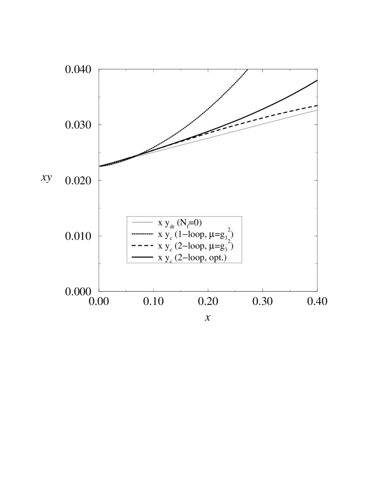
The use of 2-loop effective potential allows the construction of the critical curve $y_{c}(x)$ beyond 1-loop level. The numerical computation is shown in Fig. 1.

Refer to caption

Figure 1: The critical curve $y=y_{c}(x)$ (multiplied by $x$) computed from 1- and 2-loop potentials in the SU(2)+adjoint Higgs theory. Two of the curves are plotted for the scale choice $\mu=g_{3}^{2}$; $\mu$ for the second 2-loop curve is determined by optimization [8]. The scale dependence should give an estimate of higher order corrections. The thin curve is $y_{4d\to 3d}(x)$ from eq. (2.29). For $x\to 0$ all curves approach $2/(9\pi^{2})=0.0225$. The non-perturbative critical curve computed numerically is given in Fig. 3.

4 Z($N$) symmetry in the 3d theory

For $N_{f}=0$, hot SU($N$) gauge theory exhibits a Z($N$) symmetry [33, 31] so that there are $N$ equivalent ground states. In one of them $A_{0}=0$, in the others $A_{0}^{N^{2}-1}\sim 2\pi T/g$. In the weak coupling limit the field in the other minima thus becomes large. One can associate the QCD phase transition with the breaking of this symmetry so that at high temperatures one sits in one of the equivalent minima, say $A_{0}=0$. As one goes to lower temperatures, the barrier between the minima is becoming lower and at $T_{c}$, the symmetry is supposed to get restored. If one wants to apply a 3d theory down to temperatures close to $T_{c}$, it is thus important to discuss the role of the Z($N$) symmetry in 3d.

The construction of the super-renormalizable effective 3d field theory in Sec. 2 requires small amplitudes of the adjoint field $A_{0}$, $A_{0}\ll 2\pi T/g$. In practice, this means that one works around the $A_{0}=0$ minimum in the reduction step, so that the effective theory describes reliably only fluctuations of magnitude $\delta A\mathop{\raise 1.29167pt\hbox{$<$\kern-7.5pt\raise-4.73611pt\hbox{$\sim$}}}\pi T$ around that minimum. Thus, the price one pays for the simple effective theory is that the Z($N$) symmetry is not reproduced by it.

Some remnant of the Z($N$) symmetry nonetheless remains in the 3d theory. The effective theory will on its critical curve still contain $N$ metastable states but these are not completely equivalent, e.g., the correlators measured in them are different. As discussed, only the correlators in the symmetric phase ($A_{0}=0$) reliably represent 4d physics.

Indeed, within the interval $0<A_{0}^{3}<2\pi T/g$, eq. (3.6) at $y_{c}$ is seen to be the same as the 4d 1-loop potential in an $A_{0}^{3}$ background:

$\displaystyle V(A_{0}^{3})$ $\displaystyle=$ $\displaystyle{2\pi^{2}\over 3}T^{4}\biggl{[}B_{4}(0)+2B_{4}\biggl{(}{gA_{0}^{3}\over 2\pi T}\biggr{)}\biggr{]}$
$\displaystyle=$ $\displaystyle-{6\pi^{2}\over 90}T^{4}+{\frac{1}{3}}g^{2}T^{2}(A_{0}^{3})^{2}+{1\over 12\pi^{2}}g^{4}(A_{0}^{3})^{4}-{1\over 3\pi}g^{3}T(A_{0}^{3})^{3},\quad 0<A_{0}^{3}<{2\pi T\over g},$

where

$$B_{4}(x)\equiv-{1\over 30}+(x\,{\rm mod}1)^{2}[1-(x\,{\rm mod}1)]^{2}.$$ (4.2)

The effective potential (4) exhibits the Z(2) symmetry of the full 4d theory as the periodicity in $A_{0}^{3}$ with period $2\pi T/g$; this symmetry is not explicit in the effective theory on the tree level, but it is partly reinstated by radiative effects as seen in eq. (3.6). This is not surprising: in deriving the 4d 1-loop potential one performs a frequency sum over $n=0,\pm 1,\pm 2,...$. In deriving the couplings of the 3d theory one performs basically a frequency sum over $n=\pm 1,\pm 2,...$, and the $n=0$ mode enters when computing the effective potential within the 3d theory. Note also that (3.7) is exactly the same as the leading term in (2.29).

Thus, while the Z(2) symmetry is not explicit in the effective action, the second degenerate minimum is generated radiatively. Even with all higher order corrections in the non-perturbative solution of the 3d theory there will be two (for $N=2$) degenerate minima at some values of the 3d parameters, but this will no longer take place at any temperature $T>T_{c}$. Moreover, while these states are completely equivalent in the original 4d theory, the correlators measured in them will be different in the effective theory, the symmetric phase being the physical one. For SU(3) the full 4d theory has 3 equivalent states while in the 3d theory presumably only two of them have the same correlators; these are the unphysical ones corresponding to a large value $\sim 2\pi T/g$ of the fields.

5 Lattice analysis

5.1 Discretization

The lattice action corresponding to the continuum theory (2.6) is $S=S_{W}+S_{A}$ where

$$S_{W}=\beta_{G}\sum_{x}\sum_{i<j}(1-{\frac{1}{2}}{\rm Tr\,}P_{ij})$$ (5.1)

is the standard SU(2) Wilson action and, in continuum normalization ($A_{0}=A_{0}^{a}T_{a}$) and for $\bar{\lambda}_{A}=0$,

$\displaystyle S_{A}$ $\displaystyle=$ βˆ‘x,i2​[Tr​a​A02​(x)βˆ’Tr​a​A0​(x)​Ui​(x)​A0​(x+i)​Ui†​(x)]subscriptπ‘₯𝑖2delimited-[]Trπ‘Žsuperscriptsubscript𝐴02π‘₯Trπ‘Žsubscript𝐴0π‘₯subscriptπ‘ˆπ‘–π‘₯subscript𝐴0π‘₯𝑖superscriptsubscriptπ‘ˆπ‘–β€ π‘₯\displaystyle\sum_{x,i}2\biggl{[}{\rm Tr\,}aA_{0}^{2}(x)-{\rm Tr\,}aA_{0}(x)U_{i}(x)A_{0}(x+i)U_{i}^{\dagger}(x)\biggr{]} (5.2)
$\displaystyle+\sum_{x}\biggl{[}(m_{D}a)^{2}{\rm Tr\,}aA_{0}^{2}(x)+a\lambda_{A}({\rm Tr\,}aA_{0}^{2})^{2}\biggr{]},$

where

$$a={4\over\beta_{G}g_{3}^{2}}$$ (5.3)

is the lattice spacing and $m_{D}$ is the bare mass in the lattice scheme. Renormalisation is carried out so that the physical results are the same as in the $\overline{\mbox{\rm MS}}$ scheme with the renormalized mass parameter

$$m_{D}^{2}(\mu)=\biggl{(}y+{20x-10x^{2}\over 16\pi^{2}}\ln{g_{3}^{2}\over\mu}\biggr{)}g_{3}^{4}.$$ (5.4)

The resulting counterterms have been computed in [24] with the result

$$m_{D}^{2}=m_{D}^{2}(\mu)-{\Sigma\over 4\pi a}(4g_{3}^{2}+5\lambda_{A})-{g_{3}^{4}\over 16\pi^{2}}\biggl{[}(20x-10x^{2})(\ln{6\over a\mu}+0.09)+8.7+11.6x\biggr{]},$$ (5.5)

where $\Sigma=3.1759114$. There are no higher order corrections to this relation in the limit $a\to 0$. For 1-loop $O(a)$-improvement, see [25].

The action can be written in different forms by rescalings of $A_{0}$. For example, replacing $A_{0}$ by an anti-Hermitian matrix [21, 22] by $aA_{0}^{2}\equiv-\beta_{A}\tilde{A}_{0}^{2}/4$, gives an action of the form

SA=Ξ²Aβ€‹βˆ‘x,i12​Tr​A~0​(x)​Ui​(x)​A~0​(x+i)​Ui†​(x)+βˆ‘x[βˆ’Ξ²2​12​Tr​A~02+Ξ²4​(12​Tr​A~02)2],subscript𝑆𝐴subscript𝛽𝐴subscriptπ‘₯𝑖12Trsubscript~𝐴0π‘₯subscriptπ‘ˆπ‘–π‘₯subscript~𝐴0π‘₯𝑖superscriptsubscriptπ‘ˆπ‘–β€ π‘₯subscriptπ‘₯delimited-[]subscript𝛽212Trsuperscriptsubscript~𝐴02subscript𝛽4superscript12Trsuperscriptsubscript~𝐴022S_{A}=\beta_{A}\sum_{x,i}{\frac{1}{2}}{\rm Tr\,}\tilde{A}_{0}(x)U_{i}(x)\tilde{A}_{0}(x+i)U_{i}^{\dagger}(x)+\sum_{x}\biggl{[}-\beta_{2}{\frac{1}{2}}{\rm Tr\,}\tilde{A}_{0}^{2}+\beta_{4}({\frac{1}{2}}{\rm Tr\,}\tilde{A}_{0}^{2})^{2}\biggr{]}, (5.6)

where

$${\beta_{2}\over\beta_{A}}=3+{8y\over\beta_{G}^{2}}-{\Sigma(4+5x)\over 2\pi\beta_{G}}-{1\over 2\pi^{2}\beta_{G}^{2}}\biggl{[}(20x-10x^{2})(\ln{{\frac{3}{2}}\beta_{G}}+0.09)+8.7+11.6x\biggr{]}$$ (5.7)

and

$$\beta_{4}={x\over\beta_{G}}\beta_{A}^{2}.$$ (5.8)

Since there are two dimensionless parameters, one more arbitrary choice is possible. In fundamental Higgs theories one often scales the coefficient of the quadratic term to unity; here we choose $\beta_{A}=\beta_{G}$.

As the final relation, one wants to determine the continuum theory value of $\langle A_{0}^{a}A_{0}^{a}\rangle$ when doing simulations with the lattice action (5.1)+(5.6) with $\beta_{A}=\beta_{G}$. The answer is

$${\langle A_{0}^{a}A_{0}^{a}\rangle\over 2g_{3}^{2}}={\beta_{G}^{2}\over 8}\biggl{[}-\langle{\frac{1}{2}}{\rm Tr\,}\tilde{A}_{0}^{2}\rangle-{3\Sigma\over 4\pi\beta_{G}}-{3\over\beta_{G}^{2}\pi^{2}}\biggl{(}\log{3\beta_{G}\over 2}+0.67\biggr{)}\biggr{]}.$$ (5.9)

5.2 Simulations

The aim of the simulations is as follows:

  • β€’

    Find the critical curve $y=y_{c}(x)$ and, in particular, its endpoint $x_{\rm end}$. This is done by measuring the distributions of ${\rm Tr\,}A_{0}^{2}$ (or some other operator) at fixed $x$, finding a two-state signal and the $V\to\infty,a\to 0$ limit of the value of $y$ at which this happens,

  • β€’

    Measure the correlator masses on both sides of the transition line and in the cross-over region $x>x_{\rm end}$.

It is important to estimate the required lattice volume $V$ and constant $a$ (or $\beta_{G}$). In the broken phase, on the tree level we have at least two relevant mass scales, the adjoint scalar mass $\approx gT$ from eq. (3.2) and the vector mass $g\langle A_{0}^{3}\rangle=2\pi T$ from eq. (3.3). Thus, in order to describe accurately the broken phase, we must demand

$$a\ll{1\over 2\pi T}\ll{1\over gT}\ll Na.$$ (5.10)

These convert to

$$\beta_{G}\gg{8\over 3\pi x},\qquad N\gg{\pi\sqrt{3}\over 4}\beta_{G}\sqrt{x}.$$ (5.11)

For the symmetric phase the scale $2\pi T$ is absent, so that the requirement on $\beta_{G}$ is not quite as demanding, $\beta_{G}\gg 1$.

The simulations were performed with a Cray C90 at the Finnish Center for Scientific Computing, and the total cpu-time usage was 760 cpu-hours.

5.3 The phase diagram
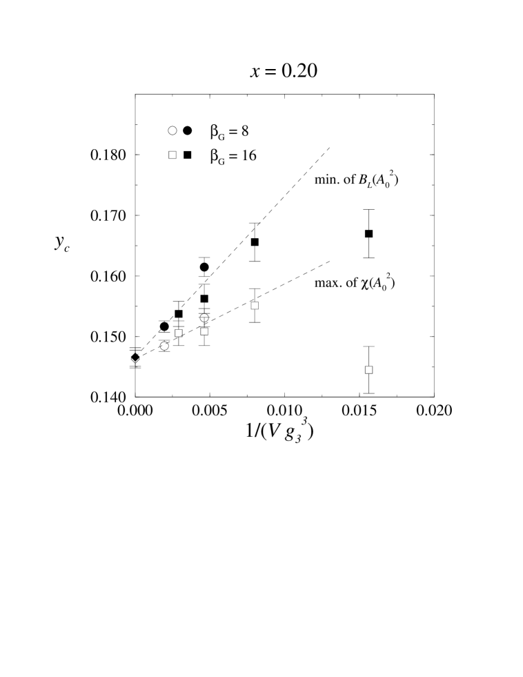
We locate the transition line $y=y_{c}(x)$ by using ${\rm Tr\,}A_{0}^{2}$ as an order parameter. For each lattice size, we define the pseudocritical  $y$ with the following commonly used methods [34]: (a) maximum of the susceptibility $\chi(A_{0}^{2})=\langle({\rm Tr\,}A_{0}^{2}-\langle{\rm Tr\,}A_{0}^{2}\rangle)^{2}\rangle$; (b) minimum of the 4th order Binder cumulant $B_{L}(A_{0}^{2})=1-\langle({\rm Tr\,}A_{0}^{2})^{4}\rangle/(3\langle({\rm Tr\,}A_{0}^{2})^{2}\rangle^{2})$; and, when the transition is strongly 1st order, (c) the β€œequal weight” criterion for the probability distribution $p({\rm Tr\,}A_{0}^{2})$. For any finite volume, these criteria give different pseudocritical values of $y$, but they all extrapolate to the same limit when $V\rightarrow\infty$. This extrapolation is shown in Fig. 2 for $x=0.20$.

Refer to caption

Figure 2: The $y_{c}$ extrapolation to $V\rightarrow\infty$ for $x=0.20$. Within the statistical errors, there is no lattice spacing $\beta_{G}$ dependence.

The analysis is repeated for several $\beta_{G}$, corresponding to different lattice spacings through eq. (5.3). In our case, as long as the conditions (5.11) are satisfied, we found no appreciable lattice spacing dependence in the results. This is also evident in Fig.2.

Our result for the phase diagram of the continuum SU(2)+adjoint Higgs model is shown in Fig. 3. As already pointed out in [29], the phase diagram consists of a first-order line which terminates, so that the two β€œphases” are analytically connected. We find the endpoint to be close to $x_{\rm end}=0.3$. As can be seen from the figure, the results are independent of $\beta_{G}$ well within the statistical accuracy. However, the infinite volume extrapolation is essential, as shown by some large but finite volume points in Fig. 3.
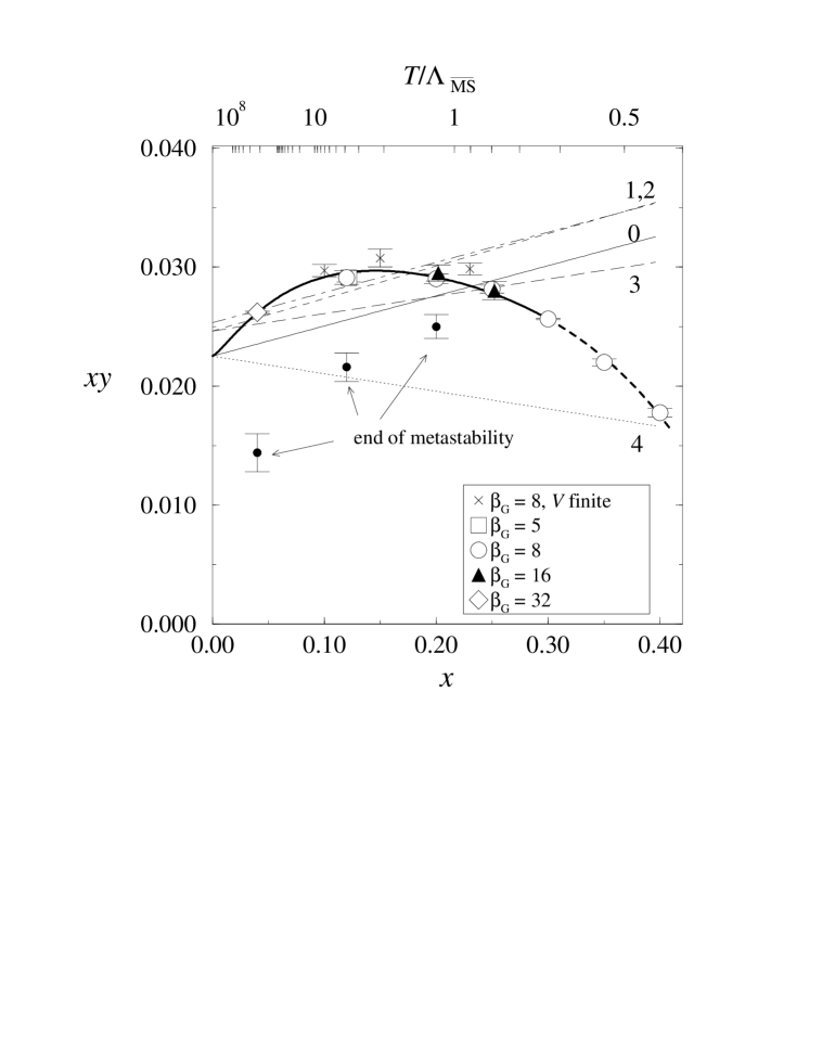
Refer to caption

Figure 3: Data points in the limit $V\to\infty,a\to 0$ for the critical curve $y=y_{c}(x)$ (multiplied by $x$). The thick line is the 4th order fit (5.12) to the $V=\infty$ extrapolated data. The dashed line marks the region where the transition turns into a cross-over. The straight lines are the 4d$\to$3d curves of eq. (2.27) marked by the value of $N_{f}$. The top scale shows the values of $T/\Lambda_{\overline{\rm MS}}$ corresponding to the values of $x$ for $N=2,N_{f}=0$, obtained using eq. (2.26). The physical implications of the figure are discussed in Sec. 6.

The thick transition line $y_{c}(x)$ in Fig. 3 has been obtained with a fit to the $V\rightarrow\infty$ -extrapolated results, as

$$xy_{c}=2/(9\pi^{2})(1+9/8x+Ax^{3/2}+Bx^{2}+Cx^{5/2}+Dx^{3}),$$ (5.12)

where $A=45.1(2.9),~{}B=-214.7(20.2),~{}C=350.7(44.5),~{}D=-206.7(31.4)$. The fit has been constrained to join the curve $xy_{4d\to 3d}(x)$ and its slope when $x\rightarrow 0$. We used fractional powers of $x$ in the fit since in the perturbative expansion of the critical curve terms like $g_{3}^{2}/m_{D}\sim{\sqrt{x}}$ appear. There can also be logarithms in the expansion.

It is interesting that the behaviour of the 3d SU(2) + adjoint Higgs model is quite different from that of the 3d SU(2) + fundamental Higgs theory studied earlier [12]. First, in the fundamental case the value of $y_{c}$ was smaller than the 2-loop perturbative result for all values of $x$, while in the adjoint case the situation is opposite for $x<0.2$ (compare Figs. 1, 3). Second, the magnitude of the higher order perturbative or non-perturbative effects is much larger in the adjoint case. To get a feeling of the difference, suppose that the deviation from the perturbative result comes entirely from a non-perturbative energy shift at $A_{0}=0$ [35, 12],

$$\delta V=\frac{1}{12}A_{F}g_{3}^{6},$$ (5.13)

where $A_{F}$ is some constant to be determined numerically. For the fundamental case this was estimated to be $A_{F}\simeq-0.08$ at $x\sim 0.06$. A first order estimate of the change in the critical value,

$${\frac{1}{2}}\delta m_{D}^{2}A_{0}^{2}=-\delta V,$$ (5.14)

gives in the present case

$$A_{F}\simeq-\frac{8}{3\pi^{2}}\frac{\delta y_{c}}{x^{2}}.$$ (5.15)

For example, for $x=0.04$ we have $A_{F}\sim 10$ ($\sim 100$ times larger than in the fundamental case!) and for $x=0.12$, $A_{F}\sim 0.4$. We do not have any clear understanding of this huge difference. From the point of view of perturbation theory, both cases are quite similar. The only difference we see is that the adjoint theory contains instantons (monopoles) in the broken phase, while the fundamental does not.

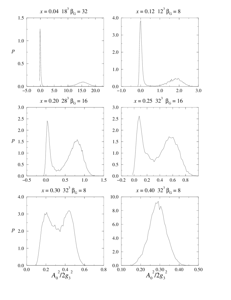
In Fig. 4 we show the probability distributions $p(A_{0}^{2})$, measured with various values of $x$ along the transition line $y_{c}(x)$. When $x\sim 0.04$, the transition is extremely strongly first order, as evidenced by the strong separation of the two peaks in the distribution. Indeed, for $x\leq 0.12$ we use the multicanonical algorithm in order to enhance the tunnelling from one phase to another – this is absolutely necessary in order to ensure the correct statistical weights for the phases. When $x$ increases, the transition becomes weaker, and at $x=0.40$ we see no sign of a transition any more.

Due to the strong 1st order transition, there is a substantial metastability  range in $y$ around the transition line at small $x$. Within this range the thermodynamically unstable state can be stable enough so that, for practical purposes ($\sim$ measurements), it behaves as if it were stable. In Fig. 3 we show the lower end of the symmetric phase metastability range for $x=0.04$, 0.12 and 0.20. This has been obtained by reweighting the $y_{c}(x)$ -distributions (Fig. 4) to smaller values of $y$ until the peak of the distribution corresponding to the symmetric phase vanishes.

Refer to caption

Figure 4: The probability distributions of $A_{0}^{a}A_{0}^{a}/2g_{3}^{2}={\frac{1}{N_{S}^{3}}}\sum_{x}A_{0}^{a}A_{0}^{a}/2g_{3}^{2}$, measured at various locations on the transition line $y=y_{c}(x)$.

The behaviour of $\langle A_{0}^{a}A_{0}^{a}\rangle/2g_{3}^{2}$ when crossing the transition line or its continuation is shown in Fig. 5.

Refer to caption

Refer to caption

Figure 5: The behaviour of $\langle A_{0}^{a}A_{0}^{a}\rangle/2g_{3}^{2}$ in continuum normalization (see eq. (5.9)) when crossing the phase transition at $x=0.12$ and the cross-over at $x=0.35$.

5.4 Correlator masses

The list of gauge-invariant composite operators of lowest dimensionality is:

  • β€’

    Dim = 1: the scalar ${\rm Tr\,}A_{0}^{2}$,

  • β€’

    Dim = 3/2: the vector $h_{i}=\epsilon_{ijk}A_{0}^{a}F_{jk}^{a}$,

  • β€’

    Dim = 2: the scalar $({\rm Tr\,}A_{0}^{2})^{2}$,

  • β€’

    Dim = 3: the scalars $({\rm Tr\,}A_{0}^{2})^{3}$ and $G=F_{ij}^{a}F_{ij}^{a}$ and the tensor $F_{ij}^{a}F_{jk}^{a}$.

Perturbatively the Lagrangian (2.6) for $N=2$ in the symmetric phase has 3$\times$2 massless vector ($A_{i}^{a}$) and 3 scalar ($A_{0}^{a}$) degrees of freedom. Because of confinement, only SU(2) singlets appear in the spectrum. Thus, the above mentioned operators represent bound states in the symmetric phase. For example, ${\rm Tr\,}A_{0}^{2}$ is a bound state of two adjoint scalar β€œquarks”, $h_{i}$ is a bound state of an adjoint quark and light glue, and $G$ is a scalar glueball state.

In the limit of large $y\gg 1$ the SU(2) theory under consideration in the symmetric phase can be considered an analog of QCD with heavy scalar adjoint quarks. Thus, a number of statements can be made on the expected spectrum with the use of the heavy quark expansion. First, the lowest energy states are different types of glueballs with $m_{G}\sim g_{3}^{2}$. Next, we have a bound state $h_{i}$ of the scalar quark and gluon with the mass $m_{h}=m_{D}+O(g_{3}^{2})$, $m_{D}=\sqrt{y}g_{3}^{2}$. The leading correction to $m_{h}$ can be determined:

$$m_{h}-m_{D}=\frac{g_{3}^{2}}{2\pi}\log\sqrt{y}+\frac{c}{2\pi}g_{3}^{2}+...$$ (5.16)

The coefficient in front of the log is a result of a perturbative computation of the pole $A_{0}$ mass in [36], whereas the constant term proportional to $g_{3}^{2}$ cannot be computed perturbatively. In fact, the mass of this bound state coincides with the non-perturbative definition of the Debye screening mass, discussed in [37]. Finally, the mass of the bound state $A_{0}^{2}$ is expected to be

$$m(A_{0}^{2})=2\sqrt{y}g_{3}^{2}+O(g_{3}^{2}).$$ (5.17)

In the broken phase the perturbative spectrum consists of 2$\times$3 massive vectors ($W^{\pm}$), $m_{W}\simeq 2g_{3}^{2}/(3\pi x)$, 2 massless vectors (the photon $\gamma$) and one scalar degree of freedom (the Higgs) with mass $\simeq m_{D}$. The 2$\times$3 massive vector states $W^{\pm}$ have U(1) charges and thus are not gauge invariant. Moreover, in 3d the U(1) Coulomb potential is logarithmically divergent, and thus the U(1) charged states (like $W$) must be absent from the spectrum. Therefore, the following set of gauge-invariant operators should describe the spectrum of the theory in the β€œbroken” phase: ${\rm Tr\,}A_{0}^{2}$ for the Higgs excitation, $h_{i}$ for the β€œphoton”, and $G$ for the bound state of the massive $W$’s. In fact, to obtain in the unitary gauge $\hat{A}_{0}^{a}\equiv A_{0}^{a}/\sqrt{A_{0}^{b}A_{0}^{b}}=\delta_{a3}$ a pure photon operator, one may take [26]

$$\gamma_{ij}=\hat{A}_{0}^{a}F_{ij}^{a}-{1\over g_{3}}\epsilon_{abc}\hat{A}_{0}^{a}(D_{i}\hat{A}_{0})^{b}(D_{j}\hat{A}_{0})^{c}.$$ (5.18)

However, in our measurements this operator was dominated by the first term, yielding similar results as the operator $h_{i}$. As discussed in the introduction, the broken phase tree-level massless photon is actually replaced by a massive pseudoscalar excitation.

In the following we constrain ourselves to the study of three different operators, ${\rm Tr\,}A_{0}^{2}$, $h_{i}$ and $G$. Our strategy is the following: first, we are going to consider correlation functions near the 3d transition line. This will allow us to compare masses of different excitations in the vicinity of the phase transition, as well as to determine correlation lengths in the symmetric phase (as we will discuss later, this is the physical phase from the 4d point of view) along the 4d $\rightarrow$ 3d dimensional reduction curve. Second, we make measurements at some fixed $x$ for different values of $y$ in the symmetric phase, in order to check different hypotheses concerning the spectrum of the bound states and in order to determine non-perturbatively the Debye screening mass and the $O(g^{2}T)$ correction to it.

The correlation functions are measured in the direction of the $x_{3}$ -axis, and to enhance the projection to the ground states, we use blocking  in the $(x_{1},x_{2})$-plane. The fields are recursively mapped from blocking level $(k)\rightarrow(k+1)$, so that the fields on the $(k+1)$-level lattice are defined only on even points of the $(k)$-level lattice on the $(x_{1},x_{2})$-planes:

A0(k+1)​(y)=15​A0(k)​(x)+15β€‹βˆ‘i=Β±1,2Ui(k)​(x)​A0(k)​(x+i)​Ui(k)⁣†​(x)superscriptsubscript𝐴0π‘˜1𝑦15superscriptsubscript𝐴0π‘˜π‘₯15subscript𝑖plus-or-minus12subscriptsuperscriptπ‘ˆπ‘˜π‘–π‘₯superscriptsubscript𝐴0π‘˜π‘₯𝑖subscriptsuperscriptπ‘ˆπ‘˜β€ π‘–π‘₯A_{0}^{(k+1)}(y)={\frac{1}{5}}A_{0}^{(k)}(x)+{\frac{1}{5}}\sum_{i=\pm 1,2}U^{(k)}_{i}(x)A_{0}^{(k)}(x+i)U^{(k)\dagger}_{i}(x) (5.19)

and (i=1,2,jβ‰ iformulae-sequence𝑖12𝑗𝑖i=1,2,j\neq i)

$\displaystyle U^{(k+1)}_{i}(y)$ $\displaystyle=$ $\displaystyle U^{\prime(k)}_{i}(x)U^{\prime(k)}_{i}(x+i),$ (5.20)
$\displaystyle U^{\prime(k)}_{i}(x)$ $\displaystyle=$ 13​Ui(k)​(x)+13β€‹βˆ‘j=Β±1,2Uj(k)​(x)​Ui(k)​(x+j)​Uj(k)⁣†​(x+i).13subscriptsuperscriptπ‘ˆπ‘˜π‘–π‘₯13subscript𝑗plus-or-minus12subscriptsuperscriptπ‘ˆπ‘˜π‘—π‘₯subscriptsuperscriptπ‘ˆπ‘˜π‘–π‘₯𝑗subscriptsuperscriptπ‘ˆπ‘˜β€ π‘—π‘₯𝑖\displaystyle{\frac{1}{3}}U^{(k)}_{i}(x)+{\frac{1}{3}}\sum_{j=\pm 1,2}U^{(k)}_{j}(x)U^{(k)}_{i}(x+j)U^{(k)\dagger}_{j}(x+i). (5.21)

The scalar and vector operators above are then calculated from the blocked fields. The blocking is repeated up to 4 times, and the correlation functions are measured for each blocking level separately. For each operator and coupling constant we select the blocking level which yields the best exponential fits; typically level 3 or 4.

Because we expect the vector operator $h_{i}$ to yield a very light mass value in the broken phase, we measure it in the lowest non-zero transverse momentum channel (for all of the blocking levels), in addition to the zero momentum channel:

$$O_{3}(x_{3})={\frac{1}{N_{S}^{2}}}\sum_{x_{1},x_{2}}A_{0}^{a}F_{12}^{a}e^{i2\pi x_{1}/N_{S}}.$$ (5.22)

The screening mass is then extracted from the asymptotic behaviour of $\langle O_{3}(0)O_{3}(x_{3})\rangle\!\propto\exp[-Wx_{3}]$, where

$$W=\sqrt{(2\pi/N_{S})^{2}+m_{\gamma}^{2}}.$$ (5.23)

Refer to caption

Refer to caption

Figure 6: The correlator masses of the operators ${\rm Tr\,}A_{0}^{2}$ and $h_{i}=\epsilon_{ijk}{\rm Tr\,}A_{0}F_{jk}$ measured when crossing the phase transition at $x=0.12$ and the cross-over at $x=0.35$.

The results for the masses both in the 1st order phase transition region ($x=0.12$) and the cross-over region ($x=0.35$) are shown in Fig. 6. At the phase transition the masses exhibit a prominent discontinuity. In the broken phase $y<y_{c}$ there is a photon of very small mass and a scalar the mass of which is close to the mass parameter $m_{D}$; in these units $\sqrt{2/3}gT/g^{2}T=\sqrt{2/(9\pi^{2}x)}$. In the broken phase only the non-zero transverse momentum operator gives statistically significant results for $h_{i}$. The negative mass values in Fig. 6 notify negative $m_{\gamma}^{2}$-values, as obtained from the relation (5.23). The photon mass is statistically consistent with zero but, as discussed already in [29], a small non-zero photon mass is not excluded. This is required for the analytic connection between the two β€œphases”; otherwise the photon mass could act as an order parameter separating the phases (this, in fact, is what happens in the U(1)+Higgs case, the Ginzburg-Landau theory [38]). In the symmetric phase $y>y_{c}$ there is a scalar $A_{0}-A_{0}$ and a vector $A_{i}-A_{0}$ bound state of rather large mass. In the cross-over region the mass of the scalar state dips at $y=y_{c}$ while that of the vector state increases monotonically.
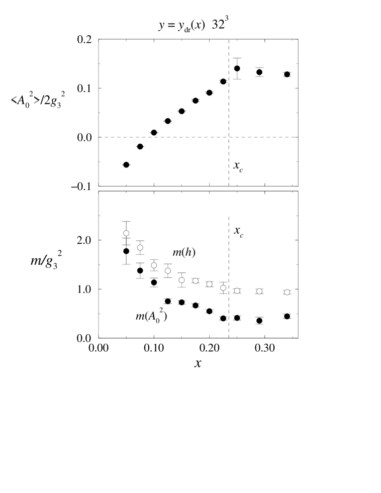
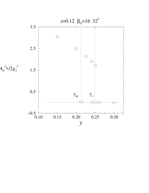
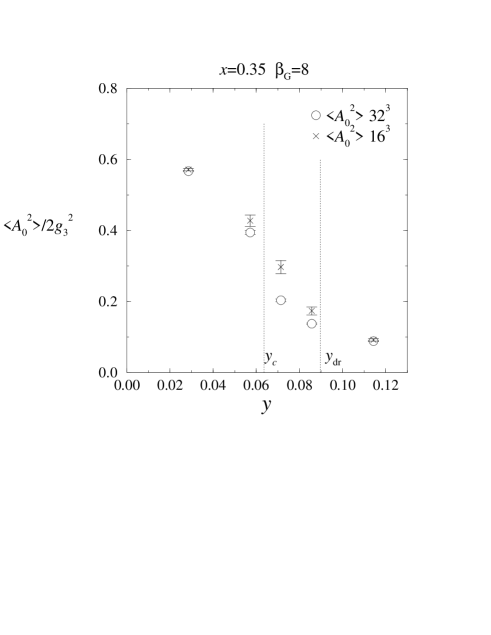
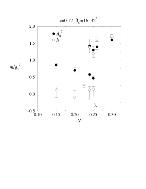
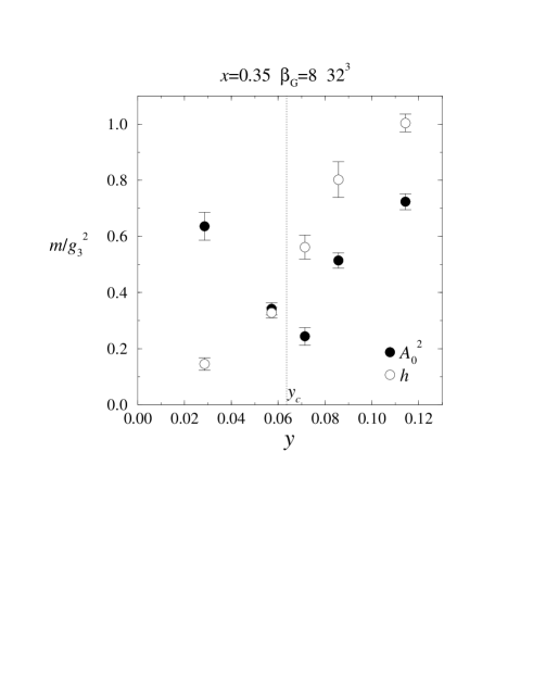
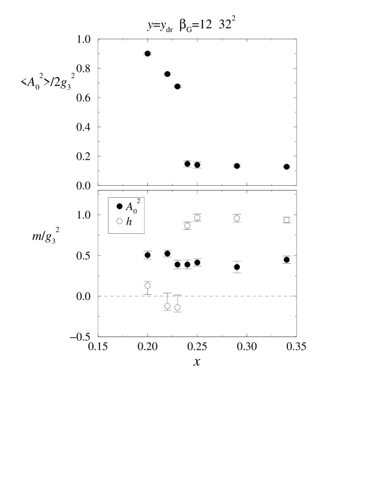
Refer to caption

Figure 7: The order parameter $\langle A_{0}^{a}A_{0}^{a}\rangle/2g_{3}^{2}$ and the scalar and vector masses $m(A_{0}^{2})$, $m(h)$ in the symmetric phase along $y=y_{4d\to 3d}(x)$. When $x<x_{c}\approx 0.235$, the symmetric phase is metastable. The $x<x_{c}$ -points have been calculated with $\beta_{G}=8$, $x>x_{c}$ with $\beta_{G}=12$.

Now, consider the masses of $A_{0}^{2}$ and $h_{i}$ in the symmetric phase along the dimensional reduction curve $y=y_{4d\to 3d}(x)$, Fig. 7. These measurements are possible since for $x<0.235$ the symmetric phase is metastable with a sufficiently long tunneling time, while at $x>0.235$ it is absolutely stable. As one can see the expectation $m(A_{0}^{2})/m(h)\simeq 2$ is strongly violated in the whole region of $x$ studied, $x>0.05$. This indicates that the corrections to the leading order results (5.16), (5.17) are large. In order to clarify this point, we study different correlators at large values of $y$ and and fixed x, where the heavy quark expansion is expected to be valid.

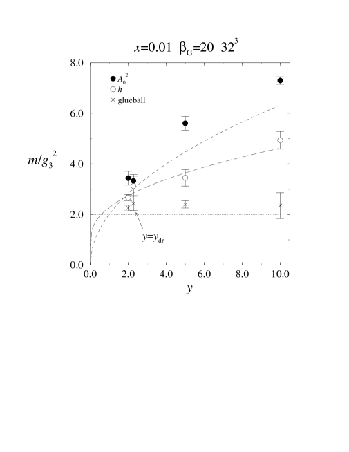
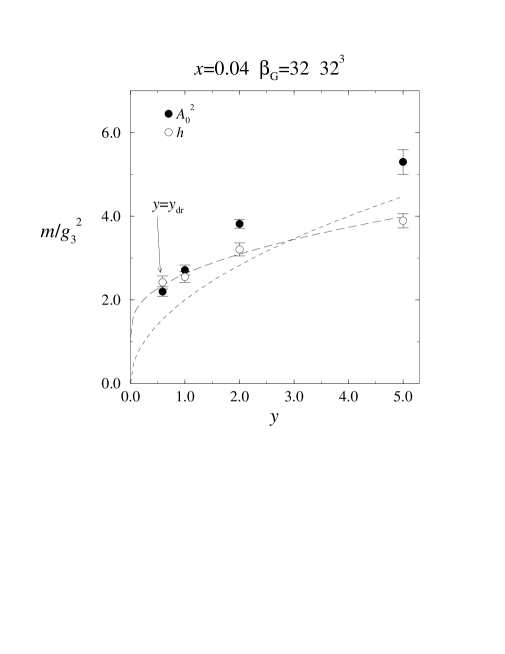
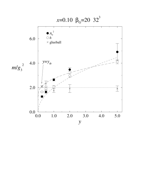
In Fig. 8 we show the dependence of the masses of the bound states on $y$ at different values of $x$, $x=0.01,0.04,0.10$. As expected, the glueball mass does practically not depend on $y$ or $x$, while the $A_{0}^{2}$ and $h_{i}$ masses have some dependence on $x$. Moreover, at large $y$, $m(A_{0}^{2})>m(h)$ as it should be. A fit to the data allows to fix the unknown coefficient $c$ in (5.16). Only sufficiently large values of $y$ should be used, $\sqrt{y}>c$, to make sure that the correction is smaller than the leading contribution. We found for $y>2$:

$\displaystyle x$ $\displaystyle=$ $\displaystyle 0.10:c=1.74(16)\cdot(2\pi),$
$\displaystyle x$ $\displaystyle=$ $\displaystyle 0.04:c=1.53(17)\cdot(2\pi),$
$\displaystyle x$ $\displaystyle=$ $\displaystyle 0.01:c=1.39(20)\cdot(2\pi).$ (5.24)

This indicates a slight $x$-dependence of the parameter $c$, which is perhaps a result of higher order corrections. A linear in $x$ fit works very well, and the intercept represents a realistic estimate for c,

$$c=1.36(18)\cdot(2\pi).$$ (5.25)

This is basically the same as the result of the x=0.01 point.

The large value of the coefficient $c$ explains why the heavy quark expansion does not work for the values of $x$ considered in Fig. 7 along the dimensional reduction curve $y=y_{4d\to 3d}(x)$. The adjoint β€œquark” can be considered heavy only if $\sqrt{y}>{c}/(2\pi)$, which gives $x<{8}/(9c^{2})\simeq 0.01$.

Refer to caption

Refer to caption

Refer to caption

Figure 8: Scalar, vector and glueball bound state masses for $x=0.01,~{}0.04,~{}0.10$.

6 The physical phase of the 3d theory

The previous simulation results were entirely for the 3d effective SU(2)+adjoint Higgs theory as such. We can now return to the main question: what is their relevance for the 4d finite temperature $N=2$ QCD?

According to the 2-loop dimensional reduction in Sec. 2, the physical 4d theories, defined by the values of $T/\Lambda_{\overline{\rm MS}},N=2,N_{f}$, lie on the straight lines $y_{4d\to 3d}(x)$ (eq.(2.27)) plotted in Fig. 3. Consider first the quarkless case, $N_{f}=0$. One observes that for almost all the range $x<x_{\rm end}\sim 0.30$, one has $y_{4d\to 3d}(x)<y_{c}(x)$ as already suggested by the 2-loop computations in Fig. 1. Thus superficially, the finite temperature 4d theory corresponds to the broken phase of the 3d theory. This was the conclusion reached in [39] (the status of which is reviewed in [40]).

However, this conclusion cannot be right. The 3d broken phase is a remnant of the 4d Z(2)-symmetry as discussed in Sec. 4, and the derivation of the effective theory is not reliable there. Instead, the physical phase must be the (in the 4d language, equivalent) symmetric phase where the 3d theory can be trusted. Indeed, at $y=y_{4d\to 3d}(x)$ the symmetric phase of the 3d theory is metastable in the whole region of $x$, and all the observables can be measured within the metastable phase, see Fig. 7. That the symmetric phase is the physical phase of the 3d theory was the conclusion reached in [22], as well; however, there the 3d symmetric phase was seen to be stable. The difference is due to increased accuracy in relating continuum and lattice results. If one would be able to construct a 3d theory which fully respects the Z($N$) symmetry, then the metastable phase should be promoted to a stable phase in coexistence with its Z(2) companion.

Refer to caption

Figure 9: The order parameter $\langle A_{0}^{a}A_{0}^{a}\rangle/2g_{3}^{2}$ and the scalar and vector masses $m(A_{0}^{2})$, $m(h)$ in the stable phase along $y=y_{4d\to 3d}(x)$. For $x<0.235$ the stable phase is the broken phase, for $x>0.235$ the symmetric phase (see Fig. 3). As discussed in Sec. 6, at $x<0.235$ it is rather the metastable symmetric phase which is physical.

What happens when one goes to smaller $T$ (larger $x$), towards $T_{c}$? Then the 3d theory is becoming less reliable even in the symmetric phase, for several reasons. First, the perturbative expansion for the parameters of the 3d theory is becoming less reliable, see eq. (2.29). Moreover, the higher order operators are becoming more important since the mass hierarchy between the scales $g_{3}^{2},\pi T$ is lost due to increasing $g^{2}(T)$ at $T/\Lambda_{\overline{\rm MS}}<{\rm\mbox{a few}}$, see Sec. 2. Indeed, the masses of the excitations in the 3d theory are $\sim g_{3}^{2}$, see Fig. 7, so they need then no longer be the dominant infrared excitations.

In Fig. 9, the order parameter and the masses have been plotted in the stable phase corresponding to $y=y_{4d\to 3d}(x)$. One sees that at $x\sim 0.235$ the symmetric phase becomes stable. But this corresponds to $T/\Lambda_{\overline{\rm MS}}\approx 0.9$, where the 3d theory is no longer reliable and the QCD phase transition has already taken place. Thus this β€œtransition” is not related to the 4d QCD transition.

Consider then the endpoint value, $x_{\rm end}\sim 0.30$ (see Fig. 3). This corresponds to $T/\Lambda_{\overline{\rm MS}}\approx 0.6$ and is again below the value $T_{c}/\Lambda_{\overline{\rm MS}}=1.23(11)$ determined [32] for the SU(2) phase transition with 4d simulations. Yet the difference is not that large, and it is tempting to conjecture that if one had a 3d theory fully respecting the Z($N$) symmetry, then the corresponding endpoint might represent the QCD phase transition.

Consider finally the $N_{f}$ dependence. Fermions do not appear as dynamical fields in the effective theory, and their only effect is through the parametric dependence on $N_{f}$. At very small $x$ (very large $T$) the curves in Fig. 3 imply that the system lies in the symmetric phase near $A_{0}=0$. This result is in agreement with the fact that quarks break the Z(2) symmetry: the second minimum becomes metastable for $N_{f}=1$ and disappears for $N_{f}\geq 3$. At very large $N_{f}$, on the other hand, the perturbative expansion for the curves $y=y_{4d\to 3d}(x)$ gets worse.

7 Discussion

Dimensional reduction allows to construct an effective field theory for high temperature QCD, which is reliable as long as $g_{3}^{2}\ll\pi T$, implying $T\mathop{\raise 1.29167pt\hbox{$>$\kern-7.5pt\raise-4.73611pt\hbox{$\sim$}}}{\rm\mbox{a few}}\times T_{c}$. However, the effective super-renormalizable 3d gauge+adjoint Higgs theory does not describe the confinement-deconfinement phase transition.

The usual β€œpower counting” picture of correlation lengths in high temperature QCD says that the longest scale is related to the magnetic sector of the theory and is of order $(g^{2}T)^{-1}$. The shorter scale, $\sim(gT)^{-1}$, is associated with Debye screening. Our study shows that this picture is correct only at extremely high temperatures. First, the purely magnetic scale comes from the lowest glueball mass in a pure SU(2) theory, $m_{G}\sim 2g_{3}^{2}$. This should be compared with the leading order Debye mass $m_{D}^{2}\sim{\frac{2}{3}}g^{2}T^{2}$. The requirement $m_{D}>m_{G}$ tells that only at $x<0.005$ are the β€œmagnetic” effects numerically smaller than the β€œelectric” ones. A similar estimate follows from the requirement that the non-perturbative corrections to the Debye screening mass are on the level of, say, $50$ % of the tree-level value. In terms of temperature, this gives ridiculously large numbers. For example, for pure SU(2) this means $T>10^{35}\Lambda_{\overline{\rm MS}}$.

Thus, in the physically most interesting region somewhere above the critical temperature, the β€œnaive” picture is wrong. The longest correlation length corresponds to the $0^{++}$ bound state $A_{0}-A_{0}$ (in 3d language). In terms of 4d variables, this correlation length can be found from the analysis of Polyakov lines,

$$\langle L({\bf x})L^{\dagger}(0)\rangle\sim\exp[-m(A_{0}^{2})|{\bf x}|]/|{\bf x}|,$$ (7.1)

where

$$L({\bf x})={\rm Tr\,}\Omega({\bf x}),\quad\Omega({\bf x})={\cal P}\exp[ig\int_{0}^{\beta}\!d\tau\,A_{0}(\tau,{\bf x})].$$ (7.2)

The second largest correlation length is associated with Debye screening. In 3d language, it is related to the operator $h_{i}$. The corresponding 4d operators may be found in [37]. The non-perturbative Debye screening mass is about a factor $3$ larger than the lowest order estimate up to temperatures $T\sim 200\Lambda_{\overline{\rm MS}}$. The fact that the Debye mass is non-perturbative does not allow a reliable integration out of the $A_{0}$ field for the construction of the simplest effective field theory, containing only the scale $g_{3}^{2}$, unless the temperature of the system is extremely large.

Finally, the pure static glue sector has an even larger mass scale. In pure SU(2) and SU(2)$+$fundamental Higgs theories, $m_{G}\simeq 1.6g_{3}^{2}$ [15]; in the present theory we have measured $m_{G}$ to be almost the same.

It remains to be seen whether this modification of the standard picture of the high-temperature gauge theories has applications in the cosmological discussion of the quark-hadron phase transition or in heavy ion collisions.

Acknowledgements

We thank CSC-Tieteellinen laskenta Oy β€” the Finnish Center for Scientific Computing β€” for computational facilities, and C. Korthals Altes for useful discussions.

Appendix Appendix A

Some useful group theoretical relations for the SU(N) generators $T^{a}_{ij}$ in the fundamental representation are:

$\displaystyle T_{a}T_{b}$ $\displaystyle=$ 12​N​δa​b+12​da​b​s​Ts+i2​fa​b​s​Ts,12𝑁subscriptπ›Ώπ‘Žπ‘12subscriptπ‘‘π‘Žπ‘π‘ subscript𝑇𝑠𝑖2subscriptπ‘“π‘Žπ‘π‘ subscript𝑇𝑠\displaystyle{\frac{1}{2N}}\delta_{ab}+{\frac{1}{2}}d_{abs}T_{s}+{\frac{i}{2}}f_{abs}T_{s},
$\displaystyle T^{a}_{ij}T^{a}_{kl}$ $\displaystyle=$ $\displaystyle{\frac{1}{2}}(\delta_{il}\delta_{jk}-{\frac{1}{N}}\delta_{ij}\delta_{kl}),$
$\displaystyle{\rm Tr\,}T_{a}T_{b}$ $\displaystyle=$ $\displaystyle{\frac{1}{2}}\delta_{ab},$
$\displaystyle{\rm Tr\,}T_{a}T_{b}T_{c}$ $\displaystyle=$ $\displaystyle{\frac{1}{4}}(d_{abc}+if_{abc}),$
$\displaystyle{\rm Tr\,}T_{a}T_{b}T_{c}T_{d}$ $\displaystyle=$ 14​N​δa​b​δc​d+18​[da​b​s​dc​d​sβˆ’fa​b​s​fc​d​s+i​(da​b​s​fc​d​s+fa​b​s​dc​d​s)].14𝑁subscriptπ›Ώπ‘Žπ‘subscript𝛿𝑐𝑑18delimited-[]subscriptπ‘‘π‘Žπ‘π‘ subscript𝑑𝑐𝑑𝑠subscriptπ‘“π‘Žπ‘π‘ subscript𝑓𝑐𝑑𝑠𝑖subscriptπ‘‘π‘Žπ‘π‘ subscript𝑓𝑐𝑑𝑠subscriptπ‘“π‘Žπ‘π‘ subscript𝑑𝑐𝑑𝑠\displaystyle{\frac{1}{4N}}\delta_{ab}\delta_{cd}+{\frac{1}{8}}[d_{abs}d_{cds}-f_{abs}f_{cds}+i(d_{abs}f_{cds}+f_{abs}d_{cds})]. (A.1)

Defining the adjoint representation by $F^{a}_{bc}=-if_{abc}$, one correspondingly gets

$\displaystyle{\rm Tr\,}F_{a}F_{b}$ $\displaystyle=$ $\displaystyle-f_{paq}f_{qbp}=N\delta_{ab},$
$\displaystyle{\rm Tr\,}F_{a}F_{b}F_{c}$ $\displaystyle=$ $\displaystyle-if_{paq}f_{qbr}f_{rcp}=i{\frac{N}{2}}f_{abc},$
$\displaystyle{\rm Tr\,}F_{a}F_{b}F_{c}F_{d}$ $\displaystyle=$ fp​a​q​fq​b​r​fr​c​s​fs​d​psubscriptπ‘“π‘π‘Žπ‘žsubscriptπ‘“π‘žπ‘π‘Ÿsubscriptπ‘“π‘Ÿπ‘π‘ subscript𝑓𝑠𝑑𝑝\displaystyle f_{paq}f_{qbr}f_{rcs}f_{sdp} (A.2)
$\displaystyle=$ Ξ΄a​b​δc​d+Ξ΄a​d​δb​c+N4​(da​b​s​dc​d​sβˆ’da​c​s​db​d​s+da​d​s​db​c​s)subscriptπ›Ώπ‘Žπ‘subscript𝛿𝑐𝑑subscriptπ›Ώπ‘Žπ‘‘subscript𝛿𝑏𝑐𝑁4subscriptπ‘‘π‘Žπ‘π‘ subscript𝑑𝑐𝑑𝑠subscriptπ‘‘π‘Žπ‘π‘ subscript𝑑𝑏𝑑𝑠subscriptπ‘‘π‘Žπ‘‘π‘ subscript𝑑𝑏𝑐𝑠\displaystyle\delta_{ab}\delta_{cd}+\delta_{ad}\delta_{bc}+{\frac{N}{4}}(d_{abs}d_{cds}-d_{acs}d_{bds}+d_{ads}d_{bcs})
$\displaystyle=$ 12​(2​δa​b​δc​d+Ξ΄a​c​δb​d+Ξ΄a​d​δb​c)+N4​(da​b​s​dc​d​sβˆ’fa​b​s​fc​d​s).122subscriptπ›Ώπ‘Žπ‘subscript𝛿𝑐𝑑subscriptπ›Ώπ‘Žπ‘subscript𝛿𝑏𝑑subscriptπ›Ώπ‘Žπ‘‘subscript𝛿𝑏𝑐𝑁4subscriptπ‘‘π‘Žπ‘π‘ subscript𝑑𝑐𝑑𝑠subscriptπ‘“π‘Žπ‘π‘ subscript𝑓𝑐𝑑𝑠\displaystyle{\frac{1}{2}}(2\delta_{ab}\delta_{cd}+\delta_{ac}\delta_{bd}+\delta_{ad}\delta_{bc})+{\frac{N}{4}}(d_{abs}d_{cds}-f_{abs}f_{cds}).

Eq. (A.1) implies that for an adjoint vector $A_{a},A\equiv A_{a}T_{a}$,

18​ds​a​b​Aa​Ab​ds​c​d​Ac​Ad=Tr​A4βˆ’1N​(Tr​A2)2,18subscriptπ‘‘π‘ π‘Žπ‘subscriptπ΄π‘Žsubscript𝐴𝑏subscript𝑑𝑠𝑐𝑑subscript𝐴𝑐subscript𝐴𝑑Trsuperscript𝐴41𝑁superscriptTrsuperscript𝐴22{\frac{1}{8}}d_{sab}A_{a}A_{b}d_{scd}A_{c}A_{d}={\rm Tr\,}A^{4}-{\frac{1}{N}}({\rm Tr\,}A^{2})^{2}, (A.3)

so that the matrix combination on the RHS isolates the 4-point coupling proportional to ds​a​b​ds​c​dsubscriptπ‘‘π‘ π‘Žπ‘subscript𝑑𝑠𝑐𝑑d_{sab}d_{scd}. For both SU(2) and SU(3),

$${\rm Tr\,}A^{4}={\frac{1}{2}}({\rm Tr\,}A^{2})^{2}.$$ (A.4)

References

  • [1] A. Ukawa, Proceedings of Lattice 96, Nucl. Phys. B (Proc. Suppl.) 53 (1997) 106 [hep-lat/9612011].
  • [2] K. Kajantie, M. Laine, K. Rummukainen and M. Shaposhnikov, Phys. Rev. Lett. 77 (1996) 2887.
  • [3] P. Ginsparg, Nucl. Phys. B 170 (1980) 388.
  • [4] T. Appelquist and R. Pisarski, Phys. Rev. D 23 (1981) 2305.
  • [5] S. Nadkarni, Phys. Rev. D 27 (1983) 917; Phys. Rev. D 38 (1988) 3287.
  • [6] N.P. Landsman, Nucl. Phys. B 322 (1989) 498.
  • [7] A. JakovΓ‘c, K. Kajantie and A. PatkΓ³s, Phys. Rev. D 49 (1994) 6810; A. JakovΓ‘c and A. PatkΓ³s, Phys. Lett. B 334 (1994) 391; hep-ph/9609364.
  • [8] K. Farakos, K. Kajantie, K. Rummukainen and M. Shaposhnikov, Nucl. Phys. B 425 (1994) 67 [hep-ph/9404201].
  • [9] K. Kajantie, M. Laine, K. Rummukainen and M. Shaposhnikov, Nucl. Phys. B 458 (1996) 90 [hep-ph/9508379].
  • [10] J.M. Cline and K. Kainulainen, Nucl. Phys. B 482 (1996) 73 [hep-ph/9605235]; M. Losada, RU-96-25 [hep-ph/9605266]; M. Laine, Nucl. Phys. B 481 (1996) 43 [hep-ph/9605283]; G.R. Farrar and M. Losada, RU-96-26 [hep-ph/9612346].
  • [11] K. Kajantie, K. Rummukainen and M. Shaposhnikov, Nucl. Phys. B 407 (1993) 356; K. Farakos, K. Kajantie, K. Rummukainen and M. Shaposhnikov, Phys. Lett. B 336 (1994) 494; Nucl. Phys. B 442 (1995) 317 [hep-lat/9412091].
  • [12] K. Kajantie, M. Laine, K. Rummukainen and M. Shaposhnikov, Nucl. Phys. B 466 (1996) 189 [hep-lat/9510020]; Nucl. Phys. B, in press [hep-lat/9612006].
  • [13] E.-M. Ilgenfritz, J. Kripfganz, H. Perlt and A. Schiller, Phys. Lett. B 356 (1995) 561 [hep-lat/9506023]; M. GΓΌrtler, E.-M. Ilgenfritz, J. Kripfganz, H. Perlt and A. Schiller, hep-lat/9512022; Nucl. Phys. B 483 (1997) 383 [hep-lat/9605042]; UL-NTZ 08/97 [hep-lat/9702020]; UL-NTZ 10/97 [hep-lat/9704013].
  • [14] F. Karsch, T. Neuhaus, A. PatkΓ³s and J. Rank, Nucl. Phys. B 474 (1996) 217 [hep-lat/9603004].
  • [15] O. Philipsen, M. Teper and H. Wittig, Nucl. Phys. B 469 (1996) 445 [hep-lat/9602006].
  • [16] G.D. Moore and N. Turok, DAMTP-96-77 [hep-ph/9608350].
  • [17] S.-Z. Huang and M. Lissia, Nucl. Phys. B 438 (1995) 54.
  • [18] E. Braaten, Phys. Rev. Lett. 74 (1995) 2164; E. Braaten and A. Nieto, Phys. Rev. D 51 (1995) 6990.
  • [19] E. Braaten and A. Nieto, Phys. Rev. Lett. 76 (1996) 1417; Phys. Rev. D 53 (1996) 3421; A. Nieto, Int. J. Mod. Phys. A 12 (1997) 1431.
  • [20] S. Nadkarni, Phys. Rev. Lett. 60 (1988) 491; Nucl. Phys. B 334 (1990) 559.
  • [21] T. Reisz, Z. Phys. C 53 (1992) 169; P. Lacock, D.E. Miller and T. Reisz, Nucl. Phys. B 369 (1992) 501.
  • [22] L. KΓ€rkkΓ€inen, P. Lacock, D.E. Miller, B. Petersson and T. Reisz, Nucl. Phys. B 418 (1994) 3.
  • [23] L. KΓ€rkkΓ€inen, P. Lacock, D.E. Miller, B. Petersson and T. Reisz, Phys. Lett. B 282 (1992) 121; L. KΓ€rkkΓ€inen, P. Lacock, B. Petersson and T. Reisz, Nucl. Phys. B 395 (1993) 733.
  • [24] M. Laine, Nucl. Phys. B 451 (1995) 484 [hep-lat/9504001].
  • [25] G.D. Moore, PUPT-1649 [hep-lat/9610013].
  • [26] G. ’t Hooft, Nucl. Phys. B 79 (1974) 276.
  • [27] A. Polyakov, JETP Lett. 20 (1974) 194.
  • [28] A. Polyakov, Phys. Lett. B 59 (1975) 82; Nucl. Phys. B 120 (1977) 429; β€œGauge Fields and Strings”, Ch. 4 (Harwood Academic Publishers, 1987).
  • [29] A. Hart, O. Philipsen, J.D. Stack and M. Teper, Phys. Lett. B 396 (1997) 217.
  • [30] A. Rajantie, hep-ph/9702255, β€œSU(5)+Adjoint Higgs model at finite temperature”.
  • [31] C. Korthals Altes, Nucl. Phys. B 420 (1994) 637.
  • [32] J. Fingberg, U. Heller and F. Karsch, Nucl. Phys. B 392 (1993) 493.
  • [33] D. Gross, R. Pisarski and L. Yaffe, Rev. Mod. Phys. 53 (1981) 43; N. Weiss, Phys. Rev. D 24 (1981) 75, Phys. Rev. D 25 (1982) 2667.
  • [34] H.J. Herrmann, W. Janke and F. Karsch, eds., β€œDynamics of first order phase transitions” (World Scientific, Singapore, 1992).
  • [35] M. Shaposhnikov, Phys. Lett. B 316 (1993) 112.
  • [36] A.K. Rebhan, Phys. Rev. D 48 (1993) R3967; Nucl. Phys. B 430 (1994) 319.
  • [37] P. Arnold and L.G. Yaffe, Phys. Rev. D 52 (1995) 7208.
  • [38] K. Kajantie, M. Karjalainen, M. Laine and J. Peisa, CERN-TH/97-62 [cond-mat/9704056].
  • [39] J. Polonyi and S. Vazquez, Phys. Lett. B 240 (1990) 183.
  • [40] O.A. Borisenko, J. BohΓ‘cik and V.V. Skalozub, Fortschr. Phys. 43 (1995) 301.