TUM-HEP-275/97

TTP97-15

hep-ph/9704376

April 1997

Quark Mixing, CP Violation and Rare Decays

After the Top Quark Discovery

Andrzej J. Buras¹ and Robert Fleischer²

¹ Technische Universität München, Physik Department

D-85748 Garching, Germany

² Institut für Theoretische Teilchenphysik

Universität Karlsruhe

D-76128 Karlsruhe, Germany

Abstract

We review the highlights of quark mixing, particle–antiparticle mixing, CP violation and rare $K$- and $B$-decays in the Standard Model. The top quark discovery, the precise measurement of its mass, the improved knowledge of the couplings $V_{cb}$ and $V_{ub}$, and the calculations of NLO short distance QCD corrections improved considerably the predictions for various decay rates, the determination of the couplings $V_{td}$ and $V_{ts}$ and of the complex phase in the Cabibbo-Kobayashi-Maskawa matrix. After presenting the general theoretical framework for weak decays, we discuss the following topics in detail: i) the CKM matrix, its most convenient parametrizations and the unitarity triangle, ii) the CP-violating parameter $\varepsilon_{K}$ and $B^{0}_{d,s}-\bar{B}^{0}_{d,s}$ mixings, iii) the ratio $\varepsilon^{\prime}/\varepsilon$, iv) the rare $K$-decays $K_{\rm L}\to\pi^{0}e^{+}e^{-}$, $K^{+}\to\pi^{+}\nu\bar{\nu}$, $K_{\rm L}\to\pi^{0}\nu\bar{\nu}$ and $K_{\rm L}\to\mu^{+}\mu^{-}$, v) the radiative decays $B\to X_{s}\gamma$ and $B\to X_{s}l^{+}l^{-}$, vi) the rare $B$-decays $B\to X_{s,d}\nu\bar{\nu}$ and $B_{d,s}\to l^{+}l^{-}$, vii) CP violation in neutral and charged $B$-decays putting emphasis on clean determinations of the angles of the unitarity triangle, and viii) the role of electroweak penguins in $B$-decays. We present several future visions demonstrating very clearly the great potential of CP asymmetries in $B$-decays and of clean $K$-decays such as $K^{+}\to\pi^{+}\nu\bar{\nu}$ and $K_{\rm L}\to\pi^{0}\nu\bar{\nu}$ in the determination of the CKM parameters and in decisive testing of the Standard Model. An outlook for the coming years ends our review.

To appear in Heavy Flavours II, World Scientific (1997), Eds. A.J. Buras and M. Lindner.

Quark Mixing, CP Violation and Rare Decays

After the Top Quark Discovery

Andrzej J. Buras¹ and Robert Fleischer²

¹ Technische Universität München, Physik Department

D-85748 Garching, Germany

² Institut für Theoretische Teilchenphysik

Universität Karlsruhe

D-76128 Karlsruhe, Germany

Abstract

We review the highlights of quark mixing, particle–antiparticle mixing, CP violation and rare $K$- and $B$-decays in the Standard Model. The top quark discovery, the precise measurement of its mass, the improved knowledge of the couplings $V_{cb}$ and $V_{ub}$, and the calculations of NLO short distance QCD corrections improved considerably the predictions for various decay rates, the determination of the couplings $V_{td}$ and $V_{ts}$ and of the complex phase in the Cabibbo-Kobayashi-Maskawa matrix. After presenting the general theoretical framework for weak decays, we discuss the following topics in detail: i) the CKM matrix, its most convenient parametrizations and the unitarity triangle, ii) the CP-violating parameter $\varepsilon_{K}$ and $B^{0}_{d,s}-\bar{B}^{0}_{d,s}$ mixings, iii) the ratio $\varepsilon^{\prime}/\varepsilon$, iv) the rare $K$-decays $K_{\rm L}\to\pi^{0}e^{+}e^{-}$, $K^{+}\to\pi^{+}\nu\bar{\nu}$, $K_{\rm L}\to\pi^{0}\nu\bar{\nu}$ and $K_{\rm L}\to\mu^{+}\mu^{-}$, v) the radiative decays $B\to X_{s}\gamma$ and $B\to X_{s}l^{+}l^{-}$, vi) the rare $B$-decays $B\to X_{s,d}\nu\bar{\nu}$ and $B_{d,s}\to l^{+}l^{-}$, vii) CP violation in neutral and charged $B$-decays putting emphasis on clean determinations of the angles of the unitarity triangle, and viii) the role of electroweak penguins in $B$-decays. We present several future visions demonstrating very clearly the great potential of CP asymmetries in $B$-decays and of clean $K$-decays such as $K^{+}\to\pi^{+}\nu\bar{\nu}$ and $K_{\rm L}\to\pi^{0}\nu\bar{\nu}$ in the determination of the CKM parameters and in decisive testing of the Standard Model. An outlook for the coming years ends our review.

1 Introduction

Quark mixing, CP violation and rare decays of $K$ and $B$ mesons constitute an important part of the Standard Model and particle physics in general. There are several reasons for this:

• This sector probes in addition to weak and electromagnetic interactions also the strong interactions at short and long distance scales. As such it involves essentially the dominant part of the dynamics present in the Standard Model.

• It contains most of the free parameters of the Standard Model such as the quark masses and the Cabibbo-Kobayashi-Maskawa parameters [1, 2].

• The presence of a large class of processes, which take place only as loop effects, tests automatically the quantum structure of the theory and offers the means to probe (albeit indirectly) the physics at very short distance scales which may possibly imply modifications and/or extensions of the Standard Model.

• The renormalization group effects play here an important role in view of the vast difference between the weak interaction ${\cal{O}}(M_{\rm W})$ and strong interaction ${\cal{O}}(1\,{\rm GeV})$ scales.

• The nature of CP, T and CPT violations can be investigated.

The processes in this sector originate in weak interactions and can be divided naturally into two distinct classes:

• Tree level decays

• One-loop induced decays and transitions known as flavour-changing neutral current processes (FCNC).

The predictions for these two classes can be obtained from the Lagrangian of the Standard Model by means of the usual techniques of quantum field theory, in particular the operator product expansion and the renormalization group. In deriving and subsequently testing these predictions one encounters, however, several difficulties:

• There are many free parameters.

• The strong interaction effects at long distances must be evaluated outside the perturbative framework which results in large theoretical uncertainties.

• The experimental data are often not sufficiently accurate to allow for firm conclusions.

Yet it is evident that the field of quark mixing, CP violation and rare decays of $K$ and $B$ mesons played a very important role in particle physics and there is no doubt that it will play this role in the future in the continuing tests of the Standard Model and in searches for physics beyond it.

The main purpose of this chapter is to review the present status of this field and to provide an outlook for the future. In 1992 a review of this type was presented in the first edition of Heavy Flavours under the title: A Top Quark Story [3]. During the last five years several things happened which forced us to rewrite this chapter to a large extent.

On the experimental side:

• The top quark has been discovered and its mass considerably constrained.

• The $B$-meson life-times and $B^{0}_{d}-\bar{B}^{0}_{d}$-mixing have been measured with improved accuracy.

• The uncertainty in the element $V_{cb}$ of the CKM matrix has been substantially decreased both due to improved data and theory.

• The values for $|V_{ub}/V_{cb}|$ have improved and decreased by almost a factor of two.

• The radiative transition $b\to s\gamma$ has been observed for the first time and several upper bounds on rare decays have been lowered.

On the theoretical side:

• The next-to-leading (NLO) QCD corrections to the most interesting decays have been calculated thereby considerably reducing the theoretical uncertainties and modifying the previous predictions.

• The application of the Heavy Quark Effective Theory (HQET) and Heavy Quark Expansions (HQE) improved considerably the theoretical status of $B$-decays and, as stated above, allowed an improved determination of $V_{cb}$.

• Considerable progress has been made in analyzing CP asymmetries in $B$ decays, in designing new methods for extracting CP violating phases, and in understanding the role of electroweak penguins in $B$ decays.

• The intensive studies of certain rare $K$ and $B$ decays show that these decays, when combined with the future measurements of CP asymmetries, should allow the determination of the CKM matrix and tests of the Standard Model without any hadronic uncertainties.

• Some progress has also been achieved in calculating relevant non-perturbative parameters such as $B_{K}$ and $F_{B}$, and in extracting some hadronic matrix elements entering the theoretical estimate of $\varepsilon^{\prime}/\varepsilon$ from experimental data.

Finally another change relative to the Top Quark Story took place: the second author has been changed.

All these reasons motivated us to rewrite the previous review to a large extent. Consequently the present review is not really an update of the Top Quark Story but rather an independent article even if there are some similarities, in particular in the first part of section 2. The main new ingredients are the inclusion of NLO QCD corrections to all decays for which these corrections have been calculated and a considerably extended discussion of CP violation in $B$ decays. Moreover the full numerical analysis presented in the Top Quark Story had to be changed in view of the top quark discovery and the changes listed above. In preparing this review we benefited enormously from a recent review on NLO corrections by Gerhard Buchalla, Markus Lautenbacher and the first author [4] as well as from the Ph.D. thesis on CP violation in $B$ decays completed by the second author in February 1995 [5]. Also our recent reviews [6]-[8] were helpful in this respect.

In section 2 we present the general theoretical framework for analyzing tree level decays and flavour-changing neutral current processes (FCNC). Beginning with a simple classification of basic Feynman diagrams and effective FCNC vertices [3], we discuss briefly a more formal and more complete approach based on the operator product expansion (OPE) and the renormalization group. We give the classification of all the operators relevant for subsequent sections as well as Feynman diagrams from which they originate. We give a list of seven universal $m_{\rm t}$ dependent functions $F_{r}(x_{t})$ which result from various penguin and box diagrams and constitute an important ingredient in Feynman rules for the effective FCNC vertices. In the formal approach based on the OPE these functions enter the initial conditions for the renormalization group evolution of the Wilson coefficients. It is, however, possible to rewrite the OPE in the form of the so-called penguin–box expansion (PBE) [9] in which the decay amplitudes are given directly in terms of $F_{r}(x_{t})$. This offers a systematic way of exhibiting the $m_{\rm t}$ dependence of FCNC processes and is useful for phenomenological applications. In this section we also summarize briefly the present status of higher order QCD corrections to weak decays. These are discussed in great detail in [4] and will be taken into account in subsequent sections. Finally we will make a few comments on Heavy Quark Effective Theory (HQET) and Heavy Quark Expansions (HQE) which are discussed in great detail by Neubert in another chapter of this book and in his review [10].

In section 3 we discuss the Cabibbo-Kobayashi-Maskawa matrix [1, 2], its two most convenient parametrizations and its geometrical representation given by the main unitarity triangle. The properties of this triangle are listed. Next the present status of the CKM matrix based on tree level decays is summarized. Only a part of this matrix can be determined this way. Using finally the unitarity of this matrix we estimate the top quark couplings. This analysis is refined in later sections with the help of other processes.

In section 4 we use the existing experimental information on one–loop decays in order to complete the determination of the CKM matrix. The two quantities at our disposal are the parameters $\varepsilon_{K}$ describing indirect CP violation in K–meson decays, and the mass difference $\Delta M_{d}$ (or the parameter $x_{d}$) which measures the size of $B^{0}_{d}-\bar{B}^{0}_{d}$ mixing. The present theoretical and experimental status of these two quantities will be given with particular emphasis on QCD effects at both short and long distances. The latter introduce considerable uncertainties in the phenomenological analysis and consequently do not allow for firm conclusions. Yet, as we will see, some general implications on the structure of the CKM matrix and on the shape of the unitarity triangle can be found this way. It should be stressed that significant progress relative to the situation at the time of [3] has been made in this field. We discuss here also $B^{0}_{s}-\bar{B}^{0}_{s}$ mixing which when measured should offer an improved determination of the unitarity triangle. This section contains also a few messages which should be useful for the unitarity triangle practitioners. The information on CKM parameters obtained in this section is essential for the material of the subsequent sections which deal exclusively with the weak decays of the late nineties and of the next decade: the rare $K$ and $B$ decays, and the CP asymmetries in the $B$–meson system. This section ends with present ranges for various parameters which one can find on the basis of $\varepsilon_{K}$ and $\Delta M_{d}$ alone.

In section 5 the ratio $\varepsilon^{\prime}/\varepsilon$ is discussed in some detail including the implications of a rather low value of the strange quark mass found in most recent lattice calculations.

In section 6 the decays $K_{\rm L}\to\pi^{0}e^{+}e^{-}$, $B\to X_{s}\gamma$ and $B\to X_{s}\mu^{+}\mu^{-}$ are analyzed. We discuss these three decays in one section because they have a similar theoretical structure.

In section 7 we discuss the rare decays $K^{+}\to\pi^{+}\nu\bar{\nu}$, $K_{\rm L}\to\pi^{0}\nu\bar{\nu}$, $K_{\rm L}\to\mu\bar{\mu}$, $B\to X_{s}\nu\bar{\nu}$ and $B\to l\bar{l}$ which also have a similar theoretical structure. Except for $K_{\rm L}\to\mu\bar{\mu}$ all these decays are theoretically very clean offering this way excellent means for the determination of CKM parameters and tests of the Standard Model.

In section 8 CP violation in non-leptonic $B$-meson decays and various strategies for the determination of the angles of the unitarity triangle at future $B$ meson facilities are reviewed. We discuss in detail general aspects, the “benchmark modes” to determine $\alpha$, $\beta$ and $\gamma$, some recent developments including CP-violating asymmetries in $B_{d}$ decays, the $B_{s}$ system in light of a possible width difference $\Delta\Gamma_{s}$, charged $B$ decays, and relations among certain non-leptonic $B$ decay amplitudes.

Section 9 is devoted to the role of electroweak penguins in non-leptonic $B$-decays. Because of the large top-quark mass electroweak penguins may become important and may even compete with QCD penguins. These effects led to considerable interest in the recent literature. We will see in section 9 that some non-leptonic $B$ decays are affected significantly by electroweak penguins and that a few of them should even be dominated by these contributions. The question to what extent the strategies for extracting the angles of the unitarity triangle reviewed in section 8 are affected by the presence of electroweak penguins is also addressed and methods for obtaining experimental insights into the world of electroweak penguins are discussed.

Section 10 is an attempt to classify $K$- and $B$- decays from the point of view of theoretical cleanliness.

Section 11 offers some future visions. In particular we illustrate here how future measurements of CP asymmetries in $B$ decays and the measurements of the very clean rare decays $K^{+}\rightarrow\pi^{+}\nu\bar{\nu}$ and $K_{\rm L}\rightarrow\pi^{0}\nu\bar{\nu}$ may offer precise determinations of the CKM matrix.

Finally in section 12 we close this review by giving a shopping list for the late nineties and the next decade.

In this article we did not have space and energy to review all aspects of the fascinating field of quark mixing, CP violation and rare decays. Rather we concentrated on a series of selected topics which we expect to play an important role in the future. Certain interesting topics have, however, not been covered by us. These are: electric dipole moments [11, 12, 13], CP violation in hyperon decays [14], CP violation and mixing in the $D$-system [15] and long distance dominated $K$-decays [16].

2 Theoretical Framework

2.1 The Basic Theory

Throughout this review we will work in the context of the three generation model of quarks and leptons based on the gauge group $SU(3)\otimes SU(2)_{L}\otimes U(1)_{Y}$ spontaneously broken to $SU(3)\otimes U(1)_{Q}$. Here $Y$ and $Q$ denote the weak hypercharge and the electric charge generators, respectively. $SU(3)$ stands for $QCD$ which describes the strong interactions mediated by eight gluons $G_{a}$.

Concerning electroweak interactions, the left-handed leptons and quarks are put in $SU(2)_{L}$ doublets

$$\left(\begin{array}[]{c}\nu_{e}\\ e^{-}\end{array}\right)_{L}\qquad\left(\begin{array}[]{c}\nu_{\mu}\\ \mu^{-}\end{array}\right)_{L}\qquad\left(\begin{array}[]{c}\nu_{\tau}\\ \tau^{-}\end{array}\right)_{L}$$ (2.1)

$$\left(\begin{array}[]{c}u\\ d^{\prime}\end{array}\right)_{L}\qquad\left(\begin{array}[]{c}c\\ s^{\prime}\end{array}\right)_{L}\qquad\left(\begin{array}[]{c}t\\ b^{\prime}\end{array}\right)_{L}$$ (2.2)

with the corresponding right-handed fields transforming as singlets under $SU(2)_{L}$. The primes in (2.2) are discussed below.

The electroweak interactions of quarks and leptons are mediated by the massive weak gauge bosons $W^{\pm}$ and $Z^{0}$ and by the photon $A$. The physical neutral Higgs has no impact on our review. The effects of charged Higgs particles present in the extensions of the Standard Model are discussed in a separate chapter of this book.

The dynamics of this theory is described by the fundamental Lagrangian

$${\cal L}={\cal L}({\rm QCD})+{\cal L}({\rm SU(2)_{L}\otimes U(1)_{Y}})+{\cal L}({\rm Higgs})$$ (2.3)

from which – after quantization and spontaneous symmetry breaking – the Feynman rules can be derived. Before discussing these rules let us say a few more things about the fermion–gauge–boson electroweak interactions resulting from (2.3). They play a crucial role in this review.

These interactions are summarized by the Lagrangian

$${\cal L}_{\rm int}={\cal L}_{\rm CC}+{\cal L}_{\rm NC}\,,$$ (2.4)

where

$${\cal L}_{\rm CC}=\frac{g_{2}}{2\sqrt{2}}(J^{+}_{\mu}W^{+\mu}+J^{-}_{\mu}W^{-\mu})$$ (2.5)

describes the charged current interactions and

$${\cal L}_{\rm NC}=-eJ^{\rm em}_{\mu}A^{\mu}+\frac{g_{2}}{2\cos\Theta_{\rm W}}J^{0}_{\mu}Z^{\mu}$$ (2.6)

the neutral current interactions. Here $e$ is the QED coupling constant, $g_{2}$ is the $SU(2)_{L}$ coupling constant and $\Theta_{\rm W}$ is the Weinberg angle. The currents are given as follows

$$J^{+}_{\mu}=(\bar{u}d^{\prime})_{V-A}+(\bar{c}s^{\prime})_{V-A}+(\bar{t}b^{\prime})_{V-A}+(\bar{\nu}_{e}e)_{V-A}+(\bar{\nu}_{\mu}\mu)_{V-A}+(\bar{\nu}_{\tau}\tau)_{V-A}$$ (2.7)

$$J^{\rm em}_{\mu}=\sum_{f}{Q_{f}\bar{f}\gamma_{\mu}f}$$ (2.8)

$$J^{0}_{\mu}=\sum_{f}\bar{f}\gamma_{\mu}(v_{f}-a_{f}\gamma_{5})f$$ (2.9)

$$v_{f}=T^{f}_{3}-2Q_{f}\sin^{2}\Theta_{\rm W},\qquad a_{f}=T^{f}_{3},$$ (2.10)

where $Q_{f}$ and $T^{f}_{3}$ denote the charge and the third component of the weak isospin of the left-handed fermion $f_{L}$, respectively. The relevant electroweak charges are given in table 1.

	$\nu^{e}_{L}$	$e^{-}_{L}$	$e^{-}_{R}$	$u_{L}$	$d_{L}$	$u_{R}$	$d_{R}$
$Q$	0	$-1$	$-1$	2/3	$-1/3$	2/3	$-1/3$
$T_{3}$	1/2	$-1/2$	0	1/2	$-1/2$	0	0
$Y$	$-1$	$-1$	$-2$	1/3	1/3	4/3	$-2/3$

Table 1: Electroweak charges $Q$, $Y$ and the third component of the weak isospin $T_{3}$ for quarks and leptons in the Standard Model.

2.2 Elementary Vertices

Let us next recall those elementary interaction vertices which govern the physics of quark mixing, CP violation and rare decays. They are given in fig. 1.

Figure 1: Elementary Vertices

The following comments should be made:

• The indices $i,j$ denote flavour: $i,j=u,d,c,t,\ldots$

• In non–physical gauges also vertices involving fictitious Higgs particles in place of $W^{\pm}$, $Z^{0}$ have to be included in this list.

• In the processes considered, the triple and quartic gluon couplings enter only through the running of the QCD coupling constant and in higher order QCD corrections to weak decays. The quartic electroweak couplings do not enter our discussion at the level of approximations considered.

• The striking property of the interactions listed above is the flavour conservation in vertices involving neutral gauge bosons $Z^{0}$, $\gamma$ and $G$. This fact implies the absence of flavour changing neutral current (FCNC) transitions at the tree level. This is the GIM mechanism [17] which has a crucial impact on the dynamics of weak decays in the Standard Model. However, in the generalizations of this model tree level FCNC transitions are possible. GIM mechanism will be discussed in more detail below.

• The charged current processes mediated by $W^{\pm}$ are obviously flavour violating with the strength of violation given by the gauge coupling $g_{2}$ and effectively at low energies by the Fermi constant

  $$\frac{G_{\rm F}}{\sqrt{2}}=\frac{g^{2}_{2}}{8M_{\rm W}^{2}}$$ (2.11)

  and a unitary $3\times 3$ CKM matrix [1, 2]. This matrix connects the weak eigenstates $(d^{\prime},s^{\prime},b^{\prime})$ and the corresponding mass eigenstates $d,s,b$ through

  $$\left(\begin{array}[]{c}d^{\prime}\\ s^{\prime}\\ b^{\prime}\end{array}\right)=\left(\begin{array}[]{ccc}V_{ud}&V_{us}&V_{ub}\\ V_{cd}&V_{cs}&V_{cb}\\ V_{td}&V_{ts}&V_{tb}\end{array}\right)\left(\begin{array}[]{c}d\\ s\\ b\end{array}\right)=\hat{V}_{\rm CKM}\left(\begin{array}[]{c}d\\ s\\ b\end{array}\right),$$ (2.12)

  so that for instance

  $$(d\buildrel W^{+}\over{\longrightarrow}t)=i{{g_{2}}\over{2\sqrt{2}}}V_{td}\;\gamma_{\mu}(1-\gamma_{5}),\qquad\quad(t\buildrel W^{-}\over{\longrightarrow}d)=i{{g_{2}}\over{2\sqrt{2}}}V_{td}^{*}\;\gamma_{\mu}(1-\gamma_{5}).$$ (2.13)

  In the leptonic sector the analogous mixing matrix is a unit matrix due to the masslessness of neutrinos in the Standard Model. The fact that the CKM matrix is unitary assures the absence of elementary FCNC vertices. Consequently the unitarity of $\hat{V}_{\rm CKM}$ is at the basis of the GIM mechanism. On the other hand, the fact that the $V_{ij}$’s can a priori be complex numbers allows the introduction of CP violation in the Standard Model. The structure and the experimental status of $\hat{V}_{\rm CKM}$ is discussed in sections 3 and 4.

• The strength of the neutral current vertices is described by the gauge couplings $g_{3},g_{2},e$ and the relevant strong and electroweak charges. For completeness we give in figs. 2 and 3 the most important Feynman rules in the Standard Model.

• It should be stressed that the photonic and gluonic vertices are vectorlike (V), the $W^{\pm}$ vertices are purely $V-A$, whereas, as can be seen in fig. 3, the $Z^{0}$ vertices involve both $V-A$ and $V+A$ structures.

With the help of the elementary vertices of fig. 1, the propagators and Feynman rules at hand, one can build physically interesting processes and subsequently evaluate them. The simplest of such processes, which forms the basis for subsequent considerations, is the $W^{\pm}$ exchange between two fermion lines shown in fig. 11a. Neglecting the momentum of the W-propagator relative to $M_{\rm W}$, this process gives the following tree level effective Hamiltonian describing the charged weak interactions of quarks and leptons:

$${\cal H}^{\rm tree}_{\rm eff}={{G_{\rm F}}\over{\sqrt{2}}}\;{\cal J}^{+}_{\mu}{\cal J}^{-\mu}$$ (2.14)

with ${\cal J}^{+}_{\mu}$ given in (2.7).

2.3 Effective FCNC Vertices

Next one–loop effects have to be considered. At the one–loop level in addition to corrections to the vertices of fig. 1 new structures appear which were absent at tree level. These are the flavour changing neutral current (FCNC) transitions which can be summarized by a set of basic triple and quartic effective vertices. In the literature they appear under the names of penguin and box diagrams, respectively.

Figure 2: Feynman Rules (Propagators)

2.3.1 Penguin vertices

These vertices involve only quarks and can be depicted as in fig. 4 where $i$ and $j$ have the same charge but different flavour and $k$ denotes the internal quark whose charge is different from that of $i$ and $j$. These effective vertices can be calculated by using the elementary vertices and propagators of figs. 2 and 3. Important examples are given in fig. 5. The diagrams with fictitious Higgs exchanges in place of $W$ have not been shown. Strictly speaking, also self–energy corrections on external lines have to be included to make the effective vertices finite.

Figure 3: Feynman Rules (Vertices)

2.3.2 Box vertices

These vertices involve in general both quarks and leptons and can be depicted as in fig. 6, where again $i,j,m,n$ stand for external quarks or leptons and $k$ and $l$ denote the internal quarks and leptons. In the vertex (a) the flavour violation takes place on both sides (left and right) of the box, whereas in (b) the right–hand side is flavour conserving. These effective quartic vertices can also be calculated using the elementary vertices and propagators of figs. 2 and 3. We have for instance the vertices in fig. 7 which contribute to $B^{0}-\bar{B}^{0}$ mixings and $K^{+}\to\pi^{+}\nu\bar{\nu}$, respectively. The fictitious Higgs exchanges have not been shown. Other interesting examples will be discussed in the course of this review.

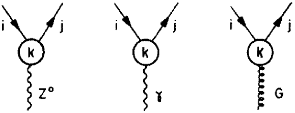
Figure 4: Penguin vertices

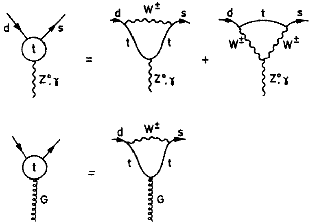
Figure 5: Penguin vertices resolved in terms of basic vertices

2.3.3 Effective Feynman Rules

With the help of the elementary vertices and propagators shown in figs. 2 and 3, one can now derive “Feynman rules” for the effective vertices discussed above by calculating simply the diagrams on the r.h.s. of the equations in figs. 5 and 7. These rules are given in the
’t Hooft–Feynman gauge as follows:

$${\rm Box}(\Delta S=2)~{}=~{}\lambda^{2}_{i}{{G^{2}_{\rm F}}\over{16\pi^{2}}}M_{\rm W}^{2}S_{0}(x_{i})(\bar{s}d)_{V-A}(\bar{s}d)_{V-A}$$ (2.15)

$${\rm Box}(T_{3}=-1/2)~{}=~{}\lambda_{i}{{G_{\rm F}}\over{\sqrt{2}}}{{\alpha}\over{2\pi\sin^{2}\Theta_{\rm W}}}B_{0}(x_{i})(\bar{s}d)_{V-A}(\bar{\mu}\mu)_{V-A}$$ (2.16)

$${\rm Box}(T_{3}=1/2)~{}=~{}\lambda_{i}{{G_{\rm F}}\over{\sqrt{2}}}{{\alpha}\over{2\pi\sin^{2}\Theta_{\rm W}}}[-4B_{0}(x_{i})](\bar{s}d)_{V-A}(\bar{\nu}\nu)_{V-A}$$ (2.17)

$$\bar{s}Zd~{}=~{}i\lambda_{i}{{G_{\rm F}}\over{\sqrt{2}}}{{e}\over{2\pi^{2}}}M^{2}_{Z}{{\cos\Theta_{\rm W}}\over{\sin\Theta_{\rm W}}}C_{0}(x_{i})\bar{s}\gamma_{\mu}(1-\gamma_{5})d$$ (2.18)

$$\bar{s}\gamma d~{}=~{}-i\lambda_{i}{{G_{\rm F}}\over{\sqrt{2}}}{{e}\over{8\pi^{2}}}D_{0}(x_{i})\bar{s}(q^{2}\gamma_{\mu}-q_{\mu}\not\!q)(1-\gamma_{5})d$$ (2.19)

$$\bar{s}G^{a}d~{}=~{}-i\lambda_{i}{{G_{\rm F}}\over{\sqrt{2}}}{{g_{s}}\over{8\pi^{2}}}E_{0}(x_{i})\bar{s}_{\alpha}(q^{2}\gamma_{\mu}-q_{\mu}\not\!q)(1-\gamma_{5})T^{a}_{\alpha\beta}d_{\beta}$$ (2.20)

$$\bar{s}\gamma^{\prime}b~{}=~{}i\bar{\lambda}_{i}{{G_{\rm F}}\over{\sqrt{2}}}{{e}\over{8\pi^{2}}}D^{\prime}_{0}(x_{i})\bar{s}[i\sigma_{\mu\lambda}q^{\lambda}[m_{b}(1+\gamma_{5})]]b$$ (2.21)

$$\bar{s}G^{\prime a}b~{}=~{}i\bar{\lambda}_{i}{{G_{\rm F}}\over{\sqrt{2}}}{{g_{s}}\over{8\pi^{2}}}E^{\prime}_{0}(x_{i})\bar{s}_{\alpha}[i\sigma_{\mu\lambda}q^{\lambda}[m_{b}(1+\gamma_{5})]]T^{a}_{\alpha\beta}b_{\beta}\,,$$ (2.22)

where $\lambda_{i}=V^{*}_{is}V_{id}$ and $\bar{\lambda}_{i}=V^{*}_{is}V_{ib}$. Here $q_{\mu}$ is the outgoing gluon or photon momentum. Moreover we have set $m_{s}=0$ in the last two rules. The rules in (2.15)-(2.22) correct for the correspoding rules given in [3] which contained unfortunately some misprints. Together with the rules of figs. 2 and 3 they allow the calculation of the effective Hamiltonians for FCNC processes without the inclusion of QCD corrections. To this end some care is needed. The penguin vertices should be used in the same way as the elementary vertices of fig. 3 and which follow from $i{\cal L}$. Once a mathematical expression corresponding to a given diagram has been found, the contribution of this diagram to the relevant effective Hamiltonian is obtained by multiplying this mathematical expression by “i”. On the other hand our conventions for the box vertices are such that they directly give the contributions to the effective Hamiltonians. We will give an example below by calculating the internal top contributions to $K^{+}\to\pi^{+}\nu\bar{\nu}$. First, however, we would like to make general remarks emphasizing the new features of these effective vertices as compared to the ones of fig. 1.:

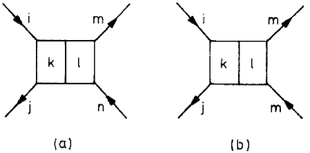
Figure 6: Box vertices

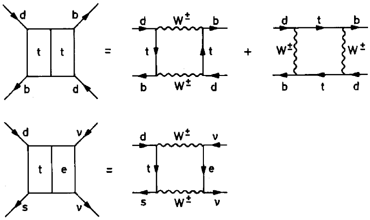
Figure 7: Box vertices resolved in terms of elementary vertices

• They are higher order in the gauge couplings and consequently suppressed relative to elementary transitions.

• Because of the internal $W^{\pm}$ exchanges all penguin vertices in fig. 5 are purely $V-A$, i.e. the effective vertices involving $\gamma$ and $G$ are parity violating as opposed to their elementary interactions in fig. 1! Also the structure of the $Z^{0}$ coupling changes since now only $V-A$ couplings are involved. The box vertices are of the $(V-A)\otimes(V-A)$ type.

• The effective vertices depend on the masses of internal quarks or leptons and consequently are calculable functions of

  $$x_{i}={{m_{i}^{2}}\over{M_{W}^{2}}},\qquad i=u,c,t.$$ (2.23)

  A set of basic universal functions can be found. These functions govern the physics of all FCNC processes. They are given below. The masses of internal leptons except for the $\tau$ contribution to $K^{+}\to\pi^{+}\nu\bar{\nu}$ can be set to zero.

• The effective vertices depend on elements of the CKM matrix and this dependence can be found directly from the diagrams of figs. 5 and 7.

• The dependence on external fermions manifests itself in two ways. First the CKM factors and the type of internal fermions depend on the external fermions considered. This in turn has an impact on the argument $x_{i}$ of the basic function and consequently on the strength of the vertex in question.

• The second dependence enters when one considers mass effects of external fermions. Since generally these masses are substantially smaller than $M_{W}$, it suffices to include this dependence to first order in $m_{\rm ext}/M_{W}$. In this case one can summarize the effects of $m_{\rm ext}$ by introducing new effective vertices without changing the structure of the vertices of figs. 5 and 7 which have been obtained by setting $m_{\rm ext}=0$. For all practical purposes only external mass effects in penguin diagrams need to be considered. The new vertices are then described as in fig. 8 where the cross indicates which external mass has been taken into account. These vertices are proportional to $m_{\rm ext}$, introduce new $x_{i}$ dependent functions and have different Dirac structure as seen in the last two rules of (2.15)-(2.22). They have, however, the same dependence on the CKM parameters as the corresponding vertices with $m_{\rm ext}=0$. It turns out that only the external mass effects in photonic and gluonic vertices are relevant.

• Another new feature of the effective vertices of figs. 5, 7 and 8 as compared with the elementary vertices is their dependence on the gauge used for the $W^{\pm}$ propagator. We will return to this point below.

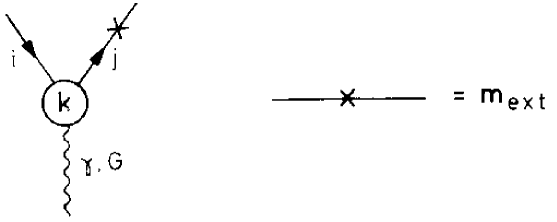
Figure 8: External mass in an effective penguin vertex (“magnetic penguin”)

2.3.4 Basic Functions

The basic functions present in (2.15)-(2.22) were calculated by various authors, in particular by Inami and Lim [18]. They are given explicitly as follows:

$$B_{0}(x_{t})={1\over 4}\left[{x_{t}\over{1-x_{t}}}+{{x_{t}\ln x_{t}}\over{(x_{t}-1)^{2}}}\right]$$ (2.24)

$$C_{0}(x_{t})={x_{t}\over 8}\left[{{x_{t}-6}\over{x_{t}-1}}+{{3x_{t}+2}\over{(x_{t}-1)^{2}}}\;\ln x_{t}\right]$$ (2.25)

$$D_{0}(x_{t})=-{4\over 9}\ln x_{t}+{{-19x_{t}^{3}+25x_{t}^{2}}\over{36(x_{t}-1)^{3}}}+{{x_{t}^{2}(5x_{t}^{2}-2x_{t}-6)}\over{18(x_{t}-1)^{4}}}\ln x_{t}$$ (2.26)

$$E_{0}(x_{t})=-{2\over 3}\ln x_{t}+{{x_{t}^{2}(15-16x_{t}+4x_{t}^{2})}\over{6(1-x_{t})^{4}}}\ln x_{t}+{{x_{t}(18-11x_{t}-x_{t}^{2})}\over{12(1-x_{t})^{3}}}$$ (2.27)

$$D^{\prime}_{0}(x_{t})=-{{(8x_{t}^{3}+5x_{t}^{2}-7x_{t})}\over{12(1-x_{t})^{3}}}+{{x_{t}^{2}(2-3x_{t})}\over{2(1-x_{t})^{4}}}\ln x_{t}$$ (2.28)

$$E^{\prime}_{0}(x_{t})=-{{x_{t}(x_{t}^{2}-5x_{t}-2)}\over{4(1-x_{t})^{3}}}+{3\over 2}{{x_{t}^{2}}\over{(1-x_{t})^{4}}}\ln x_{t}$$ (2.29)

$$S_{0}(x_{t})=\frac{4x_{t}-11x^{2}_{t}+x^{3}_{t}}{4(1-x_{t})^{2}}-\frac{3x^{3}_{t}\ln x_{t}}{2(1-x_{t})^{3}}$$ (2.30)

$$S_{0}(x_{c},x_{t})=x_{c}\left[\ln\frac{x_{t}}{x_{c}}-\frac{3x_{t}}{4(1-x_{t})}-\frac{3x^{2}_{t}\ln x_{t}}{4(1-x_{t})^{2}}\right]\,,$$ (2.31)

where in the last expression we keep only linear terms in $x_{c}\ll 1$, but of course all orders in $x_{t}$. The subscript “$0$” indicates that these functions do not include QCD corrections to the relevant penguin and box diagrams. These corrections will be discussed in subsequent sections.

The functions $D_{0}$ and $D^{\prime}_{0}$ given here are valid for internal up–type quarks. Denoting by $\tilde{D}_{0}$ and $\tilde{D}^{\prime}_{0}$ the corresponding functions involving internal down–type quarks, one has

$$\tilde{D}_{0}(x_{b})=D_{0}(x_{b})-E_{0}(x_{b});\quad\tilde{D}^{\prime}_{0}(x_{b})=D^{\prime}_{0}(x_{b})-E^{\prime}_{0}(x_{b}).$$ (2.32)

In writing the expressions in (2.24)-(2.31) we have omitted $x_{t}$–independent terms which do not contribute to decays due to the GIM mechanism. Moreover

$$S_{0}(x_{t})\equiv F(x_{t},x_{t})+F(x_{u},x_{u})-2F(x_{t},x_{u})$$ (2.33)

and

$$S_{0}(x_{i},x_{j})=F(x_{i},x_{j})+F(x_{u},x_{u})-F(x_{i},x_{u})-F(x_{j},x_{u}),$$ (2.34)

where $F(x_{i},x_{j})$ is the true function corresponding to the box diagram. In this way the effective Hamiltonian for $\Delta S=2$ transitions as given in section 4 can be directly obtained in the usual form by summing only over $t$ and $c$ quarks.

2.4 Effective Hamiltonians for FCNC Transitions and GIM Mechanism

With the help of the Feynman rules given in figs. 2 and 3 and in (2.15)-(2.22) it is an easy matter to construct an effective Hamiltonian for any FCNC process. As an example consider the decay $K^{+}\to\pi^{+}\bar{\nu}_{e}\nu_{e}$ to which the diagrams in fig. 9 contribute.

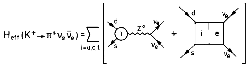
Figure 9: Calculation of ${\cal H}_{\rm eff}(K^{+}\to\pi^{+}\nu_{e}\bar{\nu}_{e})$

Replacing the $Z^{0}$ propagator by $ig_{\mu\nu}/M_{Z}^{2}$, using the rules of figs. 2 and 3 and (2.15)-(2.22), and multiplying the first diagram by “i”, we find the well-known result for the top contribution to this decay:

$${\cal H}_{\rm eff}(K^{+}\to\pi^{+}\nu_{e}\bar{\nu}_{e})={{G_{\rm F}}\over{\sqrt{2}}}\;{{\alpha}\over{2\pi\sin^{2}\Theta_{\rm W}}}\;V_{ts}^{*}V_{td}\;[C_{0}(x_{t})-4B_{0}(x_{t})]\;(\bar{s}d)_{V-A}(\bar{\nu}_{e}\nu_{e})_{V-A}.$$ (2.35)

For decays involving photonic and/or gluonic penguin vertices, the $1/q^{2}$ in the propagator cancels the $q^{2}$ in the vertex and the resulting effective Hamiltonian can again be written in terms of local four–fermion operators. Thus generally an effective Hamiltonian for any decay considered can be written in the absence of QCD corrections as

$${\cal H}_{\rm eff}^{\rm FCNC}=\sum_{k}C_{k}O_{k},$$ (2.36)

where $O_{k}$ denote local operators such as $(\bar{s}d)_{V-A}(\bar{s}d)_{V-A}$, $(\bar{s}d)_{V-A}(\bar{u}u)_{V-A}$ etc. The coefficients $C_{k}$ of these operators are simply linear combinations of the functions of eq. (2.24)-(2.31) times the corresponding CKM factors which can be read off from our rules. Later we will exhibit these CKM factors. The fact that the coefficients $C_{k}$ for any process considered can be expressed in terms of universal functions (2.24)-(2.31) demonstrates the usefulness of the formulation of FCNC decays in terms of effective vertices. We will encounter many examples of the expansion (2.36) in the course of this review.

At this stage it is useful to return to the GIM mechanism which did not allow tree level FCNC transitions. This mechanism is also felt in the Hamiltonian of (2.36) and in fact it is fully effective when the masses of internal quarks of a given charge are set to be equal, e.g. $m_{u}=m_{c}=m_{t}$. Indeed the CKM factors in any FCNC process enter in the combinations

$$C_{k}\propto\sum_{i=u,c,t}\lambda_{i}\;R(x_{i})~{}~{}~{}~{}{\rm or}~{}~{}~{}~{}\sum_{i,j=u,c,t}\lambda_{i}\lambda_{j}\;\tilde{R}(x_{i},x_{j}),$$ (2.37)

where $R,\tilde{R}$ denote any of the functions of (2.24)-(2.31), and the $\lambda_{i}$ are given in the case of $K$ and $B$ meson decays and particle–antiparticle mixing as follows:

$$\lambda_{i}=\cases{V_{is}^{*}V_{id}&~{}~{}~{}$K$--decays, ~{}~{}$K^{0}-\bar{K}^{0}$\cr V_{ib}^{*}V_{id}&~{}~{}~{}$B$--decays, ~{}~{}$B^{0}_{d}-\bar{B}^{0}_{d}$\cr V_{ib}^{*}V_{is}&~{}~{}~{}$B$--decays, ~{}~{}$B^{0}_{s}-\bar{B}^{0}_{s}$\cr}$$ (2.38)

They satisfy the unitarity relation

$$\lambda_{u}+\lambda_{c}+\lambda_{t}=0,$$ (2.39)

which implies vanishing coefficients $C_{k}$ in (2.37) if $x_{u}=x_{c}=x_{t}$. For this reason the mass–independent terms in the calculation of the basic functions in (2.24)-(2.31) can always be omitted. In this limit, FCNC decays and transitions are absent. Thus beyond tree level the conditions for a complete GIM cancellation of FCNC processes are:

• Unitarity of the CKM matrix

• Exact horizontal flavour symmetry which assures the equality of quark masses of a given charge.

It should be emphasized that such a horizontal symmetry is very natural, as the quantum numbers of all fermions of a given charge are equal in the Standard Model and so these fermions can be naturally put into multiplets of some horizontal symmetry group. Now in nature such a horizontal symmetry, even if it exists at very short distance scales, is certainly broken at low energies by the disparity of masses of quarks of a given charge. This in fact is the origin of the breakdown of the GIM mechanism at the one–loop level and the appearance of FCNC transitions. The size of this breakdown, and consequently the size of FCNC transitions, depends on the disparity of masses, on the behaviour of the basic functions of (2.24)-(2.31), and can be affected by QCD corrections as we will see below. Let us make two observations:

• For small $x_{i}\ll 1$, relevant for $i\not=t$, the functions (2.24)-(2.31) behave as follows:

  $$S_{0}(x_{i})\propto x_{i},\quad B_{0}(x_{i})\propto x_{i}\ln x_{i},\quad C_{0}(x_{i})\propto x_{i}\ln x_{i}$$ (2.40)

  $$D_{0}(x_{i})\propto\ln x_{i},\quad E_{0}(x_{i})\propto\ln x_{i},\quad D^{\prime}_{0}(x_{i})\propto x_{i},\quad E^{\prime}_{0}(x_{i})\propto x_{i}.$$ (2.41)

  This implies “hard” (quadratic) GIM suppression for processes governed by the functions $S,B,C,D^{\prime},E^{\prime}$ provided the top quark contributions due to small CKM factors can be neglected. In the case of $D(x_{i})$ and $E(x_{i})$ only “soft” (logarithmic) GIM suppression is present.

• For large $x_{t}$ we have

  $$S_{0}(x_{t})\propto x_{t},\quad B_{0}(x_{t})\propto{\rm const},\quad C_{0}(x_{t})\propto x_{t}$$ (2.42)

  $$D_{0}(x_{t})\propto\ln x_{t},\quad E_{0}(x_{t})\propto{\rm const},\quad D^{\prime}_{0}(x_{t})\propto{\rm const},\quad E^{\prime}_{0}(x_{t})\propto{\rm const}.$$ (2.43)

Thus for processes governed by top quark contributions, the GIM suppression is not effective at the one loop level and in fact in the case of decays and transitions receiving contributions from $S_{0}(x_{t})$ and $C_{0}(x_{t})$ some important enhancement is possible.

The latter property emphasizes the special role of $K$ and $B$ decays with regard to FCNC transitions. In these decays the appearance of the top quark in the internal loop with $m_{t}>M_{W}\gg m_{c},m_{u}$ removes the GIM suppression, making $K$ and $B$ decays a particularly useful place to test FCNC transitions and to study the physics of the top quark. Of course the hierarchy of various FCNC transitions is also determined by the hierarchy of the elements of the CKM matrix allowing this way to perform sensitive tests of this sector of the Standard Model.

The FCNC decays of $D$–mesons are much stronger suppressed because only $d$, $s$, and $b$ quarks with $m_{d},m_{s},m_{b}\ll M_{W}$ enter internal loops and the GIM mechanism is much more effective. Also the known structure of the CKM matrix is less favorable than in $K$ and $B$ decays. For these reasons we will restrict our presentation to the latter. In the extensions of the Standard Model, FCNC transitions are possible at the tree level and the hierarchies discussed here may not apply.

The formalism developed so far is not complete because it does not include QCD corrections. Moreover we did not address the classification of the local operators $O_{i}$ and we have not shown how to translate the calculations done in terms of quarks into predictions for the decays of their bound states, the hadrons. These issues will be the topics of the following subsection.

2.5 QCD, OPE and Renormalization Group

2.5.1 Preliminary Remarks

An amplitude for a decay of a given meson $M=K,B,\ldots\;$ into a final state $F$ is simply given by

$$A(M\to F)=\langle F\mid{\cal H}_{\rm eff}\mid M\rangle\,,$$ (2.44)

where ${\cal H}_{\rm eff}$ is the relevant Hamiltonian such as given in (2.36). Since all Hamiltonians considered can be written as linear combinations of local four–fermion operators, the result for the decay amplitude is generally given by

$$A(M\to F)=\sum_{i}C_{i}\langle F\mid O_{i}\mid M\rangle.$$ (2.45)

In the case of $B^{0}-\bar{B}^{0}$ mixing and $K^{0}-\bar{K}^{0}$ mixing, $\mid M\rangle$ and $\langle F\mid$ have to be changed appropriately.

Before further discussing (2.45) we have to elaborate on QCD corrections to weak decays. Clearly these decays originate in weak transitions mediated by $W^{\pm}$ and $Z^{0}$. However, the presence of strong and electromagnetic interactions often has an important impact on weak decays and consequently these interactions have a natural place in the physics of quark mixing, CP violation and rare decays. We have already seen the existence of FCNC transitions involving photonic and gluonic penguin diagrams. As far as electromagnetic interactions are concerned, it is sufficient to work to first order in $\alpha$. However, the case of strong interactions is very different and must be carefully investigated.

Due to the fact that $W^{\pm}$ and $Z^{0}$ are very massive, the basic weak transitions take place at very short distance scales ${\cal O}(1/M_{W,Z}^{2})$. The strong interactions being active at both short and long distances change this picture in the case of hadron decays, and generally weak decays of hadrons receive contributions from both short and long distances.

Now due to asymptotic freedom present in QCD, its effective coupling constant $\alpha_{s}(\mu)$ becomes small at $\mu=M_{W,Z}$. In the two loop approximation this running coupling constant is given by

$${{\alpha_{s}(\mu)}\over{4\pi}}={{\bar{g}^{2}_{s}(\mu)}\over{16\pi^{2}}}={{1}\over{\beta_{0}\ln(\mu^{2}/\Lambda^{2}_{\overline{MS}})}}-{{\beta_{1}}\over{\beta^{3}_{0}}}{{\ln\ln(\mu^{2}/\Lambda^{2}_{\overline{MS}})}\over{\ln^{2}(\mu^{2}/\Lambda^{2}_{\overline{MS}})}}\,,$$ (2.46)

where $\beta_{0}=(33-2f)/3$ and $\beta_{1}=(306-38f)/3$ with $f$ being the number of “effective” flavours. What “effective” means here will be explained below. Roughly speaking $f=6$ for $\mu\geq m_{\rm t}$, $f=5$ for $m_{\rm b}\leq\mu\leq m_{\rm t}$, $f=4$ for $m_{\rm c}\leq\mu\leq m_{\rm b}$ and $f=3$ for $\mu\leq m_{\rm c}$. $\Lambda_{\overline{MS}}$ is the QCD scale parameter [19] which generally depends on $f$. Denoting by $\alpha^{(f)}_{s}$ the effective coupling constant for a theory with $f$ effective flavours and by $\Lambda^{(f)}_{\overline{MS}}$ the corresponding QCD scale parameter, we have the following boundary conditions which follow from the continuity of $\alpha_{s}$:

$$\alpha_{s}^{(6)}(m_{\rm t})=\alpha_{s}^{(5)}(m_{\rm t}),\qquad\alpha_{s}^{(5)}(m_{\rm b})=\alpha_{s}^{(4)}(m_{\rm b}),\qquad\alpha_{s}^{(4)}(m_{\rm c})=\alpha_{s}^{(3)}(m_{\rm c}).$$ (2.47)

These conditions allow to find values of $\Lambda^{(f)}_{\overline{MS}}$ for different $f$ once one particular $\Lambda^{(f)}_{\overline{MS}}$ is known. In table 2 we show different $\alpha^{(f)}_{s}(\mu)$ and $\Lambda^{(f)}_{\overline{MS}}$ corresponding to

$$\alpha_{s}^{(5)}(M_{\rm Z})=0.118\pm 0.005,$$ (2.48)

which is in the ball park of the present world average extracted from different processes [20]. We observe that for $\mu\geq m_{\rm c}$ the values of $\alpha_{s}(\mu)$ are sufficiently small that the effects of strong interactions can be treated in perturbation theory. When one moves to low energy scales, $\alpha_{s}$ increases and at $\mu\approx{\cal O}(1~{}\,{\rm GeV})$ and high values of $\Lambda^{(3)}_{\overline{MS}}$ one finds $\alpha_{s}^{(3)}(\mu)>0.5$. This signals breakdown of perturbation theory for scales lower than $1~{}\,{\rm GeV}$. Yet it is gratifying that strong interaction contributions to weak decays coming from scales higher than $1~{}\,{\rm GeV}$ can be treated by perturbative methods.

$\alpha_{s}^{(6)}(m_{\rm t})$	$0.1037$	$0.1054$	$0.1079$	$0.1104$	$0.1120$
$\Lambda_{\overline{\rm MS}}^{(6)}[\,{\rm MeV}]$	$66$	$76$	$92$	$110$	$123$
$\alpha_{s}^{(5)}(M_{\rm Z})$	$0.113$	$0.115$	$0.118$	$0.121$	$0.123$
$\Lambda_{\overline{\rm MS}}^{(5)}[\,{\rm MeV}]$	$169$	$190$	$226$	$267$	$296$
$\alpha_{s}^{(5)}(m_{\rm b})$	$0.204$	$0.211$	$0.222$	$0.233$	$0.241$
$\Lambda_{\overline{\rm MS}}^{(4)}[\,{\rm MeV}]$	$251$	$278$	$325$	$376$	$413$
$\alpha_{s}^{(4)}(m_{\rm c})$	$0.336$	$0.357$	$0.396$	$0.443$	$0.482$
$\Lambda_{\overline{\rm MS}}^{(3)}[\,{\rm MeV}]$	$297$	$325$	$372$	$421$	$457$
$\alpha_{s}^{(3)}(1\,{\rm GeV})$	$0.409$	$0.444$	$0.514$	$0.605$	$0.690$

Table 2: Values of $\alpha^{(f)}_{s}(\mu)$ and $\Lambda^{(f)}_{\overline{MS}}$ corresponding to $\alpha_{s}^{(5)}(M_{\rm Z})=0.113$, 0.115, 0.118, 0.121, 0.123 with $m_{\rm c}=1.3~{}\,{\rm GeV}$, $m_{\rm b}=4.4~{}\,{\rm GeV}$ and $m_{\rm t}=170~{}\,{\rm GeV}$

The impact of QCD effects on weak decays depends crucially on the process considered, which is clearly seen when leptonic, semi–leptonic and non–leptonic decays are compared with each other.

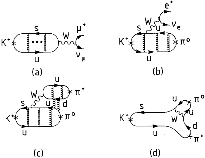
Figure 10: Examples of diagrams contributing to a) leptonic b) semi–leptonic and c,d) non–leptonic decays. The curly lines are gluons.

Consider for instance the leptonic decay $K^{+}\to\mu^{+}\nu_{\mu}$. One has (fig. 10a)

$$A(K^{+}\to\mu^{+}\nu_{\mu})={{G_{\rm F}}\over{\sqrt{2}}}V_{us}^{*}\;(\bar{\nu}_{\mu}\mu^{-})_{V-A}\;\langle 0\mid(\bar{s}u)_{V-A}\mid K^{+}\rangle.$$ (2.49)

Since gluons do not connect the lepton and quark currents, this factorized form of the amplitude (lepton current times the matrix element of the quark current) remains valid in the presence of strong interactions. In other words, cutting the $W$–propagator separates the diagram into two simpler subdiagrams. The full effect of strong interactions is then absorbed in the matrix element of the quark current. Since there are no loops involving simultaneously $W^{\pm}$ and gluons, and the $K$ mass is low, the strong interaction effects present in the current matrix element are purely long range and must be treated by non–perturbative methods. Yet the leptonic decays are the simplest ones because the effects of strong interactions can be fully absorbed in the current matrix elements. The latter are simple enough so that lattice calculations or QCD sum rules can give plausible estimates for their values. Moreover they can be determined experimentally. The knowledge of $\langle 0\mid(\bar{s}u)_{V-A}\mid K^{+}\rangle$ determines $F_{K}$ and the knowledge of analogous matrix elements fixes the decay constants of other mesons.

Semileptonic decays are slightly more complicated. However, the factorization of the amplitude into a lepton current and a matrix element of the relevant quark current remains also true here as seen in fig. 10b:

$$A(K^{+}\to\pi^{o}e^{+}\nu)={{G_{\rm F}}\over{\sqrt{2}}}V_{us}^{*}(\bar{\nu}_{e}e^{-})_{V-A}\langle\pi^{0}\mid(\bar{s}u)_{V-A}\mid K^{+}\rangle\,.$$ (2.50)

Again the strong interactions are compactly collected in the matrix element $\langle\pi^{0}\mid(\bar{s}u)_{V-A}\mid K^{+}\rangle$ which can in principle be extracted from experimental data or calculated by non–perturbative methods. Since this time the matrix element involves two meson states, its evaluation is more difficult and only on the border of lattice capabilities. For these reasons several models for these matrix elements have been invoked. Moreover, in the case of $K$ decays, chiral perturbation theory turns out to be useful. On the other hand, matrix elements involving $B$ mesons can be efficiently studied in the Heavy Quark Effective Theory. Furthermore, in inclusive semi–leptonic decays of heavy quarks QCD corrections resulting from real gluon emission can be calculated perturbatively. These issues are discussed by Neubert in a separate chapter in this book.

The non–leptonic decays such as $K\to\pi\pi$ or $B\to DK$ are more complicated to analyze and to calculate because the factorization of a given matrix element of a four–fermion operator into the product of current matrix elements is no longer true. Indeed now the gluons can connect the two quark currents (fig. 10c), and in addition the diagrams of fig. 10d contribute. The breakdown of factorization in non–leptonic decays is present both at short and long distances simply because the effects of strong interactions are felt both at large and small momenta. At large momenta, however, the QCD coupling constant is small and the non–factorizable contributions can be studied in perturbation theory. In order to accomplish this task, one has to separate first short distance effects from long distance effects. This is most elegantly done by means of the operator product expansion approach (OPE) combined with the renormalization group. In order to discuss these methods we have to say a few words about the effective field theory picture which underlies our discussion presented so far.

2.5.2 Effective Field Theory Picture

The basic framework for weak decays of hadrons containing $u$, $d$, $s$, $c$ and $b$ quarks is the effective field theory relevant for scales $\mu\ll M_{W},M_{Z},m_{t}$. This framework, as we have seen above, brings in local operators which govern “effectively” the transitions in question. From the point of view of the decaying hadrons containing the lightest five quarks this is the only correct picture we know and also the most efficient one for studying the presence of QCD. Furthermore it represents the generalization of the Fermi theory as formulated by Sudarshan and Marshak [21] and Feynman and Gell-Mann [22] forty years ago.

Indeed the simplest effective Hamiltonian without QCD effects that one would find from the first diagram of fig. 11 is (see (2.14))

$${\cal H}^{0}_{\rm eff}=\frac{G_{\rm F}}{\sqrt{2}}V_{cb}V_{cs}^{*}(\bar{c}b)_{V-A}(\bar{s}c)_{V-A}\,,$$ (2.51)

where $G_{\rm F}$ is the Fermi constant, $V_{ij}$ are the relevant CKM factors and

$$(\bar{c}b)_{V-A}(\bar{s}c)_{V-A}\equiv(\bar{c}\gamma_{\mu}(1-\gamma_{5})b)(\bar{s}\gamma_{\mu}(1-\gamma_{5})c)=Q_{2}$$ (2.52)

is a $(V-A)\cdot(V-A)$ current-current local operator usually denoted by $Q_{2}$. The situation in the Standard Model is, however, more complicated because of the presence of additional interactions which effectively generate new operators. These are in particular the gluon, photon and $Z^{0}$-boson exchanges and internal top contributions as we have seen above. Some of the elementary interactions of this type are shown this time for $B$ decays in fig. 11. Consequently the relevant effective Hamiltonian for $B$-meson decays involves generally several operators $Q_{i}$ with various colour and Dirac structures which are different from $Q_{2}$. Moreover each operator is multiplied by a calculable coefficient $C_{i}(\mu)$:

$${\cal H}_{\rm eff}=\frac{G_{\rm F}}{\sqrt{2}}V_{\rm CKM}\sum_{i}C_{i}(\mu)Q_{i},$$ (2.53)

where the scale $\mu$ is discussed below and $V_{\rm CKM}$ denotes the relevant CKM factor. Analogous expressions apply to $K$ and $D$ decays with an appropriate change of flavours.

At this stage it should be mentioned that the usual Feynman diagram drawings of the type shown in fig. 11 containing full $W$-propagators, $Z^{0}-$propagators and top-quark propagators represent really the happening at scales ${\cal O}(M_{\rm W})$ whereas the true picture of a decaying hadron is more correctly described by the local operators in question. Thus, whereas at scales ${\cal O}(M_{\rm W})$ we have to deal with the full six-quark theory containing the photon, weak gauge bosons and gluons, at scales ${\cal O}(1\,{\rm GeV})$ the relevant effective theory contains only three light quarks $u$, $d$ and $s$, gluons and the photon. At intermediate energy scales $\mu={\cal O}(m_{b})$ and $\mu={\cal O}(m_{c})$ relevant for beauty and charm decays, effective five-quark and effective four-quark theories have to be considered, respectively.

The usual procedure then is to start at a high energy scale ${\cal O}(M_{W})$ and consecutively integrate out the heavy degrees of freedom (heavy with respect to the relevant scale $\mu$) from explicitly appearing in the theory. The word “explicitly” is very essential here. The heavy fields did not disappear. Their effects are merely hidden in the effective gauge coupling constants, running masses and most importantly in the coefficients describing the “effective” strength of the operators at a given scale $\mu$, the Wilson coefficient functions $C_{i}(\mu)$.

2.5.3 OPE and Renormalization Group

The Operator Product Expansion (OPE) combined with the renormalization group approach can be regarded as a mathematical formulation of the picture outlined above. In this framework the amplitude for an exclusive decay $M\to F$ is written as

$$A(M\to F)=\frac{G_{\rm F}}{\sqrt{2}}V_{\rm CKM}\sum_{i}C_{i}(\mu)\langle F\mid Q_{i}(\mu)\mid M\rangle,$$ (2.54)

which generalizes (2.45) to include QCD corrections. $Q_{i}$ denote the local operators generated by QCD and electroweak interactions. $C_{i}(\mu)$ stand for the Wilson coefficient functions (c-numbers). The following comments should be made:

• The scale $\mu$ separates the physics contributions in the “short distance” contributions (corresponding to scales higher than $\mu$) contained in $C_{i}(\mu)$ and the “long distance” contributions (scales lower than $\mu$) contained in $\langle F\mid Q_{i}(\mu)\mid M\rangle$. By evolving the scale from $\mu={\cal O}(M_{W})$ down to lower values of $\mu$ one transforms the physics information at scales higher than $\mu$ from the hadronic matrix elements into $C_{i}(\mu)$. Since no information is lost this way the full amplitude cannot depend on $\mu$. This is the essence of the renormalization group equations which govern the evolution $(\mu-dependence)$ of $C_{i}(\mu)$. This $\mu$-dependence must be cancelled by the one present in $\langle Q_{i}(\mu)\rangle$. It should be stressed, however, that this cancellation generally involves many operators due to the operator mixing under renormalization.

• The set of basic operators entering the OPE and “driving” a given weak decay can be specified at short distances, i.e. without solving the difficult non–perturbative problem. Similarly the Wilson coefficient functions of these operators can be calculated by means of perturbative methods as long as $\mu$ is not too small, say $\mu\geq 1~{}\,{\rm GeV}$.

• In view of two vastly different scales entering the analysis ($M_{W}\gg\mu\approx{\cal O}(1-5\,{\rm GeV})$), the usual perturbative expansion has to be improved, however. Indeed large logarithms $(\ln M_{W}/\mu)$ multiplying $\alpha_{s}$ have to be resummed to all orders in $\alpha_{s}$ before a reliable estimate of the $C_{i}$ can be obtained. This can be done very efficiently by means of the renormalization group methods as will be discussed in a moment. The resulting “renormalization group improved” perturbative expansion for the $C_{i}$’s in terms of the effective QCD coupling of (2.46) does not involve large logarithms and is more reliable.

Let us then say a few words about the $\mu$ dependence of the Wilson coefficients which is governed by the renormalization group. Many more details can be found in a recent review [4].

The general expression for $C_{i}(\mu)$ is given by:

$$\vec{C}(\mu)=\hat{U}(\mu,M_{W})\vec{C}(M_{W}),$$ (2.55)

where $\vec{C}$ is a column vector built out of $C_{i}$’s. $\vec{C}(M_{W})$ are the initial conditions which depend on the short distance physics at high energy scales. In particular they depend on $m_{t}$ and are generally linear combinations of the basic functions in (2.24)-(2.31). $\hat{U}(\mu,M_{W})$, the evolution matrix, is given as

$$\hat{U}(\mu,M_{W})=T_{g}\exp\left[\int_{g(M_{W})}^{g(\mu)}{dg^{\prime}\frac{\hat{\gamma}^{T}(g^{\prime})}{\beta(g^{\prime})}}\right]$$ (2.56)

with $g=g_{s}$ denoting the QCD effective coupling constant. $T_{g}$ denotes the ordering in the coupling $g$ so that the couplings increase from right to left (see (2.59)). $\beta(g)$ governs the evolution of $g$ and $\hat{\gamma}$ is the anomalous dimension matrix of the operators involved. The structure of this equation makes it clear that the renormalization group approach goes beyond usual perturbation theory. Indeed $\hat{U}(\mu,M_{W})$ sums automatically large logarithms $\log(M_{W}/\mu)$ which appear for $\mu<<M_{W}$. In the so-called leading logarithmic approximation (LO) terms $(g^{2}\log M_{W}/\mu)^{n}$ are summed. The next-to-leading logarithmic correction (NLO) to this result involves summation of terms $(g^{2})^{n}(\log M_{W}/\mu)^{n-1}$ and so on. This hierarchic structure gives the renormalization group improved perturbation theory.

As an example let us consider only QCD effects and the case of a single operator so that (2.55) reduces to

$$C(\mu)=U(\mu,M_{W})C(M_{W}),$$ (2.57)

where $C(\mu)$ denotes the coefficient of the operator in question. Keeping the first two terms in the expansions of $\gamma(g)$ and $\beta(g)$ in powers of $g$:

$$\gamma(g)=\gamma^{(0)}\frac{\alpha_{s}}{4\pi}+\gamma^{(1)}\frac{\alpha^{2}_{s}}{16\pi^{2}}\quad,\quad\beta(g)=-\beta_{0}\frac{g^{3}}{16\pi^{2}}-\beta_{1}\frac{g^{5}}{(16\pi^{2})^{2}}$$ (2.58)

and inserting these expansions into (2.56) gives

$$U(\mu,M_{\rm W})=\Biggl{[}1+{{\alpha_{s}(\mu)}\over{4\pi}}J\Biggl{]}\Biggl{[}{{\alpha_{s}(M_{W})}\over{\alpha_{s}(\mu)}}\Biggl{]}^{P}\Biggl{[}1-{{\alpha_{s}(M_{W})}\over{4\pi}}J\Biggl{]},$$ (2.59)

where

$$P={{\gamma^{(0)}}\over{2\beta_{0}}},~{}~{}~{}~{}~{}~{}~{}~{}~{}J={{P}\over{\beta_{0}}}\beta_{1}-{{\gamma^{(1)}}\over{2\beta_{0}}}.$$ (2.60)

General formulae for $\hat{U}(\mu,M_{W})$ in the case of operator mixing and valid also for electroweak effects can be found in [4, 23]. The leading logarithmic approximation corresponds to setting $J=0$ in (2.59) and dropping the second term in (2.46).

At this stage we should say a few words about the renormalization scheme dependence. The initial conditions $C(M_{\rm W})$ depend at the NLO level on the renormalization scheme for operators. Similarly NLO corrections in $U(\mu,M_{\rm W})$, represented by $J$ in (2.59), are scheme dependent through the scheme dependence of the two-loop anomalous dimensions $\gamma^{(1)}$. The scheme dependence in the last factor in (2.59) is cancelled by the scheme dependence of $C(M_{\rm W})$ and the scheme dependence of $C(\mu)$ is entirely given by the first factor in (2.59). This scheme dependence is cancelled by the one present in the matrix element $\langle F|Q_{i}(\mu)|M\rangle$ so that the resulting physical amplitudes are scheme independent.

In this review we will entirely work in the $\overline{MS}$ renormalization scheme and the only scheme dependence will be signalled by two different treatments of $\gamma_{5}$ in $D\not=4$ dimensions:

• NDR-scheme: anti-commuting $\gamma_{5}$

• HV-scheme: non-anti-commuting $\gamma_{5}$ [24]

Details of these schemes are discussed in [34, 25].

Clearly in order to calculate the full amplitude (2.54) also the hadronic matrix elements $\langle F|Q_{i}(\mu)|M\rangle$ have to be evaluated. Since they involve long distance contributions one is forced in this case to use non-perturbative methods such as lattice calculations, the $1/N$ expansion, QCD sum rules or chiral perturbation theory. In the case of semi-leptonic $B$ meson decays also the Heavy Quark Effective Theory (HQET) turns out to be a useful tool. In HQET the matrix elements are evaluated approximately in an expansion in $1/m_{b}$. Potential uncertainties in the calculation of the non-leading terms in this expansion have been stressed recently [26]. Needless to say, all these non-perturbative methods have some limitations. Consequently the dominant theoretical uncertainties in the decay amplitudes reside in the matrix elements of $Q_{i}$.

Figure 11: Typical Penguin and Box Diagrams.

2.5.4 Classification of Operators

Let us next systematically classify the operators which will appear in the subsequent sections of this review and which play the dominant role in the phenomenology of weak decays. Typical diagrams in the full theory from which these operators originate are indicated and shown in fig. 11. The cross in fig. 11d indicates as in fig. 8 that magnetic penguins originate from the mass-term on the external line in the usual QCD or QED penguin diagrams. The six classes are given as follows ($\alpha$ and $\beta$ are colour indices):

Current–Current (fig. 11a):

$$Q_{1}=(\bar{c}_{\alpha}b_{\beta})_{V-A}\;(\bar{s}_{\beta}c_{\alpha})_{V-A}~{}~{}~{}~{}~{}~{}Q_{2}=(\bar{c}b)_{V-A}\;(\bar{s}c)_{V-A}$$ (2.61)

QCD–Penguins (fig. 11b):

$$Q_{3}=(\bar{s}b)_{V-A}\sum_{q=u,d,s,c,b}(\bar{q}q)_{V-A}~{}~{}~{}~{}~{}~{}Q_{4}=(\bar{s}_{\alpha}b_{\beta})_{V-A}\sum_{q=u,d,s,c,b}(\bar{q}_{\beta}q_{\alpha})_{V-A}$$ (2.62)

$$Q_{5}=(\bar{s}b)_{V-A}\sum_{q=u,d,s,c,b}(\bar{q}q)_{V+A}~{}~{}~{}~{}~{}Q_{6}=(\bar{s}_{\alpha}b_{\beta})_{V-A}\sum_{q=u,d,s,c,b}(\bar{q}_{\beta}q_{\alpha})_{V+A}$$ (2.63)

Electroweak–Penguins (fig. 11c):

$$Q_{7}={3\over 2}\;(\bar{s}b)_{V-A}\sum_{q=u,d,s,c,b}e_{q}\;(\bar{q}q)_{V+A}~{}~{}~{}~{}~{}Q_{8}={3\over 2}\;(\bar{s}_{\alpha}b_{\beta})_{V-A}\sum_{q=u,d,s,c,b}e_{q}(\bar{q}_{\beta}q_{\alpha})_{V+A}$$ (2.64)

$$Q_{9}={3\over 2}\;(\bar{s}b)_{V-A}\sum_{q=u,d,s,c,b}e_{q}(\bar{q}q)_{V-A}~{}~{}~{}~{}~{}Q_{10}={3\over 2}\;(\bar{s}_{\alpha}b_{\beta})_{V-A}\sum_{q=u,d,s,c,b}e_{q}\;(\bar{q}_{\beta}q_{\alpha})_{V-A}$$ (2.65)

Magnetic–Penguins (fig. 11d):

$$Q_{7\gamma}=\frac{e}{8\pi^{2}}m_{b}\bar{s}_{\alpha}\sigma^{\mu\nu}(1+\gamma_{5})b_{\alpha}F_{\mu\nu}\qquad Q_{8G}=\frac{g}{8\pi^{2}}m_{b}\bar{s}_{\alpha}\sigma^{\mu\nu}(1+\gamma_{5})T^{a}_{\alpha\beta}b_{\beta}G^{a}_{\mu\nu}$$ (2.66)

$\Delta S=2$ and $\Delta B=2$ Operators (fig. 11e):

$$Q(\Delta S=2)=(\bar{s}d)_{V-A}(\bar{s}d)_{V-A}~{}~{}~{}~{}~{}Q(\Delta B=2)=(\bar{b}d)_{V-A}(\bar{b}d)_{V-A}$$ (2.67)

Semi–Leptonic Operators (fig. 11f):

$$Q_{9V}=(\bar{s}b)_{V-A}(\bar{\mu}\mu)_{V}~{}~{}~{}~{}~{}Q_{10A}=(\bar{s}b)_{V-A}(\bar{\mu}\mu)_{A}$$ (2.68)

$$Q_{\nu\bar{\nu}}=(\bar{s}b)_{V-A}(\bar{\nu}\nu)_{V-A}~{}~{}~{}~{}~{}Q_{\mu\bar{\mu}}=(\bar{s}b)_{V-A}(\bar{\mu}\mu)_{V-A}$$ (2.69)

The above set of operators is characteristic for any consideration of the interplay of QCD and electroweak effects, although, as we shall see in later chapters, on many occasions contributions of certain operators can be safely neglected. Moreover the set of operators $Q_{1}-Q_{10}$ given above has the flavours relevant for $B$ decays. In $K$ decays the operators $Q_{1}$ and $Q_{2}$ should be replaced by

$$Q_{1}=(\bar{s}_{\alpha}u_{\beta})_{V-A}\;(\bar{u}_{\beta}d_{\alpha})_{V-A}~{}~{}~{}~{}~{}~{}Q_{2}=(\bar{s}u)_{V-A}\;(\bar{u}d)_{V-A}.$$ (2.70)

The relevant operators $Q_{3}-Q_{10}$ are then found by simply replacing “$b$” by “$d$” and summing only over $q=u,d,s$ in (2.62)–(2.65). Similarly “$b$” has to be replaced by “$d$” in (2.68) and (2.69).

2.6 Manifestly Gauge Independent Formulation of FCNC Transitions

Let us return to the basic functions in (2.24)-(2.31). The expressions given there for the functions $B_{0}(x_{t})$, $C_{0}(x_{t})$ and $D_{0}(x_{t})$ correspond to the ’t Hooft–Feynman gauge ($\xi=1$). In an arbitrary $R_{\xi}$ gauge, these functions are generalized as follows [18]:

$$B_{0}(x_{t},\xi,T_{3})=\cases{B_{0}(x_{t})+{1\over 8}\bar{\varrho}(x_{t},\xi),&~{}~{}~{}~{}$T_{3}=1/2$;\cr B_{0}(x_{t})+{1\over 2}\bar{\varrho}(x_{t},\xi),&~{}~{}~{}~{}$T_{3}=-1/2$;\cr}$$ (2.71)

$$C_{0}(x_{t},\xi)=C_{0}(x_{t})+{1\over 2}\bar{\varrho}(x_{t},\xi)$$ (2.72)

$$D_{0}(x_{t},\xi)=D_{0}(x_{t})-2\bar{\varrho}(x_{t},\xi),$$ (2.73)

where $\bar{\varrho}(x_{t},\xi)$ summarizes the gauge dependence with $\bar{\varrho}(x_{t},1)=0$. Explicit formulae for $\bar{\varrho}(x_{t},\xi)$ can be found in [18, 9]. In (2.71), $T_{3}$ denotes the weak isospin of the outgoing fermions in the flavour conserving part of the box vertex. We observe that the $x_{t}$ dependence of the box vertices depends generally on $T_{3}$ in the flavour conserving part and only for $\xi=1$ it reduces to the single function $B_{0}(x_{t})$.

Now the initial conditions for the Wilson coefficient functions $C_{j}(M_{W})$ are generally given as linear combinations of the basic functions in (2.24)-(2.31). Since physical amplitudes cannot depend on the chosen gauge the basic functions have to enter $C_{j}(M_{W})$ in some special combinations which are gauge independent. These special linear combinations turn out to be as follows [9]:

$$C_{0}(x_{t},\xi)-4B_{0}(x_{t},\xi,1/2)=C_{0}(x_{t})-4B_{0}(x_{t})=X_{0}(x_{t})$$ (2.74)

$$C_{0}(x_{t},\xi)-B_{0}(x_{t},\xi,-1/2)=C_{0}(x_{t})-B_{0}(x_{t})=Y_{0}(x_{t})$$ (2.75)

$$C_{0}(x_{t},\xi)+{1\over 4}D_{0}(x_{t},\xi)=C_{0}(x_{t})+{1\over 4}D_{0}(x_{t})=Z_{0}(x_{t}).$$ (2.76)

Explicitly then:

$$X_{0}(x_{t})={{x_{t}}\over{8}}\;\left[{{x_{t}+2}\over{x_{t}-1}}+{{3x_{t}-6}\over{(x_{t}-1)^{2}}}\;\ln x_{t}\right]$$ (2.77)

$$Y_{0}(x_{t})={{x_{t}}\over 8}\;\left[{{x_{t}-4}\over{x_{t}-1}}+{{3x_{t}}\over{(x_{t}-1)^{2}}}\ln x_{t}\right]$$ (2.78)

$$Z_{0}(x_{t})=-{1\over 9}\ln x_{t}+{{18x_{t}^{4}-163x_{t}^{3}+259x_{t}^{2}-108x_{t}}\over{144(x_{t}-1)^{3}}}+{{32x_{t}^{4}-38x_{t}^{3}-15x_{t}^{2}+18x_{t}}\over{72(x_{t}-1)^{4}}}\ln x_{t}.$$ (2.79)

It is also found that the functions $X_{0},Y_{0},Z_{0}$ multiply always local operators of a particular structure (here $u$ represents $u,c,t$; $e$ represents $e,\mu,\tau$ etc.):

$S_{0}(x_{t})$:	$(\bar{s}d)_{V-A}(\bar{s}d)_{V-A}$
$X_{0}(x_{t})$:	$(\bar{s}d)_{V-A}(\bar{u}u)_{V-A},~{}~{}(\bar{s}d)_{V-A}(\bar{\nu}\nu)_{V-A}$
$Y_{0}(x_{t})$:	$(\bar{s}d)_{V-A}(\bar{d}d)_{V-A},~{}~{}(\bar{s}d)_{V-A}(\bar{e}e)_{V-A}$
$Z_{0}(x_{t})$:	$(\bar{s}d)_{V-A}(\bar{u}u)_{V},~{}~{}(\bar{s}d)_{V-A}(\bar{d}d)_{V},~{}~{}(\bar{s}d)_{V-A}(\bar{e}e)_{V}$
$E_{0}(x_{t})$:	$(\bar{s}d)_{V-A}(\bar{q}q)_{V},~{}~{}(\bar{s}_{\alpha}d_{\beta})_{V-A}(\bar{q}_{\beta}q_{\alpha})_{V}$
$D^{\prime}_{0}(x_{t})$:	$\bar{s}_{\alpha}\sigma^{\mu\nu}(1+\gamma_{5})b_{\alpha}F_{\mu\nu}$
$E^{\prime}_{0}(x_{t})$:	$\bar{s}_{\alpha}\sigma^{\mu\nu}T^{a}_{\alpha\beta}(1+\gamma_{5})b_{\beta}G^{a}_{\mu\nu}$

Here $\alpha$ and $\beta$ are colour indices, $F_{\mu\nu}$ is the electromagnetic field strength tensor and $G^{a}_{\mu\nu}$ the gluonic field strength tensor.

We note that $X_{0}(x_{t})$ and $Y_{0}(x_{t})$ are linear combinations of the $V-A$ components of $Z^{0}$–penguin and box–diagrams with final quarks or leptons having weak isospin $T_{3}$ equal to 1/2 and – 1/2, respectively. $Z_{0}(x_{t})$ is a linear combination of the vector component of the $Z^{0}$–penguin and the $\gamma$–penguin.

2.7 Penguin–Box Expansion for FCNC Processes

Having the set of gauge independet basic functions

$$S_{0}(x_{t}),\quad X_{0}(x_{t}),\quad Y_{0}(x_{t}),\quad Z_{0}(x_{t}),\quad E_{0}(x_{t}),\quad D^{\prime}_{0}(x_{t}),\quad E^{\prime}_{0}(x_{t})$$ (2.80)

at hand, let us return to the formal expression (2.54) and rewrite it in the form

$$A(M\to F)=\frac{G_{\rm F}}{\sqrt{2}}V_{\rm CKM}\sum_{i,k}\langle F\mid O_{k}(\mu)\mid M\rangle\;U_{kj}\;(\mu,M_{W})\;C_{j}(M_{W}),$$ (2.81)

where $U_{kj}(\mu,M_{W})$ is the renormalization group transformation from $M_{W}$ down to $\mu$ given in (2.56).

Now prior to the discussion of QCD effects we have formulated the FCNC decays in terms of effective vertices. This formulation demonstrates explicitly the universal character of short distance interactions and exhibits very clearly the dependence on internal quark masses, in particular $m_{t}$, given by the process independent functions (2.80). Yet as we have seen above, this universality and the transparent picture seems to have been lost after the inclusion of QCD effects because these effects are very different for different processes. Indeed when the analysis is done in the framework of OPE, the basic functions of (2.80) enter only the initial conditions of the renormalization group analysis, i.e. the presence of effective vertices is only felt in $C_{j}(M_{W})$. The correspondence between $C_{j}(M_{W})$ and the effective vertices is, however, not simple because generally a given diagram and the corresponding function contributes to several coefficient functions of local operators and the $C_{j}(M_{W})$ are just linear combinations of them. Moreover, since the transformation described by $\hat{U}(\mu,M_{W})$ is very complicated for non–leptonic decays, but very simple for semi–leptonic decays, the resulting amplitudes have no similarities. Indeed in the usual OPE analysis the amplitude (2.81) is rewritten as in (2.54). Thus, although the resulting coefficient functions evaluated at $\mu={\cal O}(1\,{\rm GeV})$ remember the $m_{t}$ dependence acquired through the effective vertices or basic functions, this dependence is hidden in a complicated numerical evaluation of $U_{jk}$. In other words, the $m_{t}$ dependence of a given effective vertex is distributed among various Wilson coefficient functions.

For phenomenological applications it is more elegant and more convenient to have a formalism in which the final formulae for all amplitudes are given explicitly in terms of the basic $m_{t}$-dependent functions discussed above.

In [9] an approach was presented which accomplishes this task. It gives the decay amplitudes as linear combinations of the basic, universal, process independent but $m_{t}$-dependent functions $F_{r}(x_{t})$ of (2.80) with corresponding coefficients $P_{r}$ characteristic for the decay under consideration. This approach termed “Penguin Box Expansion” (PBE) has the following general form:

$$A({\rm decay})=P_{0}({\rm decay})+\sum_{r}P_{r}({\rm decay})\,F_{r}(x_{t}),$$ (2.82)

where the sum runs over all possible functions contributing to a given amplitude. In (2.82) we have separated a $m_{t}$-independent term $P_{0}$ which summarizes contributions stemming from internal quarks other than the top, in particular the charm quark.

Many examples of PBE appear in this review. Several decays or transitions depend only on a single function out of the complete set (2.80). For completeness we give here the correspondence between various processes and the basic functions:

$B^{0}-\bar{B}^{0}$-mixing		$S_{0}(x_{t})$
$K\to\pi\nu\bar{\nu}$, $B\to X_{d,s}\nu\bar{\nu}$		$X_{0}(x_{t})$
$K\to\mu\bar{\mu}$, $B\to l\bar{l}$		$Y_{0}(x_{t})$
$K_{\rm L}\to\pi^{0}e^{+}e^{-}$		$Y_{0}(x_{t})$, $Z_{0}(x_{t})$, $E_{0}(x_{t})$
$\varepsilon^{\prime}$		$X_{0}(x_{t})$, $Y_{0}(x_{t})$, $Z_{0}(x_{t})$, $E_{0}(x_{t})$
$B\to X_{s}\gamma$		$D^{\prime}_{0}(x_{t})$, $E^{\prime}_{0}(x_{t})$
$B\to X_{s}\mu^{+}\mu^{-}$		$Y_{0}(x_{t})$, $Z_{0}(x_{t})$, $E_{0}(x_{t})$, $D^{\prime}_{0}(x_{t})$, $E^{\prime}_{0}(x_{t})$

In [9] an explicit transformation from OPE to PBE has been made. This transformation and the relation between these two expansions can be very clearly seen on the basis of (2.81). As we have seen, OPE puts the last two factors in this formula together, mixing this way the physics around $M_{W}$ with all physical contributions down to very low energy scales. The PBE is realized on the other hand by putting the first two factors together and rewriting $C_{j}(M_{W})$ in terms of the basic functions (2.80). This results in the expansion of (2.82). Further technical details and the methods for the evaluation of the coefficients $P_{r}$ can be found in [9], where further virtues of PBE are discussed.

Finally, we give approximate formulae having power-like dependence on $x_{t}$ for the basic, gauge independent functions of PBE:

$$S_{0}(x_{t})=0.784~{}x_{t}^{0.76},~{}~{}~{}~{}X_{0}(x_{t})=0.660~{}x_{t}^{0.575},$$ (2.83)

$$Y_{0}(x_{t})=0.315~{}x_{t}^{0.78},\quad Z_{0}(x_{t})=0.175~{}x_{t}^{0.93},\quad E_{0}(x_{t})=0.564~{}x_{t}^{-0.51},$$ (2.84)

$$D^{\prime}_{0}(x_{t})=0.244~{}x_{t}^{0.30},~{}~{}~{}~{}~{}~{}~{}~{}~{}~{}E^{\prime}_{0}(x_{t})=0.145~{}x_{t}^{0.19}.$$ (2.85)

In the range $150\,{\rm GeV}\leq m_{t}\leq 200\,{\rm GeV}$ these approximations reproduce the exact expressions to an accuracy better than 1%.

2.8 Inclusive Decays

So far we have discussed only exclusive decays. During recent years considerable progress has been made for inclusive decays of heavy mesons. The starting point is again the effective Hamiltonian in (2.53) which includes the short distance QCD effects in $C_{i}(\mu)$. The actual decay described by the operators $Q_{i}$ is then calculated in the spectator model corrected for additional virtual and real gluon corrections. Support for this approximation comes from heavy quark ($1/m_{b}$) expansions (HQE). Indeed the spectator model has been shown to correspond to the leading order approximation in the $1/m_{b}$ expansion. The next corrections appear at the ${\cal O}(1/m_{b}^{2})$ level. The latter terms have been studied by several authors [27, 28, 29] with the result that they affect various branching ratios by less than $10\%$ and often by only a few percent. There is a vast literature on this subject and we can only refer here to a few papers [29, 30] where further references can be found. Of particular importance for this field was also the issue of the renormalons which is nicely discussed in [31, 32].

XXXXXXXX Decay	Reference
$\Delta F=1$ Decays
current-current operators	[33, 34]
QCD penguin operators	[35, 23, 37, 38]
electroweak penguin operators	[36, 23, 37, 38]
magnetic penguin operators	[39, 54, 57, 58]
$Br(B)_{SL}$	[33, 40, 41]
inclusive $\Delta S=1$ decays	[42]
Particle-Antiparticle Mixing
$\eta_{1}$	[43]
$\eta_{2},~{}\eta_{B}$	[44]
$\eta_{3}$	[45]
Rare $K$- and $B$-Meson Decays
$K^{0}_{L}\rightarrow\pi^{0}\nu\bar{\nu}$, $B\rightarrow l^{+}l^{-}$, $B\rightarrow X_{\rm s}\nu\bar{\nu}$	[46, 47]
$K^{+}\rightarrow\pi^{+}\nu\bar{\nu}$, $K_{\rm L}\rightarrow\mu^{+}\mu^{-}$	[48]
$K^{+}\to\pi^{+}\mu\bar{\mu}$	[49]
$K_{\rm L}\rightarrow\pi^{0}e^{+}e^{-}$	[50]
$B\rightarrow X_{s}\mu^{+}\mu^{-}$	[51, 52]
$B\rightarrow X_{s}\gamma$	[53, 54, 55, 56, 57, 58]

Table 3: References to NLO Calculations

2.9 Weak Decays Beyond Leading Logarithms

Until 1989 most of the calculations in the field of weak decays were done in the leading logarithmic approximation. An exception was the important work of Altarelli et al. [33] who calculated NLO QCD corrections to the Wilson coefficients of the current-current operators in 1981. Today the effective Hamiltonians for weak decays are available at the next-to-leading level for the most important and interesting cases due to a series of publications devoted to this enterprise written during the last six years. The list of the existing calculations is given in table 3. We will discuss some of the entries in this list below. A detailed review of the existing NLO calculations is given in [4].

Let us recall why NLO calculations are important for the phenomenology of weak decays:

• The NLO is first of all necessary to test the validity of renormalization group improved perturbation theory.

• Without going to NLO the QCD scale $\Lambda_{\overline{MS}}$ extracted from various high energy processes cannot be used meaningfully in weak decays.

• Due to renormalization group invariance the physical amplitudes do not depend on the scales $\mu$ present in $\alpha_{s}$ or in the running quark masses, in particular $m_{t}(\mu)$, $m_{b}(\mu)$ and $m_{c}(\mu)$. However, in perturbation theory this property is broken through the truncation of the perturbative series. Consequently one finds sizable scale ambiguities in the leading order, which can be reduced considerably by going to NLO.

• In several cases the central issue of the top quark mass dependence is strictly a NLO effect.

3 Quark Mixing Matrix

3.1 General Remarks

Let us next discuss the stucture of the quark-mixing-matrix $\hat{V}$ defined by (2.12) in more detail. In the case of $N$ generations, this matrix is given by a unitary $N\times N$ matrix. The phase structure of the quark-mixing-matrix is not unique since we have the freedom of performing the following phase-transformations which are related to phase-transformations of the corresponding quark fields:

$$V_{ij}\to\exp(i\xi_{i})V_{ij}\exp(-i\tilde{\xi}_{j}).$$ (3.1)

Note that there is no summation over the quark-flavour indices $i$ and $j$ in this equation. Using the transformations (3.1), it can be shown that the general $N$ generation quark-mixing-matrix is described by $(N-1)^{2}$ parameters consisting of

$$\frac{1}{2}N(N-1)$$ (3.2)

Euler-type angles and

$$\frac{1}{2}(N-1)(N-2)$$ (3.3)

complex phases.

Consequently the quark-mixing-matrix is real in the two-generation case and takes the following standard form [1, 17]:

$$\hat{V}_{\mbox{{\scriptsize C}}}=\left(\begin{array}[]{cc}\cos\theta_{\mbox{{\scriptsize C}}}&\sin\theta_{\mbox{{\scriptsize C}}}\\ -\sin\theta_{\mbox{{\scriptsize C}}}&\cos\theta_{\mbox{{\scriptsize C}}}\end{array}\right),$$ (3.4)

where $\sin\theta_{\mbox{{\scriptsize C}}}$ can be determined from semi-leptonic $K$-meson decays of the type $K\to\pi e^{+}\nu_{e}$ and is given by $\sin\theta_{\mbox{{\scriptsize C}}}=0.22$.

On the other hand the $3\times 3$ quark-mixing-matrix of the three generation Standard Model – the Cabibbo–Kobayashi–Maskawa–matrix (CKM matrix) [2] – is parametrized by three angles and a single complex phase. This phase leading to an imaginary part of the CKM matrix is a necessary ingredient to describe CP violation within the framework of the Standard Model.

Many parametrizations of the CKM matrix have been proposed in the literature. We will use two parametrizations in this review: the standard parametrization [59] recommended by the particle data group [60] and the Wolfenstein parametrization [62].

3.2 Standard Parametrization

Let us introduce the notation $c_{ij}=\cos\theta_{ij}$ and $s_{ij}=\sin\theta_{ij}$ with $i$ and $j$ being generation labels ($i,j=1,2,3$). The standard parametrization is then given as follows [60]:

$$V=\left(\begin{array}[]{ccc}c_{12}c_{13}&s_{12}c_{13}&s_{13}e^{-i\delta}\\ -s_{12}c_{23}-c_{12}s_{23}s_{13}e^{i\delta}&c_{12}c_{23}-s_{12}s_{23}s_{13}e^{i\delta}&s_{23}c_{13}\\ s_{12}s_{23}-c_{12}c_{23}s_{13}e^{i\delta}&-s_{23}c_{12}-s_{12}c_{23}s_{13}e^{i\delta}&c_{23}c_{13}\end{array}\right)\,,$$ (3.5)

where $\delta$ is the phase necessary for CP violation. $c_{ij}$ and $s_{ij}$ can all be chosen to be positive and $\delta$ may vary in the range $0\leq\delta\leq 2\pi$. However, the measurements of CP violation in $K$ decays force $\delta$ to be in the range $0<\delta<\pi$.

The extensive phenomenology of the last years has shown that $s_{13}$ and $s_{23}$ are small numbers: ${\cal O}(10^{-3})$ and ${\cal O}(10^{-2})$, respectively. Consequently to an excellent accuracy $c_{13}=c_{23}=1$ and the four independent parameters are given as

$$s_{12}=|V_{us}|,\quad s_{13}=|V_{ub}|,\quad s_{23}=|V_{cb}|,\quad\delta$$ (3.6)

with the phase $\delta$ extracted from CP violating transitions or loop processes sensitive to $|V_{td}|$. The latter fact is based on the observation that for $0\leq\delta\leq\pi$, as required by the analysis of CP violation in the $K$ system, there is a one–to–one correspondence between $\delta$ and $|V_{td}|$ given by

$$|V_{td}|=\sqrt{a^{2}+b^{2}-2ab\cos\delta},\qquad a=|V_{cd}V_{cb}|,\qquad b=|V_{ud}V_{ub}|\,.$$ (3.7)

What are the phenomenological advantages of (3.5) [61]?

• $|V_{ub}|$ is given by a single angle which is known to be very small. Therefore $V_{ud},V_{us},V_{cb}$ and $V_{tb}$ are also given each by a single parameter to an approximation better than four significant figures. The relation between parameters and experimentally measured quantities gets hence extremely simple.

• Each of the angles may then be characterized by a single physical process, e.g. $\theta_{23}$ is directly measured by the $b\to c$ transition.

• The CP violating phase is always multiplied by the very small $s_{13}$. This shows clearly the suppression of CP violation.

For numerical evaluations the use of the standard parametrization is strongly recommended. However once the four parameters in (3.6) have been determined it is often useful to make a change of basic parameters in order to see the structure of the result more transparently. This brings us to the Wolfenstein parametrization [62] and its generalization given in [63].

3.3 Wolfenstein Parameterization Beyond Leading Order

The original Wolfenstein parametrization [62] is an approximate parametrization of the CKM matrix in which each element is expanded as a power series in the small parameter $\lambda=|V_{us}|=0.22$,

$$V=\left(\begin{array}[]{ccc}1-{\lambda^{2}\over 2}&\lambda&A\lambda^{3}(\varrho-i\eta)\\ -\lambda&1-{\lambda^{2}\over 2}&A\lambda^{2}\\ A\lambda^{3}(1-\varrho-i\eta)&-A\lambda^{2}&1\end{array}\right)+{\cal O}(\lambda^{4})\,,$$ (3.8)

and the set (3.6) is replaced by

$$\lambda,\qquad A,\qquad\varrho,\qquad\eta\,.$$ (3.9)

Because of the smallness of $\lambda$ and the fact that for each element the expansion parameter is actually $\lambda^{2}$, it is sufficient to keep only the first few terms in this expansion.

The Wolfenstein parameterization has several nice features. In particular it offers in conjunction with the unitarity triangle a very transparent geometrical representation of the structure of the CKM matrix and allows the derivation of several analytic results to be discussed below. This turns out to be very useful in the phenomenology of rare decays and of CP violation.

When using the Wolfenstein parametrization one should keep in mind that it is an approximation and that in certain situations neglecting ${\cal O}(\lambda^{4})$ terms may give wrong results. The question then arises how to find ${\cal O}(\lambda^{4})$ and higher order terms. The point is that since (3.8) is only an approximation the exact definiton of the parameters in (3.9) is not unique by terms of the neglected order ${\cal O}(\lambda^{4})$. This is the reason why in different papers in the literature different ${\cal O}(\lambda^{4})$ terms can be found. They simply correspond to different definitions of the parameters in (3.9). Obviously the physics does not depend on this choice. Here we will follow the definition given in [63] which allows for simple relations between the parameters (3.6) and (3.9). This will also restore the unitarity of the CKM matrix which in the Wolfenstein parametrization as given in (3.8) is not satisfied exactly.

To this end we go back to (3.5) and following [63] we impose the relations

$$s_{12}=\lambda\,,\qquad s_{23}=A\lambda^{2}\,,\qquad s_{13}e^{-i\delta}=A\lambda^{3}(\varrho-i\eta)$$ (3.10)

to all orders in $\lambda$. In view of the comments made above this can certainly be done. It follows then that

$$\varrho=\frac{s_{13}}{s_{12}s_{23}}\cos\delta,\qquad\eta=\frac{s_{13}}{s_{12}s_{23}}\sin\delta.$$ (3.11)

We observe that (3.10) and (3.11) represent simply the change of variables from (3.6) to (3.9). Making this change of variables in the standard parametrization (3.5) we find the CKM matrix as a function of $(\lambda,A,\varrho,\eta)$ which satisfies unitarity exactly! We also note that in view of $c_{13}=1-{\cal O}(\lambda^{6})$ the relations between $s_{ij}$ and $|V_{ij}|$ in (3.6) are satisfied to high accuracy. The relations in (3.11) have been used first in [64]. However, the improved treatment of the unitarity triangle presented in [63] and below goes beyond the analysis of these authors.

The procedure outlined above gives automatically the corrections to the Wolfenstein parametrization in (3.8). Indeed expressing (3.5) in terms of Wolfenstein parameters by means of (3.10) and then expanding in powers of $\lambda$ we recover the matrix in (3.8) and in addition find explicit corrections of ${\cal O}(\lambda^{4})$ and higher order terms. $V_{ub}$ remains unchanged. The corrections to $V_{us}$ and $V_{cb}$ appear only at ${\cal O}(\lambda^{7})$ and ${\cal O}(\lambda^{8})$, respectively. For many practical purposes the corrections to the real parts can also be neglected. The essential corrections to the imaginary parts are:

$$\Delta V_{cd}=-iA^{2}\lambda^{5}\eta,\qquad\Delta V_{ts}=-iA\lambda^{4}\eta.$$ (3.12)

The first of these corrections has to be included in the study of the CP violating parameter $\varepsilon_{K}$. The second is important for direct CP violation in certain $B$ decays. On the other hand the imaginary part of $V_{cs}$, which in our expansion in $\lambda$ appears only at ${\cal O}(\lambda^{6})$, can be fully neglected.

In order to improve the accuracy of the unitarity triangle discussed below one includes also the ${\cal O}(\lambda^{5})$ correction to $V_{td}$. In summary then $V_{us}$, $V_{cb}$, $V_{ub}$, $V_{td}$ and $V_{ts}$ are given to an excellent approximation as follows:

$$V_{us}=\lambda,\qquad V_{cb}=A\lambda^{2}$$ (3.13)

$$V_{ub}=A\lambda^{3}(\varrho-i\eta),\qquad V_{td}=A\lambda^{3}(1-\bar{\varrho}-i\bar{\eta})$$ (3.14)

$$V_{ts}=-A\lambda^{2}+\frac{1}{2}A(1-2\varrho)\lambda^{4}-i\eta A\lambda^{4}$$ (3.15)

with

$$\bar{\varrho}=\varrho(1-\frac{\lambda^{2}}{2}),\qquad\bar{\eta}=\eta(1-\frac{\lambda^{2}}{2}).$$ (3.16)

The advantage of this generalization of the Wolfenstein parametrization over other generalizations found in the literature is the absence of relevant corrections to $V_{us}$, $V_{cb}$ and $V_{ub}$ and an elegant change in $V_{td}$ which allows a simple generalization of the unitarity triangle as discussed in section 3.5.

It will turn out to be useful to have the following analytic expressions for $\lambda_{i}=V_{id}V^{*}_{is}$ with $i=c,t$:

$${\rm Im}\lambda_{t}=-{\rm Im}\lambda_{c}=\eta A^{2}\lambda^{5}=\mid V_{ub}\mid\mid V_{cb}\mid\sin\delta$$ (3.17)

$${\rm Re}\lambda_{c}=-\lambda(1-\frac{\lambda^{2}}{2})$$ (3.18)

$${\rm Re}\lambda_{t}=-(1-\frac{\lambda^{2}}{2})A^{2}\lambda^{5}(1-\bar{\varrho})\,.$$ (3.19)

Expressions (3.17) and (3.18) represent to an accuracy of 0.2% the exact formulae obtained using (3.5). The expression (3.19) deviates by at most 2% from the exact formula in the full range of parameters considered. In order to keep the analytic expressions in the phenomenological applications in a transparent form we have dropped a small ${\cal O}(\lambda^{7})$ term in deriving (3.19). After inserting the expressions (3.17)–(3.19) in the exact formulae for quantities of interest, a further expansion in $\lambda$ should not be made.

3.4 Unitarity Relations and Unitarity Triangles

The unitarity of the CKM-matrix leads to the following set of equations:

$$|V_{ud}|^{2}+|V_{cd}|^{2}+|V_{td}|^{2} = 1$$ (3.20)

$$|V_{us}|^{2}+|V_{cs}|^{2}+|V_{ts}|^{2} = 1$$ (3.21)

$$|V_{ub}|^{2}+|V_{cb}|^{2}+|V_{tb}|^{2} = 1$$ (3.22)

$$|V_{ud}|^{2}+|V_{us}|^{2}+|V_{ub}|^{2} = 1$$ (3.23)

$$|V_{cd}|^{2}+|V_{cs}|^{2}+|V_{cb}|^{2} = 1$$ (3.24)

$$|V_{td}|^{2}+|V_{ts}|^{2}+|V_{tb}|^{2} = 1$$ (3.25)

$$V_{ud}V_{us}^{\ast}+V_{cd}V_{cs}^{\ast}+V_{td}V_{ts}^{\ast} = 0$$ (3.26)

$$V_{ud}V_{ub}^{\ast}+V_{cd}V_{cb}^{\ast}+V_{td}V_{tb}^{\ast} = 0$$ (3.27)

$$V_{us}V_{ub}^{\ast}+V_{cs}V_{cb}^{\ast}+V_{ts}V_{tb}^{\ast} = 0$$ (3.28)

$$V_{ud}V_{cd}^{\ast}+V_{us}V_{cs}^{\ast}+V_{ub}V_{cb}^{\ast} = 0$$ (3.29)

$$V_{ud}V_{td}^{\ast}+V_{us}V_{ts}^{\ast}+V_{ub}V_{tb}^{\ast} = 0$$ (3.30)

$$V_{cd}V_{td}^{\ast}+V_{cs}V_{ts}^{\ast}+V_{cb}V_{tb}^{\ast} = 0.$$ (3.31)

Whereas (3.20)-(3.22) and (3.23)-(3.25) describe the normalization of the columns and rows of the CKM-matrix, respectively, (3.26)-(3.28) and (3.29)-(3.31) originate from the orthogonality of different columns and rows, respectively. The orthogonality relations (3.26)-(3.31) are of particular interest since they can be represented as six “unitarity” triangles in the complex plane [65, 66]. Note that the set of equations (3.20)-(3.31) is invariant under the CKM phase-transformations specified in (3.1). If one performs such transformations, the triangles corresponding to (3.26)-(3.31) are rotated in the complex plane. Since the angles and the sides (given by the moduli of the elements of the mixing matrix) in these triangles remain unchanged and do therefore not depend on the CKM-phase convention, these quantities are physical observables.

It can be shown that all six triangles have the same area which is related to the measure of CP violation $J_{\rm CP}$ [65]:

$$\mid J_{\rm CP}\mid=2\cdot A_{\Delta},$$ (3.32)

where $A_{\Delta}$ denotes the area of the unitarity triangles.

Let us briefly analyze the shape of the six unitarity triangles by using the original Wolfenstein parametrization. Then we find that most of these triangles are very squashed ones, since the Wolfenstein-structure both of eqs. (3.26)-(3.28) and (3.29)-(3.31), respectively, is given as follows:

$${\cal O}(\lambda)+{\cal O}(\lambda)+{\cal O}(\lambda^{5}) = 0$$ (3.33)

$${\cal O}(\lambda^{3})+{\cal O}(\lambda^{3})+{\cal O}(\lambda^{3}) = 0$$ (3.34)

$${\cal O}(\lambda^{4})+{\cal O}(\lambda^{2})+{\cal O}(\lambda^{2}) = 0.$$ (3.35)

Consequently, only in the unitarity triangles corresponding to (3.27) and (3.30), all three sides are of comparable magnitude $({\cal O}(\lambda^{3}))$, while in those described by (3.26), (3.29) and (3.28), (3.31) one side is suppressed relative to the remaining ones by ${\cal O}(\lambda^{4})$ and ${\cal O}(\lambda^{2})$, respectively. The triangles related to (3.27) and (3.30) agree at the ${\cal O}(\lambda^{3})$ level and differ only through ${\cal O}(\lambda^{5})$ corrections. Neglecting the latter subleading contributions they describe the unitarity triangle that appears usually in the literature.

3.5 Unitarity Triangle Beyond Leading Order

Let us next concentrate on the most interesting unitarity triangle described by

$$V_{ud}V_{ub}^{*}+V_{cd}V_{cb}^{*}+V_{td}V_{tb}^{*}=0.$$ (3.36)

Phenomenologically this triangle is very interesting as it involves simultaneously the elements $V_{ub}$, $V_{cb}$ and $V_{td}$ which are under extensive discussion at present.

In most analyses of the unitarity triangle present in the literature only terms ${\cal O}(\lambda^{3})$ are kept in (3.36). It is, however, straightforward to include the next-to-leading ${\cal O}(\lambda^{5})$ terms [63]. We note first that

$$V_{cd}V_{cb}^{*}=-A\lambda^{3}+{\cal O}(\lambda^{7}).$$ (3.37)

Thus to an excellent accuracy $V_{cd}V_{cb}^{*}$ is real with $|V_{cd}V_{cb}^{*}|=A\lambda^{3}$. Keeping ${\cal O}(\lambda^{5})$ corrections and rescaling all terms in (3.36) by $A\lambda^{3}$ we find

$$\frac{1}{A\lambda^{3}}V_{ud}V_{ub}^{*}=\bar{\varrho}+i\bar{\eta},\qquad\qquad\frac{1}{A\lambda^{3}}V_{td}V_{tb}^{*}=1-(\bar{\varrho}+i\bar{\eta})$$ (3.38)

with $\bar{\varrho}$ and $\bar{\eta}$ defined in (3.16). Thus we can represent (3.36) as the unitarity triangle in the complex $(\bar{\varrho},\bar{\eta})$ plane. This is shown in fig. 12. The length of the side CB which lies on the real axis equals unity when eq. (3.36) is rescaled by $V_{cd}V_{cb}^{*}$. We observe that beyond the leading order in $\lambda$ the point A does not correspond to $(\varrho,\eta)$ but to $(\bar{\varrho},\bar{\eta})$. Clearly within 3% accuracy $\bar{\varrho}=\varrho$ and $\bar{\eta}=\eta$. Yet in the distant future the accuracy of experimental results and theoretical calculations may improve considerably so that the more accurate formulation given in [63] and here will be appropriate.

Figure 12: Unitarity Triangle.

For numerical calculations the following procedure for the construction of the unitarity triangle should be recommended:

• Use the standard parametrization in phenomenological applications to find $s_{12}$, $s_{13}$, $s_{23}$ and $\delta$.

• Translate to the set ($\lambda,~{}A,~{}\varrho,~{}\eta$) using (3.10) and (3.11).

• Calculate $\bar{\varrho}$ and $\bar{\eta}$ using (3.16).

It should be stressed that in calculations of quantities that are sensitive to ${\rm Re}\lambda_{t}$, like $\varepsilon_{K}$ or $Br(K^{+}\to\pi^{+}\nu\bar{\nu})$ the use of the original Wolfenstein parametrization may introduce additional unnecessary errors in the predictions of order $5\%-7\%$.

Using simple trigonometry one can express $\sin(2\phi_{i}$), $\phi_{i}=\alpha,\beta,\gamma$, in terms of $(\bar{\varrho},\bar{\eta})$ as follows:

$$\sin(2\alpha)=\frac{2\bar{\eta}(\bar{\eta}^{2}+\bar{\varrho}^{2}-\bar{\varrho})}{(\bar{\varrho}^{2}+\bar{\eta}^{2})((1-\bar{\varrho})^{2}+\bar{\eta}^{2})}$$ (3.39)

$$\sin(2\beta)=\frac{2\bar{\eta}(1-\bar{\varrho})}{(1-\bar{\varrho})^{2}+\bar{\eta}^{2}}$$ (3.40)

$$\sin(2\gamma)=\frac{2\bar{\varrho}\bar{\eta}}{\bar{\varrho}^{2}+\bar{\eta}^{2}}=\frac{2\varrho\eta}{\varrho^{2}+\eta^{2}}.$$ (3.41)

The lengths $CA$ and $BA$ in the rescaled triangle of fig. 12 to be denoted by $R_{b}$ and $R_{t}$, respectively, are given by

$$R_{b}\equiv\frac{|V_{ud}V^{*}_{ub}|}{|V_{cd}V^{*}_{cb}|}=\sqrt{\bar{\varrho}^{2}+\bar{\eta}^{2}}=(1-\frac{\lambda^{2}}{2})\frac{1}{\lambda}\left|\frac{V_{ub}}{V_{cb}}\right|$$ (3.42)

$$R_{t}\equiv\frac{|V_{td}V^{*}_{tb}|}{|V_{cd}V^{*}_{cb}|}=\sqrt{(1-\bar{\varrho})^{2}+\bar{\eta}^{2}}=\frac{1}{\lambda}\left|\frac{V_{td}}{V_{cb}}\right|.$$ (3.43)

The expressions for $R_{b}$ and $R_{t}$ given here in terms of $(\bar{\varrho},\bar{\eta})$ are excellent approximations. Clearly $R_{b}$ and $R_{t}$ can also be determined by measuring two of the angles $\phi_{i}$:

$$R_{b}=\frac{\sin(\beta)}{\sin(\alpha)}=\frac{\sin(\alpha+\gamma)}{\sin(\alpha)}=\frac{\sin(\beta)}{\sin(\gamma+\beta)}$$ (3.44)

$$R_{t}=\frac{\sin(\gamma)}{\sin(\alpha)}=\frac{\sin(\alpha+\beta)}{\sin(\alpha)}=\frac{\sin(\gamma)}{\sin(\gamma+\beta)}.$$ (3.45)

The angles $\beta$ and $\gamma$ of the unitarity triangle are related directly to the complex phases of the CKM-elements $V_{td}$ and $V_{ub}$, respectively, through

$$V_{td}=|V_{td}|e^{-i\beta},\quad V_{ub}=|V_{ub}|e^{-i\gamma}.$$ (3.46)

The angle $\alpha$ can be obtained through the relation

$$\alpha+\beta+\gamma=180^{\circ}$$ (3.47)

expressing the unitarity of the CKM-matrix.

The triangle depicted in fig. 12 together with $|V_{us}|$ and $|V_{cb}|$ gives a full description of the CKM matrix. Looking at the expressions for $R_{b}$ and $R_{t}$, we observe that within the Standard Model the measurements of four CP conserving decays sensitive to $\mid V_{us}\mid$, $\mid V_{ub}\mid$, $\mid V_{cb}\mid$ and $\mid V_{td}\mid$ can tell us whether CP violation ($\eta\not=0$) is predicted in the Standard Model. This is a very remarkable property of the Kobayashi-Maskawa picture of CP violation: quark mixing and CP violation are closely related to each other.

There is of course the very important question whether the KM picture of CP violation is correct and more generally whether the Standard Model offers a correct description of weak decays of hadrons. In order to answer these important questions it is essential to calculate as many branching ratios as possible, measure them experimentally and check whether they all can be described by the same set of the parameters $(\lambda,A,\varrho,\eta)$. In the language of the unitarity triangle this means that the various curves in the $(\bar{\varrho},\bar{\eta})$ plane extracted from different decays should cross each other at a single point as shown in fig. 13. Moreover the angles $(\alpha,\beta,\gamma)$ in the resulting triangle should agree with those extracted one day from CP-asymmetries in $B$-decays. More about this below. CP violation beyond the Standard Model is discussed in other chapters in this book.

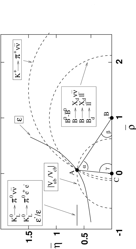
Figure 13: The ideal Unitarity Triangle. For artistic reasons the value of $\bar{\eta}$ has been chosen to be higher than the fitted central value $\bar{\eta}\approx 0.4.$

3.6 CKM Matrix from Tree Level Decays and Unitarity

In this review we are mainly dealing with the physics of heavy flavours. Therefore we will comment only briefly on the determination of the CKM elements describing the mixing between light quarks. The interested reader should simply have a look at the 1996 report of the Particle Data Group [60] where the subject is reviewed and further references can be found. The numbers quoted for the Cabibbo sector of the mixing matrix are taken from there. The remaining entries are sometimes different in view of the most recent developments. We will also be very brief on the determination of $|V_{ub}|$ and $|V_{cb}|$ from $B$ decays as this subject is discussed by Neubert in another chapter of this book. Concerning the top quark couplings $|V_{td}|$, $|V_{ts}|$ and $|V_{tb}|$ we will give here only the ranges following from tree level decays and the unitarity of the CKM matrix. The determination of $|V_{td}|$, $|V_{ts}|$ and of the parameters $\varrho$ and $\eta$ from FCNC processes will, however, be an important topic of the subsequent sections.

3.6.1 Determination of $|V_{ud}|$

$|V_{ud}|$ is mainly determined by comparing superallowed beta decays, i.e. those with pure vector transitions, to muon decay. The measurements are very accurate and therefore the theoretical treatment requires a very careful consideration of radiative corrections. The final result quoted in [60] reads:

$$|V_{ud}|=0.9736\pm 0.0010\,.$$ (3.48)

A more accurate and slightly higher value

$$|V_{ud}|=0.9740\pm 0.0005$$ (3.49)

has been obtained subsequently in a recent experiment on $0^{+}\to 0^{+}$ superallowed beta decays at Chalk River Laboratory [67].

3.6.2 Determination of $|V_{us}|$

There are mainly two ways to determine $|V_{us}|$: via $K_{e3}$ decays and via semileptonic hyperon decays. We will first deal with $K_{e3}$ decays, $K^{+}\to\pi^{0}e^{+}\nu_{e}$ and $K_{\rm L}^{0}\to\pi^{-}e^{+}\nu_{e}$. Being pseudovector $\to$ pseudovector transitions, these decays proceed via pure vector currents and therefore involve $SU(3)$ symmetry breaking in second order only. The corrections have been calculated in chiral perturbation theory [68] yielding $|V_{us}|=0.2196\pm 0.0023$.

Semileptonic hyperon decays are governed not only by vector but also by axialvector currents. The latter break $SU(3)$ already in first order which introduces considerably higher theoretical uncertainties in the extraction of $|V_{us}|$ from experimental data than in $K_{e3}$ decays. However, a careful calculation of $SU(3)$ symmetry breaking effects [69] allows to extract $|V_{us}|$ with reasonable accuracy from these decays. One finds [60] $|V_{us}|=0.222\pm 0.003$.

Combining these two determinations leads to the well known result

$$|V_{us}|=\lambda=0.2205\pm 0.0018\,.$$ (3.50)

In view of the very small error ($1\%$) we will set $\lambda=0.22$ in all numerical calculations.

From (3.48), (3.50) and $|V_{ub}|$ given in (3.57) one finds

$$|V_{ud}|^{2}+|V_{us}|^{2}+|V_{ub}|^{2}=0.9965\pm 0.0021\,,$$ (3.51)

where the contribution of $|V_{ub}|^{2}$ is negligible. Using (3.49) one finds [67]

$$|V_{ud}|^{2}+|V_{us}|^{2}+|V_{ub}|^{2}=0.9972\pm 0.0013.$$ (3.52)

Thus the departure from the unitarity relation (3.23) is by at least two standard deviations. The simplest solution to this “unitarity problem” would be to double the error in $|V_{ud}|$ or to increase its value. Since the neutron decay data give, on the other hand, values for the unitarity sum higher than unity [67], such a shift is certainly possible. Clearly the current status of the $|V_{ud}|$ determinations, in spite of small errors quoted above, is unsatisfactory at present. Further efforts should be made before one could conclude that the failure to meet the unitarity constraint signals some physics beyond the Standard Model.

3.6.3 Determination of $|V_{cd}|$

$|V_{cd}|$ is deduced from single charm production in deep inelastic neutrino (antineutrino) – nucleon scattering supplemented by measurements of semileptonic branching fractions of charmed mesons. The older value based mainly on CDHS data ($|V_{cd}|=0.204\pm 0.017$) has been shifted upwards by the most recent Tevatron data [70] so that the final value quoted in [60] reads

$$|V_{cd}|=0.224\pm 0.016.$$ (3.53)

3.6.4 Determination of $|V_{cs}|$

Here data from deep–inelastic scattering cannot be used as efficiently as in the case of $|V_{cd}|$ since one cannot eliminate all unknown quantities but has to deal with the fairly unknown strange–quark distribution. With conservative assumptions only a very weak lower bound $|V_{cs}|>0.59$ can be obtained. Therefore one tries to determine $|V_{cs}|$ from $D_{e3}$ decays, analogously to $|V_{us}|$, by comparing the data with the theoretical decay width. This implies the use of model dependent formfactors which introduce a considerable uncertainty in the final result [60]:

$$|V_{cs}|=1.01\pm 0.18.$$ (3.54)

Especially in this case unitarity helps a lot to constrain the allowed range as will be seen later.

3.6.5 Determination of $|V_{cb}|$

Clearly during the last two years there has been a considerable progress done by experimentalists and theorists in the extraction of $|V_{cb}|$ from exclusive and inclusive decays. In particular we would like to mention important papers by Shifman, Uraltsev and Vainshtein [72], Neubert [73] and Ball, Benecke and Braun [32] on the basis of which one is entitled to use the value

$$|V_{cb}|=0.040\pm 0.003$$ (3.55)

which should be compared with $|V_{cb}|=0.041\pm 0.006$ used in the Top Quark Story [3]. The value in (3.55) is compatible with the value of Neubert ($|V_{cb}|=0.039\pm 0.002$) given in this book and the ones given in [74, 71, 60]. More details can be found in the chapter by Neubert.

3.6.6 Determination of $|V_{ub}|$

In the case of $|V_{ub}|$ the situation is much worse but progress in the next few years is to be expected in particular due to new information coming from exclusive decays [75, 71], the inclusive semileptonic $b\to u$ rate [72, 32, 76], and the hadronic energy spectrum in $B\to X_{u}e\bar{\nu}_{e}$ [77]. Combining the experimental and theoretical uncertainties one has [60]

$$\frac{|V_{ub}|}{|V_{cb}|}=0.08\pm 0.02$$ (3.56)

which should be compared with $|V_{ub}/V_{cb}|=0.13\pm 0.04$ used in the Top Quark Story [3]. Together with (3.55) this implies

$$|V_{ub}|=(3.2\pm 0.8)\cdot 10^{-3}.$$ (3.57)

3.6.7 Determination of $|V_{td}|$, $|V_{ts}|$ and $|V_{tb}|$

For completeness we would like to make already here a few remarks on the top quark couplings. A more extensive analysis of the couplings $|V_{td}|$ and $|V_{ts}|$ will be performed in subsequent sections.

Setting $\lambda=0.22$, scanning $|V_{cb}|$ and $|V_{ub}/V_{cb}|$ in the ranges (3.55) and (3.56), respectively and $\cos\delta$ in the range $-1\leq\cos\delta\leq 1$, we find the ranges

$$4.5\cdot 10^{-3}\leq|V_{td}|\leq 13.7\cdot 10^{-3}\,,\qquad 0.0353\leq|V_{ts}|\leq 0.0429$$ (3.58)

and

$$0.9991\leq|V_{tb}|\leq 0.9993.$$ (3.59)

The last result should be compared with the direct measurement in top quark decays at Tevatron yielding: $|V_{tb}|>0.58$ at $95\%$ C.L. [92]. From (3.58) we observe that the unitarity of the CKM matrix requires approximate equality of $|V_{ts}|$ and $|V_{cb}|$:

$$0.954\leq\frac{|V_{ts}|}{|V_{cb}|}\leq 0.997$$ (3.60)

which is evident if one compares (3.13) with (3.15). The determination of $|V_{td}|$ will be considerably improved in the next section by using the constraints from $B^{0}_{d}-\bar{B}^{0}_{d}$-mixing and CP violation in the $K$-meson system.

4 $\varepsilon_{K}$, $B^{0}$-$\bar{B}^{0}$ Mixing and the Unitarity Triangle

4.1 Preliminaries

Particle–antiparticle mixing has always been of fundamental importance in testing the Standard Model and often has proven to be an undefeatable challenge for suggested extensions of this model. Particle–antiparticle mixing is responsible for the small mass differences between the mass eigenstates of neutral mesons. Being an FCNC process it involves heavy quarks in loops and consequently it is a perfect testing ground for heavy flavour physics: from the calculation of the $K_{\rm L}-K_{\rm S}$ mass difference, Gaillard and Lee [78] were able to estimate the value of the charm quark mass before charm discovery; $B_{d}^{0}-\bar{B}_{d}^{0}$ mixing [79] gave the first indication of a large top quark mass. Particle–antiparticle mixing is also closely related to the violation of the CP symmetry which is experimentally known since 1964 [80].

In this section we will deal almost exclusively with the parameter $\varepsilon_{K}$ describing so called indirect CP violation in the $K$ system and with the mass differences $\Delta M_{d,s}$ which describe the size of $B_{d,s}^{0}-\bar{B}^{0}_{d,s}$ mixings. In the Standard Model all these phenomena appear first at the one–loop level and as such they are sensitive measures of the top quark couplings $V_{ti}(i=d,s,b)$ and of the top quark mass.

We have seen in section 3 that tree level decays and the unitarity of the CKM matrix give us already a good information about $V_{tb}$ and $V_{ts}$: $V_{tb}\approx 1$ and $\mid V_{ts}\mid\;\approx\;\mid V_{cb}\mid$. Similarly the value of the top quark mass measured by CDF and D0 (see below) is known within $\pm 4\%$. Consequently the main new information to be gained from the quantities discussed here are the values of $|V_{td}|$ and of the phase $\delta$ in the CKM matrix. This will allow us to construct the unitarity triangle.

Let us briefly recall the formalism of particle–antiparticle mixing. We will here mainly discuss the $K$–system as this mixing in the $B$–system is discussed in great detail in section 8. Some formulae for $B_{d,s}^{0}-\bar{B}^{0}_{d,s}$ mixings, necessary for the analysis of the unitarity triangle, are collected in subsection 4.3.

$K^{0}$ and $\bar{K}^{0}$ are flavour eigenstates which in the Standard Model may mix via weak interactions through the box diagrams of fig. 11e. Constructing CP eigenstates and choosing the CKM phase convention $(CP|K^{0}\rangle=|\bar{K}^{0}\rangle)$, we obtain

$$K_{1}={1\over{\sqrt{2}}}(K^{0}+\bar{K}^{0}),\qquad\qquad CP|K_{1}\rangle=|K_{1}\rangle$$ (4.1)

$$K_{2}={1\over{\sqrt{2}}}(K^{0}-\bar{K}^{0}),\qquad\qquad CP|K_{2}\rangle=-|K_{2}\rangle\,.$$ (4.2)

Due to the complex phase in the CKM matrix $K_{1}$ and $K_{2}$ differ from the physical mass eigenstates $K_{\rm S}$ and $K_{\rm L}$, respectively, by a small admixture of the other CP eigenstate:

$$K_{\rm S}={{K_{1}+\bar{\varepsilon}K_{2}}\over{\sqrt{1+\mid\bar{\varepsilon}\mid^{2}}}},\qquad K_{\rm L}={{K_{2}+\bar{\varepsilon}K_{1}}\over{\sqrt{1+\mid\bar{\varepsilon}\mid^{2}}}}\,.$$ (4.3)

The small parameter $\bar{\varepsilon}$ introduced here depends on the phase convention chosen for $K^{0}$ and $\bar{K}^{0}$. Therefore it may not be taken as a physical measure of CP violation.

Since a two pion final state is CP even while a three pion final state is CP odd, $K_{\rm S}$ and $K_{\rm L}$ preferably decay to $2\pi$ and $3\pi$, respectively via the following CP conserving decay modes:

$$K_{\rm L}\to 3\pi{\rm~{}~{}(via~{}K_{2}),}\qquad K_{\rm S}\to 2\pi{\rm~{}~{}(via~{}K_{1}).}$$ (4.4)

This difference is responsible for the large disparity in their life-times. However, since $K_{\rm L}$ and $K_{\rm S}$ are not CP eigenstates they may decay with small branching fractions as follows:

$$K_{\rm L}\to 2\pi{\rm~{}~{}(via~{}K_{1}),}\qquad K_{\rm S}\to 3\pi{\rm~{}~{}(via~{}K_{2}).}$$ (4.5)

Since these decays proceed not via explicit breaking of the CP symmetry in the decay itself but via the admixture of the CP state with opposite CP parity to the dominant one, they are usually called “indirect CP violating”. The measure for this indirect CP violation is then defined as

$$\varepsilon_{K}={{A(K_{\rm L}\rightarrow(\pi\pi)_{I=0}})\over{A(K_{\rm S}\rightarrow(\pi\pi)_{I=0})}},$$ (4.6)

where $\varepsilon_{K}$ is, contrary to $\bar{\varepsilon}$ introduced above, independent of the phase conventions and is measured to be [60]:

$$\varepsilon_{K}^{exp}=(2.280\pm 0.013)\cdot 10^{-3}\;e^{i{\pi\over 4}}\,.$$ (4.7)

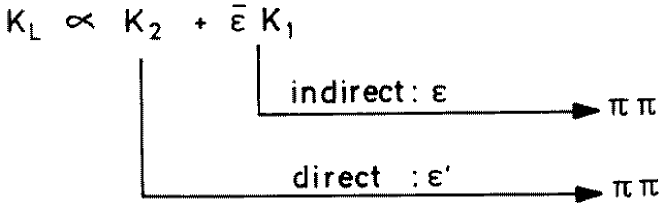
Figure 14: Indirect versus direct CP violation in $K_{L}\to\pi\pi$.

While indirect CP violation reflects the fact that the mass eigenstates are not CP eigenstates, so-called direct CP violation is realized via a direct transition of a CP odd to a CP even state or vice versa (see fig. 14). The parameter $\varepsilon^{\prime}$ is defined as

$$\varepsilon^{\prime}={1\over{\sqrt{2}}}{\rm Im}\left({{A_{2}}\over{A_{0}}}\right)e^{i\Phi}\,,$$ (4.8)

where the isospin amplitudes $A_{I}$ in $K\to\pi\pi$ decays are introduced through

$$A(K^{+}\rightarrow\pi^{+}\pi^{0})=\sqrt{3\over 2}A_{2}e^{i\delta_{2}}$$ (4.9)

$$A(K^{0}\rightarrow\pi^{+}\pi^{-})=\sqrt{2\over 3}A_{0}e^{i\delta_{0}}+\sqrt{1\over 3}A_{2}e^{i\delta_{2}}$$ (4.10)

$$A(K^{0}\rightarrow\pi^{0}\pi^{0})=\sqrt{2\over 3}A_{0}e^{i\delta_{0}}-2\sqrt{1\over 3}A_{2}e^{i\delta_{2}}\,.$$ (4.11)

Here the subscript $I=0,2$ denotes states with isospin $0,2$ equivalent to $\Delta I=1/2$ and $\Delta I=3/2$ transitions, respectively, and $\delta_{0,2}$ are the corresponding strong phases. Finally $\Phi=\pi/2+\delta_{2}-\delta_{0}\approx\pi/4$.

Experimentally $\varepsilon_{K}\equiv\varepsilon$ and $\varepsilon^{\prime}$ can be found by measuring the ratios

$$\eta_{00}={{A(K_{\rm L}\to\pi^{0}\pi^{0})}\over{A(K_{\rm S}\to\pi^{0}\pi^{0})}}\simeq\varepsilon-2\varepsilon^{\prime},~{}~{}~{}~{}\eta_{+-}={{A(K_{\rm L}\to\pi^{+}\pi^{-})}\over{A(K_{\rm S}\to\pi^{+}\pi^{-})}}\simeq\varepsilon+\varepsilon^{\prime},$$ (4.12)

$$\mid{{\eta_{00}}\over{\eta_{+-}}}\mid^{2}\simeq 1-6\;{\rm Re}(\frac{\varepsilon^{\prime}}{\varepsilon})\,.$$ (4.13)

The strength of $K^{0}$–$\bar{K}^{0}$ mixing is described by the $K_{\rm L}-K_{\rm S}$ mass difference which is experimentally measured to be [60]

$$\Delta M_{K}=M(K_{\rm L})-M(K_{\rm S})=(3.491\pm 0.009)\cdot 10^{-15}\,{\rm GeV}\,.$$ (4.14)

In the Standard Model roughly $70\%$ of the measured $\Delta M_{K}$ is described by the real parts of the box diagrams in fig. 11e [43]. The rest is attributed to long distance contributions which are difficult to estimate. For this reason in the theoretical analysis of $\varepsilon_{K}$ it is customary to use the experimental value of $\Delta M_{K}$. On the other hand the parameter $\varepsilon_{K}$ is given (see below) by the imaginary part of the relevant off-diagonal element $M_{12}$ in the neutral $K$-meson mass matrix. The latter being related to CP violation and top quark physics should be dominated by short distance contributions and well approximated by the imaginary parts of the box diagrams in fig. 11e.

Similarly the strength of the $B^{0}_{d,s}-\bar{B}^{0}_{d,s}$ mixings is described by the mass differences

$$\Delta M_{d,s}=M_{H}^{d,s}-M_{L}^{d,s}$$ (4.15)

with “H” and “L” denoting heavy and light respectively. In contrast to $\Delta M_{K}$ , in this case the long distance contributions are estimated to be very small and $\Delta M_{d,s}$ is very well approximated by the relevant box diagrams as discussed below.

After these general remarks we are ready to enter the details.

4.2 Basic Formula for $\varepsilon_{K}$

Indirect CP violation in $K_{\rm L}\to\pi\pi$ is described by the parameter $\varepsilon_{K}$ defined in (4.6). The general formula for $\varepsilon_{K}$ is given as follows:

$$\varepsilon_{K}=\frac{\exp(i\pi/4)}{\sqrt{2}\Delta M_{K}}\,\left({\rm Im}M_{12}+2\xi{\rm Re}M_{12}\right),$$ (4.16)

where

$$\xi=\frac{{\rm Im}A_{0}}{{\rm Re}A_{0}}$$ (4.17)

with $A_{0}\equiv A(K\to(\pi\pi)_{I=0})$ and $\Delta M_{K}$ denoting the $K_{\rm L}$-$K_{\rm S}$ mass difference. The off-diagonal element $M_{12}$ in the neutral $K$-meson mass matrix represents $K^{0}$-$\bar{K}^{0}$ mixing. It is given by

$$2m_{K}M^{*}_{12}=\langle\bar{K}^{0}|{\cal H}_{\rm eff}(\Delta S=2)|K^{0}\rangle\,,$$ (4.18)

where ${\cal H}_{\rm eff}(\Delta S=2)$ is the effective Hamiltonian for the $\Delta S=2$ transitions.

To lowest order these transitions are induced through the box diagrams shown in fig. 11e. Including QCD corrections, the effective low energy Hamiltonian, to be derived from these diagrams, can be written as follows $(\lambda_{i}=V_{is}^{*}V_{id})$ [4]:

$${\cal H}^{\Delta S=2}_{\rm eff} = \frac{G^{2}_{\rm F}}{16\pi^{2}}M^{2}_{W}\left[\lambda^{2}_{c}\eta_{1}S_{0}(x_{c})+\lambda^{2}_{t}\eta_{2}S_{0}(x_{t})+2\lambda_{c}\lambda_{t}\eta_{3}S_{0}(x_{c},x_{t})\right]\times$$ (4.19)

$$\times\left[\alpha_{s}^{(3)}(\mu)\right]^{-2/9}\left[1+\frac{\alpha_{s}^{(3)}(\mu)}{4\pi}J_{3}\right]Q(\Delta S=2)+h.c.$$

This expression is valid for scales $\mu$ below the charm threshold $\mu_{c}={\cal O}(m_{c})$. In this case ${\cal H}^{\Delta S=2}_{\rm eff}$ consists of a single four-quark operator

$$Q(\Delta S=2)=(\bar{s}d)_{V-A}(\bar{s}d)_{V-A},$$ (4.20)

which is multiplied by the corresponding coefficient function. It is useful and customary to decompose this function into a charm-, a top- and a mixed charm-top contribution as displayed in (4.19). This form is obtained upon eliminating $\lambda_{u}$ by means of the unitarity of the CKM matrix and setting $x_{u}=0$. The basic electroweak loop contributions without QCD correction are then expressed through the functions $S_{0}$ calculated in [18] and given in (2.30,2.31).
Short-distance QCD effects are described through the correction factors $\eta_{1}$, $\eta_{2}$, $\eta_{3}$ and the explicitly $\alpha_{s}$-dependent terms in (4.19). The latter terms are factored out to exhibit the $\mu$-dependence of the coefficient function in the $f=3$ regime which has to cancel the corresponding $\mu$-dependence of the hadronic matrix element of $Q$ between meson states in physical applications. A similar comment applies to the renormalization scheme dependence present in $J_{3}$. In the NDR scheme $J_{3}=1.895$. All these issues are discussed in detail in [4].
Without QCD, i.e. in the limit $\alpha_{s}\to 0$, one has $\eta_{i}[\alpha_{s}]^{-2/9}\to 1$. The NLO values of the QCD factors $\eta_{1}$ , $\eta_{2}$ and $\eta_{3}$ are given as follows [43, 44, 45]:

$$\eta_{1}=1.38\pm 0.20,\qquad\eta_{2}=0.57\pm 0.01,\qquad\eta_{3}=0.47\pm 0.04.$$ (4.21)

The quoted errors reflect the remaining theoretical uncertainties due to $\Lambda_{\overline{MS}}$ and the quark masses. The references to the leading order calculations can be found in [4]. The factor $\eta_{1}$ plays only a minor role in the analysis of $\varepsilon_{K}$ but its enhanced value through NLO corrections [43] is essential for the $K_{\rm L}-K_{\rm S}$ mass difference.
Defining the renormalization group invariant parameter $B_{K}$ by

$$B_{K}=B_{K}(\mu)\left[\alpha_{s}^{(3)}(\mu)\right]^{-2/9}\,\left[1+\frac{\alpha_{s}^{(3)}(\mu)}{4\pi}J_{3}\right]$$ (4.22)

$$\langle\bar{K}^{0}|(\bar{s}d)_{V-A}(\bar{s}d)_{V-A}|K^{0}\rangle\equiv\frac{8}{3}B_{K}(\mu)F_{K}^{2}m_{K}^{2}$$ (4.23)

and using (4.19) one finds

$$M_{12}=\frac{G_{\rm F}^{2}}{12\pi^{2}}F_{K}^{2}B_{K}m_{K}M_{\rm W}^{2}\left[{\lambda_{c}^{*}}^{2}\eta_{1}S_{0}(x_{c})+{\lambda_{t}^{*}}^{2}\eta_{2}S_{0}(x_{t})+2{\lambda_{c}^{*}}{\lambda_{t}^{*}}\eta_{3}S_{0}(x_{c},x_{t})\right],$$ (4.24)

where $F_{K}$ is the $K$-meson decay constant and $m_{K}$ the $K$-meson mass.

The last term in (4.16) constitutes at most a 2 % correction to $\varepsilon_{K}$ and consequently can be neglected in view of other uncertainties, in particular those connected with $B_{K}$. Inserting (4.24) into (4.16) one finds

$$\varepsilon_{K}=C_{\varepsilon}B_{K}{\rm Im}\lambda_{t}\left\{{\rm Re}\lambda_{c}\left[\eta_{1}S_{0}(x_{c})-\eta_{3}S_{0}(x_{c},x_{t})\right]-{\rm Re}\lambda_{t}\eta_{2}S_{0}(x_{t})\right\}\exp(i\pi/4)\,,$$ (4.25)

where we have used the unitarity relation ${\rm Im}\lambda_{c}^{*}={\rm Im}\lambda_{t}$ and have neglected ${\rm Re}\lambda_{t}/{\rm Re}\lambda_{c}={\cal O}(\lambda^{4})$ in evaluating ${\rm Im}(\lambda_{c}^{*}\lambda_{t}^{*})$. The numerical constant $C_{\varepsilon}$ is given by

$$C_{\varepsilon}=\frac{G_{\rm F}^{2}F_{K}^{2}m_{K}M_{\rm W}^{2}}{6\sqrt{2}\pi^{2}\Delta M_{K}}=3.78\cdot 10^{4}\,.$$ (4.26)

Using the standard parametrization of (3.5) to evaluate ${\rm Im}\lambda_{i}$ and ${\rm Re}\lambda_{i}$, setting the values for $s_{12}$, $s_{13}$, $s_{23}$ and $m_{\rm t}$ in accordance with section 3 and taking a value for $B_{K}$ (see below), one can determine the phase $\delta$ by comparing (4.25) with the experimental value for $\varepsilon_{K}$.

Once $\delta$ has been determined in this manner one can find the corresponding point $(\bar{\varrho},\bar{\eta})$ by using (3.11) and (3.16). Actually for a given set ($s_{12}$, $s_{13}$, $s_{23}$, $m_{\rm t}$, $B_{K}$) there are two solutions for $\delta$ and consequently two solutions for $(\bar{\varrho},\bar{\eta})$. This will be evident from the analysis of the unitarity triangle presented below.

Concerning the parameter $B_{K}$, the most recent analyses using lattice methods summarized recently by Flynn [81] give $B_{K}=0.90\pm 0.06$. The $1/N$ approach of [82] gives $B_{K}=0.70\pm 0.10$. A recent confirmation of this result in a somewhat modified framework has been presented in [83]. Lower values for $B_{K}$ are obtained by using the QCD Hadronic Duality approach [84] ($B_{K}=0.39\pm 0.10$) or using the $SU(3)$ symmetry and PCAC ($B_{K}=1/3$) [85]. For $|V_{cb}|=0.040$ and $|V_{ub}/V_{cb}|=0.08$ such low values of $B_{K}$ require $m_{\rm t}>200\,{\rm GeV}$ in order to explain the experimental value of $\varepsilon_{K}$ [86, 63, 45]. The QCD sum rule results are in the ball park of $B_{K}=0.60$ [87]. In our numerical analysis presented below we will use

$$B_{K}=0.75\pm 0.15\,.$$ (4.27)

4.3 Basic Formula for $B^{0}$-$\bar{B}^{0}$ Mixing

The strength of $B^{0}$-$\bar{B}^{0}$ mixing is described by

$$\Delta M_{q}=2|M_{12}^{(q)}|,\qquad q=d,s,$$ (4.28)

the mass difference between the mass eigenstates in the $B_{d}^{0}-\bar{B}_{d}^{0}$ system and the $B_{s}^{0}-\bar{B}_{s}^{0}$ system, respectively. Equivalently one can use

$$x_{q}\equiv\frac{\Delta M_{q}}{\Gamma_{B_{q}}},$$ (4.29)

where $\Gamma_{B_{q}}=1/\tau_{B_{q}}$ with $\tau_{B_{q}}$ being the corresponding lifetimes. In what follows we will work dominantly with $\Delta M_{q}$ as this avoids the experimental errors in lifetimes. Moreover this is the way the most recent experimental results for $B^{0}-\bar{B}^{0}$ mixing are quoted.

The off-diagonal term $M_{12}$ in the neutral $B$-meson mass matrix is given by

$$2m_{B_{q}}|M_{12}^{(q)}|=|\langle\bar{B}^{0}_{q}|{\cal H}_{\rm eff}(\Delta B=2)|B^{0}_{q}\rangle|,$$ (4.30)

where ${\cal H}_{\rm eff}(\Delta B=2)$, relevant for scales scales $\mu_{b}={\cal O}(m_{b})$, is the effective Hamiltonian analogous to (4.19) and given in the case of $B_{d}^{0}-\bar{B}_{d}^{0}$ mixing by [44]

$${\cal H}^{\Delta B=2}_{\rm eff}=\frac{G^{2}_{\rm F}}{16\pi^{2}}M^{2}_{W}\left(V^{\ast}_{tb}V_{td}\right)^{2}\eta_{B}S_{0}(x_{t})\left[\alpha^{(5)}_{s}(\mu_{b})\right]^{-6/23}\left[1+\frac{\alpha^{(5)}_{s}(\mu_{b})}{4\pi}J_{5}\right]Q(\Delta B=2)+h.c.$$ (4.31)

Here

$$Q(\Delta B=2)=(\bar{b}d)_{V-A}(\bar{b}d)_{V-A}$$ (4.32)

and $\eta_{B}$ is the QCD factor analogous to $\eta_{2}$ and given by [44]

$$\eta_{B}=0.55\pm 0.01.$$ (4.33)

$J_{5}=1.627$ in the NDR scheme. In the case of $B_{s}^{0}-\bar{B}_{s}^{0}$ mixing one should simply replace $d\to s$ in (4.31) and (4.32) with all other quantities unchanged.

Due to the particular hierarchy of the CKM matrix elements only the top sector can contribute significantly to $B^{0}-\bar{B}^{0}$ mixing. In contrast to the $K^{0}-\bar{K}^{0}$ case, the charm sector and the mixed top-charm contributions are entirely negligible here which considerably simplifies the analysis.

Defining the renormalization group invariant parameters $B_{q}$ by

$$B_{B_{q}}=B_{B_{q}}(\mu)\left[\alpha_{s}^{(5)}(\mu)\right]^{-6/23}\,\left[1+\frac{\alpha_{s}^{(5)}(\mu)}{4\pi}J_{5}\right]$$ (4.34)

$$\langle\bar{B}^{0}_{q}|(\bar{b}q)_{V-A}(\bar{b}q)_{V-A}|B^{0}_{q}\rangle\equiv\frac{8}{3}B_{B_{q}}(\mu)F_{B_{q}}^{2}m_{B_{q}}^{2}\,,$$ (4.35)

where $F_{B_{q}}$ is the $B_{q}$-meson decay constant and using (4.31) one finds

$$\Delta M_{q}=\frac{G_{\rm F}^{2}}{6\pi^{2}}\eta_{B}m_{B_{q}}(B_{B_{q}}F_{B_{q}}^{2})M_{\rm W}^{2}S_{0}(x_{t})|V_{tq}|^{2},$$ (4.36)

which implies

$$\Delta M_{d}=0.50/{\rm ps}\cdot\left[\frac{\sqrt{B_{B_{d}}}F_{B_{d}}}{200\,{\rm MeV}}\right]^{2}\left[\frac{\overline{m}_{\rm t}(m_{\rm t})}{170~{}GeV}\right]^{1.52}\left[\frac{|V_{td}|}{8.8\cdot 10^{-3}}\right]\left[\frac{\eta_{B}}{0.55}\right]$$ (4.37)

and

$$\Delta M_{s}=15.1/{\rm ps}\cdot\left[\frac{\sqrt{B_{B_{s}}}F_{B_{s}}}{240\,{\rm MeV}}\right]^{2}\left[\frac{\overline{m}_{\rm t}(m_{\rm t})}{170~{}GeV}\right]^{1.52}\left[\frac{|V_{ts}|}{0.040}\right]\left[\frac{\eta_{B}}{0.55}\right]\,.$$ (4.38)

There is a vast literature on the lattice calculations of $F_{B_{d}}$ and $B_{B_{d}}$. The most recent world averages given by Flynn [81] are:

$$F_{B_{d}}=(175\pm 25)\,{\rm MeV}\,,\qquad B_{B_{d}}=1.31\pm 0.03\,.$$ (4.39)

This result for $F_{B_{d}}$ is compatible with the results obtained with the help of QCD sum rules [88]. An interesting upper bound $F_{B_{d}}<195\,{\rm MeV}$ using QCD dispersion relations can be found in [89]. In our numerical analysis we will use $F_{B_{d}}\sqrt{B_{B_{d}}}=(200\pm 40)\,{\rm MeV}$. More details can be found in the chapter by Chris Sachrajda. The experimental situation on $\Delta M_{d}$ has been recently summarized by Gibbons [71] and is given in table 4. For $\tau(B_{d})=1.55~{}{\rm ps}$ one has $x_{d}=0.72\pm 0.03$.

4.4 Standard Analysis of the Unitarity Triangle

With all these formulae at hand we are now in a position to discuss the standard analysis of the unitarity triangle. It proceeds essentially in five steps:

Step 1:

From $b\to c$ transition in inclusive and exclusive $B$ meson decays one finds $|V_{cb}|$ and consequently the scale of the unitarity triangle:

$$|V_{cb}|\quad\Longrightarrow\quad\lambda|V_{cb}|=\lambda^{3}A$$ (4.40)

Step 2:

From $b\to u$ transition in inclusive and exclusive $B$ meson decays one finds $|V_{ub}/V_{cb}|$ and consequently the side $CA=R_{b}$ of the UT:

$$|V_{ub}/V_{cb}|\quad\Longrightarrow\quad R_{b}=\sqrt{\bar{\varrho}^{2}+\bar{\eta}^{2}}=4.44\cdot\left|\frac{V_{ub}}{V_{cb}}\right|$$ (4.41)

Step 3:

From the observed indirect CP violation in $K\to\pi\pi$ described experimentally by the parameter $\varepsilon_{K}$ (4.7) and theoretically by the formula (4.25) one derives, using the approximations (3.17-3.19), the constraint

$$\bar{\eta}\left[(1-\bar{\varrho})A^{2}\eta_{2}S_{0}(x_{t})+P_{0}(\varepsilon)\right]A^{2}B_{K}=0.226,$$ (4.42)

where

$$P_{0}(\varepsilon)=\left[\eta_{3}S_{0}(x_{c},x_{t})-\eta_{1}x_{c}\right]\frac{1}{\lambda^{4}},\qquad x_{t}=\frac{m_{\rm t}^{2}}{M_{\rm W}^{2}}.$$ (4.43)

$P_{0}(\varepsilon)=0.31\pm 0.02$ summarizes the contributions of box diagrams with two charm quark exchanges and the mixed charm-top exchanges. $P_{0}(\varepsilon)$ depends very weakly on $m_{t}$ and its range given above corresponds to $155\,{\rm GeV}\leq m_{t}\leq 185\,{\rm GeV}$.

Equation (4.42) specifies a hyperbola in the $(\bar{\varrho},\bar{\eta})$ plane (see fig. 13). This hyperbola intersects the circle found in step 2 in two points which correspond to the two solutions for $\delta$ mentioned earlier. The position of the hyperbola (4.42) in the $(\bar{\varrho},\bar{\eta})$ plane depends on $m_{\rm t}$, $|V_{cb}|=A\lambda^{2}$ and $B_{K}$. With decreasing $m_{\rm t}$, $|V_{cb}|$ and $B_{K}$ the $\varepsilon_{K}$-hyperbola moves away from the origin of the $(\bar{\varrho},\bar{\eta})$ plane. When the hyperbola and the circle (4.41) touch each other lower bounds consistent with $\varepsilon_{K}^{\rm exp}$ for $m_{\rm t}$, $|V_{cb}|$, $|V_{ub}/V_{cb}|$ and $B_{K}$ can be found. The lower bound on $m_{\rm t}$ is discussed in [86]. Corresponding results for $|V_{ub}/V_{cb}|$ and $B_{K}$ can be found in [45, 4]. Approximate analytic expressions for these bounds have been derived in [86, 4]. One has

$$(m_{\rm t})_{\rm min} = M_{\rm W}\left[\frac{1}{2A^{2}}\left(\frac{1}{A^{2}B_{K}R_{b}}-1.4\right)\right]^{0.658}$$ (4.44)

$$\left|\frac{V_{ub}}{V_{cb}}\right|_{\rm min} = \frac{\lambda}{1-\lambda^{2}/2}\,\left[A^{2}B_{K}\left(2x_{t}^{0.76}A^{2}+1.4\right)\right]^{-1}$$ (4.45)

$$(B_{K})_{\rm min} = \left[A^{2}R_{b}\left(2x_{t}^{0.76}A^{2}+1.4\right)\right]^{-1}.$$ (4.46)

We will return to the bound (4.45) below.

Step 4:

From the observed $B^{0}_{d}-\bar{B}^{0}_{d}$ mixing described experimentally by the mass difference $\Delta M_{d}$ or by the mixing parameter $x_{d}=\Delta M_{d}/\Gamma_{B}$ and theoretically by the formula (4.36), the side $BA=R_{t}$ of the unitarity triangle can be determined:

$$R_{t}=\frac{1}{\lambda}\frac{|V_{td}|}{|V_{cb}|}=1.0\cdot\left[\frac{|V_{td}|}{8.8\cdot 10^{-3}}\right]\left[\frac{0.040}{|V_{cb}|}\right]$$ (4.47)

with

$$|V_{td}|=8.8\cdot 10^{-3}\left[\frac{200\,{\rm MeV}}{\sqrt{B_{B_{d}}}F_{B_{d}}}\right]\left[\frac{170~{}GeV}{\overline{m}_{\rm t}(m_{\rm t})}\right]^{0.76}\left[\frac{\Delta M_{d}}{0.50/{\rm ps}}\right]^{0.5}\sqrt{\frac{0.55}{\eta_{B}}}.$$ (4.48)

Step 5:

The measurement of $B^{0}_{s}-\bar{B}^{0}_{s}$ mixing parametrized by $\Delta M_{s}$ together with $\Delta M_{d}$ allows to determine $R_{t}$ in a different way. Using (4.36) and setting $\Delta M^{{\rm max}}_{d}=0.482/\mbox{ps}$ and $|V_{ts}/V_{cb}|^{{\rm max}}=0.993$ (see table 5) one finds a useful formula [6]:

$$(R_{t})_{\rm max}=1.0\cdot\xi\sqrt{\frac{10.2/ps}{\Delta M_{s}}},\qquad\xi=\frac{F_{B_{s}}\sqrt{B_{B_{s}}}}{F_{B_{d}}\sqrt{B_{B_{d}}}},$$ (4.49)

where $\xi=1$ in the $SU(3)$–flavour limit. Note that $m_{\rm t}$ and $|V_{cb}|$ dependences have been eliminated this way and that $\xi$ should in principle contain much smaller theoretical uncertainties than the hadronic matrix elements in $\Delta M_{d}$ and $\Delta M_{s}$ separately.

The most recent values relevant for (4.49) are:

$$\Delta M_{s}>9.2/{\rm ps}\,,\qquad\xi=1.15\pm 0.05\,.$$ (4.50)

The first number is the improved lower bound quoted in [71] based in particular on ALEPH and DELPHI results. The second number comes from quenched lattice calculations summarized by Flynn in [81]. A similar result has been obtained using QCD sum rules [90]. On the other hand another recent quenched lattice calculation [91] not included in (4.50) finds $\xi\approx 1.3$. Moreover one expects that unquenching will increase the value of $\xi$ in (4.50) by roughly 10% so that values as high as $\xi=1.25-1.30$ are certainly possible even from Flynn’s point of view. For such high values of $\xi$ the lower bound on $\Delta M_{s}$ in (4.50) implies $R_{t}\leq 1.37$ which as we will see below is similar to the bound obtained on the basis of the first four steps alone. On the other hand, for $\xi=1.15$ one finds $R_{t}\leq 1.21$ which puts an additional constraint on the unitarity triangle cutting lower values of $\bar{\varrho}$ and higher values of $|V_{td}|$. In view of remaining large uncertainties in $\xi$ we will not use the constraint from $\Delta M_{s}$ below.

4.5 Messages for UT Practitioners

Before presenting the numerical results of a standard analysis we would like to make a few important messages for UT-practitioners.

4.5.1 Message 1

The parameter $m_{t}$, the top quark mass, used in weak decays is not equal to the one measured by CDF and D0 and used in the electroweak precision studies at LEP, SLD or FNAL. In the latter investigations the so-called pole mass is used, whereas in all the NLO calculations listed in table 1 $m_{t}$ refers to the running current top quark mass normalized at $\mu=m_{t}$: $\overline{m}_{\rm t}(m_{\rm t})$. One has

$$\overline{m}_{\rm t}(m_{\rm t})=m_{\rm t}^{{\rm Pole}}\left[1-\frac{4}{3}\frac{\alpha_{s}(m_{t})}{\pi}\right]$$ (4.51)

so that for $m_{\rm t}={\cal O}(170\,{\rm GeV})$, $\bar{m}_{t}(m_{t})$ is typically by $8\,{\rm GeV}$ smaller than $m_{t}^{\rm Pole}$. This difference matters already because the most recent pole mass value from CDF and D0 has a very small error, $(175\pm 6)\,{\rm GeV}$ [92], implying $(167\pm 6)\,{\rm GeV}$ for $\overline{m}_{\rm t}(m_{\rm t})$. In this review we will often denote this mass by $m_{\rm t}$. Note that we do not include $\alpha_{s}^{2}$ corrections in (4.51), which have to be dropped if one works at the NLO level.

4.5.2 Message 2

When using numerical values for $m_{t}$, $B_{K}$, $B_{B}$ and the QCD factors $\eta_{i}$, care must be taken that they are used consistently. This unfortunately is not always the case. As an example let us consider the theoretical expression for $\Delta M_{d}$ which reads

$$\Delta M_{d}=C_{B}F_{B_{d}}^{2}B_{B_{d}}(\mu_{b})\left[\alpha^{(5)}_{s}(\mu_{b})\right]^{-6/23}\left[1+\frac{\alpha^{(5)}_{s}(\mu_{b})}{4\pi}J_{5}\right]\eta_{B}(\mu_{t},\bar{m}_{t}(\mu_{t}))S_{0}(\bar{x}_{t}(\mu_{t}))|V_{td}|^{2}$$ (4.52)

with $C_{B}$ being a numerical constant and all other quantities defined before. Two relevant scales are $\mu_{b}={\cal O}(m_{b})$ and $\mu_{t}={\cal O}(m_{t})$ which according to the rules of the renormalization group game can be chosen for instance in the ranges $2.5~{}\mbox{GeV}\leq\mu_{b}\leq 10~{}\mbox{GeV}$ and $100\,{\rm GeV}\leq\mu_{t}\leq 300\,{\rm GeV}$, respectively. Here $\mu_{b}$ is the scale at which the relevant $\Delta B=2$ operator is normalized and $\mu_{t}$ is the scale at which $m_{\rm t}$ is defined. Clearly $\Delta M_{d}$ cannot depend on $\mu_{b}$ and $\mu_{t}$. Combining the explicit $\alpha_{s}$ factors in (4.52) with $B_{B_{d}}(\mu_{b})$ as in (4.34) and introducing the renormalization group invariant $B_{B_{d}}$ removes $\mu_{b}$ from phenomenological expressions like (4.48). On the other hand, the $\mu_{t}$ dependence cancels between the last two terms as demonstrated explicitly in [44]. To this end the NLO calculation for $\eta_{B}$ is essential. Otherwise $\Delta M_{d}$ shows a sizable $\mu_{t}$ dependence. It turns out that for a choice $\mu_{t}=m_{t}$, $\eta_{B}$ and similarly $\eta_{2}$ in (4.42) are practically independent of $m_{t}$. This is convenient and has been adopted in [44] and in subsequent NLO calculations. Then $\eta_{B}=0.55$ and $\eta_{2}=0.57$ independent of $m_{t}$.

In the past the explicit $\alpha_{s}$ factors in (4.52) have been combined with $\eta_{B}$ to give the corresponding $\mu_{b}$ dependent QCD factor as high as 0.85. This change is compensated by $B_{B}(\mu_{b})<B_{B}$. In view of the fact that most non-perturbative results are given for $B_{B}$ and $B_{K}$, it is important that this older definition is abandoned.

Similar messages apply to $\eta_{i}$ in the case of $\varepsilon_{K}$.

4.5.3 Message 3

It is sometimes stated in the literature that the QCD factors $\eta_{B}$ for $B^{0}_{d}-\bar{B}^{0}_{d}$ and $B^{0}_{s}-\bar{B}^{0}_{s}$ mixings are roughly equal to each other. They are equal. Indeed, $\eta_{B}$ resulting from short distance QCD calculations is independent of whether $B^{0}_{d}-\bar{B}^{0}_{d}$ or $B^{0}_{s}-\bar{B}^{0}_{s}$ is considered. Consequently the ratio $\Delta M_{d}/\Delta M_{s}$ is independent of $m_{t}$ and short distance QCD corrections. The only difference in these two mixings arises through different CKM factors and through different hadronic matrix elements of the relevant $\Delta B=2$ operators which corresponds to $m_{B_{s}}\not=m_{B_{d}}$, $F_{B_{s}}\not=F_{B_{d}}$ and $B_{B_{s}}\not=B_{B_{d}}$. The last two differences are explicitly summarized by $\xi$ in (4.49).

4.6 Numerical Results

4.6.1 Input Parameters

In table 4 we summarize the input parameters which have been used in the standard analysis presented below.

Quantity	Central	Error
$|V_{cb}|$	0.040	$\pm 0.003$
$|V_{ub}/V_{cb}|$	0.080	$\pm 0.020$
$B_{K}$	0.75	$\pm 0.15$
$\sqrt{B_{d}}F_{B_{d}}$	$200\,{\rm MeV}$	$\pm 40\,{\rm MeV}$
$\sqrt{B_{s}}F_{B_{s}}$	$240\,{\rm MeV}$	$\pm 40\,{\rm MeV}$
$m_{\rm t}$	$167\,{\rm GeV}$	$\pm 6\,{\rm GeV}$
$\Delta M_{d}$	$0.464~{}\mbox{ps}^{-1}$	$\pm 0.018~{}\mbox{ps}^{-1}$
$\Lambda_{\overline{\rm MS}}^{(4)}$	$325\,{\rm MeV}$	$\pm 80\,{\rm MeV}$

Table 4: Collection of input parameters.

4.6.2 $\left|V_{ub}/V_{cb}\right|$, $\left|V_{cb}\right|$ and $\varepsilon_{K}$

The values for $\left|V_{ub}/V_{cb}\right|$ and $\left|V_{cb}\right|$ in table 4 are not correlated with each other. On the other hand such a correlation is present in the analysis of the CP violating parameter $\varepsilon_{K}$ which is roughly proportional to the fourth power of $\left|V_{cb}\right|$ and linear in $\left|V_{ub}/V_{cb}\right|$. It follows that not all values in table 4 are simultaneously consistent with the observed value of $\varepsilon_{K}$. This has been emphasized last year by Herrlich and Nierste [45] and in [4]. Explicitly one has using (4.45):

$$\left|\frac{V_{ub}}{V_{cb}}\right|_{\rm min}=\frac{0.225}{B_{K}A^{2}(2x_{t}^{0.76}A^{2}+1.4)}.$$ (4.53)

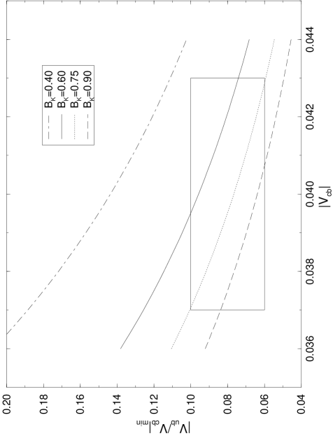
Figure 15: Lower bound on $|V_{ub}/V_{cb}|$ from $\varepsilon_{K}$.

This bound is shown as a function of $|V_{cb}|$ for different values of $B_{K}$ and $m_{\rm t}=173\,{\rm GeV}$ in fig. 15. We observe that simultaneously small values of $\left|V_{ub}/V_{cb}\right|$ and $\left|V_{cb}\right|$, although still consistent with the ones given in table 4, are not allowed by the size of indirect CP violation observed in $K\to\pi\pi$.

4.6.3 Output of a Standard Analysis

The output of the standard analysis depends to some extent on the error analysis. This should always be remembered in view of the fact that different authors use different procedures. In order to illustrate this we show in table 5 the results for various quantities of interest using two types of error analyses:

• Scanning: Both the experimentally measured numbers and the theoretical input parameters are scanned independently within the errors given in table 4.

• Gaussian: The experimentally measured numbers and the theoretical input parameters are used with Gaussian errors.

Clearly the “scanning” method is a bit conservative. On the other hand using Gaussian distributions for theoretical input parameters can certainly be questioned. Personally we think that at present the conservative “scanning” method should be preferred. In the future, however, when data and theory improve, it would be useful to find a less conservative estimate which most probably will give errors somewhere inbetween these two error estimates. The analysis discussed here has been done by Matthias Jamin, Markus Lautenbacher and the first author. More details and more results can be found in [94].

Quantity	Scanning	Gaussian
$\mid V_{td}\mid/10^{-3}$	$6.9-11.3$	$8.6\pm 1.1$
$\mid V_{ts}/V_{cb}\mid$	$0.959-0.993$	$0.976\pm 0.010$
$\mid V_{td}/V_{ts}\mid$	$0.16-0.31$	$0.213\pm 0.034$
$\sin(2\beta)$	$0.36-0.80$	$0.66\pm 0.13$
$\sin(2\alpha)$	$-0.76-1.0$	$0.11\pm 0.55$
$\sin(\gamma)$	$0.66-1.0$	$0.88\pm 0.10$
${\rm Im}\lambda_{t}/10^{-4}$	$0.86-1.71$	$1.29\pm 0.22$
$\Delta M_{s}~{}{\rm ps}$	$8.0-25.4$	$15.2\pm 5.5$

Table 5: Output of the Standard Analysis. $\lambda_{t}=V^{*}_{ts}V_{td}$.

Comparing the results for $|V_{td}|$ with (3.58) we observe that the inclusion of the constraints from $\varepsilon$ and $\Delta M_{d}$ had a considerable impact on the allowed range for this CKM matrix element. Similarly we observe that whereas $\sin 2\beta$ and $\sin\gamma$ are rather constrained, the uncertainty in $\sin 2\alpha$ is huge. Similarly the uncertainties in ${\rm Im}\lambda_{t}$ and $\Delta M_{s}$ are large.

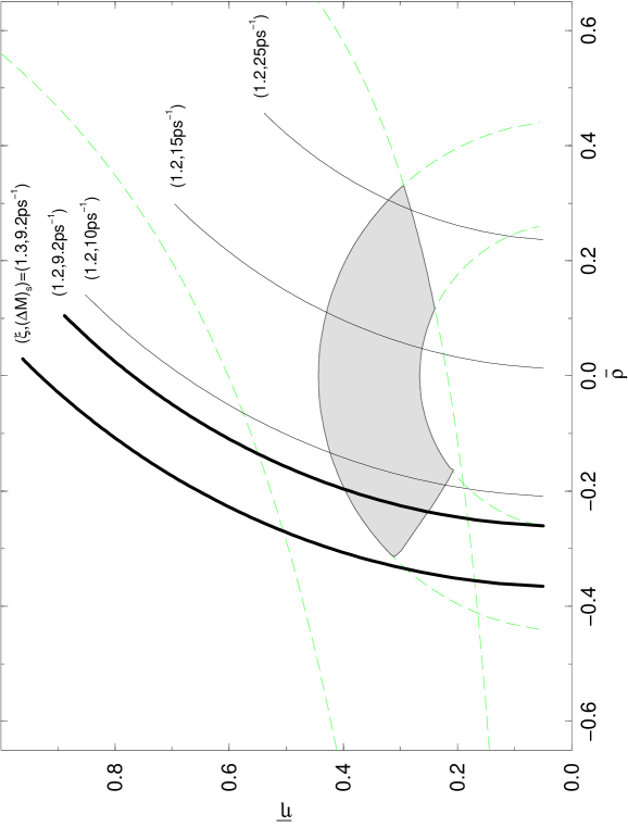
Figure 16: Unitarity Triangle 1997.

In fig. 16 we show the range for the upper corner A of the unitarity triangle. The solid thin lines correspond to $R_{t}^{\rm max}$ from (4.49) using $\xi=1.20$ and $\Delta M_{s}=10/{\rm ps},~{}15/{\rm ps}$ and $25/{\rm ps}$, respectively. The allowed region has a typical “banana” shape which can be found in many other analyses [63, 93, 45, 95, 96, 97]. The size of the banana and its position depends on the assumed input parameters and on the error analysis which varies from paper to paper. The results in fig. 16 correspond to a simple independent scanning of all parameters within one standard deviation. Such an approach is more conservative than using Gaussian distributions as done in some papers quoted above. We show also the impact of the experimental bound $\Delta M_{s}>9.2/{\rm ps}$ with $\xi=1.20$ and the corresponding bound for $\xi=1.30$. In view of the remaining uncertainty in $\xi$, in particular due to quenching in lattice calculations, this bound has not been used in obtaining the results in table 5. It is evident, however, that $B^{0}_{s}-\bar{B}^{0}_{s}$ mixing will have a considerable impact on the unitarity triangle when the value of $\xi$ will be known better and data improves. This is very desirable because as seen in fig. 16 our knowledge of the unitarity triangle is still rather poor.

5 $\varepsilon^{\prime}/\varepsilon$ in the Standard Model

5.1 Preliminaries

Direct CP violation remains one of the important targets of contemporary particle physics. In this respect the search for direct CP violation in $K\to\pi\pi$ decays plays a special role as already fifteen years have been devoted to this enterprise. In this case, a non-vanishing value of the ratio Re($\varepsilon^{\prime}/\varepsilon$) defined in (4.8) would give the first signal for direct CP violation ruling out superweak models. The experimental situation of Re($\varepsilon^{\prime}/\varepsilon$) is, however, unclear at present:

$$Re(\varepsilon^{\prime}/\varepsilon)=\left\{\begin{array}[]{ll}(23\pm 7)\cdot 10^{-4}&\cite[cite]{[\@@bibref{}{barr:93}{}{}]}\\ (7.4\pm 5.9)\cdot 10^{-4}&\cite[cite]{[\@@bibref{}{gibbons:93}{}{}]}.\end{array}\right.$$ (5.1)

While the result of the NA31 collaboration at CERN [98] clearly indicates direct CP violation, the value of E731 at Fermilab [99] is compatible with superweak theories [100] in which $\varepsilon^{\prime}/\varepsilon=0$. Hopefully, in about two years the experimental situation concerning $\varepsilon^{\prime}/\varepsilon$ will be clarified through the improved measurements by the two collaborations at the $10^{-4}$ level and by the KLOE experiment at DA$\Phi$NE.

There is no question about that direct CP violation is present in the Standard Model. Yet accidentally it could turn out that it will be difficult to see it in $K\to\pi\pi$ decays. Indeed in the Standard Model $\varepsilon^{\prime}/\varepsilon$ is governed by QCD penguins and electroweak (EW) penguins. In spite of being suppressed by $\alpha/\alpha_{s}$ relative to QCD penguin contributions, electroweak penguin contributions have to be included because of the additional enhancement factor ${\rm Re}A_{0}/{\rm Re}A_{2}=22$ (see (5.2)-(5.4)) relative to QCD penguins. With increasing $m_{\rm t}$ the EW penguins become increasingly important [101, 102] and, entering $\varepsilon^{\prime}/\varepsilon$ with the opposite sign to QCD penguins, suppress this ratio for large $m_{\rm t}$. For $m_{\rm t}\approx 200\,\,{\rm GeV}$ the ratio can even be zero [102]. Because of this strong cancellation between two dominant contributions and due to uncertainties related to hadronic matrix elements of the relevant local operators, a precise prediction of $\varepsilon^{\prime}/\varepsilon$ is not possible at present. We will discuss this in detail below.

The first calculations of $\varepsilon^{\prime}/\varepsilon$ for $m_{\rm t}\ll M_{\rm W}$ and in the leading order approximation can be found in [103]. For $m_{\rm t}\ll M_{\rm W}$ only $QCD$ penguins play a substantial role. Over the eighties these calculations were refined through the inclusion of isospin braking in the quark masses [104, 105, 106], the inclusion of QED penguin effects for $m_{\rm t}\ll M_{\rm W}$ [107, 104, 105], and through improved estimates of hadronic matrix elements in the framework of the $1/N$ approach [108]. This era of $\varepsilon^{\prime}/\varepsilon$ culminated in the analyses in [101, 102], where QCD penguins, electroweak penguins ($\gamma$ and $Z^{0}$ penguins) and the relevant box diagrams were included for arbitrary top quark masses. The strong cancellation between QCD penguins and electroweak penguins for $m_{t}>150~{}\,{\rm GeV}$ found in these papers was confirmed by other authors [109].

All these calculations were done in the leading logarithmic approximation (e.g. one-loop anomalous dimensions of the relevant operators) with the exception of the $m_{\rm t}$-dependence which in the analyses [101, 102, 109] has been already included at the NLO level. While such a procedure is not fully consistent, it allowed for the first time to exhibit the strong $m_{\rm t}$-dependence of the electroweak penguin contributions, which is not seen in a strict leading logarithmic approximation.

During the nineties considerable progrees has been made by calculating complete NLO corrections to $\varepsilon^{\prime}$ [35, 36, 23, 37, 38]. Together with the NLO corrections to $\varepsilon_{K}$ and $B^{0}-\bar{B}^{0}$ mixing discussed in the previous section, this allows a complete NLO analysis of $\varepsilon^{\prime}/\varepsilon$ including constraints from the observed indirect CP violation ($\varepsilon_{K}$) and $B^{0}-\bar{B}^{0}$ mixing ($\Delta M_{d,s}$). The improved determination of the $V_{ub}$ and $V_{cb}$ elements of the CKM matrix, the improved estimates of hadronic matrix elements using the lattice approach and in particular the determination of the top quark mass $m_{\rm t}$ had of course also an important impact on $\varepsilon^{\prime}/\varepsilon$.

After these general remarks we will now summarize the present status of $\varepsilon^{\prime}/\varepsilon$ in explicit terms.

5.2 Basic Formulae

The direct CP violation in $K\to\pi\pi$ is described by the parameter $\varepsilon^{\prime}$ defined in (4.8). It is is given in terms of the real and imaginary parts of the amplitudes $A_{0}\equiv A(K\to(\pi\pi)_{I=0})$ and $A_{2}\equiv A(K\to(\pi\pi)_{I=2})$ as follows:

$$\varepsilon^{\prime}=-\frac{\omega}{\sqrt{2}}\xi(1-\Omega)\exp(i\Phi)\,,$$ (5.2)

where

$$\xi=\frac{{\rm Im}A_{0}}{{\rm Re}A_{0}}\,,\quad\omega=\frac{{\rm Re}A_{2}}{{\rm Re}A_{0}}\,,\quad\Omega=\frac{1}{\omega}\frac{{\rm Im}A_{2}}{{\rm Im}A_{0}}$$ (5.3)

and $\Phi=\pi/2+\delta_{2}-\delta_{0}\approx\pi/4$. ${\rm Im}A_{0}$ is dominated by QCD penguins and is very weakly dependent on $m_{\rm t}$. ${\rm Im}A_{2}$ increases on the other hand strongly with $m_{\rm t}$ and for large $m_{\rm t}$ is dominated by electroweak penguins. It receives also a sizable contribution from isospin braking $(m_{u}\not=m_{d})$ which conspires with electroweak penguins to cancel substantially the QCD penguin contribution in ${\rm Im}A_{0}$. The factor $1/\omega\approx 22$ in $\Omega$ giving a large enhancement is to a large extend responsible for this cancellation.

When using (5.2) and (5.3) in phenomenological applications one usually takes ${\rm Re}A_{0}$ and $\omega$ from experiment, i.e.

$${\rm Re}A_{0}=3.33\cdot 10^{-7}\,{\rm GeV},\qquad{\rm Re}A_{2}=1.50\cdot 10^{-8}\,{\rm GeV},\qquad\omega=0.045,$$ (5.4)

where the last relation reflects the so-called $\Delta I=1/2$ rule. The main reason for this strategy is the unpleasant fact that until today nobody succeded in fully explaining this rule which to a large extent is believed to originate in the long-distance QCD contributions [110]. On the other hand the imaginary parts of the amplitudes in (5.3) being related to CP violation and the top quark physics should be dominated by short-distance contributions. Therefore ${\rm Im}A_{0}$ and ${\rm Im}A_{2}$ are usually calculated using the effective Hamiltonian for $\Delta S=1$ transitions:

$${\cal H}_{\rm eff}(\Delta S=1)=\frac{G_{\rm F}}{\sqrt{2}}V_{us}^{*}V_{ud}\sum_{i=1}^{10}\left(z_{i}(\mu)+\tau\;y_{i}(\mu)\right)Q_{i}(\mu)$$ (5.5)

with $\tau=-V_{ts}^{*}V_{td}/(V_{us}^{*}V_{ud})$.

The operators $Q_{i}$ are the analogues of the ones given in (2.61)-(2.65). They are given explicitly as follows:

Current–Current :

$$Q_{1}=(\bar{s}_{\alpha}u_{\beta})_{V-A}\;(\bar{u}_{\beta}d_{\alpha})_{V-A}~{}~{}~{}~{}~{}~{}Q_{2}=(\bar{s}u)_{V-A}\;(\bar{u}d)_{V-A}$$ (5.6)

QCD–Penguins :

$$Q_{3}=(\bar{s}d)_{V-A}\sum_{q=u,d,s}(\bar{q}q)_{V-A}~{}~{}~{}~{}~{}~{}Q_{4}=(\bar{s}_{\alpha}d_{\beta})_{V-A}\sum_{q=u,d,s}(\bar{q}_{\beta}q_{\alpha})_{V-A}$$ (5.7)

$$Q_{5}=(\bar{s}d)_{V-A}\sum_{q=u,d,s}(\bar{q}q)_{V+A}~{}~{}~{}~{}~{}Q_{6}=(\bar{s}_{\alpha}d_{\beta})_{V-A}\sum_{q=u,d,s}(\bar{q}_{\beta}q_{\alpha})_{V+A}$$ (5.8)

Electroweak–Penguins :

$$Q_{7}={3\over 2}\;(\bar{s}d)_{V-A}\sum_{q=u,d,s}e_{q}\;(\bar{q}q)_{V+A}~{}~{}~{}~{}~{}Q_{8}={3\over 2}\;(\bar{s}_{\alpha}d_{\beta})_{V-A}\sum_{q=u,d,s}e_{q}(\bar{q}_{\beta}q_{\alpha})_{V+A}$$ (5.9)

$$Q_{9}={3\over 2}\;(\bar{s}d)_{V-A}\sum_{q=u,d,s}e_{q}(\bar{q}q)_{V-A}~{}~{}~{}~{}~{}Q_{10}={3\over 2}\;(\bar{s}_{\alpha}d_{\beta})_{V-A}\sum_{q=u,d,s}e_{q}\;(\bar{q}_{\beta}q_{\alpha})_{V-A}\,.$$ (5.10)

Here, $e_{q}$ denotes the electrical quark charges reflecting the electroweak origin of $Q_{7},\ldots,Q_{10}$.

The Wilson coefficient functions $z_{i}(\mu)$ and $y_{i}(\mu)$ were calculated including the complete next-to-leading order (NLO) corrections in [35, 36, 23, 37, 38]. The details of these calculations can be found there and in the review [4]. Only the coefficients $y_{i}(\mu)$ enter the evaluation of $\varepsilon^{\prime}/\varepsilon$. Examples of their numerical values are given in table 6. Extensive tables for $y_{i}(\mu)$ can be found in [4].

	$\Lambda_{\overline{\rm MS}}^{(4)}=245\,{\rm MeV}$			$\Lambda_{\overline{\rm MS}}^{(4)}=325\,{\rm MeV}$			$\Lambda_{\overline{\rm MS}}^{(4)}=405\,{\rm MeV}$
Scheme	LO	NDR	HV	LO	NDR	HV	LO	NDR	HV
$z_{1}$	-0.550	-0.364	-0.438	-0.625	-0.415	-0.507	-0.702	-0.469	-0.585
$z_{2}$	1.294	1.184	1.230	1.345	1.216	1.276	1.399	1.251	1.331
$y_{3}$	0.029	0.024	0.027	0.034	0.029	0.033	0.039	0.034	0.039
$y_{4}$	-0.054	-0.050	-0.052	-0.061	-0.057	-0.060	-0.068	-0.065	-0.068
$y_{5}$	0.014	0.007	0.014	0.015	0.005	0.016	0.016	0.002	0.018
$y_{6}$	-0.081	-0.073	-0.067	-0.096	-0.089	-0.081	-0.113	-0.109	-0.097
$y_{7}/\alpha$	0.032	-0.031	-0.030	0.039	-0.030	-0.028	0.045	-0.029	-0.026
$y_{8}/\alpha$	0.100	0.111	0.120	0.121	0.136	0.145	0.145	0.166	0.176
$y_{9}/\alpha$	-1.445	-1.437	-1.437	-1.490	-1.479	-1.479	-1.539	-1.528	-1.528
$y_{10}/\alpha$	0.588	0.477	0.482	0.668	0.547	0.553	0.749	0.624	0.632

Table 6: $\Delta S=1$ Wilson coefficients at $\mu=m_{\rm c}=1.3\,{\rm GeV}$ for $m_{\rm t}=170\,{\rm GeV}$ and $f=3$ effective flavours. $|z_{3}|,\ldots,|z_{10}|$ are numerically irrelevant relative to $|z_{1,2}|$. $y_{1}=y_{2}\equiv 0$.

Using the Hamiltonian in (5.5) and the experimental values for $\varepsilon$, ${\rm Re}A_{0}$ and $\omega$ the ratio $\varepsilon^{\prime}/\varepsilon$ can be written as follows:

$$\frac{\varepsilon^{\prime}}{\varepsilon}={\rm Im}\lambda_{t}\cdot\left[P^{(1/2)}-P^{(3/2)}\right],$$ (5.11)

where

$$P^{(1/2)} = r\sum y_{i}\langle Q_{i}\rangle_{0}(1-\Omega_{\eta+\eta^{\prime}})$$ (5.12)

$$P^{(3/2)} = \frac{r}{\omega}\sum y_{i}\langle Q_{i}\rangle_{2}~{}~{}~{}~{}~{}~{}$$ (5.13)

with

$$r=\frac{G_{\rm F}\omega}{2|\varepsilon|{\rm Re}A_{0}}\,\qquad\langle Q_{i}\rangle_{I}\equiv\langle(\pi\pi)_{I}|Q_{i}|K\rangle.$$ (5.14)

Note that the overall phases in $\varepsilon^{\prime}$ and $\varepsilon$ cancel in the ratio to an excellent approximation. The sum in (5.12) and (5.13) runs over all contributing operators. $P^{(3/2)}$ is fully dominated by electroweak penguin contributions. $P^{(1/2)}$ on the other hand is governed by QCD penguin contributions which are suppressed by isospin breaking in the quark masses ($m_{u}\not=m_{d}$). The latter effect is described by

$$\Omega_{\eta+\eta^{\prime}}=\frac{1}{\omega}\frac{({\rm Im}A_{2})_{\rm I.B.}}{{\rm Im}A_{0}}\,.$$ (5.15)

For $\Omega_{\eta+\eta^{\prime}}$ we will take

$$\Omega_{\eta+\eta^{\prime}}=0.25\pm 0.05\,,$$ (5.16)

which is in the ball park of the values obtained in the $1/N_{c}$ approach [105] and in chiral perturbation theory [104, 106]. $\Omega_{\eta+\eta^{\prime}}$ is independent of $m_{\rm t}$.

The main source of uncertainty in the calculation of $\varepsilon^{\prime}/\varepsilon$ are the hadronic matrix elements $\langle Q_{i}\rangle_{I}$. They depend generally on the renormalization scale $\mu$ and on the scheme used to renormalize the operators $Q_{i}$. These two dependences are canceled by those present in the Wilson coefficients $y_{i}(\mu)$ so that the resulting physical $\varepsilon^{\prime}/\varepsilon$ does not (in principle) depend on $\mu$ and on the renormalization scheme of the operators. Unfortunately the accuracy of the present non-perturbative methods used to evalutate $\langle Q_{i}\rangle_{I}$, like lattice methods or the $1/N_{c}$ expansion, is not sufficient to obtain the required $\mu$ and scheme dependences of $\langle Q_{i}\rangle_{I}$. A review of the existing methods and their comparison can be found in [23], [93].

In view of this situation it has been suggested in [23] to determine as many matrix elements $\langle Q_{i}\rangle_{I}$ as possible from the leading CP conserving $K\to\pi\pi$ decays, for which the experimental data are summarized in (5.4). To this end it turned out to be very convenient to determine $\langle Q_{i}\rangle_{I}$ at a scale $\mu=m_{\rm c}$. Using the renormalization group evolution one can then find $\langle Q_{i}\rangle_{I}$ at any other scale $\mu\not=m_{\rm c}$. The details of this procedure can be found in [23]. We will briefly summarize the most important results of this work below.

5.3 Hadronic Matrix Elements

It is customary to express the matrix elements $\langle Q_{i}\rangle_{I}$ in terms of non-perturbative parameters $B_{i}^{(1/2)}$ and $B_{i}^{(3/2)}$ as follows:

$$\langle Q_{i}\rangle_{0}\equiv B_{i}^{(1/2)}\,\langle Q_{i}\rangle_{0}^{\rm(vac)}\,,\qquad\langle Q_{i}\rangle_{2}\equiv B_{i}^{(3/2)}\,\langle Q_{i}\rangle_{2}^{\rm(vac)}\,.$$ (5.17)

The label “vac” stands for the vacuum insertion estimate of the hadronic matrix elements in question. It suffices to give here only a few examples [23]:

$$\langle Q_{1}\rangle_{0} = -\,\frac{1}{9}XB_{1}^{(1/2)}\,,$$ (5.18)

$$\langle Q_{2}\rangle_{0} = \frac{5}{9}XB_{2}^{(1/2)}\,,$$ (5.19)

$$\langle Q_{6}\rangle_{0} = -\,4\sqrt{\frac{3}{2}}\left[\frac{m_{\rm K}^{2}}{m_{\rm s}(\mu)+m_{\rm d}(\mu)}\right]^{2}\frac{F_{\pi}}{\kappa}\,B_{6}^{(1/2)}\,,$$ (5.20)

$$\langle Q_{1}\rangle_{2} = \langle Q_{2}\rangle_{2}=\frac{4\sqrt{2}}{9}XB_{1}^{(3/2)}\,,$$ (5.21)

$$\langle Q_{i}\rangle_{2} = 0\,,\qquad i=3,\ldots,6\,,$$ (5.22)

$$\langle Q_{8}\rangle_{2} = -\left[\frac{\kappa}{2\sqrt{2}}\langle\overline{Q_{6}}\rangle_{0}+\frac{\sqrt{2}}{6}X\right]B_{8}^{(3/2)}\,,$$ (5.23)

$$\langle Q_{9}\rangle_{2} = \langle Q_{10}\rangle_{2}=\frac{3}{2}\langle Q_{1}\rangle_{2}\,,$$ (5.24)

where

$$\kappa=\frac{F_{\pi}}{F_{\rm K}-F_{\pi}}\,,\qquad X=\sqrt{\frac{3}{2}}F_{\pi}\left(m_{\rm K}^{2}-m_{\pi}^{2}\right)\,,$$ (5.25)

and

$$\langle\overline{Q_{6}}\rangle_{0}=\frac{\langle Q_{6}\rangle_{0}}{B_{6}^{(1/2)}}\,.$$ (5.26)

In the vacuum insertion method $B_{i}=1$ independent of $\mu$. In QCD, however, the hadronic parameters $B_{i}$ generally depend on the renormalization scale $\mu$ and the renormalization scheme considered.

In view of the smallness of $\tau={\cal O}(10^{-4})$ entering (5.5), the real amplitudes in (5.4) are governed by the coefficients $z_{i}(\mu)$. The method of extracting some of the matrix elements from the data as proposed in [23] relies then on the fact that due to the GIM mechanism the coefficients $z_{i}(\mu)$ of the penguin operators (i=3….10) vanish for $\mu=m_{c}$ in the HV scheme and are negligible in the NDR scheme. This allows to to find

$$\langle Q_{1}(m_{c})\rangle_{2}=\langle Q_{2}(m_{c})\rangle_{2}=\frac{10^{6}\,{\rm GeV}^{2}}{1.77}\frac{{\rm Re}A_{2}}{z_{+}(m_{c})}=\frac{8.47\cdot 10^{-3}\,{\rm GeV}^{3}}{z_{+}(m_{c})}$$ (5.27)

with $z_{+}=z_{1}+z_{2}$ and

$$\langle Q_{1}(m_{\rm c})\rangle_{0}=\frac{10^{6}\,{\rm GeV}^{2}}{1.77}\frac{{\rm Re}A_{0}}{z_{1}(m_{\rm c})}-\frac{z_{2}(m_{\rm c})}{z_{1}(m_{\rm c})}\langle Q_{2}(m_{\rm c})\rangle_{0}\,.$$ (5.28)

Comparing (5.27) with (5.21) one finds immediately

$$B_{1}^{(3/2)}(m_{c})=\frac{0.363}{z_{+}(m_{c})}\,,$$ (5.29)

which using table 6 gives for $m_{\rm c}=1.3\,{\rm GeV}$ and $\Lambda_{\overline{\rm MS}}^{(4)}=325\,{\rm MeV}$

$$B_{1,NDR}^{(3/2)}(m_{\rm c})=0.453\,,\qquad B_{1,HV}^{(3/2)}(m_{\rm c})=0.472\,.$$ (5.30)

The extracted values for $B_{1}^{(3/2)}$ are by more than a factor of two smaller than the vacuum insertion estimate. They are compatible with the $1/N_{c}$ value $B_{1}^{(3/2)}(1\,{\rm GeV})\approx 0.55$ [108] and are somewhat smaller than the lattice result $B_{1}^{(3/2)}(2\,{\rm GeV})\approx 0.6$ [93]. As analyzed in [23], $B_{1}^{(3/2)}(\mu)$ decreases slowly with increasing $\mu$. As seen in (5.24), this analysis gives also $\langle Q_{9}(m_{\rm c})\rangle_{2}$ and $\langle Q_{10}(m_{\rm c})\rangle_{2}$.

In order to extract $B_{1}^{(1/2)}(m_{\rm c})$ and $B_{2}^{(1/2)}(m_{\rm c})$ from (5.28) one can make the very plausible assumption $\langle Q_{-}(m_{\rm c})\rangle_{0}\geq\langle Q_{+}(m_{\rm c})\rangle_{0}\geq 0$, where $Q_{\pm}=(Q_{2}\pm Q_{1})/2$ which is valid in known non-perturbative approaches. This gives for $\Lambda_{\overline{\rm MS}}^{(4)}=325\,{\rm MeV}$

$$B_{2,NDR}^{(1/2)}(m_{\rm c})=6.6\pm 1.0,\qquad B_{2,HV}^{(1/2)}(m_{\rm c})=6.2\pm 1.0\,.$$ (5.31)

The extraction of $B_{1}^{(1/2)}(m_{\rm c})$ and of analogous parameters $B_{3,4}^{(1/2)}(m_{\rm c})$ are presented in detail in [23]. $B_{1}^{(1/2)}(m_{\rm c})$ depends very sensitively on $B_{2}^{(1/2)}(m_{\rm c})$ and its central value is as high as 15. $B_{4}^{(1/2)}(m_{\rm c})$ is typically by (10–15) % lower than $B_{2}^{(1/2)}(m_{\rm c})$. In any case this analysis shows very large deviations from the results of the vacuum insertion method.

The matrix elements of the $(V-A)\otimes(V+A)$ operators $Q_{5}$–$Q_{8}$ cannot be constrained by CP conserving data and one has to rely on existing non-perturbative methods to calculate them. This is rather unfortunate because the QCD penguin operator $Q_{6}$ and the electroweak penguin operator $Q_{8}$, having large Wilson coefficients and large hadronic matrix elements, play the dominant role in $\varepsilon^{\prime}/\varepsilon$.

The values of $B_{i}$ factors describing the matrix elements of $Q_{5}-Q_{8}$ operators are equal to unity in the vacuum insertion method. The same result is found in the large $N$ limit [108, 105]. Also lattice calculations give similar results: $B^{1/2}_{5,6}=1.0\pm 0.2$ [122, 123] and $B^{3/2}_{7,8}=1.0\pm 0.2$ [122]-[125], $B^{3/2}_{8}=0.81(1)$ [117]. These are the values used in [23, 93, 4, 111]. In the chiral quark model one finds [114]: $B^{1/2}_{6}=1.0\pm 0.4$, $B^{3/2}_{8}=2.2\pm 1.5$ and generally $B^{3/2}_{8}>B^{1/2}_{6}$. On the other hand the Dortmund group [113, 115] advocates $B^{1/2}_{6}>B^{3/2}_{8}$. From [115] $B^{1/2}_{6}=1.3$ and $B^{3/2}_{8}=0.7$ can be extracted. Concerning $B_{7,8}^{(1/2)}$ one can simply set $B_{7,8}^{(1/2)}=1$ as the matrix elementes $\langle Q_{7,8}\rangle_{0}$ play only a minor role in the $\varepsilon^{\prime}/\varepsilon$ analysis.

As demonstrated in [23], the parametrs $B_{5,6}^{(1/2)}$ and $B_{7,8}^{(3/2)}$ depend only very weakly on the renormalization scale $\mu$ when $\mu>1\,{\rm GeV}$ is considered. The $\mu$ dependence of the matrix elements $\langle Q_{5,6}\rangle_{0}$ and $\langle Q_{7,8}\rangle_{2}$ is then given to excellent acurracy by the $\mu$ dependence of $m_{\rm s}(\mu)$. For $\langle Q_{6}\rangle_{0}$ and $\langle Q_{8}\rangle_{2}$ this property has been first found in the $1/N_{c}$ approach [105]: in the large-$N_{c}$ limit the anomalous dimensions of $Q_{6}$ and $Q_{8}$ are simply twice the anomalous dimension of the mass operator leading to $\sim 1/m_{\rm s}^{2}(\mu)$ for the corresponding matrix elements. In the numerical renormalization study in [23] the factors $B_{5,6}^{(1/2)}$ and $B_{7,8}^{(3/2)}$ have been set to unity at $\mu=m_{\rm c}$. Subsequently the evolution of the matrix elements in the range $1\,{\rm GeV}\leq\mu\leq 4\,{\rm GeV}$ has been calculated showing that for the NDR scheme $B_{5,6}^{(1/2)}$ and $B_{7,8}^{(3/2)}$ were $\mu$ independent within an accuracy of (2–3) %. The $\mu$ dependence in the HV scheme has been found to be stronger but still below 10 %.

In summary the treatment of $\langle Q_{i}\rangle_{0,2}$, $i=5,\ldots 8$ in [23, 4, 111] is to set

$$B_{7,8}^{(1/2)}(m_{\rm c})=1,\qquad B_{5}^{(1/2)}(m_{\rm c})=B_{6}^{(1/2)}(m_{\rm c}),\qquad B_{7}^{(3/2)}(m_{\rm c})=B_{8}^{(3/2)}(m_{\rm c})$$ (5.32)

and to treat $B_{6}^{(1/2)}(m_{\rm c})$ and $B_{8}^{(3/2)}(m_{\rm c})$ as free parameters in the range

$$B_{6}^{(1/2)}(m_{\rm c})=1.0\pm 0.2,\qquad B_{8}^{(3/2)}(m_{\rm c})=1.0\pm 0.2$$ (5.33)

suggested by lattice calculations. Then the main uncertainty in the values of $\langle Q_{i}\rangle_{0,2}$, $i=5,\ldots 8$ results from the value of the strange quark mass $m_{\rm s}(m_{\rm c})$.

It seems therefore appropriate to summarize now the present status of the value of the strange quark mass. The most recent results of QCD sum rule (QCDSR) calculations [119, 120, 121] obtained at $\mu=1$ GeV correspond to $m_{\rm s}(m_{\rm c})=(170\pm 20)\,\,{\rm MeV}$ with $m_{\rm c}=1.3\,\,{\rm GeV}$. The lattice calculation of [116] finds $m_{\rm s}(2\,\,{\rm GeV})=(128\pm 18)\,\,{\rm MeV}$ which corresponds to $m_{\rm s}(m_{\rm c})=(150\pm 20)\,\,{\rm MeV}$, in rather good agreement with the QCDSR result. In summer 1996 a new lattice result has been presented by Gupta and Bhattacharya [117]. In the quenched approximation they find $m_{\rm s}(2\,\,{\rm GeV})=(90\pm 20)\,\,{\rm MeV}$ corresponding to $m_{\rm s}(m_{\rm c})=(105\pm 20)\,\,{\rm MeV}$. For $n_{f}=2$ the value is found to be even lower: $m_{\rm s}(2\,\,{\rm GeV})=(70\pm 15)\,\,{\rm MeV}$ corresponding to $m_{\rm s}(m_{\rm c})=(82\pm 17)\,\,{\rm MeV}$. Similar results are found by the lattice group at FNAL [118].

The situation with the strange quark mass is therefore unclear at present and it is useful to present the results for its low and high values. Such an analysis has been done recently in [111] in which the values

$$m_{\rm s}(m_{\rm c})=(150\pm 20)\,\,{\rm MeV}\quad{\rm and}\quad m_{\rm s}(m_{\rm c})=(100\pm 20)\,\,{\rm MeV}$$ (5.34)

have been used. The results presented below are the results of this paper. For convenience we also provide in table 7 the dictionary between the values of $m_{\rm s}$ normalized at different scales [111]. To this end the standard renormalization group formula at the two-loop level with $\Lambda_{\overline{\rm MS}}^{(4)}=325~{}\,{\rm MeV}$ has been used.

$m_{\rm s}(m_{\rm c})$	$~{}75$	$100$	$125$	$150$	$175$
$m_{\rm s}(2~{}\,{\rm GeV})$	$~{}64$	$~{}86$	$107$	$129$	$150$
$m_{\rm s}(1~{}\,{\rm GeV})$	$~{}86$	$115$	$144$	$173$	$202$

Table 7: The dictionary between the values of $m_{\rm s}$ in units of $\,{\rm MeV}$ normalized at different scales with $m_{\rm c}=1.3~{}\,{\rm GeV}$.

Finally one should remark that the decomposition of the relevant hadronic matrix elements of penguin operators into a product of $B_{i}$ factors times $1/m_{s}^{2}$, although useful in the $1/N_{c}$ approach, is in principle unnecessary in a brute force method like the lattice approach. It is to be expected that the future lattice calculations will directly give the relevant hadronic matrix elements and the issue of $m_{\rm s}$ in connection with $\varepsilon^{\prime}/\varepsilon$ will effectively disappear.

5.4 An Analytic Formula for $\varepsilon^{\prime}/\varepsilon$

As shown in [126], it is possible to cast the formal expression for $\varepsilon^{\prime}/\varepsilon$ in (5.11) into an analytic formula which exhibits the $m_{\rm t}$ dependence together with the dependence on $m_{\rm s}$, $\Lambda_{\overline{\rm MS}}^{(4)}$, $B_{6}^{(1/2)}$ and $B_{8}^{(3/2)}$. Such an analytic formula should be useful for those phenomenologists and experimentalists who are not interested in getting involved with the technicalities discussed above.

In order to find an analytic expression for $\varepsilon^{\prime}/\varepsilon$, which exactly reproduces the numerical results based on the formal OPE method, one uses the PBE presented in section 2.7. The updated analytic formula for $\varepsilon^{\prime}/\varepsilon$ of [126] presented recently in [111] is given as follows:

$$\frac{\varepsilon^{\prime}}{\varepsilon}={\rm Im}\lambda_{t}\cdot F(x_{t})\,,$$ (5.35)

where

$$F(x_{t})=P_{0}+P_{X}\,X_{0}(x_{t})+P_{Y}\,Y_{0}(x_{t})+P_{Z}\,Z_{0}(x_{t})+P_{E}\,E_{0}(x_{t})$$ (5.36)

and

$${\rm Im}\lambda_{t}={\rm Im}V_{ts}^{*}V_{td}=|V_{\rm ub}|\,|V_{\rm cb}|\,\sin\delta=\eta\,\lambda^{5}\,A^{2}$$ (5.37)

in the standard parameterization of the CKM matrix (3.5) and in the Wolfenstein parameterization (3.8), respectively.

The $m_{\rm t}$-dependent functions in (5.36) are given in (2.27), (2.77), (2.78) and (2.79). The coefficients $P_{i}$ are given in terms of $B_{6}^{(1/2)}\equiv B_{6}^{(1/2)}(m_{\rm c})$, $B_{8}^{(3/2)}\equiv B_{8}^{(3/2)}(m_{\rm c})$ and $m_{\rm s}(m_{\rm c})$ as follows:

$$P_{i}=r_{i}^{(0)}+\left[\frac{158\,{\rm MeV}}{m_{\rm s}(m_{\rm c})+m_{\rm d}(m_{\rm c})}\right]^{2}\left(r_{i}^{(6)}B_{6}^{(1/2)}+r_{i}^{(8)}B_{8}^{(3/2)}\right)\,.$$ (5.38)

The $P_{i}$ are renormalization scale and scheme independent. They depend, however, on $\Lambda_{\overline{\rm MS}}^{(4)}$. In table 8 we give the numerical values of $r_{i}^{(0)}$, $r_{i}^{(6)}$ and $r_{i}^{(8)}$ for different values of $\Lambda_{\overline{\rm MS}}^{(4)}$ at $\mu=m_{\rm c}$ in the NDR renormalization scheme. The coefficients $r_{i}^{(0)}$, $r_{i}^{(6)}$ and $r_{i}^{(8)}$ depend only very weakly on $m_{\rm s}(m_{\rm c})$ as the dominant $m_{\rm s}$ dependence has been factored out. The numbers given in table 8 correspond to $m_{\rm s}(m_{\rm c})=150\,\,{\rm MeV}$. However, even for $m_{\rm s}(m_{\rm c})\approx 100\,{\rm MeV}$, the analytic expressions given here reproduce the numerical calculations of $\varepsilon^{\prime}/\varepsilon$ given below to better than $4\%$. For different scales $\mu$ the numerical values in the tables change without modifying the values of the $P_{i}$’s as it should be. To this end also $B_{6}^{(1/2)}$ and $B_{8}^{(3/2)}$ have to be modified as they depend albeit weakly on $\mu$.

Concerning the scheme dependence only the $r_{0}$ coefficients are scheme dependent at the NLO level. Their values in the HV scheme are given in the last row of table 8. The coefficients $r_{i}$, $i=X,Y,Z,E$ are on the other hand scheme independent at NLO. This is related to the fact that the $m_{\rm t}$ dependence in $\varepsilon^{\prime}/\varepsilon$ enters first at the NLO level and consequently all coefficients $r_{i}$ in front of the $m_{\rm t}$ dependent functions must be scheme independent. Consequently, when changing the renormalization scheme, one is only obliged to change appropriately $B_{6}^{(1/2)}$ and $B_{8}^{(3/2)}$ in the formula for $P_{0}$ in order to obtain a scheme independence of $\varepsilon^{\prime}/\varepsilon$. In calculating $P_{i}$ where $i\not=0$, $B_{6}^{(1/2)}$ and $B_{8}^{(3/2)}$ can in fact remain unchanged, because their variation in this part corresponds to higher order contributions to $\varepsilon^{\prime}/\varepsilon$ which would have to be taken into account in the next order of perturbation theory.

For similar reasons the NLO analysis of $\varepsilon^{\prime}/\varepsilon$ is still insensitive to the precise definition of $m_{\rm t}$. In view of the fact that the NLO calculations needed to extract ${\rm Im}\lambda_{t}$ (see previous section) have been done with $m_{\rm t}=\overline{m}_{t}(m_{\rm t})$ we will also use this definition in calculating $F(x_{t})$.

	$\Lambda_{\overline{\rm MS}}^{(4)}=245\,{\rm MeV}$			$\Lambda_{\overline{\rm MS}}^{(4)}=325\,{\rm MeV}$			$\Lambda_{\overline{\rm MS}}^{(4)}=405\,{\rm MeV}$
$i$	$r_{i}^{(0)}$	$r_{i}^{(6)}$	$r_{i}^{(8)}$	$r_{i}^{(0)}$	$r_{i}^{(6)}$	$r_{i}^{(8)}$	$r_{i}^{(0)}$	$r_{i}^{(6)}$	$r_{i}^{(8)}$
0	–2.674	6.537	1.111	–2.747	8.043	0.933	–2.814	9.929	0.710
$X$	0.541	0.011	0	0.517	0.015	0	0.498	0.019	0
$Y$	0.408	0.049	0	0.383	0.058	0	0.361	0.068	0
$Z$	0.178	–0.009	–6.468	0.244	–0.011	–7.402	0.320	–0.013	–8.525
$E$	0.197	–0.790	0.278	0.176	–0.917	0.335	0.154	–1.063	0.402
0	–2.658	5.818	0.839	–2.729	6.998	0.639	–2.795	8.415	0.398

Table 8: PBE coefficients for $\varepsilon^{\prime}/\varepsilon$ for various $\Lambda_{\overline{\rm MS}}^{(4)}$ in the NDR scheme. The last row gives the $r_{0}$ coefficients in the HV scheme.

The inspection of table 8 shows that the terms involving $r_{0}^{(6)}$ and $r_{Z}^{(8)}$ dominate the ratio $\varepsilon^{\prime}/\varepsilon$. The function $Z_{0}(x_{t})$ representing a gauge invariant combination of $Z^{0}$- and $\gamma$-penguins grows rapidly with $m_{\rm t}$ and due to $r_{Z}^{(8)}<0$ these contributions suppress $\varepsilon^{\prime}/\varepsilon$ strongly for large $m_{\rm t}$ [101, 102] as stressed at the beginning of this section.

5.5 Numerical Results for $\varepsilon^{\prime}/\varepsilon$

In order to complete the analysis of $\varepsilon^{\prime}/\varepsilon$ one needs the value of ${\rm Im}\lambda_{t}$. Since this value has been already determined in section 4.6, we are ready to present the results for $\varepsilon^{\prime}/\varepsilon$. Here we follow [111] were the the same input parameters as in this review have been used.

For $m_{s}(m_{\rm c})=150\pm 20\,{\rm MeV}$ one finds [111]

$$-1.2\cdot 10^{-4}\leq\varepsilon^{\prime}/\varepsilon\leq 16.0\cdot 10^{-4}$$ (5.39)

and

$$\varepsilon^{\prime}/\varepsilon=(3.6\pm 3.4)\cdot 10^{-4}$$ (5.40)

for the “scanning” method and the “gaussian” method discussed in section 4.6, respectively.

The result in (5.40) agrees rather well with the 1995 analysis of the Rome group [93] which gave $\varepsilon^{\prime}/\varepsilon=(3.1\pm 2.5)\cdot 10^{-4}$ and with the recent update of this group [112]: $(4.6\pm 3.0)\cdot 10^{-4}$. On the other hand the range in (5.39) shows that for particular choices of the input parameters, values for $\varepsilon^{\prime}/\varepsilon$ as high as $16\cdot 10^{-4}$ cannot be excluded at present. Such high values are found if simultaneously $|V_{ub}/V_{cb}|=0.10$, $B_{6}^{(1/2)}=1.2$, $B_{8}^{(3/2)}=0.8$, $B_{K}=0.6$, $m_{\rm s}(m_{\rm c})=130$ MeV, $\Lambda_{\overline{\rm MS}}^{(4)}=405\,{\rm MeV}$ and low values of $m_{\rm t}$ still consistent with $\varepsilon_{K}$ and the observed $B_{d}^{0}-\bar{B}_{d}^{0}$ mixing are chosen. It is, however, evident from the comparision of (5.39) and (5.40) that such high values of $\varepsilon^{\prime}/\varepsilon$ and generally values above $10^{-3}$ are very improbable for $m_{\rm s}(m_{\rm c})={\cal O}(150\,{\rm MeV})$.

$|V_{ub}/V_{cb}|$	$\Lambda_{\overline{\rm MS}}[MeV]$	$B^{(1/2)}_{6}$	$B^{(3/2)}_{8}$	$m_{\rm s}(m_{\rm c})[\,{\rm MeV}]$	$\varepsilon^{\prime}/\varepsilon[10^{-4}]$
				$~{}75$	$16.8$
				$100$	$~{}9.1$
$0.08$	$325$	$1.0$	$1.0$	$125$	$~{}5.3$
				$150$	$~{}3.2$
				$175$	$~{}1.8$
				$~{}75$	$27.8$
				$100$	$15.6$
$0.08$	$325$	$1.2$	$0.8$	$125$	$~{}9.6$
				$150$	$~{}6.2$
				$175$	$~{}4.1$
				$~{}75$	$39.8$
				$100$	$22.5$
$0.10$	$405$	$1.2$	$0.8$	$125$	$14.0$
				$150$	$~{}9.2$
				$175$	$~{}6.2$

Table 9: Values of $\varepsilon^{\prime}/\varepsilon$ in units of $10^{-4}$ for specific values of various input parameters at $m_{\rm t}=167\,\,{\rm GeV}$, $V_{cb}=0.040$ and $B_{K}=0.75$.

The authors of [114] calculating the $B_{i}$ factors in the chiral quark model find using the scanning method a rather large range $-50\cdot 10^{-4}\leq\varepsilon^{\prime}/\varepsilon\leq 14\cdot 10^{-4}$. In particular they find in contrast to [23, 93, 4, 111] that negative values for $\varepsilon^{\prime}/\varepsilon$ as large as $-5\cdot 10^{-3}$ are possible. The Dortmund group [113] advocating on the other hand $B_{6}>B_{8}$ finds $\varepsilon^{\prime}/\varepsilon=(9.9\pm 4.1)\cdot 10^{-4}$ for $m_{\rm s}(m_{\rm c})=150~{}\,{\rm MeV}$ [115].

Reference	$B^{(1/2)}_{6}$	$B^{(3/2)}_{8}$	$m_{\rm s}(m_{\rm c})[\,{\rm MeV}]$	$\varepsilon^{\prime}/\varepsilon[10^{-4}]$
[111]	$1.0\pm 0.2$	$1.0\pm 0.2$	$150\pm 20$	$-1.2\to 16.0$ (S)
[111]	$1.0\pm 0.2$	$1.0\pm 0.2$	$150\pm 20$	$3.6\pm 3.4$ (G)
[111]	$1.0\pm 0.2$	$1.0\pm 0.2$	$100\pm 20$	$0.0\to 43.0$ (S)
[111]	$1.0\pm 0.2$	$1.0\pm 0.2$	$100\pm 20$	$10.4\pm 8.3$ (G)
[112]	$1.0\pm 0.2$	$1.0\pm 0.2$	$150\pm 20$	$4.6\pm 3.0$ (G)
[114]	$1.0\pm 0.4$	$2.2\pm 1.5$	$-$	$-50\to 14$ (S)
[113, 115]	$\sim 1.3$	$\sim 0.7$	$150$	$9.9\pm 4.1$

Table 10: Results for $\varepsilon^{\prime}/\varepsilon$ in units of $10^{-4}$ obtained by various groups. The labels (S) and (G) in the last column stand for “Scanning” and “Gaussian” respectively, as discussed in the text.

The situation concerning $\varepsilon^{\prime}/\varepsilon$ in the Standard Model may, however, change if the value for $m_{s}$ is as low as found in [117, 118]. Using $m_{\rm s}(m_{\rm c})=(100\pm 20)\,{\rm MeV}$ one finds [111]

$$0\leq\varepsilon^{\prime}/\varepsilon\leq 43.0\cdot 10^{-4}$$ (5.41)

and

$$\varepsilon^{\prime}/\varepsilon=(10.4\pm 8.3)\cdot 10^{-4}$$ (5.42)

for the “scanning” method and the “gaussian” method, respectively. We observe that the “gaussian” result agrees well with the E731 value and, as stressed in [111], the decrease of $m_{\rm s}$ with $m_{\rm s}(m_{\rm c})\geq 100$ MeV alone is insufficient to bring the Standard Model in agreement with the NA31 result. However, for $B_{6}>B_{8}$, sufficiently large values of $|V_{ub}/V_{cb}|$ and $\Lambda_{\overline{\rm MS}}$, and small values of $m_{\rm s}$, the values of $\varepsilon^{\prime}/\varepsilon$ in the Standard Model can be as large as $(2-4)\cdot 10^{-3}$ and consistent with the NA31 result. In order to see this explicitly we present in table 9 the values of $\varepsilon^{\prime}/\varepsilon$ for five choices of $m_{\rm s}(m_{\rm c})$ and for selective sets of other input parameters keeping $V_{cb}=0.040$, $m_{\rm t}=167\,\,{\rm GeV}$ and $B_{K}=0.75$ fixed [111].

5.6 Summary

The fate of $\varepsilon^{\prime}/\varepsilon$ in the Standard Model after the improved measurement of $m_{\rm t}$, depends sensitively on the values of $|V_{ub}/V_{cb}|$, $\Lambda_{\overline{\rm MS}}$ and in particular on $B_{6}$, $B_{8}$ and $m_{\rm s}$. For $m_{\rm s}(m_{\rm c})={\cal O}(150\,\,{\rm MeV})$, $\varepsilon^{\prime}/\varepsilon$ is generally below $10^{-3}$ in agreement with E731 with central values in the ball park of a few $10^{-4}$. However, if the low values of $m_{\rm s}(m_{\rm c})={\cal O}(100\,\,{\rm MeV})$ found in [117, 118] are confirmed by other groups in the future, a conspiration of other parameters may give values as large as $(2-4)\cdot 10^{-3}$ in the ball park of the NA31 result. The predictions for $\varepsilon^{\prime}/\varepsilon$ obtained by various groups are summarized in table 10.

Let us hope that the future experimental and theoretical results will be sufficiently accurate to be able to see whether $\varepsilon^{\prime}/\varepsilon\not=0$ and whether the Standard Model agrees with the data. In any case the coming years should be very exciting.

6 The Decays $K_{\rm L}\to\pi^{0}e^{+}e^{-}$, $B\to X_{s}\gamma$ and $B\to X_{s}l^{+}l^{-}$

6.1 General Remarks

In this section we will discuss three well known decays: $K_{\rm L}\to\pi^{0}e^{+}e^{-}$, $B\to X_{s}\gamma$ and $B\to X_{s}l^{+}l^{-}$. The reason for collecting these decays in one section is related to the fact that their effective Hamiltonians constitute three different generalizations of the effective $\Delta S=1$ ($\Delta B=1$) Hamiltonian considered in the previous section in the absence of electroweak penguin operators $Q_{7}....Q_{10}$. In principle electroweak penguin operators can contribute here. However, their effect is tiny and can be safely neglected.

Thus the effective Hamiltonian for $K_{\rm L}\to\pi^{0}e^{+}e^{-}$ given in (6.1) includes in addition to the operators $Q_{1}....Q_{6}$ the semi-leptonic operators $Q_{7V}$ and $Q_{7A}$ defined in (6.2). Next, the effective Hamiltonian for $B\to X_{s}\gamma$ given in (6.20) includes in addition to the operators $Q_{1}....Q_{6}$ the magnetic penguin operators $Q_{7\gamma}$ and $Q_{8G}$ defined in (6.21). Finally the effective Hamiltonian for $B\to X_{s}\mu^{+}\mu^{-}$ given in (6.54) can be considered as the generalization of the effective Hamiltonian for $B\to X_{s}\gamma$ to include the semi-leptonic operators $Q_{9V}$ and $Q_{10A}$ defined in (6.55).

6.2 $K_{\rm L}\to\pi^{0}e^{+}e^{-}$

6.2.1 The Effective Hamiltonian

The effective Hamiltonian for $K\to\pi^{0}e^{+}e^{-}$ at scales $\mu<m_{c}$ is given as follows:

$${\cal H}_{\rm eff}(K\to\pi^{0}e^{+}e^{-})=\frac{G_{\rm F}}{\sqrt{2}}V_{us}^{*}V_{ud}\left[\sum_{i=1}^{6,7V}\left[z_{i}(\mu)+\tau y_{i}(\mu)\right]Q_{i}+\tau y_{7A}(M_{W})Q_{7A}\right]\,,$$ (6.1)

where $Q_{1},...Q_{6}$ are the operators present also in the discussion of $\varepsilon^{\prime}/\varepsilon$ and the new operators $Q_{7V}$ and $Q_{7A}$ are given by

$$Q_{7V}=(\bar{s}d)_{V-A}(\bar{e}e)_{V}\,,\qquad Q_{7A}=(\bar{s}d)_{V-A}(\bar{e}e)_{A}\,.$$ (6.2)

Whereas in $K\to\pi\pi$ decays the CP violating contribution is a tiny part of the full amplitude and direct CP violation is expected to be at least by three orders of magnitude smaller than indirect CP violation, the corresponding hierarchies are very different for the rare decay $K_{\rm L}\to\pi^{o}e^{+}e^{-}$ . At lowest order in electroweak interactions (single photon, single Z-boson or double W-boson exchange), this decay takes place only if the CP symmetry is violated [127]. The CP conserving contribution to the amplitude comes from a two photon exchange which, although higher order in $\alpha$, could in principle be sizable.

The three contributions: CP conserving, indirectly CP violating and directly CP violating are all expected to be ${\cal O}(10^{-12})$. Unfortunately out of these three contributions only the directly CP violating one can be calculated reliably. Let us discuss these three contributions one by one.

6.2.2 CP Conserving Contribution

The estimate of the CP conserving part is very difficult as it can only be done outside the perturbative framework. The most recent estmates give:

$$Br(K_{\rm L}\to\pi^{0}e^{+}e^{-})_{{\rm cons}}\approx\left\{\begin{array}[]{ll}(0.3-1.8)\cdot 10^{-12}&\hbox{\cite[cite]{[\@@bibref{}{cohenetal:93}{}{}]}}\\ 4.0\cdot 10^{-12}&\hbox{\cite[cite]{[\@@bibref{}{heiligerseghal:93}{}{}]}}\\ (5\pm 5)\cdot 10^{-12}&\hbox{\cite[cite]{[\@@bibref{}{donoghuegabbiani:95}{}{}]}.}\end{array}\right.$$ (6.3)

The details can be found in the original papers and in a recent review by Pich [133]. The measurement of the branching ratio

$$Br(K_{\rm L}\to\pi^{0}\gamma\gamma)=\left\{\begin{array}[]{ll}(1.7\pm 0.3)\cdot 10^{-6}&\hbox{\cite[cite]{[\@@bibref{}{barretal:92}{}{}]}}\\ (2.0\pm 1.0)\cdot 10^{-6}&\hbox{\cite[cite]{[\@@bibref{}{papadimitriou:91}{}{}]}}\end{array}\right.$$ (6.4)

and of the shape of the $\gamma\gamma$ mass spectrum play an important role in these estimates. The authors of [128] compute first the amplitude for $K_{\rm L}\to\pi^{0}\gamma\gamma$ in chiral perturbation theory and estimate the CP conserving two-photon contribution $K_{\rm L}\to\pi^{0}e^{+}e^{-}$ by taking the absorptive part due to two-photon discontinuity as an educated guess of the actual size of the complete amplitude. As chiral perturbation theory, after the inclusion of ${\cal O}(p^{6})$ unitarity corrections and resonance contributions [128, 129, 130], is capable of describing both the shape of the $\gamma\gamma$ mass spectrum and the branching ratio in (6.4), one could expect that the estimate in [128] is reasonable. The large uncertainty in this “absorptive” estimate $(0.3-1.8)\cdot 10^{-12}$ could then be reduced in the future by a more careful analysis of $K_{\rm L}\to\pi^{0}\gamma\gamma$ taking the experimental acceptance into account. On the other hand, as stressed in [131, 132], the poorly understood dispersive pieces could considerably modify the estimate of [128] giving a much larger CP-conserving part. Consequently a better understanding of the dispersive part is very desirable.

It should be noted that there is no interference in the rate between the CP conserving and CP violating contributions discussed below.

6.2.3 The Indirectly CP Violating Contribution

The indirectly CP violating amplitude is given by the $K_{\rm S}\to\pi^{0}e^{+}e^{-}$ amplitude times the CP parameter $\varepsilon_{K}$. The amplitude $A(K_{\rm S}\to\pi^{0}e^{+}e^{-})$ can be written as

$$A(K_{\rm S}\to\pi^{0}e^{+}e^{-})=\langle\pi^{0}e^{+}e^{-}|{\cal H}_{\rm eff}|K_{\rm S}\rangle$$ (6.5)

with ${\cal H}_{\rm eff}$ given in (6.1). The coefficients of $Q_{7V}$ and $Q_{7A}$ are ${\cal O}(\alpha)$. Their hadronic matrix elements $\langle\pi^{0}e^{+}e^{-}|Q_{7V,A}|K_{\rm S}\rangle$ are ${\cal O}(1)$. In the case of $Q_{i}$ ($i=1,\ldots,6$) the situation is reversed: the Wilson coefficients are ${\cal O}(1)$, but the matrix elements $\langle\pi^{0}e^{+}e^{-}|Q_{i}|K_{\rm S}\rangle$ are ${\cal O}(\alpha)$. Consequently at ${\cal O}(\alpha)$ all operators contribute to $A(K_{\rm S}\to\pi^{0}e^{+}e^{-})$. However because $K_{\rm S}\to\pi^{0}e^{+}e^{-}$ is CP conserving, the coefficients $y_{i}$ multiplied by $\tau={\cal O}(\lambda^{4})$ can be fully neglected and the operator $Q_{7A}$ drops out in this approximation. Now whereas $\langle\pi^{0}e^{+}e^{-}|Q_{7V}|K_{\rm S}\rangle$ can be trivially calculated, this is not the case for $\langle\pi^{0}e^{+}e^{-}|Q_{i}|K_{\rm S}\rangle$ with $i=1,\ldots,6$ which can only be evaluated using non-perturbative methods. Moreover it is clear from the short-distance analysis of [50] that the inclusion of $Q_{i}$ in the estimate of $A(K_{\rm S}\to\pi^{0}e^{+}e^{-})$ cannot be avoided. Indeed, whereas $\langle\pi^{0}e^{+}e^{-}|Q_{7V}|K_{\rm S}\rangle$ is independent of $\mu$ and the renormalization scheme, the coefficient $z_{7V}$ shows very strong renormalization scheme and $\mu$-dependences. They can only be canceled by the contributions from the four-quark operators $Q_{i}$. All this demonstrates that the estimate of indirect CP violation in $K_{\rm L}\to\pi^{0}e^{+}e^{-}$ cannot be done very reliably at present.

Using chiral perturbation theory it is, however, possible to get an estimate by relating $K_{\rm S}\to\pi^{0}e^{+}e^{-}$ to the $K^{+}\to\pi^{+}e^{+}e^{-}$ transition [136]. To this end one can write

$$Br(K_{\rm L}\to\pi^{0}e^{+}e^{-})_{\rm indir}=Br(K^{+}\to\pi^{+}e^{+}e^{-})\frac{\tau(K_{\rm L})}{\tau(K^{+})}|\varepsilon_{K}|^{2}r^{2}\,,$$ (6.6)

where

$$r^{2}=\frac{\Gamma(K_{\rm S}\to\pi^{0}e^{+}e^{-})}{\Gamma(K^{+}\to\pi^{+}e^{+}e^{-})}\,.$$ (6.7)

With $Br(K^{+}\to\pi^{+}e^{+}e^{-})=(2.74\pm 0.23)\cdot 10^{-7}$ [137] and the chiral perturbation theory estimate $|r|\leq 0.5$ [136, 138], one has

$$Br(K_{\rm L}\to\pi^{0}e^{+}e^{-})_{\rm indir}=(5.9\pm 0.5)\cdot 10^{-12}r^{2}\leq 1.6\cdot 10^{-12},$$ (6.8)

i.e. a rather small contribution. Yet, as emphasized in [132] and also in [131], the knowledge of $r$ is very uncertain at present. In particular the estimate in (6.8) is based on a relation between two non-perturbative parameters, which is rather ad hoc and certainly not a consequence of chiral symmetry. As shown in [132], a small deviation from this relation increases $r$ to values above unity so that $Br(K_{\rm L}\to\pi^{0}e^{+}e^{-})_{\rm indir}$ could be as high as $5\cdot 10^{-12}$. In summary, the following ranges can be found in the literature [136, 138, 131, 132]:

$$Br(K_{\rm L}\to\pi^{0}e^{+}e^{-})_{\rm indir}=(1-5)\cdot 10^{-12}\,.$$ (6.9)

A much better assessment of the importance of the indirect CP violation in $K_{\rm L}\to\pi^{0}e^{+}e^{-}$ will become possible after a measurement of $Br(K_{\rm S}\to\pi^{0}e^{+}e^{-})$. Bounding the latter branching ratio below $1\cdot 10^{-9}$ or $1\cdot 10^{-10}$ would bound the indirect CP contribution below $3\cdot 10^{-12}$ and $3\cdot 10^{-13}$, respectively. The present bounds $1.1\cdot 10^{-6}$ (NA31) and $3.9\cdot 10^{-7}$ (E621) are still too weak. On the other hand, KLOE at DA${\Phi}$NE could make an important contribution here.

6.2.4 Directly CP Violating Contribution

Fortunately the directly CP violating contribution can be fully calculated as a function of $m_{t}$, CKM parameters and the QCD coupling constant $\alpha_{s}$. There are practically no theoretical uncertainties related to hadronic matrix elements because $\langle\pi^{0}|(\bar{s}d)_{V-A}|K_{\rm L}\rangle$ can be extracted using isospin symmetry from the well measured decay $K^{+}\to\pi^{0}e^{+}\nu$.

The directly CP violating contribution is governed by the coefficients $y_{i}$ which vanish for $i=1,2$. Consequently only the penguin operators $Q_{3},\ldots,Q_{6}$, $Q_{7V}$ and $Q_{7A}$ have to be considered. Now $y_{i}={\cal O}(\alpha_{s})$ for $i=3,\ldots,6$ and the contribution of QCD penguins to $Br(K_{\rm L}\to\pi^{0}e^{+}e^{-})_{\rm dir}$ is really ${\cal O}(\alpha\alpha_{s})$ to be compared with the ${\cal O}(\alpha)$ contributions of $Q_{7V}$ and $Q_{7A}$. Furthermore the following relation for the quark-level matrix elements

$$\sum_{i=3}^{6}y_{i}(\mu)\langle de^{+}e^{-}|Q_{i}|s\rangle\ll y_{7V}(\mu)\langle de^{+}e^{-}|Q_{7V}|s\rangle$$ (6.10)

can be easily verified perturbatively. Consequently the contribution of QCD penguin operators can be safely neglected. This is compatible with the scheme and $\mu$-independence of the resulting branching ratio. Indeed $y_{7A}$ does not depend on $\mu$ and the renormalization scheme at all and the corresponding dependences in $y_{7V}$ are at the level of $\pm 1\%$ [50].

Using PBE of section 2.7 and introducing

$$y_{i}=\frac{\alpha}{2\pi}\tilde{y_{i}}$$ (6.11)

one finds [50]

$$Br(K_{\rm L}\to\pi^{0}e^{+}e^{-})_{\rm dir}=6.3\cdot 10^{-6}({\rm Im}\lambda_{t})^{2}(\tilde{y}_{7A}^{2}+\tilde{y}_{7V}^{2})\,,$$ (6.12)

where ${\rm Im}\lambda_{t}={\rm Im}(V_{td}V^{*}_{ts})$,

$$6.3\cdot 10^{-6}=\frac{1}{V_{us}^{2}}\frac{\tau(K_{\rm L})}{\tau(K^{+})}\left(\frac{\alpha}{2\pi}\right)^{2}Br(K^{+}\to\pi^{0}e^{+}\nu)\equiv\kappa_{e}$$ (6.13)

and

$$\tilde{y}_{7V}=P_{0}+\frac{Y_{0}(x_{t})}{\sin^{2}\Theta_{\rm W}}-4Z_{0}(x_{t})+P_{E}E_{0}(x_{t})$$ (6.14)

$$\tilde{y}_{7A}=-\frac{1}{\sin^{2}\Theta_{\rm W}}Y_{0}(x_{t})$$ (6.15)

with $Y_{0}$, $Z_{0}$ and $E_{0}$ given in (2.78), (2.79) and (2.27), respectively. $P_{E}$ is ${\cal O}(10^{-2})$ and consequently the last term in (6.14) can be neglected. The next-to-leading QCD corrections to the coefficients above enter only $P_{0}$. They have been calculated in [50] reducing certain ambiguities present in leading order analyses [139, 140] and enhancing the leading order value typically from $P_{0}(LO)=1.9$ to $P_{0}(NLO)=3.0$. Partially this enhancement is due to the fact that for $\Lambda_{LO}=\Lambda_{\overline{MS}}$ the QCD coupling constant in the leading order is $20-30\%$ larger than its next-to-leading order value. In any case the inclusion of NLO QCD effects and a meaningful use of $\Lambda_{\overline{MS}}$ show that the next-to-leading order effects weaken the QCD suppression of $y_{7V}$. $P_{0}$ is given for different values of $\mu$ and $\Lambda_{\overline{MS}}$ in table 11 [4]. There we also show the leading order results and the case without QCD corrections. As seen in table 11, the suppression of $P_{0}$ by QCD corrections amounts to about $15\%$ in the complete next-to-leading order calculation.

		$P_{0}$
$\Lambda_{\overline{\rm MS}}^{(4)}[\,{\rm MeV}]$	$\mu[\,{\rm GeV}]$	LO	NDR	HV
	0.8	2.012	3.138	3.088
245	1.0	1.987	3.111	3.060
	1.2	1.965	3.089	3.037
	0.8	1.863	3.080	3.024
325	1.0	1.834	3.053	2.996
	1.2	1.811	3.028	2.970
	0.8	1.723	3.009	2.949
405	1.0	1.692	2.991	2.927
	1.2	1.666	2.965	2.900

Table 11: PBE coefficient $P_{0}$ of $y_{7V}$ for various values of $\Lambda_{\overline{\rm MS}}^{(4)}$ and $\mu$. In the absence of QCD $P_{0}=8/9\;\ln(M_{W}/m_{c})=3.664$ holds universally.

The dominant $m_{t}$-dependence of $Br(K_{\rm L}\to\pi^{0}e^{+}e^{-})_{\rm dir}$ originates from the coefficient of the operator $Q_{7A}$ although only for $m_{t}>175\,{\rm GeV}$ one finds $y_{7A}>y_{7V}$. In fig. 17 the ratio $Br(K_{\rm L}\to\pi^{0}e^{+}e^{-})_{\rm dir}/({\rm Im}\lambda_{t})^{2}$ is shown as a function of $m_{t}$ [50, 4]. The enhancement of the directly CP violating contribution through NLO corrections relatively to the LO estimate is clearly visible on this plot. However, due to large uncertainties present in ${\rm Im}\lambda_{t}$, this enhancement cannot yet be fully appreciated phenomenologically.

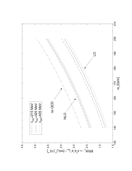
Figure 17: $Br(K_{\rm L}\to\pi^{0}e^{+}e^{-})_{\rm dir}/({\rm Im}\lambda_{t})^{2}$ as a function of $m_{\rm t}$ for various values of $\Lambda_{\overline{\rm MS}}^{(4)}$ at scale $\mu=1.0\,{\rm GeV}$.

The very weak dependence on $\Lambda_{\overline{MS}}$ should be contrasted with the very strong dependence found in the case of $\varepsilon^{\prime}/\varepsilon$. Therefore, provided the other two contributions to $K_{\rm L}\to\pi^{0}e^{+}e^{-}$ can be shown to be small or can be reliably calculated one day, the measurement of $Br(K_{\rm L}\to\pi^{0}e^{+}e^{-})$ should offer a good determination of ${\rm Im}\lambda_{t}$ or $\eta$.

Using the numerical results presented in fig. 17 one finds to a very good approximation:

$$Br(K_{\rm L}\to\pi^{0}e^{+}e^{-})_{\rm dir}=4.9\cdot 10^{-12}\left[\frac{\eta}{0.39}\right]^{2}\left[\frac{|V_{cb}|}{0.040}\right]^{4}\left[\frac{(\overline{m}_{\rm t}(m_{\rm t})}{170\,{\rm GeV}}\right]^{2}\,.$$ (6.16)

Next we would like to comment on the possible uncertainties due to the definition of $m_{\rm t}$. In the formulae above we have set $m_{\rm t}=\overline{m}_{\rm t}(m_{\rm t})$ in accordance with the NLO analysis of CKM parameters in section 4. However, at the level of accuracy at which we work one cannot fully address this question yet. In order to be able to do it, one needs to know the perturbative QCD corrections to $Y_{0}(x_{t})$ and $Z_{0}(x_{t})$ and for consistency an additional order in the renormalization group improved calculation of $P_{0}$. Since the $m_{t}$-dependence of $y_{7V}$ is rather moderate, the main concern in this issue is the coefficient $y_{7A}$ whose $m_{t}$-dependence is fully given by $Y(x_{t})$. Fortunately the QCD corrected function $Y(x_{t})$ is known from the analysis of $K_{\rm L}\to\mu^{+}\mu^{-}$ and can be directly used here. As we will discuss in section 7, for $m_{\rm t}=\overline{m}_{\rm t}(m_{\rm t})$ the QCD corrections to $Y_{0}(x_{t})$ are around 2%. On this basis we believe that if $m_{\rm t}=\overline{m}_{\rm t}(m_{\rm t})$ is chosen, the additional QCD corrections to $Br(K_{\rm L}\to\pi^{0}e^{+}e^{-})_{\rm dir}$ should be small.

Using the input parameters of table 4 and performing two types of error analysis one finds [94]

$$Br(K_{\rm L}\to\pi^{0}e^{+}e^{-})_{\rm dir}=\left\{\begin{array}[]{ll}(4.5\pm 2.6)\cdot 10^{-12}&{\rm Scanning}\\ (4.2\pm 1.4)\cdot 10^{-12}&{\rm Gaussian,}\end{array}\right.$$ (6.17)

where the error comes dominantly from the uncertainties in the CKM parameters. These results are compatible with those found in [50, 132, 141] with differences originating in various choices of CKM parameters and the fact that [94] uses the latest values of $m_{\rm t}$.

Comparing with the estimates of the CP conserving contribution in (6.3) and of the indirectly CP violating contribution in (6.9), we observe that the directly CP violating contribution is comparable to the other two contributions. It is, however, possible that the direct CP violation dominates in this decay (see (6.8)) which is of course very exciting. In order to see whether this is indeed the case improved estimates of the other two contributions are necessary.

Finally it should also be stressed that in reality the CP indirect amplitude may interfere with the vector part of the CP direct amplitude. The full CP violating amplitude can then be written following [139] as follows:

$$Br(K_{\rm L}\to\pi^{0}e^{+}e^{-})_{\rm CP}=|2.43\cdot 10^{-6}re^{i\pi/4}-i\sqrt{\kappa_{e}}Im\lambda_{t}\tilde{y}_{7V}|^{2}+\kappa_{e}(Im\lambda_{t})^{2}\tilde{y}_{7A}^{2}\,.$$ (6.18)

Numerical analyses of (6.18) in [132, 50] show that for $0\leq r\leq 1$ the dependence of $Br(K_{\rm L}\to\pi^{0}e^{+}e^{-})_{\rm CP}$ on $r$ is moderate. It is rather strong otherwise and already for $r<-0.6$ values as high as $10^{-11}$ are found.

6.2.5 Summary and Outlook

The results presented above indicate that within the Standard Model $Br(K_{\rm L}\to\pi^{0}e^{+}e^{-})$ could be as high as $1\cdot 10^{-11}$. Moreover the direct CP violating contribution is found to be important and could even be dominant. Unfortunately the large uncertainties in the remaining two contributions will probably not allow an easy identification of the direct CP violation by measuring the branching ratio only. The future measurements of $Br(K_{\rm S}\to\pi^{0}e^{+}e^{-})$ and improvements in the estimate of the CP conserving part may of course change this unsatisfactory situation. Alternatively the measurements of the electron energy asymmetry [131], [132] and the study of the time evolution of $K^{0}\to\pi^{0}e^{+}e^{-}$ [142], [132], [141] could allow for a refined study of CP violation in this decay.

The present experimental bounds

$$Br(K_{\rm L}\to\pi^{0}e^{+}e^{-})\leq\left\{\begin{array}[]{ll}4.3\cdot 10^{-9}&\cite[cite]{[\@@bibref{}{harris}{}{}]}\\ 5.5\cdot 10^{-9}&\cite[cite]{[\@@bibref{}{ohl}{}{}]}\end{array}\right.$$ (6.19)

are still by three orders of magnitude away from the theoretical expectations in the Standard Model. Yet the prospects of getting the required sensitivity of order $10^{-11}$–$10^{-12}$ by 1999 are encouraging [145]. More details on this interesting decay can be found in the original papers and in the review by Pich [133].

6.3 $B\to X_{s}\gamma$

6.3.1 General Remarks

The rare decay $B\to X_{s}\gamma$ plays an important role in present day phenomenology. The effective Hamiltonian for $B\to X_{s}\gamma$ at scales $\mu={\cal O}(m_{b})$ is given by

$${\cal H}_{\rm eff}(b\to s\gamma)=-\frac{G_{\rm F}}{\sqrt{2}}V_{ts}^{*}V_{tb}\left[\sum_{i=1}^{6}C_{i}(\mu)Q_{i}+C_{7\gamma}(\mu)Q_{7\gamma}+C_{8G}(\mu)Q_{8G}\right]\,,$$ (6.20)

where in view of $\mid V_{us}^{*}V_{ub}/V_{ts}^{*}V_{tb}\mid<0.02$ we have neglected the term proportional to $V_{us}^{*}V_{ub}$. Here $Q_{1}....Q_{6}$ are the usual four-fermion operators whose explicit form is given in (2.61-2.63). The remaining two operators, characteristic for this decay, are the Magnetic–Penguins

$$Q_{7\gamma}=\frac{e}{8\pi^{2}}m_{b}\bar{s}_{\alpha}\sigma^{\mu\nu}(1+\gamma_{5})b_{\alpha}F_{\mu\nu},\qquad Q_{8G}=\frac{g}{8\pi^{2}}m_{b}\bar{s}_{\alpha}\sigma^{\mu\nu}(1+\gamma_{5})T^{a}_{\alpha\beta}b_{\beta}G^{a}_{\mu\nu}$$ (6.21)

originating in the diagrams of fig. 11d. In order to derive the contribution of $Q_{7\gamma}$ to the Hamiltonian in (6.20), in the absence of QCD corrections, one multiplies the vertex in (2.21) by “i” and makes the replacement

$$2i\sigma_{\mu\nu}q^{\nu}\to-\sigma^{\mu\nu}F_{\mu\nu}.$$ (6.22)

Analogous procedure gives the contribution of $Q_{8G}$.

It is the magnetic $\gamma$-penguin which plays the crucial role in this decay. However, the role of the dominant current-current operator $Q_{2}$ should not be underestimated. Indeed the perturbative QCD effects involving in particular the mixing between $Q_{2}$ and $Q_{7\gamma}$ are very important in this decay. They are known [146, 147] to enhance $C_{7\gamma}(\mu)$ for $\mu={\cal O}(m_{b})$ substantially, so that the resulting branching ratio $Br(B\to X_{s}\gamma)$ turns out to be by a factor of 2–3 higher than it would be without QCD effects. Since the first analyses in [146, 147] a lot of progress has been made in calculating these important QCD effects beginning with the work in [148, 149]. We will briefly summarize this progress.

A peculiar feature of the renormalization group analysis in $B\to X_{s}\gamma$ is that the mixing under infinite renormalization between the set $(Q_{1}...Q_{6})$ and the operators $(Q_{7\gamma},Q_{8G})$ vanishes at the one-loop level. Consequently in order to calculate the coefficients $C_{7\gamma}(\mu)$ and $C_{8G}(\mu)$ in the leading logarithmic approximation, two-loop calculations of ${\cal{O}}(eg^{2}_{s})$ and ${\cal{O}}(g^{3}_{s})$ are necessary. The corresponding NLO analysis requires the evaluation of the mixing in question at the three-loop level. This peculiar feature caused that the first fully correct calculation of the leading anomalous dimension matrix relevant for this decay has been obtained only in 1993 [150, 151]. It has been confirmed subsequently in [152, 153, 51].

In 1996 the NLO corrections have been completed. It was a joint effort of many groups. The two-loop mixing involving the operators $Q_{1}.....Q_{6}$ and the two-loop mixing in the sector $(Q_{7\gamma},Q_{8G})$ has been calculated in [33, 34, 35, 23, 37, 38] and [39], respectively. The $O(\alpha_{s})$ corrections to $C_{7\gamma}(M_{W})$ and $C_{8G}(M_{W})$ have been first calculated in [54] and recently confirmed in [58]. One-loop matrix elements $\langle s\gamma{\rm gluon}|Q_{i}|b\rangle$ have been calculated in [53, 55]. The very difficult two-loop corrections to $\langle s\gamma|Q_{i}|b\rangle$ have been presented in [56]. Finally after a heroic effort the three loop mixing between the set $(Q_{1}...Q_{6})$ and the operators $(Q_{7\gamma},Q_{8G})$ has been completed at the end of 1996 [57]. As a byproduct the authors of [57] confirmed the existing two-loop anomalous dimension matrix in the $Q_{1}...Q_{6}$ sector.

In order to appreciate the importance of NLO calculations for this decay it is instructive to discuss first the leading logarithmic approximation.

6.3.2 The Decay $B\to X_{s}\gamma$ in the Leading Log Approximation

In calculating $Br(B\to X_{s}\gamma)$ it is customary to use the spectator model in which the inclusive decay $B\to X_{s}\gamma$ is approximated by the partonic decay $b\to s\gamma$. That is one uses the following approximate equality:

$$\frac{\Gamma(B\to X_{s}\gamma)}{\Gamma(B\to X_{c}e\bar{\nu}_{e})}\simeq\frac{\Gamma(b\to s\gamma)}{\Gamma(b\to ce\bar{\nu}_{e})}\equiv R_{{\rm quark}},$$ (6.23)

where the quantities on the r.h.s are calculated in the spectator model corrected for short-distance QCD effects. The normalization to the semileptonic rate is usually introduced in order to cancel the uncertainties due to the CKM matrix elements and factors of $m_{\rm b}^{5}$ in the r.h.s. of (6.23). Additional support for the approximation given above comes from the heavy quark expansions. Indeed the spectator model has been shown to correspond to the leading order approximation of an expansion in $1/m_{\rm b}$. The first corrections appear at the ${\cal O}(1/m_{\rm b}^{2})$ level and will be discussed at the end of this section.

The leading logarithmic calculations [148, 151, 152, 51, 154, 155] can be summarized in a compact form as follows:

$$R_{{\rm quark}}=\frac{|V_{ts}^{*}V_{tb}|^{2}}{|V_{cb}|^{2}}\frac{6\alpha}{\pi f(z)}|C^{(0){\rm eff}}_{7\gamma}(\mu)|^{2}\,,$$ (6.24)

where

$$f(z)=1-8z^{2}+8z^{6}-z^{8}-24z^{4}\ln z\quad\mbox{with}\quad z=\frac{m_{\rm c}}{m_{\rm b}}$$ (6.25)

is the phase space factor in the semileptonic $b$-decay.

The crucial quantity in (6.24) is the effective coefficient $C^{(0){\rm eff}}_{7\gamma}(\mu)$ given explicitly as follows:

$$C_{7\gamma}^{(0){\rm eff}}(\mu)=\eta^{\frac{16}{23}}C_{7\gamma}^{(0)}(M_{\rm W})+\frac{8}{3}\left(\eta^{\frac{14}{23}}-\eta^{\frac{16}{23}}\right)C_{8G}^{(0)}(M_{\rm W})+C_{2}^{(0)}(M_{\rm W})\sum_{i=1}^{8}h_{i}\eta^{a_{i}}\,,$$ (6.26)

where

$$C^{(0)}_{2}(M_{\rm W})=1$$ (6.27)

$$C^{(0)}_{7\gamma}(M_{\rm W})=\frac{3x_{t}^{3}-2x_{t}^{2}}{4(x_{t}-1)^{4}}\ln x_{t}+\frac{-8x_{t}^{3}-5x_{t}^{2}+7x_{t}}{24(x_{t}-1)^{3}}\equiv-\frac{1}{2}D^{\prime}_{0}(x_{t})$$ (6.28)

and

$$\eta=\frac{\alpha_{s}(M_{\rm W})}{\alpha_{s}(\mu)}.$$ (6.29)

For completeness we give also

$$C_{8G}^{(0){\rm eff}}(\mu)=\eta^{\frac{14}{23}}C_{8G}^{(0)}(M_{\rm W})+C_{2}^{(0)}(M_{\rm W})\sum_{i=1}^{8}\bar{h}_{i}\eta^{a_{i}},$$ (6.30)

which is relevant for $b\to s~{}{\rm gluon}$ transition. Here

$$C^{(0)}_{8G}(M_{\rm W})=\frac{-3x_{t}^{2}}{4(x_{t}-1)^{4}}\ln x_{t}+\frac{-x_{t}^{3}+5x_{t}^{2}+2x_{t}}{8(x_{t}-1)^{3}}\equiv-\frac{1}{2}E^{\prime}_{0}(x_{t}).$$ (6.31)

The functions $D^{\prime}_{0}(x_{t})$ and $E^{\prime}_{0}(x_{t})$ appeared already in section 2. The numbers $a_{i}$, $h_{i}$ and $\bar{h}_{i}$ are given in table 12.

$i$	1	2	3	4	5	6	7	8
$a_{i}$	$\frac{14}{23}$	$\frac{16}{23}$	$\frac{6}{23}$	$-\frac{12}{23}$	$0.4086$	$-0.4230$	$-0.8994$	$0.1456$
$h_{i}$	$2.2996$	$-1.0880$	$-\frac{3}{7}$	$-\frac{1}{14}$	$-0.6494$	$-0.0380$	$-0.0185$	$-0.0057$
$\bar{h}_{i}$	$0.8623$	$0$	$0$	$0$	$-0.9135$	$0.0873$	$-0.0571$	$0.0209$

Table 12: Magic Numbers.

Using the leading $\mu$-dependence of $\alpha_{s}$:

$$\alpha_{s}(\mu)=\frac{\alpha_{s}(M_{\rm Z})}{1-\beta_{0}\alpha_{s}(M_{\rm Z})/2\pi\,\ln(M_{\rm Z}/\mu)}$$ (6.32)

one finds the results in table 13.

	$\alpha_{s}^{(5)}(M_{\rm Z})=0.113$		$\alpha_{s}^{(5)}(M_{\rm Z})=0.118$		$\alpha_{s}^{(5)}(M_{\rm Z})=0.123$
$\mu[\,{\rm GeV}]$	$C^{(0){\rm eff}}_{7\gamma}$	$C^{(0){\rm eff}}_{8G}$	$C^{(0){\rm eff}}_{7\gamma}$	$C^{(0){\rm eff}}_{8G}$	$C^{(0){\rm eff}}_{7\gamma}$	$C^{(0){\rm eff}}_{8G}$
2.5	–0.328	–0.155	–0.336	–0.158	–0.344	–0.161
5.0	–0.295	–0.142	–0.300	–0.144	–0.306	–0.146
7.5	–0.277	–0.134	–0.282	–0.136	–0.286	–0.138
10.0	–0.265	–0.130	–0.269	–0.131	–0.273	–0.133

Table 13: Wilson coefficients $C^{(0){\rm eff}}_{7\gamma}$ and $C^{(0){\rm eff}}_{8G}$ for $m_{\rm t}=170\,{\rm GeV}$ and various values of $\alpha_{s}^{(5)}(M_{\rm Z})$ and $\mu$.

Two features of these results should be emphasised:

• The strong enhancement of the coefficient $C^{(0){\rm eff}}_{7\gamma}$ by short distance QCD effects which we illustrate by the relative numerical importance of the three terms in expression (6.26). For instance, for $m_{\rm t}=170\,{\rm GeV}$, $\mu=5\,{\rm GeV}$ and $\alpha_{s}^{(5)}(M_{\rm Z})=0.118$ one obtains

  $$C^{(0){\rm eff}}_{7\gamma}(\mu) = 0.695\;C^{(0)}_{7\gamma}(M_{\rm W})+0.085\;C^{(0)}_{8G}(M_{\rm W})-0.158\;C^{(0)}_{2}(M_{\rm W})$$ (6.33)

  $$= 0.695\;(-0.193)+0.085\;(-0.096)-0.158=-0.300\,.$$

  In the absence of QCD we would have $C^{(0){\rm eff}}_{7\gamma}(\mu)=C^{(0)}_{7\gamma}(M_{\rm W})$ (in that case one has $\eta=1$). Therefore, the dominant term in the above expression (the one proportional to $C^{(0)}_{2}(M_{\rm W})$) is the additive QCD correction that causes the enormous QCD enhancement of the $B\to X_{s}\gamma$ rate [146, 147]. It originates solely from the two-loop diagrams. On the other hand, the multiplicative QCD correction (the factor 0.695 above) tends to suppress the rate, but fails in the competition with the additive contributions.

  In the case of $C^{(0){\rm eff}}_{8G}$ a similar enhancement is observed

  $$C^{(0){\rm eff}}_{8G}(\mu) = 0.727\;C^{(0)}_{8G}(M_{\rm W})-0.074\;C^{(0)}_{2}(M_{\rm W})$$ (6.34)

  $$= 0.727\;(-0.096)-0.074=-0.144\,.$$

• A strong $\mu$-dependence of both coefficients as first stressed by Ali and Greub [154] and confirmed in [155]. One can see that when $\mu$ is varied by a factor of 2 in both directions around $m_{\rm b}\simeq 5\,{\rm GeV}$, the ratio (6.24) changes by around $\pm 25\%$, i.e. the ratios $R_{{\rm quark}}$ obtained for $\mu=2.5\,{\rm GeV}$ and $\mu=10\,{\rm GeV}$ differ by a factor of 1.6 [154]. Since $B\to X_{s}\gamma$ is dominated by QCD effects, it is not surprising that this scale-uncertainty in the leading order is particularly large.

A critical analysis of theoretical and experimental uncertainties present in the prediction for Br($B\to X_{s}\gamma$ ) based on the formula (6.24) has been made in [155] giving

$$Br(B\to X_{s}\gamma)_{{\rm TH}}=(2.8\pm 0.8)\times 10^{-4}$$ (6.35)

where the error is dominated by the uncertainty in the choice of the renormalization scale $m_{b}/2<\mu<2m_{b}$ discussed above. To this end $Br(B\to X_{c}e\bar{\nu}_{e})=(10.43\pm 0.24)\%$ has been used. Similar result has been found in [154].

In 1994 the first measurement of the inclusive rate was presented by CLEO [156]:

$$Br(B\to X_{s}\gamma)=(2.32\pm 0.57\pm 0.35)\times 10^{-4}\,,$$ (6.36)

where the first error is statistical and the second is systematic. We will report on the status of the exclusive measurements such as $B\to K^{*}\gamma$ later on.

The result in (6.36) agrees with (6.35) although the large theoretical and experimental errors do not allow for a definitive conclusion and to see whether some contributions beyond the Standard Model, such as present in the Two-Higgs-Doublet Model (2HDM) or in the Minimal Supersymmetric Standard Model (MSSM), are required. In any case the agreement of the theory with data is consistent with the large QCD enhancement of $B\to X_{s}\gamma$ . Without this enhancement the theoretical prediction would be at least by a factor of 2 below the data.

Since the theoretical result in (6.35) is dominated by the scale ambiguities present in the leading order approximation, it was clear already in 1993 that a complete NLO analysis is very desirable. Such a complete next-to-leading calculation of $B\to X_{s}\gamma$ was described in [155] in general terms. As demonstrated formally there, the cancellation of the dominant $\mu$-dependence in the leading order can then be achieved. While this formal NLO analysis was very encouraging with respect to the reduction of the $\mu$-dependence, it could obviously not provide the actual size of Br($B\to X_{s}\gamma$ ) after the inclusion of NLO corrections. Fortunately three years later such a complete NLO analysis exists and the impact of NLO corrections on Br($B\to X_{s}\gamma$ ) can be analysed in explicit terms.

6.3.3 $B\to X_{s}\gamma$ Beyond Leading Logarithms

The formula (6.24) modifies after the inclusion of NLO corrections as follows [57]:

$$R_{{\rm quark}}=\frac{|V_{ts}^{*}V_{tb}|^{2}}{|V_{cb}|^{2}}\frac{6\alpha}{\pi f(z)}F\left(|D|^{2}+A\right)\,,$$ (6.37)

where

$$F=\frac{1}{\kappa(z)}\left(\frac{m_{b}(\mu=m_{b})}{m_{b,{\rm pole}}}\right)^{2}=\frac{1}{\kappa(z)}\left(1-\frac{8}{3}\frac{\alpha_{s}(m_{b})}{\pi}\right),$$ (6.38)

$$D=C_{7\gamma}^{(0){\rm eff}}(\mu_{b})+\frac{\alpha_{s}(\mu_{b})}{4\pi}\left\{C_{7\gamma}^{(1){\rm eff}}(\mu_{b})+\sum_{i=1}^{8}C_{i}^{(0){\rm eff}}(\mu_{b})\left[r_{i}+\gamma_{i7}^{(0){\rm eff}}\ln\frac{m_{b}}{\mu_{b}}\right]\right\}$$ (6.39)

and $A$ is discussed below. Here $\mu_{b}={\cal O}(m_{b})$.

We will now explain the origin of various new contributions:

• First $\kappa(z)$ is the QCD correction to the semileptonic decay [157]. To a good approximation it is given by [158]

  $$\kappa(z)=1-\frac{2\alpha_{s}(m_{b})}{3\pi}\left[(\pi^{2}-\frac{31}{4})(1-z)^{2}+\frac{3}{2}\right]\,.$$ (6.40)

  An exact analytic formula for $\kappa(z)$ can be found in [159].

• The second factor in (6.38) originates as follows. The $B\to X_{s}\gamma$ rate is proportional to $m_{b,{\rm pole}}^{3}$ present in the two body phase space and to $m_{b}(\mu=m_{b})^{2}$ present in $<s\gamma|Q_{7\gamma}|B>^{2}$. On the other hand the semileptonic rate is is proportional to $m_{b,{\rm pole}}^{5}$ present in the three body phase space. Thus the $m_{b}^{5}$ factors present in both rates differ by a ${\cal O}(\alpha_{s})$ correction which has been consistently omitted in the leading logarithmic approximation.

• For similar reason the variable $z$ entering $f(z)$ and $\kappa(z)$ can be more precisely specified at the NLO level to be [56, 57]:

  $$z=\frac{m_{c,{\rm pole}}}{m_{b,{\rm pole}}}=0.29\pm 0.02$$ (6.41)

  which is obtained from $m_{b,{\rm pole}}=4.8\pm 0.15$ GeV and $m_{b,{\rm pole}}-m_{c,{\rm pole}}=3.40$ GeV. This gives

  $$\kappa(z)=0.879\pm 0.002\approx 0.88\,,\qquad f(z)=0.54\pm 0.04\,.$$ (6.42)

• The amplitude $D$ in (6.39) includes two types of new contributions. The first $\alpha_{s}$-correction originates in the NLO correction to the Wilson coefficients of $Q_{7\gamma}$:

  $$C^{\rm eff}_{7\gamma}(\mu)=C^{(0){\rm eff}}_{7\gamma}(\mu)+\frac{\alpha_{s}(\mu)}{4\pi}C^{(1){\rm eff}}_{7\gamma}(\mu)\,.$$ (6.43)

  It is this correction which requires the calculation of the three-loop anomalous dimensions [57]. An explicit formula for $C^{(1){\rm eff}}_{7\gamma}(\mu)$ can be found in [57]. It has a similar structure to (6.26) with $C_{7\gamma}^{(0)}(M_{\rm W})$ and $C_{8G}^{(0)}(M_{\rm W})$ replaced by the corresponding NLO corrections calculated in [54, 58]. Also the $C_{2}(M_{\rm W})$-part in (6.26) has to be modified.

  The two remaining corrections in (6.39) come from one-loop matrix elements $<s\gamma|Q_{7\gamma}|B>$ and $<s\gamma|Q_{8G}|B>$ and from two-loop matrix elements $<s\gamma|Q_{i}|B>$ of the remaining operators. These two-loop matrix elements have been calculated in [56]. The coefficients of the logarithm are the relevant elements in the leading anomalous dimension matrix. The explicit logarithmic $\mu_{b}$ dependence in the last term in $D$ cancels the leading $\mu_{b}$ dependence present in the first term in (6.39) as already pointed out in [155].

  Now $C^{(1){\rm eff}}_{7\gamma}(\mu)$ is renormalization scheme dependent. This scheme dependence is cancelled by the one present in the constant terms $r_{i}$. Actually ref. [56] does not provide the matrix elements of the QCD-penguin operators and consequently $r_{i}~{}(i=3-6)$ are unknown. However, the Wilson coefficients of QCD-penguin operators are very small and this omission is immaterial.

• The term $A$ in (6.37) originates from the bremsstrahlung corrections and the necessary virtual corrections needed for the cancellation of the infrared divergences. These have been calculated in [53, 55] and are also considered in [57, 56] in the context of the full analysis. Since the virtual corrections are also present in the terms $r_{i}$ in $D$, care must be taken in order to avoid double counting. This is discussed in detail in [57] where an explicit formula for $A$ can be found. Actually $A$ depends on an explicit lower cut on the photon energy

  $$E_{\gamma}>(1-\delta)E_{\gamma}^{{\rm max}}\equiv(1-\delta)\frac{m_{b}}{2}.$$ (6.44)

  Moreover $A$ is divergent in the limit $\delta\to 1$. In order to cancel this divergence one would have to consider the sum of $B\to X_{s}\gamma$ and $b{\to}X_{s}$ decay rates. However, the divergence at $\delta{\to}1$ is very slow. In order to allow an easy comparison with previous experimental and theoretical publications the authors in [57] choose $\delta=0.99$. Further details on the $\delta$-dependence can be found in this paper.

• Finally the values of $\alpha_{s}(\mu)$ in all the above formulae are calculated with the use of the NLO expression for the strong coupling constant:

  $$\alpha_{s}(\mu)=\frac{\alpha_{s}(M_{Z})}{v(\mu)}\left[1-\frac{\beta_{1}}{\beta_{0}}\frac{\alpha_{s}(M_{Z})}{4\pi}\frac{\ln v(\mu)}{v(\mu)}\right],$$ (6.45)

  where

  $$v(\mu)=1-\beta_{0}\frac{\alpha_{s}(M_{Z})}{2\pi}\ln\left(\frac{M_{Z}}{\mu}\right),$$ (6.46)

  $\beta_{0}=\frac{23}{3}$ and $\beta_{1}=\frac{116}{3}$.

The main uncertainty in the leading order formulae related to the $\mu$-dependence has been thus considerably reduced at the NLO level. This reduction comes dominantly through the inclusion of the two-loop matrix element of the operator $Q_{2}$ calculated in [56]. However, as we stated above, the calculation of the three loop anomalous dimensions present in $C^{(1){\rm eff}}_{7\gamma}(\mu)$ is necessary for the complete analysis and in particular for the cancellation of the renormalization scheme dependence. As analysed in [56, 57] the $\mu$ dependence in the final result for Br($B\to X_{s}\gamma$ ) is reduced from $\pm 25\%$ in LO down to $\pm 6\%$. Other sources of uncertainties are given in table 14 taken from [57]. We observe that the dominant sources of remaining uncertainties are $m_{c}/m_{b}$ and $\mu_{b}$.

$\alpha_{s}(M_{Z})$	$m_{t}$	$\mu_{b}$	$m_{c,{\rm pole}}/m_{b,{\rm pole}}$	$m_{b,{\rm pole}}$	$\alpha$	CKM angles
2.5%	1.7%	6.2%	5.2%	0.5%	1.9%	2.1%

Table 14: Uncertainties in $R_{{\rm quark}}$ due to various sources.

Finally one has to pass from the calculated $b$-quark decay rates to the $B$-meson decay rates. Relying on the Heavy Quark Expansion (HQE) calculations one finds [57]

$$Br(B{\to}X_{s}\gamma)=Br(B{\to}X_{c}e\bar{\nu_{e}})\cdot R_{{\rm quark}}\left(1-\frac{\delta^{NP}_{sl}}{m_{b}^{2}}+\frac{\delta^{NP}_{rad}}{m_{b}^{2}}\right),$$ (6.47)

where $\delta^{{\rm NP}}_{{\rm sl}}$ and $\delta^{{\rm NP}}_{{\rm rad}}$ parametrize nonperturbative corrections to the semileptonic and radiative $B$-meson decay rates, respectively.

According to [160], $\delta^{{\rm NP}}_{{\rm sl}}=-(1.05\pm 0.10)\;{\rm GeV}^{2}$. Next, following [161], one can express $\delta^{{\rm NP}}_{{\rm rad}}$ in terms of the HQET parameters $\lambda_{1}$ and $\lambda_{2}$:

$$\delta^{{\rm NP}}_{{\rm rad}}=\frac{1}{2}\lambda_{1}-\frac{9}{2}\lambda_{2}.$$ (6.48)

The value of $\lambda_{2}$ is known from $B^{*}$–$B$ mass splitting

$$\lambda_{2}=\frac{1}{4}(m_{B^{*}}^{2}-m_{B}^{2})\simeq 0.12\;{\rm GeV}^{2}.$$ (6.49)

The value of $\lambda_{1}$ is controversial. In [57], $\lambda_{1}=-(0.6\pm 0.1)\;{\rm GeV}^{2}$ taken from [160] has been used.

The two nonperturbative corrections in (6.47) are both around $4\%$ in magnitude and tend to cancel each other. In effect, they sum up to only $(1\pm 0.5)\%$. As stressed in [57], such a small number has to be taken with caution. If values of $\lambda_{1}$ around $-0.1\;{\rm GeV}^{2}$ were accepted [161], the total nonperturbative correction in (6.47) would change by one or two percent. Moreover, one has to remember that the four-quark operators $Q_{1}......Q_{6}$ have not been included in the calculation of $\delta^{{\rm NP}}_{{\rm rad}}$. Contributions from these operators could potentially give one- or two-percent effects. Nevertheless, it seems reasonable to conclude that the total nonperturbative $1/m_{b}^{2}$ correction to (6.47) is well below 10%, i.e. it is smaller than the inaccuracy of the perturbative calculation of $R_{{\rm quark}}$.

Using $Br(B{\to}X_{c}e\bar{\nu_{e}})=(10.4\pm 0.4)\%$ [60], the authors of [57] find the following prediction for $Br(B{\to}X_{s}\gamma)$ :

$$Br(B{\to}X_{s}\gamma)=(3.28\pm 0.33)\times 10^{-4}.$$ (6.50)

Similar result has been obtained in [56]. Comparing with the leading order estimate (6.35) we observe that the central value has been shifted upwards by roughly $15\%$ and the theoretical uncertainty has been reduced by more than a factor of two. We also note that the central value of the NLO prediction is outside the $1\sigma$ experimental error bar in (6.36). However, the experimental and theoretical error bars practically touch each other. Therefore we conclude that the present $B{\to}X_{s}\gamma$ measurement remains in agreement with the Standard Model.

6.3.4 Long Distance Contributions

The long distance contributions to $B\to X_{s}\gamma$ are not easy to calculate and the present estimates are based on phenomenological models. These long distance contributions are expected to arise dominantly from transitions $B\to\sum_{i}V_{i}+X_{s}\to\gamma X_{s}$ where $V_{i}=J/\psi,\psi^{\prime},...$. In view of space limitations we will not discuss these contributions which are generally expected to be below $10\%$ [162]. A better estimate of these effects is desirable.

A related issue are the ${\cal O}(1/m^{2}_{c})$ corrections pointed out recently by Voloshin [163] and also discussed by other authors [164]. These non-perturbative corrections originate in the photon coupling to a virtual $c\bar{c}$ loop and their general structure is given by

$$(\Lambda_{\rm QCD}^{2}/m_{\rm c}^{2})(\Lambda_{\rm QCD}m_{\rm b}/m_{\rm c}^{2})^{n}$$

with $(n=0,1..)$. The term $n=0$ can be estimated reliably and amounts to a $3\%$ reduction of the rate. Since $\Lambda_{\rm QCD}m_{\rm b}/m_{\rm c}^{2}\approx 0.6$, the terms with $n>0$ are not necessarily much smaller. Although the presence of unknown matrix elements in these contributions does not allow a definite estimate of their actual size, the analyses in [164] indicate, however, that these higer order contributions are substantially smaller than the $n=0$ term. Less optimistic view can be found in [163].

6.3.5 $B\to K^{*}\gamma$ and other Exclusive Modes

In 1993 CLEO reported [165] $Br(B\to K^{*}\gamma)=(4.5\pm 1.5\pm 0.9)\times 10^{-5}.$ This was in fact the first observation of the $b\to s\gamma$ transition and equivalently of magnetic $\gamma$-penguins. The corresponding 1996 value has a substantially smaller error [166]:

$$Br(B\to K^{*}\gamma)=(4.2\pm 0.8\pm 0.6)\times 10^{-5}$$ (6.51)

implying an improved measurement of $R_{K^{*}}$:

$$R_{K^{*}}=\frac{\Gamma(B\to K^{*}\gamma)}{\Gamma(B\to X_{s}\gamma)}=0.181\pm 0.068$$ (6.52)

This result puts some constraints on various formfactor models listed in [166]. There one can also find 90% C.L. bounds: $Br(B^{0}\to\rho^{0}\gamma)<3.9\cdot 10^{-5}$, $Br(B^{0}\to\omega\gamma)<1.3\cdot 10^{-5}$, $Br(B^{-}\to\rho^{-}\gamma)<1.1\cdot 10^{-5}$. Combined with (6.51) these bounds imply

$$\frac{|V_{td}|}{|V_{ts}|}\leq 0.45-0.56\,,$$ (6.53)

where the uncertainty in the bound reflects the model dependence. Clearly this bound is still higher by a factor of two than the value obtained in the standard analysis of section 4. In 1996 also DELPHI [167] provided two bounds: $Br(B^{0}_{d}\to K^{*}\gamma)<2.1\cdot 10^{-4}$ and $Br(B^{0}_{s}\to\phi\gamma)<7.0\cdot 10^{-4}$. The second bound is the only existing bound on this decay.

6.3.6 Summary and Outlook

The rare decay $B\to X_{s}\gamma$ plays at present together with $B^{0}_{d,s}-\bar{B}^{0}_{d,s}$ mixing the central role in loop induced transitions in the $B$-system. On the theoretical side considerable progress has been made last year by calculating NLO corrections, thereby reducing the large $\mu_{b}$ uncertainties present in the leading order. This way the error in the short distance prediction for $Br(B\to X_{s}\gamma)$ as given in (6.50) has been decreased down to roughly $\pm 10\%$ compared with $\pm(25-30)\%$ in the leading order. The precise size of long distance contributions due to the intermediate $J/\psi$ state is difficult to obtain but generally these contributions are found to be below $10\%$. The $1/m_{b}^{2}$ and $1/m_{c}^{2}$ corrections amount to a few percent.

On the experimental side considerable progress has been made by CLEO in the case of $Br(B^{0}_{d}\to K^{*}\gamma)$. It is very desirable to obtain now an improved measurement of $Br(B\to X_{s}\gamma)$. As advertised at the HEP conference in Warsaw by Browder, Kagan and Kagan, CLEO II should be able to discover $b\to s~{}{\rm gluon}$ transition soon. In view of this and the fact that here the theoretical uncertainties are large, theorists should sharpen their tools.

More on $B\to X_{s}\gamma$ , in particular on the photon spectrum and the determination of $|V_{td}|/|V_{ts}|$ from $B\to X_{s,d}\gamma$, can be found in [95, 168, 169]. The impact of new physics is discussed in another chapter of this book [170]. CP violation in $B\to K^{*}\gamma$ and $B\to\varrho\gamma$ is discussed in [171].

6.4 $B\to X_{s}l^{+}l^{-}$

6.4.1 General Remarks

The rare decays $B\to X_{s}l^{+}l^{-}$ have been the subject of many theoretical studies in the framework of the Standard Model and its extensions such as the two Higgs doublet models and models involving supersymmetry [173]-[181]. In particular the strong dependence of $B\to X_{s}l^{+}l^{-}$ on $m_{\rm t}$ has been stressed in [173]. It is clear that once these decays have been observed, they will offer a useful test of the Standard Model and its extensions. We will concentrate here on the predictions within the Standard Model and in particular on $B\to X_{s}\mu^{+}\mu^{-}$. The impact of new physics is discussed in another chapter in this book [170].

The central element in any analysis of $B\to X_{s}\mu^{+}\mu^{-}$ is the effective Hamiltonian at scales $\mu=O(m_{b})$ given by

$${\cal H}_{\rm eff}(b\to s\mu^{+}\mu^{-})={\cal H}_{\rm eff}(b\to s\gamma)-\frac{G_{\rm F}}{\sqrt{2}}V_{ts}^{*}V_{tb}\left[C_{9V}(\mu)Q_{9V}+C_{10A}(M_{W})Q_{10A}\right]\,,$$ (6.54)

where we have again neglected the term proportional to $V_{us}^{*}V_{ub}$ and ${\cal H}_{\rm eff}(b\to s\gamma)$ is given in (6.20). In addition to the operators relevant for $B\to X_{s}\gamma$, there are two new operators:

$$Q_{9V}=(\bar{s}b)_{V-A}(\bar{\mu}\mu)_{V}\,,\qquad Q_{10A}=(\bar{s}b)_{V-A}(\bar{\mu}\mu)_{A}\,,$$ (6.55)

where $V$ and $A$ refer to $\gamma_{\mu}$ and $\gamma_{\mu}\gamma_{5}$, respectively. They are generated through the electroweak penguin diagrams of fig. 11f and the related box diagrams needed mainly to keep gauge invariance.

The actual calculation of $Br(B\to X_{s}\mu^{+}\mu^{-})$ involves the evaluation of the Wilson coefficients of the relevant local operators and the calculation of the corresponding matrix elements of these operators relevant for the decay in question. As in the case of $B\to X_{s}\gamma$, the latter part of the analysis can be done in the spectator model which, as indicated by the heavy quark expansion, should offer a good approximation to QCD for $B$-decays. One can also include the non-perturbative ${\cal O}(1/m_{\rm b}^{2})$ corrections to the spectator model which we will briefly discuss at the end of this section. A realistic phenomenological analysis should also include the long-distance contributions which are mainly due to the $J/\psi$ and $\psi^{\prime}$ resonances [182]-[187]. We will first concentrate our presentation on the short distance contributions. The impact of the long distance contributions will be briefly discussed subsequently.

6.4.2 Wilson Coefficients $C_{9V}(\mu)$ and $C_{10A}(\mu)$

The coefficient $C_{10A}(\mu)$ is given by

$$C_{10A}(M_{\rm W})=\frac{\alpha}{2\pi}\tilde{C}_{10}(M_{\rm W}),\qquad\tilde{C}_{10}(M_{\rm W})=-\frac{Y_{0}(x_{t})}{\sin^{2}\Theta_{\rm W}}$$ (6.56)

with $Y_{0}(x)$ given in (2.78). Since $Q_{10A}$ does not renormalize under QCD, its coefficient does not depend on $\mu\approx{\cal O}(m_{\rm b})$. The only renormalization scale dependence in (6.56) enters through the definition of the top quark mass. We will return to this issue below.

The main issue of QCD corrections to $B\to X_{s}\mu^{+}\mu^{-}$ centers around the coefficient $C_{9V}(\mu)$. The special feature of $C_{9V}(\mu)$ compared to the coefficients of the remaining operators contributing to $B\to X_{s}\mu^{+}\mu^{-}$ is the large logarithm represented by $1/\alpha_{s}$ in $P_{0}$ in the formula (6.59) given below. Consequently the renormalization group improved perturbation theory for $C_{9V}$ has the structure ${\cal O}(1/\alpha_{s})+{\cal O}(1)+{\cal O}(\alpha_{s})+\ldots$ whereas the corresponding series for the remaining coefficients is ${\cal O}(1)+{\cal O}(\alpha_{s})+\ldots$. Therefore in order to find the next-to-leading ${\cal O}(1)$ term in the branching ratio for $B\to X_{s}\mu^{+}\mu^{-}$, the full two-loop renormalization group analysis has to be performed in order to find $C_{9V}$, but the coefficients of the remaining operators should be taken in the leading logarithmic approximation. In particular at the NLO level one should only include the leading term $C^{(0){\rm eff}}_{7\gamma}(\mu)$ in (6.43). The recently calculated scheme dependent correction $C^{(1){\rm eff}}_{7\gamma}(\mu)$ is a part of next-to-NLO correction to $B\to X_{s}\mu\bar{\mu}$ and should be omitted in a consistent NLO calculation.

The QCD corrections to $C_{9V}(\mu)$ have been calculated over the last years with increasing precision by several groups [174, 188, 189, 51] culminating in two complete next-to-leading QCD calculations [51, 52] which agree with each other. Defining $\tilde{C}_{9}$ by

$$C_{9V}(\mu)=\frac{\alpha}{2\pi}\tilde{C}_{9}(\mu)$$ (6.57)

one finds [52] in the NDR scheme

$$\tilde{C}_{9}^{\rm NDR}(\mu)=P_{0}^{\rm NDR}+\frac{Y_{0}(x_{t})}{\sin^{2}\Theta_{\rm W}}-4Z_{0}(x_{t})+P_{E}E_{0}(x_{t})$$ (6.58)

with

$$P_{0}^{\rm NDR} = \frac{\pi}{\alpha_{s}(M_{\rm W})}(-0.1875+\sum_{i=1}^{8}p_{i}\eta^{a_{i}+1})$$ (6.59)

$$+1.2468+\sum_{i=1}^{8}\eta^{a_{i}}[r^{\rm NDR}_{i}+s_{i}\eta]$$

$$P_{E} = 0.1405+\sum_{i=1}^{8}q_{i}\eta^{a_{i}+1}\,.$$ (6.60)

The formula (6.58) has an identical structure to (6.14) relevant for $K_{\rm L}\to\pi^{0}e^{+}e^{-}$ with different numerical values for $P_{0}$ and $P_{E}$ due to different scales $\mu$ involved. However, because of the one step evolution from $\mu=M_{\rm W}$ down to $\mu=m_{\rm b}$ without the charm threshold in between, it was possible to find an analytic formula for $P_{0}$ here which was not possible in the case of $K_{\rm L}\to\pi^{0}e^{+}e^{-}$.

$Y_{0}(x)$, $Z_{0}(x)$ and $E_{0}(x)$ are defined in (2.78), (2.79) and (2.27), respectively. The powers $a_{i}$ are the same as in table 12. The coefficients $p_{i}$, $r^{\rm NDR}_{i}$, $s_{i}$, and $q_{i}$ can be found in table 15. $P_{E}$ is ${\cal O}(10^{-2})$ and consequently the last term in (6.58) can be neglected. We keep it however in our numerical analysis.

$i$	1	2	3	4	5	6	7	8
$p_{i}$	$0,$	$0,$	$-\frac{80}{203},$	$\frac{8}{33},$	$0.0433$	$0.1384$	$0.1648$	$-0.0073$
$r^{\rm NDR}_{i}$	$0$	$0$	$0.8966$	$-0.1960$	$-0.2011$	$0.1328$	$-0.0292$	$-0.1858$
$s_{i}$	$0$	$0$	$-0.2009$	$-0.3579$	$0.0490$	$-0.3616$	$-0.3554$	$0.0072$
$q_{i}$	$0$	$0$	$0$	$0$	$0.0318$	$0.0918$	$-0.2700$	$0.0059$
$r^{\rm HV}_{i}$	$0$	$0$	$-0.1193$	$0.1003$	$-0.0473$	$0.2323$	$-0.0133$	$-0.1799$

Table 15: Additional Magic Numbers.

In the HV scheme only the coefficients $r_{i}$ are changed. They are given on the last line of table 15. Equivalently we can write

$$P_{0}^{k}=P_{0}^{\rm NDR}+\xi_{k}\frac{4}{9}\left(3C_{1}^{(0)}+C_{2}^{(0)}-C_{3}^{(0)}-3C_{4}^{(0)}\right)$$ (6.61)

with

$$\xi_{k}=\left\{\begin{array}[]{rl}0&\quad k=\mbox{\rm NDR}\\ -1&\quad k=\mbox{HV}\end{array}\,.\right.$$ (6.62)

and $C_{i}^{(0)}$ denoting the LO coefficients. Their numerical values are given in table 26.

In table 16 we show the constant $P_{0}$ in (6.59) for different $\mu$ and $\Lambda_{\overline{\rm MS}}$ in the leading order corresponding to the first term in (6.59) and for the NDR and HV schemes as given by (6.59) and (6.61), respectively. In table 17 we show the corresponding values for $\tilde{C}_{9}(\mu)$. To this end we set $m_{\rm t}=170\,{\rm GeV}$. These results are essentially the same as in [52, 4] except for an update in $\Lambda_{\overline{\rm MS}}$.

	$\Lambda_{\overline{\rm MS}}^{(5)}=160\,{\rm MeV}$			$\Lambda_{\overline{\rm MS}}^{(5)}=225\,{\rm MeV}$			$\Lambda_{\overline{\rm MS}}^{(5)}=290\,{\rm MeV}$
$\mu[\,{\rm GeV}]$	LO	NDR	HV	LO	NDR	HV	LO	NDR	HV
2.5	2.022	2.907	2.787	1.933	2.846	2.759	1.857	2.791	2.734
5.0	1.835	2.616	2.402	1.788	2.591	2.395	1.748	2.568	2.390
7.5	1.663	2.386	2.127	1.632	2.373	2.127	1.605	2.361	2.128
10.0	1.517	2.201	1.913	1.494	2.194	1.917	1.475	2.185	1.920

Table 16: The coefficient $P_{0}$ of $\widetilde{C}_{9}$ for various values of $\Lambda_{\overline{\rm MS}}^{(5)}$ and $\mu$.

	$\Lambda_{\overline{\rm MS}}^{(5)}=160\,{\rm MeV}$			$\Lambda_{\overline{\rm MS}}^{(5)}=225\,{\rm MeV}$			$\Lambda_{\overline{\rm MS}}^{(5)}=290\,{\rm MeV}$
$\mu[\,{\rm GeV}]$	LO	NDR	HV	LO	NDR	HV	LO	NDR	HV
2.5	2.022	4.472	4.352	1.933	4.410	4.323	1.857	4.355	4.298
5.0	1.835	4.182	3.968	1.788	4.156	3.961	1.748	4.134	3.955
7.5	1.663	3.954	3.694	1.632	3.940	3.694	1.605	3.928	3.695
10.0	1.517	3.769	3.481	1.494	3.761	3.485	1.475	3.754	3.487

Table 17: Wilson coefficient $\widetilde{C}_{9}$ for $m_{\rm t}=170\,{\rm GeV}$ and various values of $\Lambda_{\overline{\rm MS}}^{(5)}$ and $\mu$.

Let us briefly discuss these numerical results. We observe:

• The NLO corrections to $P_{0}$ enhance this constant relatively to the LO result by roughly 45% and 35% in the NDR and HV schemes, respectively. This enhancement is analogous to the one found in the case of $K_{\rm L}\to\pi^{0}e^{+}e^{-}$.

• It is tempting to compare $P_{0}$ in table 16 with that found in the absence of QCD corrections. In the limit $\alpha_{s}\to 0$ we find $P_{0}^{\rm NDR}=8/9\,\ln(M_{\rm W}/\mu)+4/9$ and $P_{0}^{\rm HV}=8/9\,\ln(M_{\rm W}/\mu)$ which for $\mu=5\,{\rm GeV}$ give $P_{0}^{\rm NDR}=2.91$ and $P_{0}^{\rm HV}=2.46$. Comparing these values with table 16 we conclude that the QCD suppression of $P_{0}$ present in the leading order approximation is considerably weakened in the NDR treatment of $\gamma_{5}$ after the inclusion of NLO corrections. It is essentially removed for $\mu>5\,{\rm GeV}$ in the HV scheme.

• The NLO corrections to $\tilde{C}_{9}$, which include also the $m_{\rm t}$-dependent contributions, are large as seen in table 17. The results in HV and NDR schemes are by more than a factor of two larger than the leading order result $\tilde{C}_{9}=P_{0}^{\rm LO}$ which consistently should not include $m_{\rm t}$-contributions. This demonstrates very clearly the necessity of NLO calculations which allow a consistent inclusion of the important $m_{\rm t}$-contributions.

• The $\mu$ dependence of $\tilde{C}_{9}$ is sizable: $\sim 15\%$ in the range of $\mu$ considered. On the other hand its $\Lambda_{\overline{\rm MS}}$ dependence is rather weak. Also the $m_{\rm t}$ dependence of $\tilde{C}_{9}$ is weak. Varying $m_{\rm t}$ between $150\,{\rm GeV}$ and $190\,{\rm GeV}$ changes $\tilde{C}_{9}$ by at most 10%. This weak $m_{\rm t}$ dependence of $\tilde{C}_{9}$ originates in the partial cancelation of $m_{\rm t}$ dependences between $Y_{0}(x_{t})$ and $Z_{0}(x_{t})$ in (6.58) as already seen in the case of $K_{\rm L}\to\pi^{0}e^{+}e^{-}$. Finally, the difference between $\tilde{C}_{9}^{\rm NDR}$ and $\tilde{C}_{9}^{\rm HV}$ is small and amounts to roughly 5%.

• The dominant $m_{\rm t}$-dependence in this decay originates, similarly to $K_{\rm L}\to\pi^{0}e^{+}e^{-}$, in the $m_{\rm t}$ dependence of $\tilde{C}_{10}(M_{\rm W})$. In fact, $\tilde{C}_{10}(M_{\rm W})=2\pi y_{7A}/\alpha$ with $y_{7A}$ present in $K_{\rm L}\to\pi^{0}e^{+}e^{-}$.

6.4.3 The Differential Decay Rate

We are now ready to present the results for the differential decay rate based on the effective Hamiltonian in (6.54) and the spectator model for the matrix elements of $Q_{i}$. Introducing

$$\hat{s}=\frac{(p_{\mu^{+}}+p_{\mu^{-}})^{2}}{m_{\rm b}^{2}},\qquad z=\frac{m_{\rm c}}{m_{\rm b}}$$ (6.63)

and calculating the one-loop matrix elements of $Q_{i}$ using the spectator model in the NDR scheme one finds [51, 52]

$$R(\hat{s})\equiv\frac{{d}/{d\hat{s}}\,\Gamma(b\to s\mu^{+}\mu^{-})}{\Gamma(b\to ce\bar{\nu})}=\frac{\alpha^{2}}{4\pi^{2}}\left|\frac{V_{ts}}{V_{cb}}\right|^{2}\frac{(1-\hat{s})^{2}}{f(z)\kappa(z)}\times$$ (6.64)

$$\biggl{[}(1+2\hat{s})\left(|\tilde{C}_{9}^{\rm eff}|^{2}+|\tilde{C}_{10}|^{2}\right)+4\left(1+\frac{2}{\hat{s}}\right)|C_{7\gamma}^{(0){\rm eff}}|^{2}+12C_{7\gamma}^{(0){\rm eff}}\ {\rm Re}\,\tilde{C}_{9}^{\rm eff}\biggr{]}\,,$$

where

$$\tilde{C}_{9}^{\rm eff} = \tilde{C}_{9}^{\rm NDR}\tilde{\eta}(\hat{s})+h(z,\hat{s})\left(3C_{1}^{(0)}+C_{2}^{(0)}+3C_{3}^{(0)}+C_{4}^{(0)}+3C_{5}^{(0)}+C_{6}^{(0)}\right)-$$

$$\frac{1}{2}h(1,\hat{s})\left(4C_{3}^{(0)}+4C_{4}^{(0)}+3C_{5}^{(0)}+C_{6}^{(0)}\right)-$$

$$\frac{1}{2}h(0,\hat{s})\left(C_{3}^{(0)}+3C_{4}^{(0)}\right)+\frac{2}{9}\left(3C_{3}^{(0)}+C_{4}^{(0)}+3C_{5}^{(0)}+C_{6}^{(0)}\right)\,.$$

The general expression (6.64) with $\kappa(z)=1$ has been first presented by [174] who in their approximate leading order renormalization group analysis kept only the operators $Q_{1},Q_{2}$ and $Q_{7\gamma},Q_{9V},Q_{10A}$. The generalization of (6.64), which includes small $m_{\rm s}^{2}/m_{\rm b}^{2}$ corrections, can be found in [179].

The various entries in (6.64) are given as follows:

$$h(z,\hat{s}) = -\frac{8}{9}\ln\frac{m_{\rm b}}{\mu}-\frac{8}{9}\ln z+\frac{8}{27}+\frac{4}{9}x-$$ (6.68)

$$\frac{2}{9}(2+x)|1-x|^{1/2}\left\{\begin{array}[]{ll}\left(\ln\left|\frac{\sqrt{1-x}+1}{\sqrt{1-x}-1}\right|-i\pi\right),&\mbox{for }x\equiv 4z^{2}/\hat{s}<1\\ 2\arctan\frac{1}{\sqrt{x-1}},&\mbox{for }x\equiv 4z^{2}/\hat{s}>1,\end{array}\right.$$

$$h(0,\hat{s}) = \frac{8}{27}-\frac{8}{9}\ln\frac{m_{\rm b}}{\mu}-\frac{4}{9}\ln\hat{s}+\frac{4}{9}i\pi.$$ (6.69)

$$\tilde{\eta}(\hat{s}) = 1+\frac{\alpha_{s}(\mu)}{\pi}\,\omega(\hat{s})$$ (6.70)

with

$$\omega(\hat{s}) = -\frac{2}{9}\pi^{2}-\frac{4}{3}\mbox{Li}_{2}(s)-\frac{2}{3}\ln s\ln(1-s)-\frac{5+4s}{3(1+2s)}\ln(1-s)-$$ (6.71)

$$\frac{2s(1+s)(1-2s)}{3(1-s)^{2}(1+2s)}\ln s+\frac{5+9s-6s^{2}}{6(1-s)(1+2s)}.$$

Next $f(z)$ is the phase-space factor for $b\to ce\bar{\nu}$ given in (6.25) and $\kappa(z)$ is the corresponding single gluon QCD correction given already in (6.40). Numerical values of $f(z)$ and $\kappa(z)$ are given in (6.42). $\tilde{\eta}$ represents single gluon corrections to the matrix element of $Q_{9V}$ with $m_{\rm s}=0$ [199, 51]. For consistency reasons this correction should only multiply the leading logarithmic term in $\tilde{C}_{9}^{\rm NDR}$. The values of $C_{i}^{(0)}$ are given in table 26.

In the HV scheme the one-loop matrix elements are different and one finds an additional explicit contribution to (6.4.3) given by [52]

$$-\xi^{\rm HV}\frac{4}{9}\left(3C_{1}^{(0)}+C_{2}^{(0)}-C_{3}^{(0)}-3C_{4}^{(0)}\right).$$ (6.72)

However, $\tilde{C}_{9}^{\rm NDR}$ has to be replaced by $\tilde{C}_{9}^{\rm HV}$ given in (6.58) and (6.61) and consequently $\tilde{C}_{9}^{\rm eff}$ is the same in both schemes.

The first term in the function $h(z,\hat{s})$ in (6.68) represents the leading $\mu$-dependence in the matrix elements. It is canceled by the $\mu$-dependence present in the leading logarithm in $\tilde{C}_{9}$.

6.4.4 Numerical Analysis

In figs. 18 and 19 we show the results of a detailed numerical analysis of the formulae given above [52]. To this end we set for simplicity $|V_{ts}/V_{cb}|=1$ which in view of the results of section 4 is a good approximation. In fig. 18 (a) we show $R(\hat{s})$ for $m_{\rm t}=170\,{\rm GeV}$, $\Lambda_{\overline{\rm MS}}=225\,{\rm MeV}$ and different values of $\mu$. In fig. 18 (b) we set $\mu=5\,{\rm GeV}$ and vary $m_{\rm t}$ from $150\,{\rm GeV}$ to $190\,{\rm GeV}$. Finally, in fig. 19 we show $R(\hat{s})$ for $\mu=5\,{\rm GeV}$, $m_{\rm t}=170\,{\rm GeV}$ and $\Lambda_{\overline{\rm MS}}=225\,{\rm MeV}$ compared to the case of no QCD corrections and to the results [174] would obtain for our set of parameters using their approximate leading order formulae. We observe:

• The remaining $\mu$ dependence is rather weak and amounts to at most $\pm 6\%$ in the full range of parameters considered. This considerable reduction in the $\mu$-dependence of the resulting branching ratio through the inclusion of NLO corrections should be considered as an important result. Indeed in LO an uncertainty as large as $\pm 20\%$ can be found.

• The $m_{\rm t}$ dependence of $R(\hat{s})$ is sizeable. Varying $m_{\rm t}$ between $150\,{\rm GeV}$ and $190\,{\rm GeV}$ changes $R(\hat{s})$ by typically 60–65% which in this range of $m_{\rm t}$ corresponds to $R(\hat{s})\sim m_{\rm t}^{2}$. For $Br(B\to X_{c}e\bar{\nu}_{e})=10.4\%$ the resulting non-resonant part of the branching ratio can be then well approximated by

  $$Br(B\to X_{s}\mu^{+}\mu^{-})_{\rm NR}=6.2\cdot 10^{-6}\left[\frac{|V_{ts}|}{|V_{cb}|}\right]^{2}\left[\frac{(\overline{m}_{\rm t}(m_{\rm t})}{170\,{\rm GeV}}\right]^{2}\,.$$ (6.73)

  It is easy to verify that this strong $m_{\rm t}$ dependence originates in the coefficient $\tilde{C}_{10}$ given in (6.56). We do not show the $\Lambda_{\overline{\rm MS}}$ dependence as it is very weak. Typically, changing $\Lambda_{\overline{\rm MS}}^{(5)}$ from $160\,{\rm MeV}$ to $290\,{\rm MeV}$ decreases $R(\hat{s})$ by about 5%.

• Based on fig. 19 we conclude that the NLO branching ratio turns out to be enhanced by $10\%$ over its LO value.

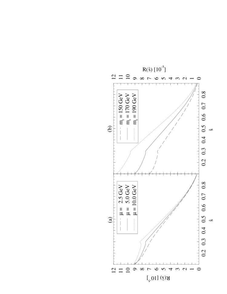
Figure 18: (a) $R(\hat{s})$ for $m_{\rm t}=170\,{\rm GeV}$, $\Lambda_{\overline{\rm MS}}^{(5)}=225\,{\rm MeV}$ and differents values of $\mu$. (b) $R(\hat{s})$ for $\mu=5\,{\rm GeV}$, $\Lambda_{\overline{\rm MS}}^{(5)}=225\,{\rm MeV}$ and various values of $m_{\rm t}$.

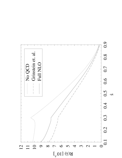
Figure 19: $R(\hat{s})$ for $m_{\rm t}=170\,{\rm GeV}$, $\Lambda_{\overline{\rm MS}}^{(5)}=225\,{\rm MeV}$ and $\mu=5\,{\rm GeV}$.

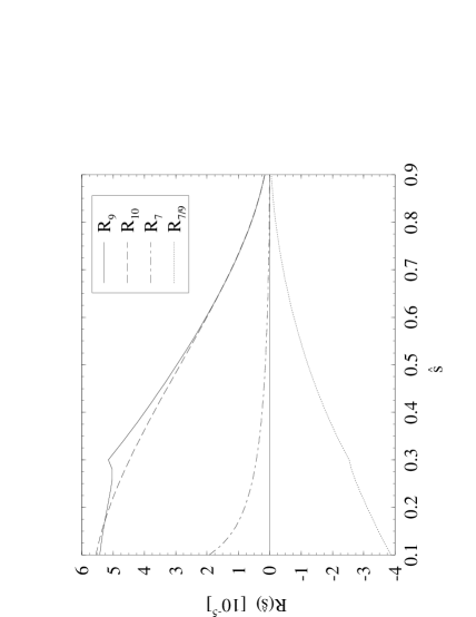
Figure 20: Comparison of the four different contributions to $R(\hat{s})$ according to eq. 6.64.

As seen in (6.64), $R(\hat{s})$ is governed by three coefficients, $\tilde{C}_{9}^{\rm eff}$, $\tilde{C}_{10}$ and $C_{7\gamma}^{(0){\rm eff}}$. The importance of various contributions is illustrated in fig. 20 [52], where $\Lambda_{\overline{\rm MS}}^{(5)}=225\,{\rm GeV}$, $m_{\rm t}=170\,{\rm GeV}$ and $\mu=5\,{\rm GeV}$ has been chosen. We show there $R(\hat{s})$ keeping only $\tilde{C}_{9}^{\rm eff}$, $\tilde{C}_{10}$, $C_{7\gamma}^{(0){\rm eff}}$ and the $C_{7\gamma}^{(0){\rm eff}}$–$\tilde{C}_{9}^{\rm eff}$ interference term, respectively. Denoting these contributions by $R_{9}$, $R_{10}$, $R_{7}$ and $R_{7/9}$ we observe that the term $R_{7}$ plays only a minor role in $R(\hat{s})$. On the other hand the presence of $C_{7\gamma}^{(0){\rm eff}}$ cannot be ignored because the interference term $R_{7/9}$ is significant. In fact the presence of this large interference term could be used to measure experimentally the relative sign of $C_{7\gamma}^{(0){\rm eff}}$ and $\mbox{Re}\,\tilde{C}_{9}^{\rm eff}$ [174, 175, 177, 180, 179], which with our conventions is negative in the Standard Model. However, the most important contributions are $R_{9}$ and $R_{10}$ in the full range of $\hat{s}$ considered. For $m_{\rm t}\approx 170\,{\rm GeV}$ these two contributions are roughly of the same size. Due to a strong $m_{\rm t}$ dependence of $R_{10}$, this contribution dominates for higher values of $m_{\rm t}$ and is less important than $R_{9}$ for $m_{\rm t}<170\,{\rm GeV}$. This behaviour is again similar to the one found in the case of $K_{\rm L}\to\pi^{0}e^{+}e^{-}$.

Finally varying the input parameters according to table 4 one finds for the non-resonant part of the branching ratio [190]

$$Br(B\to X_{s}\mu^{+}\mu^{-})_{\rm NR}=(5.7\pm 0.9)\cdot 10^{-6}$$ (6.74)

with a similar result in [172]. This should be compared with the most recent preliminary upper bound from D0 [191]:

$$Br(B\to X_{s}\mu^{+}\mu^{-})_{\rm NR}<3.6\cdot 10^{-5}$$ (6.75)

which improves the 1991 bound of UA1 [192] by roughly a factor of two. It is exciting that the experimental bound is only by a factor of five above the Standard Model expectations. D0 should be able to measure this branching ratio during the Run II at Tevatron.

One also finds [172]:

$$Br(B\to X_{s}e^{+}e^{-})_{\rm NR}=(8.4\pm 2.3)\cdot 10^{-6}$$ (6.76)

$$Br(B\to X_{s}\tau^{+}\tau^{-})_{\rm NR}=(2.6\pm 0.5)\cdot 10^{-6}$$ (6.77)

with similar results in [190].

6.4.5 Long Distance Contributions

The most recent discussions of the long-distance contributions to $B\to X_{s}l^{+}l^{-}$ can be found in [185]-[187] and in [172]. These contributions are due to the $J/\psi$ and $\psi^{\prime}$ resonances as well as $c\bar{c}$ continuum. They affect only the coefficient $\tilde{C}^{\rm eff}_{9}$. Clearly these contributions complicate the theoretical analysis. One possibility as done by experimentalists is to remove the resonance contributions from their final result in (6.75). Another possibility is to leave out in the integral over the lepton pair mass the regions dominated by $J/\psi$ and $\psi^{\prime}$: say $2.9\,{\rm GeV}-3.3\,{\rm GeV}$ and $3.6\,{\rm GeV}-3.8\,{\rm GeV}$, respectively. Finally one can include the resonances using phenomenological models. Details on all this can be found in the papers quoted above.

Another issue are the $1/m_{b}^{2}$ corrections. They have been first calculated in [193] with the result that they increase the entire dilepton mass spectrum by typically $10\%$. However, in this estimate the older values of the HQET parameters $\lambda_{1}$ and $\lambda_{2}$ have been used. In particular a positive value of $\lambda_{1}$ has been used. The use of the more recent negative values of $\lambda_{1}$ makes the corrections considerably smaller [172, 194]. Moreover the authors in [172] do not confirm the formulae in [193] and the net effect of $1/m^{2}_{b}$-corrections found in [172] is a suppression of $Br(B\to X_{s}l^{+}l^{-})$ by about $1.5\%$.

6.4.6 Other Distributions and Exclusive Decays

Clearly the calculation of $Br(B\to X_{s}\mu^{+}\mu^{-})$ and of the invariant dilepton mass spectrum is only a small part of the activities present in the literature in connection with this decay. The forward-backward charge asymmetry and various lepton polarization asymmetries (in particular in $B\to X_{s}\tau^{+}\tau^{-}$) should enable a detailed study of the dynamics of the Standard Model and the search for new physics beyond it [195, 95, 168, 196]. While the CP violation in $B\to X_{s}l^{+}l^{-}$ is strongly suppressed in the Standard Model [197], CP asymmetries of order $5\%$ are expected in $B\to X_{d}e^{+}e^{-}$ [198]. However, due to the expected branching ratio ${\cal O}(10^{-7})$ such an analysis is a formidable task.

The Standard Model predictions for exclusive channels $B_{d}\to K^{*}e^{+}e^{-}$ and $B_{d}\to K^{*}\mu^{+}\mu^{-}$ amount to $(2.3\pm 0.9)\cdot 10^{-6}$ and $(1.5\pm 0.6)\cdot 10^{-6}$, respectively [95]. This should be compared with the $90\%$ C.L. upper bounds $1.6\cdot 10^{-5}$ and $2.5\cdot 10^{-5}$ by CLEO [201] and CDF [200], respectively. Sensitivity of $3\cdot 10^{-7}$ should be reached for $B_{d}\to K^{*}\mu^{+}\mu^{-}$ by CDF during Run II. The exclusive channels, although not as clean as the inclusive ones, should also offer some insight in the dynamics involved [202].

6.4.7 Summary

The decays $B\to X_{s,d}l^{+}l^{-}$ remain to be an important arena for tests of the Standard Model and of its extensions. The discovery of the top quark, the calculations of NLO short distance QCD corrections and the estimate of $1/m_{b}^{2}$ corrections improved considerably the accuracy of the expected branching ratio and of various asymmetries and distributions.

Better estimates of long distance contributions, or equivalently efficient methods of their removal from the experimental data, are certainly desirable. It is exciting that the most recent D0 upper bound on $B\to X_{s}\mu^{+}\mu^{-}$ is only a factor of five away from the Standard Model expectations and that D0 as well as BABAR, BELLE, CLEO, CDF and HERA-B should be able to measure the branching ratio and the related distributions and asymmetries at the beginning of the next decade.

7 Rare $K$- and $B$-Decays

7.1 General Remarks

We will now move to discuss the semileptonic rare FCNC transitions $K^{+}\rightarrow\pi^{+}\nu\bar{\nu}$, $K_{\rm L}\to\pi^{0}\nu\bar{\nu}$, $B\to X_{s,d}\nu\bar{\nu}$, $B_{s,d}\to l^{+}l^{-}$ and $K_{\rm L}\to\mu^{+}\mu^{-}$. These decay modes are very similar in their structure which differs considerably from the one encountered in the decays $K\to\pi\pi$, $K\to\pi e^{+}e^{-}$, $B\to X_{s}\gamma$ and $B\to X_{s}\mu^{+}\mu^{-}$ discussed in previous sections. In particular:

• Within the Standard Model all the decays listed above are loop-induced semileptonic FCNC processes determined by $Z^{0}$-penguin and box diagrams (fig. 11 (d) and (e)).
  Thus, a distinguishing feature of the present class of decays is the absence of a photon penguin contribution. For the decay modes with neutrinos in the final state this is obvious, since the photon does not couple to neutrinos. For the mesons decaying into a charged lepton pair the photon penguin amplitude vanishes due to vector current conservation. Consequently the decays in question are governed by the functions $X_{0}(x_{t})$ and $Y_{0}(x_{t})$ (see (2.77) and (2.78)) which as seen in (2.83) and (2.84) exhibit strong $m_{\rm t}$ dependences.

• A particular and very important advantage of these decays is their clean theoretical character. This is related to the fact that the low energy hadronic matrix elements required are just the matrix elements of quark currents between hadron states, which can be extracted from the leading (non-rare) semileptonic decays. Other long-distance contributions (with the exception of the decay $K_{\rm L}\to\mu^{+}\mu^{-}$) are negligibly small. As a consequence of these features, the scale ambiguities, inherent to perturbative QCD, essentially constitute (except for $K_{\rm L}\to\mu^{+}\mu^{-}$) the only theoretical uncertainties present in the analysis of these decays. These theoretical uncertainties have been considerably reduced through the inclusion of the next-to-leading QCD corrections [46, 47, 48] as we will demonstrate below. The decay $K_{\rm L}\to\mu^{+}\mu^{-}$ receives important contributions from the two-photon intermediate state, which are difficult to calculate reliably. However, the short-distance part $(K_{\rm L}\to\mu^{+}\mu^{-})_{\rm SD}$ alone can be calculated reliably.

• The investigation of these low energy rare decay processes in conjunction with their theoretical cleanliness, allows to probe, albeit indirectly, high energy scales of the theory and in particular to measure the top quark couplings $V_{ts}$ and $V_{td}$. Moreover $K_{\rm L}\rightarrow\pi^{0}\nu\bar{\nu}$ offers a clean determination of the Wolfenstein parameter $\eta$ and as we will stress in section 11 offers the cleanest measurement of ${\rm Im}\lambda_{t}={\rm Im}V^{*}_{ts}V_{td}$ which governs all CP violating $K$-decays. However, the very fact that these processes are based on higher order electroweak effects implies that their branching ratios are expected to be very small and not easy to access experimentally.

	$K^{+}\rightarrow\pi^{+}\nu\bar{\nu}$	$K_{\rm L}\to\pi^{0}\nu\bar{\nu}$	$B\to X_{s}\nu\bar{\nu}$	$B\to X_{d}\nu\bar{\nu}$
	$(K_{\rm L}\to\mu^{+}\mu^{-})_{\rm SD}$		$B_{s}\to l^{+}l^{-}$	$B_{d}\to l^{+}l^{-}$
$\lambda_{c}$	$\sim\lambda$	(${\rm Im}\lambda_{c}\sim\lambda^{5}$)	$\sim\lambda^{2}$	$\sim\lambda^{3}$
$\lambda_{t}$	$\sim\lambda^{5}$	(${\rm Im}\lambda_{t}\sim\lambda^{5}$)	$\sim\lambda^{2}$	$\sim\lambda^{3}$

Table 18: Order of magnitude of CKM parameters relevant for the various decays, expressed in powers of the Wolfenstein parameter $\lambda=0.22$. In the case of $K_{\rm L}\to\pi^{0}\nu\bar{\nu}$, which is CP-violating, only the imaginary parts of $\lambda_{c,t}$ contribute.

The effective Hamiltonians governing the decays $K^{+}\rightarrow\pi^{+}\nu\bar{\nu}$, $(K_{\rm L}\to\mu^{+}\mu^{-})_{\rm SD}$, $K_{\rm L}\to\pi^{0}\nu\bar{\nu}$, $B\to X_{s,d}\nu\bar{\nu}$, $B\to l^{+}l^{-}$ resulting from the $Z^{0}$-penguin and box-type contributions can all be written in the following general form:

$${\cal H}_{\rm eff}={G_{\rm F}\over{\sqrt{2}}}{\alpha\over 2\pi\sin^{2}\Theta_{\rm W}}\left(\lambda_{c}F(x_{c})+\lambda_{t}F(x_{t})\right)(\bar{n}n^{\prime})_{V-A}(\bar{r}r)_{V-A}\,,$$ (7.1)

where $n$, $n^{\prime}$ denote down-type quarks ($n,n^{\prime}=d,s,b$ but $n\not=n^{\prime}$) and $r$ leptons, $r=l,\nu_{l}$ ($l=e,\mu,\tau$). The $\lambda_{i}$ are products of CKM elements, in the general case $\lambda_{i}=V^{*}_{in}V_{in^{\prime}}$. Furthermore $x_{i}=m^{2}_{i}/M^{2}_{W}$. The functions $F(x_{i})$ describe the dependence on the internal up-type quark masses $m_{i}$ (and on lepton masses if necessary) and are understood to include QCD corrections. They are increasing functions of the quark masses, a property that is particularly important for the top contribution. Since $F(x_{c})/F(x_{t})\approx{\cal O}(10^{-3})\ll 1$ the top contributions are by far dominant unless there is a partial compensation through the CKM factors $\lambda_{i}$. As seen in table 18 such a partial compensation takes place in $K^{+}\rightarrow\pi^{+}\nu\bar{\nu}$ and $(K_{\rm L}\to\mu^{+}\mu^{-})_{\rm SD}$ and consequently in these decays internal charm contributions, albeit smaller than the top contributions, have to be kept. On the other hand in the remaining decays the charm contributions can be safely neglected. Since the charm contributions involve QCD corrections with $\alpha_{s}(m_{c})$, the scale uncertainties in $K^{+}\rightarrow\pi^{+}\nu\bar{\nu}$ and $(K_{\rm L}\to\mu^{+}\mu^{-})_{\rm SD}$ are found to be larger than in the remaining decays in which the QCD effects enter only through $\alpha_{s}(m_{t})<\alpha_{s}(m_{c})$.

7.2 The Decay $K^{+}\rightarrow\pi^{+}\nu\bar{\nu}$

7.2.1 The effective Hamiltonian

The effective Hamiltonian for $K^{+}\rightarrow\pi^{+}\nu\bar{\nu}$ can be written as

$${\cal H}_{\rm eff}={G_{\rm F}\over{\sqrt{2}}}{\alpha\over 2\pi\sin^{2}\Theta_{\rm W}}\sum_{l=e,\mu,\tau}\left(V^{\ast}_{cs}V_{cd}X^{l}_{\rm NL}+V^{\ast}_{ts}V_{td}X(x_{t})\right)(\bar{s}d)_{V-A}(\bar{\nu}_{l}\nu_{l})_{V-A}\,.$$ (7.2)

The index $l$=$e$, $\mu$, $\tau$ denotes the lepton flavour. The dependence on the charged lepton mass resulting from the box-graph is negligible for the top contribution. In the charm sector this is the case only for the electron and the muon but not for the $\tau$-lepton.

The function $X(x)$ relevant for the top part is given by

$$X(x_{t})=X_{0}(x_{t})+\frac{\alpha_{s}}{4\pi}X_{1}(x_{t})$$ (7.3)

with the leading contribution $X_{0}(x)$ given in (2.77) and the QCD correction [47]

$$X_{1}(x)= - {23x+5x^{2}-4x^{3}\over 3(1-x)^{2}}+{x-11x^{2}+x^{3}+x^{4}\over(1-x)^{3}}\ln x$$ (7.4)

$$+ {8x+4x^{2}+x^{3}-x^{4}\over 2(1-x)^{3}}\ln^{2}x-{4x-x^{3}\over(1-x)^{2}}L_{2}(1-x)$$

$$+ 8x{\partial X_{0}(x)\over\partial x}\ln x_{\mu}\,,$$

where $x_{\mu}=\mu^{2}/M^{2}_{W}$ with $\mu=\mu_{t}={\cal O}(m_{t})$ and

$$L_{2}(1-x)=\int^{x}_{1}dt{\ln t\over 1-t}\,.$$ (7.5)

The $\mu$-dependence of the last term in (7.4) cancels to the considered order the $\mu$-dependence of the leading term $X_{0}(x(\mu))$. The leftover $\mu$-dependence in $X(x_{t})$ is tiny and will be given in connection with the discussion of the branching ratio below.

The function $X$ in (7.3) can also be written as

$$X(x)=\eta_{X}\cdot X_{0}(x),\qquad\quad\eta_{X}=0.985,$$ (7.6)

where $\eta_{X}$ summarizes the NLO corrections represented by the second term in (7.3). With $m_{\rm t}\equiv\overline{m}_{\rm t}(m_{\rm t})$ the QCD factor $\eta_{X}$ is practically independent of $m_{t}$ and $\Lambda_{\overline{MS}}$.

The expression corresponding to $X(x_{t})$ in the charm sector is the function $X^{l}_{\rm NL}$. It results from the NLO calculation [48] and is given explicitly in [48, 4]. The inclusion of NLO corrections reduced considerably the large $\mu_{c}$ dependence (with $\mu_{c}={\cal O}(m_{c})$) present in the leading order expressions for the charm contribution [203, 204, 205, 9]. Varying $\mu_{c}$ in the range $1\,{\rm GeV}\leq\mu_{c}\leq 3\,{\rm GeV}$ changes $X_{\rm NL}$ by roughly $24\%$ after the inclusion of NLO corrections to be compared with $56\%$ in the leading order. Further details can be found in [48, 4]. The impact of the $\mu_{c}$ uncertainties on the resulting branching ratio $Br(K^{+}\rightarrow\pi^{+}\nu\bar{\nu})$ is discussed below.

The numerical values for $X_{\rm NL}$ for $\mu=m_{\rm c}$ and several values of $\Lambda_{\overline{\rm MS}}^{(4)}$ and $m_{\rm c}(m_{\rm c})$ are given in table 19. The net effect of QCD corrections is to suppress the charm contribution by roughly $30\%$.

	$X^{e}_{\rm NL}/10^{-4}$			$X^{\tau}_{\rm NL}/10^{-4}$
$\Lambda_{\overline{\rm MS}}^{(4)}\ [\,{\rm MeV}]\;\backslash\;m_{\rm c}\ [\,{\rm GeV}]$	1.25	1.30	1.35	1.25	1.30	1.35
245	10.32	11.17	12.04	6.94	7.63	8.36
285	10.02	10.86	11.73	6.64	7.32	8.04
325	9.71	10.55	11.41	6.32	7.01	7.72
365	9.38	10.22	11.08	6.00	6.68	7.39
405	9.03	9.87	10.72	5.65	6.33	7.04

Table 19: The functions $X^{e}_{\rm NL}$ and $X^{\tau}_{\rm NL}$ for various $\Lambda_{\overline{\rm MS}}^{(4)}$ and $m_{\rm c}$.

7.2.2 Basic Phenomenology

We are now ready to present the expression for the branching fraction $Br(K^{+}\rightarrow\pi^{+}\nu\bar{\nu})$ and to collect various formulae relevant for phenomenological applications. Since the relevant hadronic matrix element of the weak current $(\bar{s}d)_{V-A}$ can be measured in the leading decay $K^{+}\to\pi^{0}e^{+}\nu$, the resulting theoretical expression for the branching fraction $Br(K^{+}\to\pi^{+}\nu\bar{\nu})$ can be related to the experimentally well known quantity $Br(K^{+}\to\pi^{0}e^{+}\nu)$ using isospin symmetry. Using the effective Hamiltonian (7.2) and summing over the three neutrino flavours one finds

$$Br(K^{+}\rightarrow\pi^{+}\nu\bar{\nu})=\kappa_{+}\cdot\left[\left({{\rm Im}\lambda_{t}\over\lambda^{5}}X(x_{t})\right)^{2}+\left({{\rm Re}\lambda_{c}\over\lambda}P_{0}(X)+{{\rm Re}\lambda_{t}\over\lambda^{5}}X(x_{t})\right)^{2}\right]$$ (7.7)

$$\kappa_{+}=r_{K^{+}}{3\alpha^{2}Br(K^{+}\to\pi^{0}e^{+}\nu)\over 2\pi^{2}\sin^{4}\Theta_{\rm W}}\lambda^{8}=4.11\cdot 10^{-11}\,,$$ (7.8)

where we have used

$$\alpha=\frac{1}{129},\qquad\sin^{2}\Theta_{\rm W}=0.23,\qquad Br(K^{+}\to\pi^{0}e^{+}\nu)=4.82\cdot 10^{-2}\,.$$ (7.9)

Here $\lambda_{i}=V^{\ast}_{is}V_{id}$ with $\lambda_{c}$ being real to a very high accuracy. $r_{K^{+}}=0.901$ summarizes isospin breaking corrections in relating $K^{+}\rightarrow\pi^{+}\nu\bar{\nu}$ to $K^{+}\to\pi^{0}e^{+}\nu$. These isospin breaking corrections are due to quark mass effects and electroweak radiative corrections and have been calculated in [206]. Next

$$P_{0}(X)=\frac{1}{\lambda^{4}}\left[\frac{2}{3}X^{e}_{\rm NL}+\frac{1}{3}X^{\tau}_{\rm NL}\right]$$ (7.10)

with the numerical values for $X_{\rm NL}^{l}$ given in table 19. The corresponding values for $P_{0}(X)$ as a function of $\Lambda_{\overline{MS}}$ and $m_{c}\equiv m_{c}(m_{c})$ are collected in table 20. We remark that a negligibly small term $\sim(X^{e}_{\rm NL}-X^{\tau}_{\rm NL})^{2}$ has been discarded in (7.7).

	$P_{0}(X)$
$\Lambda_{\overline{\rm MS}}^{(4)}$ $\backslash$ $m_{c}$	$1.25\,{\rm GeV}$	$1.30\,{\rm GeV}$	$1.35\,{\rm GeV}$
$245\,{\rm MeV}$	0.393	0.426	0.462
$285\,{\rm MeV}$	0.380	0.413	0.448
$325\,{\rm MeV}$	0.366	0.400	0.435
$365\,{\rm MeV}$	0.352	0.386	0.420
$405\,{\rm MeV}$	0.337	0.371	0.405

Table 20: The function $P_{0}(X)$ for various $\Lambda_{\overline{\rm MS}}^{(4)}$ and $m_{c}$.

Using the improved Wolfenstein parametrization and the approximate formulae (3.17) – (3.19) we can next put (7.7) into a more transparent form [63]:

$$Br(K^{+}\to\pi^{+}\nu\bar{\nu})=4.11\cdot 10^{-11}A^{4}X^{2}(x_{t})\frac{1}{\sigma}\left[(\sigma\bar{\eta})^{2}+\left(\varrho_{0}-\bar{\varrho}\right)^{2}\right]\,,$$ (7.11)

where

$$\sigma=\left(\frac{1}{1-\frac{\lambda^{2}}{2}}\right)^{2}\,.$$ (7.12)

The measured value of $Br(K^{+}\to\pi^{+}\nu\bar{\nu})$ then determines an ellipse in the $(\bar{\varrho},\bar{\eta})$ plane centered at $(\varrho_{0},0)$ with

$$\varrho_{0}=1+\frac{P_{0}(X)}{A^{2}X(x_{t})}$$ (7.13)

and having the squared axes

$$\bar{\varrho}_{1}^{2}=r^{2}_{0},\qquad\bar{\eta}_{1}^{2}=\left(\frac{r_{0}}{\sigma}\right)^{2}$$ (7.14)

where

$$r^{2}_{0}=\frac{1}{A^{4}X^{2}(x_{t})}\left[\frac{\sigma\cdot Br(K^{+}\to\pi^{+}\nu\bar{\nu})}{4.11\cdot 10^{-11}}\right]\,.$$ (7.15)

Note that $r_{0}$ depends only on the top contribution. The departure of $\varrho_{0}$ from unity measures the relative importance of the internal charm contributions.

The ellipse defined by $r_{0}$, $\varrho_{0}$ and $\sigma$ given above intersects with the circle (3.42). This allows to determine $\bar{\varrho}$ and $\bar{\eta}$ with

$$\bar{\varrho}=\frac{1}{1-\sigma^{2}}\left(\varrho_{0}-\sqrt{\sigma^{2}\varrho_{0}^{2}+(1-\sigma^{2})(r_{0}^{2}-\sigma^{2}R_{b}^{2})}\right),\qquad\bar{\eta}=\sqrt{R_{b}^{2}-\bar{\varrho}^{2}}$$ (7.16)

and consequently

$$R_{t}^{2}=1+R_{b}^{2}-2\bar{\varrho},$$ (7.17)

where $\bar{\eta}$ is assumed to be positive.

In the leading order of the Wolfenstein parametrization

$$\sigma\to 1,\qquad\bar{\eta}\to\eta,\qquad\bar{\varrho}\to\varrho$$ (7.18)

and $Br(K^{+}\to\pi^{+}\nu\bar{\nu})$ determines a circle in the $(\varrho,\eta)$ plane centered at $(\varrho_{0},0)$ and having the radius $r_{0}$ of (7.15) with $\sigma=1$. Formulae (7.16) and (7.17) then simplify to [48]

$$R_{t}^{2}=1+R_{b}^{2}+\frac{r_{0}^{2}-R_{b}^{2}}{\varrho_{0}}-\varrho_{0},\qquad\varrho=\frac{1}{2}\left(\varrho_{0}+\frac{R_{b}^{2}-r_{0}^{2}}{\varrho_{0}}\right).$$ (7.19)

Given $\bar{\varrho}$ and $\bar{\eta}$ one can determine $V_{td}$:

$$V_{td}=A\lambda^{3}(1-\bar{\varrho}-i\bar{\eta}),\qquad|V_{td}|=A\lambda^{3}R_{t}.$$ (7.20)

At this point a few remarks are in order:

• The long-distance contributions to $K^{+}\rightarrow\pi^{+}\nu\bar{\nu}$ have been studied in [207] and found to be very small: a few percent of the charm contribution to the amplitude at most, which is savely negligible.

• The determination of $|V_{td}|$ and of the unitarity triangle requires the knowledge of $V_{cb}$ (or $A$) and of $|V_{ub}/V_{cb}|$. Both values are subject to theoretical uncertainties present in the existing analyses of tree level decays. Whereas the dependence on $|V_{ub}/V_{cb}|$ is rather weak, the very strong dependence of $Br(K^{+}\rightarrow\pi^{+}\nu\bar{\nu})$ on $A$ or $V_{cb}$ makes a precise prediction for this branching ratio difficult at present. We will return to this below.

• The dependence of $Br(K^{+}\rightarrow\pi^{+}\nu\bar{\nu})$ on $m_{\rm t}$ is also strong. However $m_{\rm t}$ is known already within $\pm 4\%$ and consequently the related uncertainty in $Br(K^{+}\rightarrow\pi^{+}\nu\bar{\nu})$ is substantialy smaller than the corresponding uncertainty due to $V_{cb}$.

• Once $\varrho$ and $\eta$ are known precisely from CP asymmetries in $B$ decays, some of the uncertainties present in (7.11) related to $|V_{ub}/V_{cb}|$ (but not to $V_{cb}$) will be removed.

• A very clean determination of $\sin 2\beta$ without essentially any dependence on $m_{t}$ and $V_{cb}$ can be made by combining $Br(K^{+}\rightarrow\pi^{+}\nu\bar{\nu})$ with $Br(K_{\rm L}\rightarrow\pi^{0}\nu\bar{\nu})$ discussed below.

7.2.3 Numerical Analysis of $K^{+}\rightarrow\pi^{+}\nu\bar{\nu}$

Let us begin the numerical analysis by investigating the uncertainties in the prediction for $Br(K^{+}\rightarrow\pi^{+}\nu\bar{\nu})$ and in the determination of $|V_{td}|$ related to the choice of the renormalization scales $\mu_{t}$ and $\mu_{c}$ in the top part and the charm part, respectively. To this end we will fix the remaining parameters as follows:

$$m_{\rm c}\equiv\overline{m}_{\rm c}(m_{\rm c})=1.3\,{\rm GeV},\qquad m_{\rm t}\equiv\overline{m}_{\rm t}(m_{\rm t})=170\,{\rm GeV}$$ (7.21)

$$V_{cb}=0.040,\qquad|V_{ub}/V_{cb}|=0.08\,.$$ (7.22)

In the case of $Br(K^{+}\rightarrow\pi^{+}\nu\bar{\nu})$ we need the values of both $\bar{\varrho}$ and $\bar{\eta}$. Therefore in this case we will work with

$$\bar{\varrho}=0,\qquad\quad\bar{\eta}=0.36$$ (7.23)

rather than with $|V_{ub}/V_{cb}|$. Finally we will set $\Lambda_{\overline{MS}}^{(4)}=0.325\,{\rm GeV}$ and $\Lambda_{\overline{MS}}^{(5)}=0.225\,{\rm GeV}$ for the charm part and top part, respectively. We then vary the scales $\mu_{c}$ and $\mu_{t}$ entering $m_{c}(\mu_{c})$ and $m_{t}(\mu_{t})$, respectively, in the ranges

$$1\,{\rm GeV}\leq\mu_{c}\leq 3\,{\rm GeV},\qquad 100\,{\rm GeV}\leq\mu_{t}\leq 300\,{\rm GeV}\,.$$ (7.24)

The results of such an analysis are as follows [4]: The uncertainty in $Br(K^{+}\rightarrow\pi^{+}\nu\bar{\nu})$

$$0.68\cdot 10^{-10}\leq Br(K^{+}\rightarrow\pi^{+}\nu\bar{\nu})\leq 1.08\cdot 10^{-10}$$ (7.25)

present in the leading order is reduced to

$$0.79\cdot 10^{-10}\leq Br(K^{+}\rightarrow\pi^{+}\nu\bar{\nu})\leq 0.92\cdot 10^{-10}$$ (7.26)

after including NLO corrections. The difference in the numerics compared to [4] results from $r_{K^{+}}=1$ used there. Similarly one finds

$$8.24\cdot 10^{-3}\leq|V_{td}|\leq 10.97\cdot 10^{-3}\qquad{\rm LO}$$ (7.27)

$$9.23\cdot 10^{-3}\leq|V_{td}|\leq 10.10\cdot 10^{-3}\qquad{\rm NLO}\,,$$ (7.28)

where $Br(K^{+}\rightarrow\pi^{+}\nu\bar{\nu})=0.9\cdot 10^{-10}$ has been set. We observe that including the full next-to-leading corrections reduces the uncertainty in the determination of $|V_{td}|$ from $\pm 14\%$ (LO) to $\pm 4.6\%$ (NLO) in the present example. The main bulk of this theoretical error stems from the charm sector. Indeed, keeping $\mu_{c}=m_{c}$ fixed and varying only $\mu_{t}$, the uncertainties in the determination of $|V_{td}|$ would shrink to $\pm 4.7\%$ (LO) and $\pm 0.6\%$ (NLO). Similar comments apply to $Br(K^{+}\rightarrow\pi^{+}\nu\bar{\nu})$ where, as seen in (7.25) and (7.26), the theoretical uncertainty due to $\mu_{c,t}$ is reduced from $\pm 22\%$ (LO) to $\pm 7\%$ (NLO).

Finally using the input parameters of table 4 and performing two types of error analysis one finds [94]

$$Br(K^{+}\rightarrow\pi^{+}\nu\bar{\nu})=\left\{\begin{array}[]{ll}(9.1\pm 3.2)\cdot 10^{-11}&{\rm Scanning}\\ (8.0\pm 1.5)\cdot 10^{-11}&{\rm Gaussian}\,,\end{array}\right.$$ (7.29)

where the error comes dominantly from the uncertainties in the CKM parameters.

7.2.4 Summary and Outlook

The accuracy of the Standard Model prediction for $Br(K^{+}\rightarrow\pi^{+}\nu\bar{\nu})$ has improved considerably during the last five years. Indeed in the Top Quark Story [3] a range $(5-80)\cdot 10^{-11}$ can still be found. This progress can be traced back to the improved values of $m_{\rm t}$ and $|V_{cb}|$ and to the inclusion of NLO QCD corrections which considerably reduced the scale uncertainties in the charm sector. It is expected [4] that further progress in the determination of CKM parameters via the standard analysis of section 4.6 could reduce the errors in (7.29) by at least a factor of two during the next five years.

The present experimental bound on $Br(K^{+}\to\pi^{+}\nu\bar{\nu})$ is [208]:

$$Br(K^{+}\rightarrow\pi^{+}\nu\bar{\nu})<2.4\cdot 10^{-9}\,.$$ (7.30)

This is about a factor of 25 above the Standard Model expectations (7.29). A new bound $2\cdot 10^{-10}$ for this decay is expected from E787 at AGS in Brookhaven in 1997. In view of the clean character of this decay a measurement of its branching ratio at this level would signal the presence of physics beyond the Standard Model. The Standard Model sensitivity is expected to be reached at AGS around the year 2000 [209]. Recently also an experiment has been proposed to measure $K^{+}\rightarrow\pi^{+}\nu\bar{\nu}$ at the Fermilab Main Injector [210].

7.3 The Decay $K_{\rm L}\to\pi^{0}\nu\bar{\nu}$

7.3.1 The effective Hamiltonian

The effective Hamiltonian for $K_{\rm L}\to\pi^{0}\nu\bar{\nu}$ is given as follows:

$${\cal H}_{\rm eff}={G_{\rm F}\over\sqrt{2}}{\alpha\over 2\pi\sin^{2}\Theta_{\rm W}}V^{\ast}_{ts}V_{td}X(x_{t})(\bar{s}d)_{V-A}(\bar{\nu}\nu)_{V-A}+h.c.\,,$$ (7.31)

where the function $X(x_{t})$, present already in $K^{+}\rightarrow\pi^{+}\nu\bar{\nu}$, includes NLO corrections and is given in (7.3).

Since $K_{\rm L}\rightarrow\pi^{0}\nu\bar{\nu}$ proceeds in the Standard Model almost entirely through CP violation [211], it is completely dominated by short-distance loop diagrams with top quark exchanges. The charm contribution, as we discussed above, can be fully neglected and the theoretical uncertainties present in $K^{+}\rightarrow\pi^{+}\nu\bar{\nu}$ due to $m_{c}$, $\mu_{c}$ and $\Lambda_{\overline{MS}}$ are absent here. Consequently the rare decay $K_{\rm L}\rightarrow\pi^{0}\nu\bar{\nu}$ is even cleaner than $K^{+}\rightarrow\pi^{+}\nu\bar{\nu}$ and is very well suited for the determination of the Wolfenstein parameter $\eta$ and ${\rm Im}\lambda_{t}$.

Before going into the details it is appropriate to clarify one point [212, 213]. It is usually stated in the literature that the decay $K_{\rm L}\rightarrow\pi^{0}\nu\bar{\nu}$ is dominated by direct CP violation. Now the standard definition of the direct CP violation (see section 8 and e.g. (8.127)) requires the presence of strong phases which are completely neglegible in $K_{\rm L}\rightarrow\pi^{0}\nu\bar{\nu}$. Consequently the violation of CP symmetry in $K_{\rm L}\rightarrow\pi^{0}\nu\bar{\nu}$ arises through the interference between $K^{0}-\bar{K}^{0}$ mixing and the decay amplitude. This type of CP violation is often called mixing-induced CP violation. However, as already pointed out by Littenberg [211], the contribution of CP violation to $K_{\rm L}\rightarrow\pi^{0}\nu\bar{\nu}$ via $K^{0}-\bar{K}^{0}$ mixing alone is tiny. It gives $Br(K_{\rm L}\rightarrow\pi^{0}\nu\bar{\nu})\approx 5\cdot 10^{-15}$. Consequently, in this sence, CP violation in $K_{\rm L}\rightarrow\pi^{0}\nu\bar{\nu}$ with $Br(K_{\rm L}\rightarrow\pi^{0}\nu\bar{\nu})={\cal O}(10^{-11})$ is a manifestation of CP violation in the decay and as such deserves the name of direct CP violation. In other words the difference in the magnitude of CP violation in $K_{\rm L}\to\pi\pi~{}(\varepsilon_{K})$ and $K_{\rm L}\rightarrow\pi^{0}\nu\bar{\nu}$ is a signal of direct CP violation and measuring $K_{\rm L}\rightarrow\pi^{0}\nu\bar{\nu}$ at the expected level would rule out superweak scenarios. More details on this issue can be found in [212, 213, 215].

7.3.2 Master Formulae for $Br(K_{\rm L}\rightarrow\pi^{0}\nu\bar{\nu})$

Using the effective Hamiltonian (7.31) and summing over three neutrino flavours one finds

$$Br(K_{\rm L}\to\pi^{0}\nu\bar{\nu})=\kappa_{\rm L}\cdot\left({{\rm Im}\lambda_{t}\over\lambda^{5}}X(x_{t})\right)^{2}$$ (7.32)

$$\kappa_{\rm L}=\frac{r_{K_{\rm L}}}{r_{K^{+}}}{\tau(K_{\rm L})\over\tau(K^{+})}\kappa_{+}=1.80\cdot 10^{-10}$$ (7.33)

with $\kappa_{+}$ given in (7.8) and $r_{K_{\rm L}}=0.944$ summarizing isospin breaking corrections in relating $K_{\rm L}\rightarrow\pi^{0}\nu\bar{\nu}$ to $K^{+}\to\pi^{0}e^{+}\nu$ [206].

Using the Wolfenstein parametrization we can rewrite (7.32) as

$$Br(K_{\rm L}\rightarrow\pi^{0}\nu\bar{\nu})=1.80\cdot 10^{-10}\eta^{2}A^{4}X^{2}(x_{t})$$ (7.34)

or

$$Br(K_{\rm L}\rightarrow\pi^{0}\nu\bar{\nu})=3.29\cdot 10^{-5}\eta^{2}|V_{cb}|^{4}X^{2}(x_{t})$$ (7.35)

or using

$$X(x_{t})=0.65\cdot x_{t}^{0.575}$$ (7.36)

$$Br(K_{\rm L}\to\pi^{0}\nu\bar{\nu})=3.0\cdot 10^{-11}\left[\frac{\eta}{0.39}\right]^{2}\left[\frac{\overline{m}_{\rm t}(m_{\rm t})}{170~{}GeV}\right]^{2.3}\left[\frac{\mid V_{cb}\mid}{0.040}\right]^{4}\,.$$ (7.37)

A few remarks are in order:

• The determination of $\eta$ using $Br(K_{\rm L}\rightarrow\pi^{0}\nu\bar{\nu})$ requires the knowledge of $V_{cb}$ and $m_{t}$. The very strong dependence on $V_{cb}$ or $A$ makes a precise prediction for this branching ratio difficult at present.

• It was pointed out in [214] that the strong dependence of $Br(K_{\rm L}\rightarrow\pi^{0}\nu\bar{\nu})$ on $V_{cb}$, together with the clean nature of this decay, can be used to determine this element without any hadronic uncertainties. To this end $\eta$ and $m_{t}$ have to be known with sufficient precision in addition to $Br(K_{\rm L}\rightarrow\pi^{0}\nu\bar{\nu})$. Inverting (7.37) one finds

  $$|V_{cb}|=40.0\cdot 10^{-3}\sqrt{\frac{0.39}{\eta}}\left[\frac{170\,{\rm GeV}}{\overline{m}_{\rm t}(m_{\rm t})}\right]^{0.575}\left[\frac{Br(K_{\rm L}\rightarrow\pi^{0}\nu\bar{\nu})}{3\cdot 10^{-11}}\right]^{1/4}\,.$$ (7.38)

  We note that the weak dependence of $V_{cb}$ on $Br(K_{\rm L}\rightarrow\pi^{0}\nu\bar{\nu})$ allows to achieve a high precision for this CKM element even when $Br(K_{\rm L}\rightarrow\pi^{0}\nu\bar{\nu})$ is known with only relatively moderate accuracy, e.g. 10–15%. A numerical analysis of (7.38) can be found in [214, 215] and will be presented in section 11.

7.3.3 Numerical Analysis of $K_{\rm L}\rightarrow\pi^{0}\nu\bar{\nu}$

The $\mu_{t}$-uncertainties present in the function $X(x_{t})$ have already been discussed in connection with $K^{+}\rightarrow\pi^{+}\nu\bar{\nu}$. After the inclusion of NLO corrections they are so small that they can be neglected for all practical purposes. At the level of $Br(K_{\rm L}\rightarrow\pi^{0}\nu\bar{\nu})$ the ambiguity in the choice of $\mu_{t}$ is reduced from $\pm 10\%$ (LO) down to $\pm 1\%$ (NLO), which considerably increases the predictive power of the theory. Varying $\mu_{t}$ according to (7.24) and using the input parameters as in the case of $K^{+}\rightarrow\pi^{+}\nu\bar{\nu}$ we find that the uncertainty in $Br(K_{\rm L}\rightarrow\pi^{0}\nu\bar{\nu})$

$$2.53\cdot 10^{-11}\leq Br(K_{\rm L}\rightarrow\pi^{0}\nu\bar{\nu})\leq 3.08\cdot 10^{-11}$$ (7.39)

present in the leading order is reduced to

$$2.64\cdot 10^{-11}\leq Br(K_{\rm L}\rightarrow\pi^{0}\nu\bar{\nu})\leq 2.72\cdot 10^{-11}$$ (7.40)

after including NLO corrections. This means that the theoretical uncertainty in the determination of $\eta$ amounts to only $\pm 0.7\%$ which is safely negligible.

Using the input parameters of table 4 one finds [94]

$$Br(K_{\rm L}\rightarrow\pi^{0}\nu\bar{\nu})=\left\{\begin{array}[]{ll}(2.8\pm 1.7)\cdot 10^{-11}&{\rm Scanning}\\ (2.6\pm 0.9)\cdot 10^{-11}&{\rm Gaussian}\end{array}\right.$$ (7.41)

where the error comes dominantly from the uncertainties in the CKM parameters.

7.3.4 Summary and Outlook

The accuracy of the Standard Model prediction for $Br(K_{\rm L}\rightarrow\pi^{0}\nu\bar{\nu})$ has improved considerably during the last five years. Indeed in the Top Quark Story [3] values as high as $15\cdot 10^{-11}$ can be found. This progress can be traced back mainly to the improved values of $m_{\rm t}$ and $|V_{cb}|$ and to some extent to the inclusion of NLO QCD corrections. It is expected [4] that further progress in the determination of CKM parameters via the standard analysis of section 4 could reduce the errors in (7.41) by at least a factor of two during the next five years.

The present upper bound on $Br(K_{\rm L}\to\pi^{0}\nu\bar{\nu})$ from FNAL experiment E731 [216] is

$$Br(K_{\rm L}\rightarrow\pi^{0}\nu\bar{\nu})<5.8\cdot 10^{-5}\,.$$ (7.42)

This is about six orders of magnitude above the Standard Model expectation (7.41).

How large could $Br(K_{\rm L}\rightarrow\pi^{0}\nu\bar{\nu})$ really be? As shown recently in [212] one can easily derive by means of isospin symmetry the following model independent bound:

$$Br(K_{\rm L}\rightarrow\pi^{0}\nu\bar{\nu})<4.4\cdot Br(K^{+}\rightarrow\pi^{+}\nu\bar{\nu})$$ (7.43)

which through (7.30) gives

$$Br(K_{\rm L}\rightarrow\pi^{0}\nu\bar{\nu})<1.1\cdot 10^{-8}$$ (7.44)

This bound is much stronger than the direct experimental bound in (7.42). With the upper bound $Br(K^{+}\rightarrow\pi^{+}\nu\bar{\nu})<2\cdot 10^{-10}$ expected this year from BNL, the bound in (7.44) can be improved to $9\cdot 10^{-10}$.

Now FNAL-E799 expects to reach the accuracy ${\cal O}(10^{-8})$ and a very interesting new experiment at Brookhaven (BNL E926) [209] expects to reach the single event sensitivity $2\cdot 10^{-12}$ allowing a $10\%$ measurement of the expected branching ratio. There are furthermore plans to measure this gold-plated decay with comparable sensitivity at Fermilab [217] and KEK [218].

Figure 21: Unitarity triangle from $K\to\pi\nu\bar{\nu}$.

7.4 Unitarity Triangle and $\sin 2\beta$ from $K\to\pi\nu\bar{\nu}$

The measurement of $Br(K^{+}\rightarrow\pi^{+}\nu\bar{\nu})$ and $Br(K_{\rm L}\rightarrow\pi^{0}\nu\bar{\nu})$ can determine the unitarity triangle completely, (see fig. 21), provided $m_{\rm t}$ and $V_{cb}$ are known [3]. Using these two branching ratios simultaneously allows to eliminate $|V_{ub}/V_{cb}|$ from the analysis which removes a considerable uncertainty. Indeed it is evident from (7.7) and (7.32) that, given $Br(K^{+}\rightarrow\pi^{+}\nu\bar{\nu})$ and $Br(K_{\rm L}\rightarrow\pi^{0}\nu\bar{\nu})$, one can extract both ${\rm Im}\lambda_{t}$ and ${\rm Re}\lambda_{t}$. One finds [219, 4]

$${\rm Im}\lambda_{t}=\lambda^{5}{\sqrt{B_{2}}\over X(x_{t})}\qquad{\rm Re}\lambda_{t}=-\lambda^{5}{{{\rm Re}\lambda_{c}\over\lambda}P_{0}(X)+\sqrt{B_{1}-B_{2}}\over X(x_{t})}\,,$$ (7.45)

where we have defined the “reduced” branching ratios

$$B_{1}={Br(K^{+}\rightarrow\pi^{+}\nu\bar{\nu})\over 4.11\cdot 10^{-11}}\qquad B_{2}={Br(K_{\rm L}\rightarrow\pi^{0}\nu\bar{\nu})\over 1.80\cdot 10^{-10}}\,.$$ (7.46)

Using next the expressions for ${\rm Im}\lambda_{t}$, ${\rm Re}\lambda_{t}$ and ${\rm Re}\lambda_{c}$ given in (3.17) – (3.19) we find

$$\bar{\varrho}=1+{P_{0}(X)-\sqrt{\sigma(B_{1}-B_{2})}\over A^{2}X(x_{t})}\,,\qquad\bar{\eta}={\sqrt{B_{2}}\over\sqrt{\sigma}A^{2}X(x_{t})}$$ (7.47)

with $\sigma$ defined in (7.12). An exact treatment of the CKM matrix shows that the formulae (7.47) are rather precise [219]. The error in $\bar{\eta}$ is below 0.1% and $\bar{\varrho}$ may deviate from the exact expression by at most $\Delta\bar{\varrho}=0.02$ with essentially negligible error for $0\leq\bar{\varrho}\leq 0.25$.

Using (7.47) one finds subsequently [219]

$$r_{s}=r_{s}(B_{1},B_{2})\equiv{1-\bar{\varrho}\over\bar{\eta}}=\cot\beta\,,\qquad\sin 2\beta=\frac{2r_{s}}{1+r^{2}_{s}}$$ (7.48)

with

$$r_{s}(B_{1},B_{2})=\sqrt{\sigma}{\sqrt{\sigma(B_{1}-B_{2})}-P_{0}(X)\over\sqrt{B_{2}}}\,.$$ (7.49)

Thus within the approximation of (7.47) $\sin 2\beta$ is independent of $V_{cb}$ (or $A$) and $m_{t}$. An exact treatment of the CKM matrix confirms this finding to a high accuracy. The dependence on $V_{cb}$ and $m_{t}$ enters only at order ${\cal O}(\lambda^{2})$ and as a numerical analysis shows this dependence can be fully neglected.

It should be stressed that $\sin 2\beta$ determined this way depends only on two measurable branching ratios and on the function $P_{0}(X)$ which is completely calculable in perturbation theory. Consequently this determination is free from any hadronic uncertainties and its accuracy can be estimated with a high degree of confidence.

An extensive numerical analysis of the formulae above has been presented in [219, 215]. We summarize the results of the latter paper. Assuming that the branching ratios are known to within $\pm 10\%$

$$Br(K^{+}\rightarrow\pi^{+}\nu\bar{\nu})=(1.0\pm 0.1)\cdot 10^{-10}\,,\qquad Br(K_{\rm L}\rightarrow\pi^{0}\nu\bar{\nu})=(3.0\pm 0.30)\cdot 10^{-11}$$ (7.50)

and choosing

$$m_{t}=(170\pm 3)\,{\rm GeV},\quad P_{0}(X)=0.40\pm 0.06,\quad|V_{cb}|=0.040\pm 0.002$$ (7.51)

one finds the results given in the second column of table 21. In the third coulumn the results for the choice $|V_{cb}|=0.040\pm 0.001$ are shown. It should be remarked that the quoted errors for the input parameter are quite reasonable if one keeps in mind that it will take five years to achieve the accuracy assumed in (7.50). The error in $P_{0}(X)$ in (7.51) results from the errors (see table 20 and (7.24)) in $\Lambda_{\overline{\rm MS}}^{(4)}$, $m_{c}$ and $\mu_{c}$ added quadratically. Doubling the error in $m_{c}$ would give $P_{0}(X)=0.40\pm 0.09$ and an increase of the errors in $|V_{td}|/10^{-3}$, $\bar{\varrho}$ and $\sin 2\beta$ by at most $\pm 0.2$, $\pm 0.02$ and $\pm 0.01$ respectively, without any changes in $\bar{\eta}$ and ${\rm Im}\lambda_{t}$.

	$|V_{cb}|=0.040\pm 0.002$	$|V_{cb}|=0.040\pm 0.001$.
$|V_{td}|/10^{-3}$	$10.3\pm 1.1$	$10.3\pm 0.9$
$|V_{ub}/V_{cb}|$	$0.089\pm 0.017$	$0.089\pm 0.011$
$\bar{\varrho}$	$-0.10\pm 0.16$	$-0.10\pm 0.12$
$\bar{\eta}$	$0.38\pm 0.04$	$0.38\pm 0.03$
$\sin 2\beta$	$0.62\pm 0.05$	$0.62\pm 0.05$
${\rm Im}\lambda_{t}/10^{-4}$	$1.37\pm 0.07$	$1.37\pm 0.07$

Table 21: Illustrative example of the determination of CKM parameters from $K\to\pi\nu\bar{\nu}$ for two choices of $V_{cb}$ and other parameters given in the text.

We observe that respectable determinations of all considered quantities except for $\bar{\varrho}$ can be obtained. Of particular interest are the accurate determinations of $\sin 2\beta$ and of ${\rm Im}\lambda_{t}$. The latter quantity as seen in (7.45) can be obtained from $K_{\rm L}\to\pi^{0}\nu\bar{\nu}$ alone and does not require knowledge of $V_{cb}$.

As pointed out in [215] and discussed in section 11, $K_{\rm L}\to\pi^{0}\nu\bar{\nu}$ appears to be the best decay to measure ${\rm Im}\lambda_{t}$; even better than the CP asymmetries in $B$ decays discussed in the following sections. The importance of measuring accurately ${\rm Im}\lambda_{t}$ is evident. It plays a central role in the phenomenology of CP violation in $K$ decays and is furthermore equivalent to the Jarlskog parameter $J_{\rm CP}$ [220], the invariant measure of CP violation in the Standard Model, $J_{\rm CP}=\lambda(1-\lambda^{2}/2){\rm Im}\lambda_{t}$.

The accuracy to which $\sin 2\beta$ can be obtained from $K\to\pi\nu\bar{\nu}$ is, in the example discussed above, comparable to the one expected in determining $\sin 2\beta$ from CP asymmetries in $B$ decays prior to LHC experiments. In this case $\sin 2\beta$ is determined best by measuring CP violation in $B_{d}\to J/\psi K_{\rm S}$ as we will discuss in detail in the following sections. Using the formula (8.59) for the corresponding time-integrated CP asymmetry one finds an interesting connection between rare $K$ decays and $B$ physics [219]

$${2r_{s}(B_{1},B_{2})\over 1+r^{2}_{s}(B_{1},B_{2})}=-a_{\mbox{{\scriptsize CP}}}(B_{d}\to J/\psi K_{\mbox{{\scriptsize S}}}){1+x^{2}_{d}\over x_{d}}$$ (7.52)

which must be satisfied in the Standard Model. We stress that except for $P_{0}(X)$ given in table 20 all quantities in (7.52) can be directly measured in experiment and that this relationship is essentially independent of $m_{t}$ and $V_{cb}$. Due to very small theoretical uncertainties in (7.52), this relation is particularly suited for tests of CP violation in the Standard Model and offers a powerful tool to probe the physics beyond it. Further comparision between the potential of $K\to\pi\nu\bar{\nu}$ and CP asymmetries in $B$ decays will be given in section 11.

7.5 The Decays $B\to X_{s,d}\nu\bar{\nu}$

7.5.1 Effective Hamiltonian

The decays $B\to X_{s,d}\nu\bar{\nu}$ are the theoretically cleanest decays in the field of rare $B$-decays. They are dominated by the same $Z^{0}$-penguin and box diagrams involving top quark exchanges which we encountered already in the case of $K^{+}\rightarrow\pi^{+}\nu\bar{\nu}$ and $K_{\rm L}\rightarrow\pi^{0}\nu\bar{\nu}$ except for the appropriate change of the external quark flavours. Since the change of external quark flavours has no impact on the $m_{t}$ dependence, the latter is fully described by the function $X(x_{t})$ in (7.3) which includes the NLO corrections [47]. The charm contribution as discussed at the beginning of this section is fully neglegible here and the resulting effective Hamiltonian is very similar to the one for $K_{\rm L}\rightarrow\pi^{0}\nu\bar{\nu}$ given in (7.31). For the decay $B\to X_{s}\nu\bar{\nu}$ it reads

$${\cal H}_{\rm eff}={G_{\rm F}\over\sqrt{2}}{\alpha\over 2\pi\sin^{2}\Theta_{\rm W}}V^{\ast}_{tb}V_{ts}X(x_{t})(\bar{b}s)_{V-A}(\bar{\nu}\nu)_{V-A}+h.c.$$ (7.53)

with $s$ replaced by $d$ in the case of $B\to X_{d}\nu\bar{\nu}$.

The theoretical uncertainties related to the renormalization scale dependence are as in $K_{\rm L}\rightarrow\pi^{0}\nu\bar{\nu}$ and can be essentially neglected. On the other hand $B\to X_{s,d}\nu\bar{\nu}$ are CP conserving and consequently the relevant branching ratios are sensitive to $|V_{td}|$ and $|V_{ts}|$ as opposed to $Br(K_{\rm L}\rightarrow\pi^{0}\nu\bar{\nu})$ in which ${\rm Im}(V^{\ast}_{ts}V_{td})$ enters. As we will stress below the measurement of both $B\to X_{s}\nu\bar{\nu}$ and $B\to X_{d}\nu\bar{\nu}$ offers the cleanest determination of the ratio $|V_{td}|/|V_{ts}|$.

7.5.2 The Branching Ratios

The calculation of the branching fractions for $B\to X_{s,d}\nu\bar{\nu}$ can be done similarly to $B\to X_{s}\gamma$ and $B\to X_{s}\mu^{+}\mu^{-}$ in the spectator model corrected for short distance QCD effects. Normalizing as in these latter decays to $Br(B\to X_{c}e\bar{\nu})$ and summing over three neutrino flavours one finds

$$\frac{Br(B\to X_{s}\nu\bar{\nu})}{Br(B\to X_{c}e\bar{\nu})}=\frac{3\alpha^{2}}{4\pi^{2}\sin^{4}\Theta_{\rm W}}\frac{|V_{ts}|^{2}}{|V_{cb}|^{2}}\frac{X^{2}(x_{t})}{f(z)}\frac{\bar{\eta}}{\kappa(z)}\,.$$ (7.54)

Here $f(z)$ is the phase-space factor for $B\to X_{c}e\bar{\nu}$ defined already in (6.25) and $\kappa(z)$ is the corresponding QCD correction given in (6.40). The factor $\bar{\eta}$ represents the QCD correction to the matrix element of the $b\to s\nu\bar{\nu}$ transition due to virtual and bremsstrahlung contributions and is given by the well known expression

$$\bar{\eta}=\kappa(0)=1+\frac{2\alpha_{s}(m_{b})}{3\pi}\left(\frac{25}{4}-\pi^{2}\right)\approx 0.83\,.$$ (7.55)

In the case of $B\to X_{d}\nu\bar{\nu}$ one has to replace $V_{ts}$ by $V_{td}$ which results in a decrease of the branching ratio by roughly an order of magnitude.

It should be noted that $Br(B\to X_{s}\nu\bar{\nu})$ as given in (7.54) is in view of $|V_{ts}/V_{cb}|^{2}\approx 0.95\pm 0.03$ essentially independent of the CKM parameters and the main uncertainty resides in the value of $m_{\rm t}$ which is already rather precisely known. Setting $Br(B\to X_{c}e\bar{\nu})=10.4\%$, $f(z)=0.54$, $\kappa(z)=0.88$ and using the values in (7.9) we have

$$Br(B\to X_{s}\nu\bar{\nu})=3.7\cdot 10^{-5}\,\frac{|V_{ts}|^{2}}{|V_{cb}|^{2}}\,\left[\frac{\overline{m}_{\rm t}(m_{\rm t})}{170\,{\rm GeV}}\right]^{2.30}\,.$$ (7.56)

Taking next, in accordance with (6.42), $\kappa(z)=0.88$, $f(z)=0.54\pm 0.04$ and $Br(B\to X_{c}e\bar{\nu})=(10.4\pm 0.4)\%$ and using the input parameters of table 4 one finds [94]

$$Br(B\to X_{s}\nu\bar{\nu})=\left\{\begin{array}[]{ll}(3.4\pm 0.7)\cdot 10^{-5}&{\rm Scanning}\\ (3.2\pm 0.4)\cdot 10^{-5}&{\rm Gaussian}\,.\end{array}\right.$$ (7.57)

These values are by $10\%$ lower than the ones given in [4] where $f(z)=0.49$ has been used.

What about the data? One of the high-lights of FCNC-1996 was the upper bound:

$$Br(B\to X_{s}\nu\bar{\nu})<7.7\cdot 10^{-4}\quad(90\%\,\,\mbox{C.L.})$$ (7.58)

obtained for the first time by ALEPH [221]. This is only a factor of 20 above the Standard Model expectation. Even if the actual measurement of this decay is extremly difficult, all efforts should be made to measure it. One should also make attempts to measure $Br(B\to X_{d}\nu\bar{\nu})$. Indeed

$$\frac{Br(B\to X_{d}\nu\bar{\nu})}{Br(B\to X_{s}\nu\bar{\nu})}=\frac{|V_{td}|^{2}}{|V_{ts}|^{2}}$$ (7.59)

offers the cleanest direct determination of $|V_{td}|/|V_{ts}|$ as all uncertainties related to $m_{\rm t}$, $f(z)$ and $Br(B\to X_{c}e\bar{\nu})$ cancel out.

Meanwhile the bound in (7.58) puts some constraints on exotic physics beyond the Standard Model [223]. Finally, we would like to mention the new $90\%$ C.L. bounds for the exclusive channels: $Br(B_{d}\to K^{*}\nu\bar{\nu})<1\cdot 10^{-3}$ and $Br(B_{s}\to\phi\nu\bar{\nu})<5.4\cdot 10^{-3}$ from DELPHI [222] which should be compared with ${\cal O}(10^{-5})$ in the Standard Model. As usual the exclusive channels are subject to hadronic uncertainties.

7.6 The Decays $B_{s,d}\to l^{+}l^{-}$

7.6.1 The Effective Hamiltonian

The decays $B_{s,d}\to l^{+}l^{-}$ are after $B\to X_{s,d}\nu\bar{\nu}$ the theoretically cleanest decays in the field of rare $B$-decays. They are dominated by the $Z^{0}$-penguin and box diagrams involving top quark exchanges which we encountered already in the case of $B\to X_{s,d}\nu\bar{\nu}$ except that due to charged leptons in the final state the charge flow in the internal lepton line present in the box diagram is reversed. This results in a different $m_{\rm t}$ dependence summarized by the function $Y(x_{t})$, the NLO generalization [47] of the function $Y_{0}(x_{t})$ given in (2.78). The charm contributions as discussed at the beginning of this section are fully negligible here and the resulting effective Hamiltonian is given for $B_{s}\to l^{+}l^{-}$ as follows:

$${\cal H}_{\rm eff}=-{G_{\rm F}\over\sqrt{2}}{\alpha\over 2\pi\sin^{2}\Theta_{\rm W}}V^{\ast}_{tb}V_{ts}Y(x_{t})(\bar{b}s)_{V-A}(\bar{l}l)_{V-A}+h.c.$$ (7.60)

with $s$ replaced by $d$ in the case of $B_{d}\to l^{+}l^{-}$.

The function $Y(x)$ is given by

$$Y(x_{t})=Y_{0}(x_{t})+\frac{\alpha_{s}}{4\pi}Y_{1}(x_{t})\,,$$ (7.61)

where $Y_{0}(x_{t})$ can be found in (2.78) and [47]

$$Y_{1}(x)= {4x+16x^{2}+4x^{3}\over 3(1-x)^{2}}-{4x-10x^{2}-x^{3}-x^{4}\over(1-x)^{3}}\ln x$$ (7.62)

$$+ {2x-14x^{2}+x^{3}-x^{4}\over 2(1-x)^{3}}\ln^{2}x+{2x+x^{3}\over(1-x)^{2}}L_{2}(1-x)$$

$$+ 8x{\partial Y_{0}(x)\over\partial x}\ln x_{\mu}\,.$$

The $\mu$-dependence of the last term in (7.62) cancels to the considered order the one of the leading term $Y_{0}(x(\mu))$. The leftover $\mu$-dependence in $Y(x_{t})$ is tiny and amounts to an uncertainty of $\pm 1\%$ at the level of the branching ratio.

The function $Y(x)$ of (7.61) can also be written as

$$Y(x)=\eta_{Y}\cdot Y_{0}(x)\,,\qquad\quad\eta_{Y}=1.026\pm 0.006\,,$$ (7.63)

where $\eta_{Y}$ summarizes the NLO corrections. With $m_{\rm t}\equiv\overline{m}_{\rm t}(m_{\rm t})$ this QCD factor depends only very weakly on $m_{t}$. The range in (7.63) corresponds to $150\,{\rm GeV}\leq m_{t}\leq 190\,{\rm GeV}$. The dependence on $\Lambda_{\overline{MS}}$ can be neglected.

7.6.2 The Branching Ratios

The branching ratio for $B_{s}\to l^{+}l^{-}$ is given by [47]

$$Br(B_{s}\to l^{+}l^{-})=\tau(B_{s})\frac{G^{2}_{\rm F}}{\pi}\left(\frac{\alpha}{4\pi\sin^{2}\Theta_{\rm W}}\right)^{2}F^{2}_{B_{s}}m^{2}_{l}m_{B_{s}}\sqrt{1-4\frac{m^{2}_{l}}{m^{2}_{B_{s}}}}|V^{\ast}_{tb}V_{ts}|^{2}Y^{2}(x_{t})$$ (7.64)

where $B_{s}$ denotes the flavour eigenstate $(\bar{b}s)$ and $F_{B_{s}}$ is the corresponding decay constant. Using (7.9), (7.63) and (2.84) we find in the case of $B_{s}\to\mu^{+}\mu^{-}$

$$Br(B_{s}\to\mu^{+}\mu^{-})=3.5\cdot 10^{-9}\left[\frac{\tau(B_{s})}{1.6\mbox{ps}}\right]\left[\frac{F_{B_{s}}}{210\,{\rm MeV}}\right]^{2}\left[\frac{|V_{ts}|}{0.040}\right]^{2}\left[\frac{\overline{m}_{\rm t}(m_{\rm t})}{170\,{\rm GeV}}\right]^{3.12}$$ (7.65)

The main uncertainty in this branching ratio results from the uncertainty in $F_{B_{s}}$. Using the input parameters of table 4 together with $\tau(B_{s})=1.6$ ps and $F_{B_{s}}=(210\pm 30)\,{\rm MeV}$ one finds [94]

$$Br(B_{s}\to\mu^{+}\mu^{-})=\left\{\begin{array}[]{ll}(3.6\pm 1.9)\cdot 10^{-9}&{\rm Scanning}\\ (3.4\pm 1.2)\cdot 10^{-9}&{\rm Gaussian.}\end{array}\right.$$ (7.66)

For $B_{d}\to\mu^{+}\mu^{-}$ a similar formula holds with obvious replacements of labels $(s\to d)$. Provided the decay constants $F_{B_{s}}$ and $F_{B_{d}}$ will have been calculated reliably by non-perturbative methods or measured in leading leptonic decays one day, the rare processes $B_{s}\to\mu^{+}\mu^{-}$ and $B_{d}\to\mu^{+}\mu^{-}$ should offer clean determinations of $|V_{ts}|$ and $|V_{td}|$. In particular the ratio

$$\frac{Br(B_{d}\to\mu^{+}\mu^{-})}{Br(B_{s}\to\mu^{+}\mu^{-})}=\frac{\tau(B_{d})}{\tau(B_{s})}\frac{m_{B_{d}}}{m_{B_{s}}}\frac{F^{2}_{B_{d}}}{F^{2}_{B_{s}}}\frac{|V_{td}|^{2}}{|V_{ts}|^{2}}$$ (7.67)

having smaller theoretical uncertainties than the separate branching ratios should offer a useful measurement of $|V_{td}|/|V_{ts}|$. Since $Br(B_{d}\to\mu^{+}\mu^{-})={\cal O}(10^{-10})$ this is, however, a very difficult task. For $B_{s}\to\tau^{+}\tau^{-}$ and $B_{s}\to e^{+}e^{-}$ one expects branching ratios ${\cal O}(10^{-6})$ and ${\cal O}(10^{-13})$, respectively, with the corresponding branching ratios for $B_{d}$-decays by one order of magnitude smaller.

We should also remark that in conjunction with a future measurement of $x_{s}$, the branching ratio $Br(B_{s}\to\mu\bar{\mu})$ could help to determine the non-perturbative parameter $B_{B_{s}}$ and consequently allow a test of existing non-perturbative methods [225]:

$$B_{B_{s}}=\left[\frac{x_{s}}{22.1}\right]\left[\frac{\overline{m}_{\rm t}(m_{\rm t})}{170~{}\mbox{GeV}}\right]^{1.6}\left[\frac{4.2\cdot 10^{-9}}{Br(B_{s}\to\mu\bar{\mu})}\right]\,.$$ (7.68)

7.6.3 Outlook

What about the data?

The bounds on $B_{s,d}\to l\bar{l}$ are still many orders of magnitude away from Standard Model expectations. One has:

$$Br(B_{s}\to\mu^{+}\mu^{-})\leq\left\{\begin{array}[]{ll}8.4\cdot 10^{-6}~{}({\rm CDF})&\cite[cite]{[\@@bibref{}{CDFMU}{}{}]}\\ 8.0\cdot 10^{-6}~{}({\rm D0})&\cite[cite]{[\@@bibref{}{DARIA}{}{}]}\end{array}\right.$$ (7.69)

and $Br(B_{d}\to\mu\bar{\mu})<1.6\cdot 10^{-6}$ (CDF), where the D0 result in (7.69) is really an upper bound on $(B_{s}+B_{d})\to\mu\bar{\mu}$. CDF should reach in Run II the sensitivity of $1\cdot 10^{-8}$ and $4\cdot 10^{-8}$ for $B_{d}\to\mu\bar{\mu}$ and $B_{s}\to\mu\bar{\mu}$, respectively [224]. It is hoped that these decays will be observed at LHC-B. The experimental status of $B\to\tau^{+}\tau^{-}$ and its usefulness in tests of the physics beyond the Standard Model is discussed in [196].

7.7 $K_{\rm L}\to\mu\bar{\mu}$

7.7.1 General Remarks

The rare decay $K\to\mu\bar{\mu}$ is CP conserving and in addition to its short-distance part, given by Z-penguins and box diagrams, receives important contributions from the two-photon intermediate state which are difficult to calculate reliably [226]-[230]. This latter fact is rather unfortunate because the short-distance part is, similarly to $K\to\pi\nu\bar{\nu}$, free of hadronic uncertainties and if extracted from the existing data would give a useful determination of the Wolfenstein parameter $\varrho$. As we will discuss below, the separation of the short-distance piece from the long-distance piece in the measured rate is very difficult, however. We will first discuss the short distance part.

7.7.2 Effective Hamiltonian

The analysis of the short distance part proceeds in essentially the same manner as for $K\to\pi\nu\bar{\nu}$. The only difference enters through the lepton line in the box contribution which brings in the function $Y(x_{t})$ discussed in connection with $B_{s,d}\to l\bar{l}$. The decay $K_{\rm L}\to\mu\bar{\mu}$ receives also a non-negligible internal charm contributions and consequently the effective Hamiltonian including NLO corrections can be written as follows [48]:

$${\cal H}_{\rm eff}=-{G_{\rm F}\over{\sqrt{2}}}{\alpha\over 2\pi\sin^{2}\Theta_{\rm W}}\left(V^{\ast}_{cs}V_{cd}Y_{\rm NL}+V^{\ast}_{ts}V_{td}Y(x_{t})\right)(\bar{s}d)_{V-A}(\bar{\mu}\mu)_{V-A}+h.c.$$ (7.70)

The function $Y(x)$ is given in (7.61). The function $Y_{\rm NL}$ representing the charm contribution, an analogue of $X_{\rm NL}$ in the case of $K^{+}\rightarrow\pi^{+}\nu\bar{\nu}$, includes the next-to-leading QCD corrections calculated in [48]. This calculation reduced the theoretical uncertainty due to the choice of the renormalization scales present in the leading order expression for the branching ratio from $\pm 24\%$ to $\pm 10\%$. The remaining scale uncertainty is larger than in $K^{+}\rightarrow\pi^{+}\nu\bar{\nu}$ because of a particular feature of the perturbative expansion in the charm contribution to this decay [48]. The numerical values for $Y_{\rm NL}$ for $\mu=m_{\rm c}$ and several values of $\Lambda_{\overline{\rm MS}}^{(4)}$ and $m_{\rm c}\equiv\overline{m}_{\rm c}(m_{\rm c})$ are given in table 22. Further details on the theoretical structure of $Y_{\rm NL}$ can be found in [48, 4]

	$Y_{\rm NL}/10^{-4}$
$\Lambda_{\overline{\rm MS}}^{(4)}[\,{\rm MeV}]\,/\,m_{\rm c}\ [\,{\rm GeV}]$	1.25	1.30	1.35
245	3.15	3.36	3.59
325	3.27	3.50	3.73
405	3.37	3.61	3.85

Table 22: The function $Y_{\rm NL}$ for various $\Lambda_{\overline{\rm MS}}^{(4)}$ and $m_{\rm c}$.

7.7.3 $Br(K_{\rm L}\to\mu^{+}\mu^{-})_{\rm SD}$

Using the effective Hamiltonian (7.70) and relating $\langle 0|(\bar{s}d)_{V-A}|K_{\rm L}\rangle$ to $Br(K^{+}\to\mu^{+}\nu)$ one finds [48, 4]

$$Br(K_{\rm L}\to\mu^{+}\mu^{-})_{\rm SD}=\kappa_{\mu}\left[\frac{{\rm Re}\lambda_{c}}{\lambda}P_{0}(Y)+\frac{{\rm Re}\lambda_{t}}{\lambda^{5}}Y(x_{t})\right]^{2}$$ (7.71)

$$\kappa_{\mu}=\frac{\alpha^{2}Br(K^{+}\to\mu^{+}\nu)}{\pi^{2}\sin^{4}\Theta_{\rm W}}\frac{\tau(K_{\rm L})}{\tau(K^{+})}\lambda^{8}=1.68\cdot 10^{-9}\,,$$ (7.72)

where we have used

$$\alpha=\frac{1}{129}\,,\qquad\sin^{2}\Theta_{\rm W}=0.23\,,\qquad Br(K^{+}\to\mu^{+}\nu)=0.635\,.$$ (7.73)

The values of

$$P_{0}(Y)=\frac{Y_{\rm NL}}{\lambda^{4}}$$ (7.74)

as a function of $\Lambda^{(4)}_{\overline{MS}}$ and $m_{c}\equiv m_{c}(m_{c})$ are collected in table 23.

	$P_{0}(Y)$
$\Lambda_{\overline{\rm MS}}^{(4)}$ / $m_{c}$	$1.25\,{\rm GeV}$	$1.30\,{\rm GeV}$	$1.35\,{\rm GeV}$
$245\,{\rm MeV}$	0.134	0.144	0.153
$325\,{\rm MeV}$	0.140	0.149	0.159
$435\,{\rm MeV}$	0.144	0.154	0.164

Table 23: The function $P_{0}(Y)$ for various $\Lambda_{\overline{\rm MS}}^{(4)}$ and $m_{c}$.

Using the improved Wolfenstein parametrization and the approximate formulae (3.17) – (3.19) we can next write

$$Br(K_{\rm L}\to\mu^{+}\mu^{-})_{\rm SD}=1.68\cdot 10^{-9}A^{4}Y^{2}(x_{t})\frac{1}{\sigma}\left(\bar{\varrho}_{0}-\bar{\varrho}\right)^{2}$$ (7.75)

with

$$\bar{\varrho}_{0}=1+\frac{P_{0}(Y)}{A^{2}Y(x_{t})}\,,\qquad\sigma=\left(\frac{1}{1-\frac{\lambda^{2}}{2}}\right)^{2}\,.$$ (7.76)

The “experimental” value of $Br(K_{\rm L}\to\mu^{+}\mu^{-})_{\rm SD}$ determines the value of $\bar{\varrho}$ given by

$$\bar{\varrho}=\bar{\varrho}_{0}-\bar{r}_{0}\,,\qquad\qquad\bar{r}_{0}^{2}=\frac{1}{A^{4}Y^{2}(x_{t})}\left[\frac{\sigma Br(K_{\rm L}\to\mu^{+}\mu^{-})_{\rm SD}}{1.68\cdot 10^{-9}}\right]\,.$$ (7.77)

Similarly to $r_{0}$ in the case of $K^{+}\rightarrow\pi^{+}\nu\bar{\nu}$, the value of $\bar{r}_{0}$ is fully determined by the top contribution which has only a very weak renormalization scale ambiguity after the inclusion of ${\cal O}(\alpha_{s})$ corrections. The main scale ambiguity resides in $\bar{\varrho}_{0}$ whose departure from unity measures the relative importance of the charm contribution.

Using (7.75) one can find the following approximate expression valid for $150\,{\rm GeV}\leq m_{\rm t}\leq 190\,{\rm GeV}$:

$$Br(K_{\rm L}\to\mu\bar{\mu})_{\rm SD}=0.9\cdot 10^{-9}\left(1.2-\bar{\varrho}\right)^{2}\left[\frac{\overline{m}_{\rm t}(m_{\rm t})}{170~{}GeV}\right]^{3.1}\left[\frac{\mid V_{cb}\mid}{0.040}\right]^{4}\,.$$ (7.78)

In the absence of the charm contribution, “1.2” in the first parenthesis would be replaced by “1.0”.

The main uncertainty in the short distance part results from the uncertainty in $|V_{cb}|$. Using the input parameters of table 4 one finds [94]

$$Br(K_{\rm L}\to\mu\bar{\mu})_{\rm SD}=\left\{\begin{array}[]{ll}(1.23\pm 0.57)\cdot 10^{-9}&{\rm Scanning}\\ (1.02\pm 0.25)\cdot 10^{-9}&{\rm Gaussian}\,.\end{array}\right.$$ (7.79)

7.7.4 The Full Branching Ratio

Now the full branching ratio can be written generally as follows:

$$Br(K_{\rm L}\to\mu\bar{\mu})=|{\rm Re}A|^{2}+|{\rm Im}A|^{2}\,,\qquad{\rm Re}A=A_{\rm SD}+A_{\rm LD}$$ (7.80)

with ${\rm Re}A$ and ${\rm Im}A$ denoting the dispersive and absorptive contributions, respectively. The absorptive contribution can be calculated using the data for $K_{\rm L}\to\gamma\gamma$ and is known under the name of the unitarity bound [231]. One finds $(6.81\pm 0.32)\cdot 10^{-9}$ which is very close to the experimental measurements

$$Br(K_{\rm L}\to\bar{\mu}\mu)=\left\{\begin{array}[]{ll}(6.86\pm 0.37)\cdot 10^{-9}~{}({\rm BNL}791)&\cite[cite]{[\@@bibref{}{PRINZ}{}{}]}\\ (7.9\pm 0.6\pm 0.3)\cdot 10^{-9}~{}({\rm KEK}137)&\cite[cite]{[\@@bibref{}{Akagi}{}{}]}\end{array}\right.$$ (7.81)

which give the world average [60]:

$$Br(K_{\rm L}\to\bar{\mu}\mu)=(7.2\pm 0.5)\cdot 10^{-9}\,.$$ (7.82)

The accuracy of this result is impressive $(\pm 7\%)$. It will be reduced to $(\pm 1\%)$ at BNL in the next years.

The BNL791 group using their data and the unitarity bound extracts $|{\rm Re}A|^{2}\leq 0.6\cdot 10^{-9}$ at $90\%$ C.L. This is a bit lower than the short distance prediction in (7.79). Unfortunately in order to use this result for the determination of $\varrho$ the long distance dispersive part $A_{\rm LD}$ resulting from the intermediate off-shell two photon states should be known. The present estimates of $A_{\rm LD}$ are too uncertain to obtain a useful information on $\varrho$. It is believed that the measurement of $Br(K_{\rm L}\to e\bar{e}\mu\bar{\mu})$ should help in estimating this part. The present result $(2.9+6.7-2.4)\cdot 10^{-9}$ from E799 should therefore be improved.

More details on this decay can be found in [232, 48, 145, 229, 230]. More promising from theoretical point of view is the parity-violating asymmetry in $K^{+}\to\pi^{+}\mu^{+}\mu^{-}$ [234, 49, 63]. Finally the longitudinal polarization in this decay is rather sensitive to contributions beyond the Standard Model [235].

8 CP Violation in the $B$ System

8.1 General Remarks

At present the observed CP-violating effects arising in the neutral $K$-meson system can be described successfully by the Standard Model of electroweak interactions. However, since only a single CP-violating observable, i.e. $\varepsilon$, has to be fitted, many different “non-standard” model descriptions of CP violation are imaginable. While a measurement of a non-vanishing $\varepsilon^{\prime}/\varepsilon$ will exclude superweak scenarios, the large hadronic uncertainties in this ratio will not allow a stringent test of the Standard Model. More promising in this respect is the rare decay $K_{\rm L}\to\pi^{0}\nu\bar{\nu}$. Yet it is clear that the $K$-system by itself cannot provide the full picture of CP-violating phenomena and it is essential to study CP violation outside this system. In this respect the $B$-meson system appears to be most promising. Indeed, as we will work out in detail in the following sections, the $B$-meson system represents a very fertile ground for testing the Standard Model description of CP violation. Concerning such tests, the central target is again the unitarity triangle.

For the following discussion it is useful to have a parametrization of the CKM matrix that makes the dependence on the angles of the unitarity triangle explicit. It can be obtained from the original Wolfenstein parametrization (3.8) by using (3.46) and is given by

$$\hat{V}_{\mbox{{\scriptsize CKM}}}=\left(\begin{array}[]{ccc}1-\frac{1}{2}\lambda^{2}&\lambda&A\lambda^{3}R_{b}\,e^{-i\gamma}\\ -\lambda&1-\frac{1}{2}\lambda^{2}&A\lambda^{2}\\ A\lambda^{3}R_{t}\,e^{-i\beta}&-A\lambda^{2}&1\end{array}\right)+\,{\cal O}(\lambda^{4})$$ (8.1)

with $R_{b}$ and $R_{t}$ defined in (3.42) and (3.43), respectively. The $3^{\mbox{{\scriptsize rd}}}$ angle $\alpha$ of the unitarity triangle can be obtained straightforwardly through the relation

$$\alpha+\beta+\gamma=180^{\circ}.$$ (8.2)

As discussed in subsection 4.4, at present the unitarity triangle can only be constrained indirectly through experimental data from CP-violating effects in the neutral $K$-meson system, $B^{0}_{d}-\overline{B^{0}_{d}}$ mixing, and from certain tree decays measuring $|V_{cb}|$ and $|V_{ub}|/|V_{cb}|$. It should, however, be possible to determine the three angles $\alpha$, $\beta$ and $\gamma$ of the unitarity triangle independently in a direct way at future $B$ physics facilities by measuring CP-violating effects in $B$ decays. Obviously one of the most exciting questions related to these measurements is whether the results for $\alpha$, $\beta$, $\gamma$ will be compatible with each other and with the results obtained from the $K$-system. Any incompatibilities would signal “New Physics” beyond the Standard Model [212, 236].

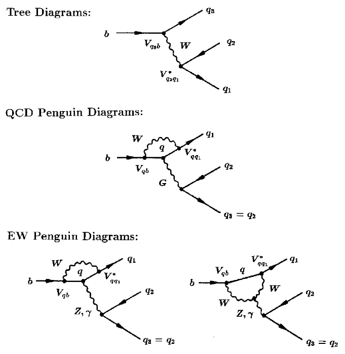
Figure 22: Lowest order contributions to non-leptonic $b$-quark decays $(q\in\{u,c,t\})$.

In view of such measurements starting at the end of this millennium it is mandatory to search for decays that should allow interesting insights both into the mechanism of CP violation and into the structure of electroweak interactions in general. Since non-leptonic $B$-meson decays play the central role in respect to CP violation and extracting angles of the unitarity triangle, let us have a closer look at these transitions in the following subsection.

8.2 Classification of Non-leptonic $B$ Decays and Low Energy Effective Hamiltonians

Non-leptonic $B$ decays are caused by $b$-quark transitions of the type $b\to q_{1}\,\overline{q}_{2}\,q_{3}$ with $q_{1}\in\{d,s\}$ and $q_{2},q_{3}\in\{u,d,c,s\}$ and can be divided into three classes:

• $q_{2}=q_{3}\in\{u,c\}$: both tree and penguin diagrams contribute.

• $q_{2}=q_{3}\in\{d,s\}$: only penguin diagrams contribute.

• $q_{2}\not=q_{3}\in\{u,c\}$: only tree diagrams contribute.

The corresponding lowest order Feynman diagrams are shown in fig. 22. As we have seen in section 2, there are two types of penguin topologies: gluonic (QCD) and electroweak (EW) penguins originating from strong and electroweak interactions, respectively. Such penguin diagrams play not only an important role in $K$-meson decays as we have seen in the previous sections but also in non-leptonic $B$ decays.

$$\begin{array}[]{|c|c|c|c|c|}\hline\cr\mbox{Quark-Decay}&\mbox{Exclusive Decay}&\mbox{Discussed in}&\mbox{Probe of}&\mbox{Cleanliness}\\ \hline\cr\hline\cr b\to d\bar{u}u&\begin{array}[]{c}B_{d}\to\pi^{+}\pi^{-}\\ B_{s}\to\rho^{0}K_{\mbox{{\scriptsize S}}}\end{array}&\begin{array}[]{l}\ref{Bdpipi-Alpha}\\ \ref{Bsrk-Gamma}\end{array}&\begin{array}[]{c}\alpha\\ \gamma\end{array}&\begin{array}[]{c}++\\ -\end{array}\\ \hline\cr b\to d\bar{c}c&\begin{array}[]{c}B_{d}\to D^{+}D^{-}\\ B_{s}\to J/\psi\,K_{\mbox{{\scriptsize S}}}\end{array}&\begin{array}[]{l}\ref{Bdpipi-Alpha}\\ \ref{gold}\end{array}&\begin{array}[]{c}\beta\\ \lambda^{2}\eta\end{array}&\begin{array}[]{c}++\\ +-\end{array}\\ \hline\cr b\to s\bar{u}u&\begin{array}[]{c}B_{u,d}\to\pi K\\ B_{s}\to K^{+}K^{-},K^{\ast+}K^{\ast-}\end{array}&\begin{array}[]{l}\ref{SIMalp-gam},\,\ref{SU3REL}\\ \ref{BsiLoDG},\,\ref{kkbar}\end{array}&\begin{array}[]{c}\alpha,\,\gamma\\ \gamma\end{array}&\begin{array}[]{c}+-\\ ++\end{array}\\ \hline\cr b\to s\bar{c}c&\begin{array}[]{c}B_{d}\to J/\psi\,K_{\mbox{{\scriptsize S}}}\\ B_{s}\to J/\psi\,\phi,D_{s}^{\ast+}D_{s}^{\ast-}\end{array}&\begin{array}[]{l}\ref{Beta-Ext}\\ \ref{gold}\end{array}&\begin{array}[]{c}\beta\\ \lambda^{2}\eta\end{array}&\begin{array}[]{c}+++\\ ++\end{array}\\ \hline\cr\end{array}$$

Table 24: Examples for non-leptonic $B$ decays belonging to decay class i) receiving both tree and penguin contributions.

$$\begin{array}[]{|c|c|c|c|c|}\hline\cr\mbox{Quark-Decay}&\mbox{Exclusive Decay}&\mbox{Discussed in}&\mbox{Probe of}&\mbox{Cleanliness}\\ \hline\cr\hline\cr b\to d\bar{s}s&\begin{array}[]{c}B_{d}\to K^{0}\overline{K^{0}}\end{array}&\begin{array}[]{l}\ref{Bdpipi-Alpha}\end{array}&\begin{array}[]{c}\mbox{QCD Pen's}\end{array}&\begin{array}[]{c}\mbox{}\end{array}\\ \hline\cr b\to s\bar{s}s&\begin{array}[]{c}B_{d}\to\phi\,K_{\mbox{{\scriptsize S}}}\end{array}&\begin{array}[]{l}\ref{Zoo}\end{array}&\begin{array}[]{c}\beta\end{array}&\begin{array}[]{c}++\end{array}\\ \hline\cr b\to s\bar{d}d&\begin{array}[]{c}B_{s}\to K^{0}\overline{K^{0}},\,K^{\ast 0}\overline{K^{\ast 0}}\end{array}&\begin{array}[]{l}\ref{BsiLoDG},\,\ref{kkbar}\end{array}&\begin{array}[]{c}\mbox{QCD Pen's}\end{array}&\begin{array}[]{c}\mbox{}\end{array}\\ \hline\cr\end{array}$$

Table 25: Examples for non-leptonic $B$ decays belonging to decay class ii) receiving only penguin contributions.

Concerning CP violation, decay classes i) and ii) are very promising. These modes, which are usually referred to as $|\Delta B|=1$, $\Delta C=\Delta U=0$ transitions, will hence play the major role in the present section. We have collected examples of exclusive decays belonging to these categories in tables 24 and 25. There we have listed where these modes are discussed in the present section and which weak phases they probe. We have also given a classification of their theoretical cleanliness in respect of extracting these quantities. To analyze such transitions we shall use appropriate low energy effective Hamiltonians calculated in renormalization group improved perturbation theory. In the case of $|\Delta B|=1$, $\Delta C=\Delta U=0$ transitions we have

$${\cal H}_{\mbox{{\scriptsize eff}}}={\cal H}_{\mbox{{\scriptsize eff}}}(\Delta B=-1)+{\cal H}_{\mbox{{\scriptsize eff}}}(\Delta B=-1)^{\dagger}$$ (8.3)

with

$${\cal H}_{\mbox{{\scriptsize eff}}}(\Delta B=-1)=\frac{G_{\mbox{{\scriptsize F}}}}{\sqrt{2}}\left[\sum\limits_{j=u,c}V_{jq}^{\ast}V_{jb}\left\{\sum\limits_{k=1}^{2}Q_{k}^{jq}\,C_{k}(\mu)+\sum\limits_{k=3}^{10}Q_{k}^{q}\,C_{k}(\mu)\right\}\right],$$ (8.4)

where $\mu={\cal O}(m_{b})$. In writing this effective Hamiltonian we have generalized the notation of subsection 2.5 in order to exhibit different cases. We have introduced two quark flavour labels $j$ and $q$ to parametrize $b\to j\bar{j}q$ quark level transitions, i.e. $q\in\{d,s\}$ distinguishes between $b\to d$ and $b\to s$ transitions, respectively. These labels will turn out to be useful for the following discussion. Consequently

• current-current operators:

  $$\begin{array}[]{rcl}Q_{1}^{jq}&=&(\bar{q}_{\alpha}j_{\beta})_{\mbox{{\scriptsize V--A}}}(\bar{j}_{\beta}b_{\alpha})_{\mbox{{\scriptsize V--A}}}\\ Q_{2}^{jq}&=&(\bar{q}_{\alpha}j_{\alpha})_{\mbox{{\scriptsize V--A}}}(\bar{j}_{\beta}b_{\beta})_{\mbox{{\scriptsize V--A}}}.\end{array}$$ (8.5)

• QCD penguin operators:

  $$\begin{array}[]{rcl}Q_{3}^{q}&=&(\bar{q}_{\alpha}b_{\alpha})_{\mbox{{\scriptsize V--A}}}\sum\limits_{q^{\prime}=u,d,s,c,b}(\bar{q}^{\prime}_{\beta}q^{\prime}_{\beta})_{\mbox{{\scriptsize V--A}}}\\ Q_{4}^{q}&=&(\bar{q}_{\alpha}b_{\beta})_{\mbox{{\scriptsize V--A}}}\sum\limits_{q^{\prime}=u,d,s,c,b}(\bar{q}^{\prime}_{\beta}q^{\prime}_{\alpha})_{\mbox{{\scriptsize V--A}}}\\ Q_{5}^{q}&=&(\bar{q}_{\alpha}b_{\alpha})_{\mbox{{\scriptsize V--A}}}\sum\limits_{q^{\prime}=u,d,s,c,b}(\bar{q}^{\prime}_{\beta}q^{\prime}_{\beta})_{\mbox{{\scriptsize V+A}}}\\ Q_{6}^{q}&=&(\bar{q}_{\alpha}b_{\beta})_{\mbox{{\scriptsize V--A}}}\sum\limits_{q^{\prime}=u,d,s,c,b}(\bar{q}^{\prime}_{\beta}q^{\prime}_{\alpha})_{\mbox{{\scriptsize V+A}}}.\end{array}$$ (8.6)

• EW penguin operators:

  $$\begin{array}[]{rcl}Q_{7}^{q}&=&\frac{3}{2}(\bar{q}_{\alpha}b_{\alpha})_{\mbox{{\scriptsize V--A}}}\sum\limits_{q^{\prime}=u,d,s,c,b}e_{q^{\prime}}(\bar{q}^{\prime}_{\beta}q^{\prime}_{\beta})_{\mbox{{\scriptsize V+A}}}\\ Q_{8}^{q}&=&\frac{3}{2}(\bar{q}_{\alpha}b_{\beta})_{\mbox{{\scriptsize V--A}}}\sum\limits_{q^{\prime}=u,d,s,c,b}e_{q^{\prime}}(\bar{q}_{\beta}^{\prime}q^{\prime}_{\alpha})_{\mbox{{\scriptsize V+A}}}\\ Q_{9}^{q}&=&\frac{3}{2}(\bar{q}_{\alpha}b_{\alpha})_{\mbox{{\scriptsize V--A}}}\sum\limits_{q^{\prime}=u,d,s,c,b}e_{q^{\prime}}(\bar{q}^{\prime}_{\beta}q^{\prime}_{\beta})_{\mbox{{\scriptsize V--A}}}\\ Q_{10}^{q}&=&\frac{3}{2}(\bar{q}_{\alpha}b_{\beta})_{\mbox{{\scriptsize V--A}}}\sum\limits_{q^{\prime}=u,d,s,c,b}e_{q^{\prime}}(\bar{q}^{\prime}_{\beta}q^{\prime}_{\alpha})_{\mbox{{\scriptsize V--A}}}.\end{array}$$ (8.7)

Let us stress that one has to be very careful using NLO Wilson coefficient functions. The point is that renormalization scheme dependences arising in $C_{k}(\mu)$ beyond LO require the inclusion of certain matrix elements calculated at $\mu={\cal O}(m_{b})$ in order to cancel this dependence [237, 238, 239]. Numerical values of the Wilson coefficient functions are given in table 26. We note the large value of the coefficient $C_{9}$. A remarkable feature of this coefficient is its very weak renormalization scheme dependence. We will see below that the operator $Q_{9}$ plays an important role in certain non-leptonic $B$ decays [238, 299, 300].

	$\Lambda_{\overline{\rm MS}}^{(5)}=160\,{\rm MeV}$			$\Lambda_{\overline{\rm MS}}^{(5)}=225\,{\rm MeV}$			$\Lambda_{\overline{\rm MS}}^{(5)}=290\,{\rm MeV}$
Scheme	LO	NDR	HV	LO	NDR	HV	LO	NDR	HV
$C_{1}$	-0.283	-0.171	-0.209	-0.308	-0.185	-0.228	-0.331	-0.198	-0.245
$C_{2}$	1.131	1.075	1.095	1.144	1.082	1.105	1.156	1.089	1.114
$C_{3}$	0.013	0.013	0.012	0.014	0.014	0.013	0.016	0.016	0.014
$C_{4}$	-0.028	-0.033	-0.027	-0.030	-0.035	-0.029	-0.032	-0.038	-0.032
$C_{5}$	0.008	0.008	0.008	0.009	0.009	0.009	0.009	0.009	0.010
$C_{6}$	-0.035	-0.037	-0.030	-0.038	-0.041	-0.033	-0.041	-0.045	-0.036
$C_{7}/\alpha$	0.043	-0.003	0.006	0.045	-0.002	0.005	0.047	-0.002	0.005
$C_{8}/\alpha$	0.043	0.049	0.055	0.048	0.054	0.060	0.053	0.059	0.065
$C_{9}/\alpha$	-1.268	-1.283	-1.273	-1.280	-1.292	-1.283	-1.290	-1.300	-1.293
$C_{10}/\alpha$	0.302	0.243	0.245	0.328	0.263	0.266	0.352	0.281	0.284

Table 26: $\Delta B=1$ Wilson coefficients at $\mu=\overline{m}_{\rm b}(m_{\rm b})=4.40\,{\rm GeV}$ for $m_{\rm t}=170\,{\rm GeV}$.

Decays belonging to class iii) allow in some cases clean extractions of the angle $\gamma$ of the unitarity triangle without any hadronic uncertainties and are therefore also very important. We have given examples of such modes in table 27. In the case of these transitions only current-current operators contribute. The structure of the corresponding low energy effective Hamiltonians is completely analogous to (8.4). We have simply to replace both the CKM factors $V_{jq}^{\ast}V_{jb}$ and the flavour contents of the current-current operators straightforwardly, and have to omit the sum over penguin operators. We shall come back to the resulting Hamiltonians in our discussion of $B_{s}$ decays originating from $\bar{b}\to\bar{u}c\bar{s}$ ($b\to c\bar{u}s$) quark-level transitions that is presented in 8.6.5.

Whereas CP-violating asymmetries in charged $B$ decays suffer in general from large hadronic uncertainties and are hence mainly interesting in respect of ruling out superweak models [100] of CP violation, the neutral $B_{q}$-meson systems $(q\in\{d,s\})$ provide excellent laboratories to perform stringent tests of the Standard Model description of CP violation [240]. This feature is mainly due to “mixing-induced” CP violation which is absent in the charged $B$ system and arises from interference between decay- and $B^{0}_{q}-\overline{B^{0}_{q}}$ mixing-processes. We have discussed $B^{0}_{q}-\overline{B^{0}_{q}}$ mixing briefly in subsection 4.3. In order to derive the formulae for the CP-violating asymmetries, we have to extend this discussion considerably.

$$\begin{array}[]{|c|c|c|c|c|}\hline\cr\mbox{Quark-Decay}&\mbox{Exclusive Decay}&\mbox{Discussed in}&\mbox{Probe of}&\mbox{Cleanliness}\\ \hline\cr\hline\cr b\to s\left\{\begin{array}[]{c}\bar{u}c\\ \bar{c}u\end{array}\right\}&\begin{array}[]{c}B_{s}\to D_{s}K,\,D\phi\\ B_{u,d}\to DK\end{array}&\begin{array}[]{l}\ref{nonCP}\\ \ref{BDKtri}\end{array}&\begin{array}[]{c}\gamma\\ \gamma\end{array}&\begin{array}[]{c}+++\\ +++\end{array}\\ \hline\cr\end{array}$$

Table 27: Examples for non-leptonic $B$ decays belonging to decay class iii) receiving only tree contributions. The corresponding exclusive $b\to d$ modes are not promising in respect of CP violation and the extraction of CKM phases since interference between the $b\to d\bar{u}c$ and $b\to d\bar{c}u$ amplitudes is highly CKM-suppressed.

8.3 More about $B^{0}_{q}-\overline{B^{0}_{q}}$ Mixing

Within the Standard Model, $B^{0}_{q}-\overline{B^{0}_{q}}$ mixing is induced at lowest order through the box diagrams shown in fig. 23. Applying a matrix notation, the Wigner-Weisskopf formalism [241] yields an effective Schrödinger equation of the form

$$i\,\frac{\partial}{\partial t}\left(\begin{array}[]{c}a(t)\\ b(t)\end{array}\right)=\left[\left(\begin{array}[]{cc}M_{0}^{(q)}&M_{12}^{(q)}\\ M_{12}^{(q)\ast}&M_{0}^{(q)}\end{array}\right)-\frac{i}{2}\left(\begin{array}[]{cc}\Gamma_{0}^{(q)}&\Gamma_{12}^{(q)}\\ \Gamma_{12}^{(q)\ast}&\Gamma_{0}^{(q)}\end{array}\right)\right]\cdot\left(\begin{array}[]{c}a(t)\\ b(t)\end{array}\right)$$ (8.8)

describing the time evolution of the state vector

$$\left|\psi_{q}(t)\right\rangle=a(t)\left|B^{0}_{q}\right\rangle+b(t)\left|\overline{B^{0}_{q}}\right\rangle.$$ (8.9)

The special form of the mass and decay matrices in (8.8) follows from invariance under CPT transformations. It is an easy exercise to evaluate the eigenstates $\left|B_{\pm}^{(q)}\right\rangle$ with eigenvalues $\lambda_{\pm}^{(q)}$ of that Hamilton operator. They are given by

$$\left|B_{\pm}^{(q)}\right\rangle=\frac{1}{\sqrt{1+|\alpha_{q}|^{2}}}\left(\left|B^{0}_{q}\right\rangle\pm\alpha_{q}\left|\overline{B^{0}_{q}}\right\rangle\right)$$ (8.10)

$$\lambda_{\pm}^{(q)}=\left(M_{0}^{(q)}-\frac{i}{2}\Gamma_{0}^{(q)}\right)\pm\left(M_{12}^{(q)}-\frac{i}{2}\Gamma_{12}^{(q)}\right)\alpha_{q},$$ (8.11)

where

$$\alpha_{q}=\sqrt{\frac{4|M_{12}^{(q)}|^{2}e^{-i2\delta\Theta_{M/\Gamma}^{(q)}}+|\Gamma_{12}^{(q)}|^{2}}{4|M_{12}^{(q)}|^{2}+|\Gamma_{12}^{(q)}|^{2}-4|M_{12}^{(q)}||\Gamma_{12}^{(q)}|\sin\delta\Theta_{M/\Gamma}^{(q)}}}e^{-i\left(\Theta_{\Gamma_{12}}^{(q)}+n^{\prime}\pi\right)}.$$ (8.12)

Here the notations $M_{12}^{(q)}\equiv e^{i\Theta_{M_{12}}^{(q)}}|M_{12}^{(q)}|$, $\Gamma_{12}^{(q)}\equiv e^{i\Theta_{\Gamma_{12}}^{(q)}}|\Gamma_{12}^{(q)}|$ and $\delta\Theta_{M/\Gamma}^{(q)}\equiv\Theta_{M_{12}}^{(q)}-\Theta_{\Gamma_{12}}^{(q)}$ have been introduced and $n^{\prime}\in{\rm Z}$ parametrizes the sign of the square root appearing in that expression. Calculating the dispersive and absorptive parts of the box diagrams depicted in fig. 23 one obtains [242]

$$M_{12}^{(q)}=\frac{G_{\mbox{{\scriptsize F}}}^{2}M_{W}^{2}\eta_{B}m_{B_{q}}B_{B_{q}}F_{B_{q}}^{2}}{12\pi^{2}}v_{t}^{(q)2}S_{0}(x_{t})\,e^{i(\pi-\phi_{\mbox{{\scriptsize CP}}}(B_{q}))}$$ (8.13)

and

$$\Gamma_{12}^{(q)}=\frac{G_{\mbox{{\scriptsize F}}}^{2}m_{b}^{2}m_{B_{q}}B_{B_{q}}F_{B_{q}}^{2}}{8\pi}\left[v_{t}^{(q)2}+\frac{8}{3}v_{c}^{(q)}v_{t}^{(q)}\left(z_{c}+\frac{1}{4}z_{c}^{2}-\frac{1}{2}z_{c}^{3}\right)\right.$$

$$+\left.v_{c}^{(q)2}\left\{\sqrt{1-4z_{c}}\left(1-\frac{2}{3}z_{c}\right)+\frac{8}{3}z_{c}+\frac{2}{3}z_{c}^{2}-\frac{4}{3}z_{c}^{3}-1\right\}\right]e^{-i\phi_{\mbox{{\scriptsize CP}}}(B_{q})},$$

respectively, where $x_{t}\equiv m_{t}^{2}/M_{W}^{2}$ and $z_{c}\equiv m_{c}^{2}/m_{b}^{2}$. As in subsection 4.3 we have retained only the top contribution to $M_{12}$. The charm contribution and the mixed top-charm contributions are entirely negligible. The non-perturbative parameter $B_{B_{q}}$ has been defined in (4.34). QCD corrections to (8.3), which have been omitted in that expression and are only known at LO [242, 247], play essentially no role for the following discussion of CP violation. In order to distinguish the CKM factors present in (8.13) and (8.3) from $\lambda_{i}=V_{is}^{\ast}V_{id}$ used in $K$ decays, we have introduced the notation

$$v_{i}^{(q)}\equiv V_{iq}^{\ast}V_{ib}$$ (8.15)

with $q=d,s$. Next the phase $\phi_{\mbox{{\scriptsize CP}}}(B_{q})$ parametrizing the applied CP phase convention is defined through

$$({\cal CP})\left|B^{0}_{q}\right\rangle=e^{i\phi_{\mbox{{\scriptsize CP}}}(B_{q})}\left|\overline{B^{0}_{q}}\right\rangle.$$ (8.16)

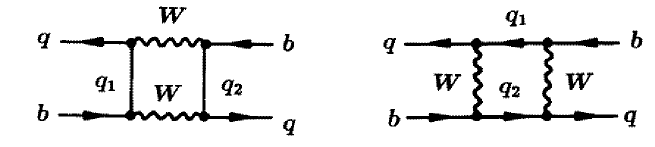
Figure 23: Box diagrams contributing to $B^{0}_{q}-\overline{B^{0}_{q}}$ mixing $(q_{1},q_{2}\in\{u,c,t\})$.

Since the expression (8.3) for the off-diagonal element $\Gamma_{12}^{(q)}$ of the decay matrix is similarly to $M_{12}^{(q)}$ dominated by the term proportional to $v_{t}^{(q)2}$, we have

$$\frac{\Gamma_{12}^{(q)}}{M_{12}^{(q)}}\approx-\frac{3\pi}{2S_{0}(x_{t})}\frac{m_{b}^{2}}{M_{W}^{2}}.$$ (8.17)

Therefore, $|\Gamma_{12}^{(q)}|/|M_{12}^{(q)}|={\cal O}(m_{b}^{2}/m_{t}^{2})\ll 1$. Expanding (8.12) in powers of this small quantity gives

$$\alpha_{q}=\left[1+\frac{|\Gamma_{12}^{(q)}|}{2|M_{12}^{(q)}|}\sin\delta\Theta_{M/\Gamma}^{(q)}\right]e^{-i\left(\Theta_{M_{12}}^{(q)}+n^{\prime}\pi\right)}+{\cal O}\left(\left(\frac{|\Gamma_{12}^{(q)}|}{|M_{12}^{(q)}|}\right)^{2}\right).$$ (8.18)

The deviation of $|\alpha_{q}|$ from 1 describes CP-violating effects in $B^{0}_{q}-\overline{B^{0}_{q}}$ oscillations. This type of CP violation is probed by rate asymmetries in semileptonic decays of neutral $B_{q}$-mesons into “wrong charge” leptons, i.e. by comparing the rate of an initially pure $B_{q}^{0}$-meson decaying into $l^{-}\overline{\nu}_{l}X$ with that of an initially pure $\overline{B^{0}_{q}}$ decaying into $l^{+}\nu_{l}X$:

$${\cal A}^{(q)}_{\mbox{{\scriptsize SL}}}\equiv\frac{\Gamma(B^{0}_{q}(t)\to l^{-}\overline{\nu}_{l}X)-\Gamma(\overline{B^{0}_{q}}(t)\to l^{+}\nu_{l}X)}{\Gamma(B^{0}_{q}(t)\to l^{-}\overline{\nu}_{l}X)+\Gamma(\overline{B^{0}_{q}}(t)\to l^{+}\nu_{l}X)}=\frac{|\alpha_{q}|^{4}-1}{|\alpha_{q}|^{4}+1}\approx\frac{|\Gamma_{12}^{(q)}|}{|M_{12}^{(q)}|}\sin\delta\Theta^{(q)}_{M/\Gamma}.$$ (8.19)

Note that the time dependences cancel in (8.19). Because of $|\Gamma_{12}^{(q)}|/|M_{12}^{(q)}|\propto m_{b}^{2}/m_{t}^{2}$ and $\sin\delta\Theta^{(q)}_{M/\Gamma}\propto m_{c}^{2}/m_{b}^{2}$, the asymmetry (8.19) is suppressed by a factor $m_{c}^{2}/m_{t}^{2}={\cal O}(10^{-4})$ and is hence expected to be very small within the Standard Model. At present there exists an experimental upper bound $|\mbox{Re}(\varepsilon_{B_{d}})|\equiv|{\cal A}^{(d)}_{\mbox{{\scriptsize SL}}}/4|<45\cdot 10^{-3}$ (90% C.L.) from the CLEO collaboration [243] which is about two orders of magnitudes above the Standard Model prediction.

The time-evolution of initially, i.e. at $t=0$, pure $\left|B^{0}_{q}\right\rangle$ and $\left|\overline{B^{0}_{q}}\right\rangle$ meson states is given by

$$\left|B^{0}_{q}(t)\right\rangle = f_{+}^{(q)}(t)\left|B^{0}_{q}\right\rangle+\alpha_{q}f_{-}^{(q)}(t)\left|\overline{B^{0}_{q}}\right\rangle$$ (8.20)

$$\left|\overline{B^{0}_{q}}(t)\right\rangle = \frac{1}{\alpha_{q}}f_{-}^{(q)}(t)\left|B^{0}_{q}\right\rangle+f_{+}^{(q)}(t)\left|\overline{B^{0}_{q}}\right\rangle,$$ (8.21)

where

$$f_{\pm}^{(q)}(t)=\frac{1}{2}\left(e^{-i\lambda_{+}^{(q)}t}\pm e^{-i\lambda_{-}^{(q)}t}\right).$$ (8.22)

Using these time-dependent state vectors and neglecting the very small CP-violating effects in $B^{0}_{q}-\overline{B^{0}_{q}}$ mixing that are described by $|\alpha_{q}|\not=1$ (see (8.18)), a straightforward calculation yields [244]

$$\Gamma(B^{0}_{q}(t)\to f) = \left[\left|g_{+}^{(q)}(t)\right|^{2}+\left|\xi_{f}^{(q)}\right|^{2}\left|g_{-}^{(q)}(t)\right|^{2}-2\mbox{\,Re}\left\{\xi_{f}^{(q)}g_{-}^{(q)}(t)g_{+}^{(q)}(t)^{\ast}\right\}\right]\tilde{\Gamma}$$ (8.23)

$$\Gamma(\overline{B^{0}_{q}}(t)\to f) = \left[\left|g_{-}^{(q)}(t)\right|^{2}+\left|\xi_{f}^{(q)}\right|^{2}\left|g_{+}^{(q)}(t)\right|^{2}-2\mbox{\,Re}\left\{\xi_{f}^{(q)}g_{+}^{(q)}(t)g_{-}^{(q)}(t)^{\ast}\right\}\right]\tilde{\Gamma}\quad$$ (8.24)

$$\Gamma(B^{0}_{q}(t)\to\overline{f}) = \left[\left|g_{+}^{(q)}(t)\right|^{2}+\left|\xi_{\overline{f}}^{(q)}\right|^{2}\left|g_{-}^{(q)}(t)\right|^{2}-2\mbox{\,Re}\left\{\xi_{\overline{f}}^{(q)}g_{-}^{(q)}(t)g_{+}^{(q)}(t)^{\ast}\right\}\right]\tilde{\overline{\Gamma}}$$ (8.25)

$$\Gamma(\overline{B^{0}_{q}}(t)\to\overline{f}) = \left[\left|g_{-}^{(q)}(t)\right|^{2}+\left|\xi_{\overline{f}}^{(q)}\right|^{2}\left|g_{+}^{(q)}(t)\right|^{2}-2\mbox{\,Re}\left\{\xi_{\overline{f}}^{(q)}g_{+}^{(q)}(t)g_{-}^{(q)}(t)^{\ast}\right\}\right]\tilde{\overline{\Gamma}},$$ (8.26)

where

$$\left|g^{(q)}_{\pm}(t)\right|^{2}=\frac{1}{4}\left[e^{-\Gamma_{L}^{(q)}t}+e^{-\Gamma_{H}^{(q)}t}\pm 2\,e^{-\Gamma_{q}t}\cos(\Delta M_{q}t)\right]$$ (8.27)

$$g_{-}^{(q)}(t)\,g_{+}^{(q)}(t)^{\ast}=\frac{1}{4}\left[e^{-\Gamma_{L}^{(q)}t}-e^{-\Gamma_{H}^{(q)}t}+2\,i\,e^{-\Gamma_{q}t}\sin(\Delta M_{q}t)\right]$$ (8.28)

and

$$\xi_{f}^{(q)}=e^{-i\Theta_{M_{12}}^{(q)}}\frac{A(\overline{B_{q}^{0}}\to f)}{A(B_{q}^{0}\to f)},\quad\xi_{\overline{f}}^{(q)}=e^{-i\Theta_{M_{12}}^{(q)}}\frac{A(\overline{B_{q}^{0}}\to\overline{f})}{A(B_{q}^{0}\to\overline{f})}.$$ (8.29)

In the time-dependent rates (8.23)-(8.26), the time-independent transition rates $\tilde{\Gamma}$ and $\tilde{\overline{\Gamma}}$ correspond to the “unevolved” decay amplitudes $A(B^{0}_{q}\to f)$ and $A(B^{0}_{q}\to\overline{f})$, respectively, and can be calculated by performing the usual phase space integrations. The functions $g_{\pm}^{(q)}(t)$ are related to $f_{\pm}^{(q)}(t)$. However, whereas the latter functions depend through $\alpha_{q}$ on the quantity $n^{\prime}$ parametrizing the sign of the square root appearing in (8.12), $g_{\pm}^{(q)}(t)$ and the rates (8.23)-(8.26) do not depend on that parameter. The $n^{\prime}$-dependence is cancelled by introducing the positive mass difference

$$\Delta M_{q}\equiv M_{H}^{(q)}-M_{L}^{(q)}=2\left|M_{12}^{(q)}\right|>0$$ (8.30)

of the $B_{q}$ mass eigenstates, where $H$ and $L$ refer to “heavy” and “light”, respectively. The quantities $\Gamma_{H}^{(q)}$ and $\Gamma_{L}^{(q)}$ denote the corresponding decay widths. Their difference can be expressed as

$$\Delta\Gamma_{q}\equiv\Gamma_{H}^{(q)}-\Gamma_{L}^{(q)}=\frac{4\mbox{\,Re}\left[M_{12}^{(q)}\Gamma_{12}^{(q)\ast}\right]}{\Delta M_{q}},$$ (8.31)

while the average decay width of the $B_{q}$ mass eigenstates is given by

$$\Gamma_{q}\equiv\frac{\Gamma^{(q)}_{H}+\Gamma^{(q)}_{L}}{2}=\Gamma^{(q)}_{0}.$$ (8.32)

Whereas both the mixing phase $\Theta_{M_{12}}^{(q)}$ and the amplitude ratios appearing in (8.29) depend on the chosen CP phase convention parametrized through $\phi_{\mbox{{\scriptsize CP}}}(B_{q})$, the quantities $\xi_{f}^{(q)}$ and $\xi_{\overline{f}}^{(q)}$ are convention independent observables. We shall see the cancellation of $\phi_{\mbox{{\scriptsize CP}}}(B_{q})$ explicitly in a moment.

The $B^{0}_{q}-\overline{B^{0}_{q}}$ mixing phase $\Theta_{M_{12}}^{(q)}$ appearing in the equations given above is essential for the later discussion of “mixing-induced” CP violation. As can be read off from the expression (8.13) for the off-diagonal element $M_{12}^{(q)}$ of the mass matrix, $\Theta_{M_{12}}^{(q)}$ is related to complex phases of CKM matrix elements through

$$\Theta_{M_{12}}^{(q)}=\pi+2\,\mbox{arg}\left(V_{tq}^{\ast}V_{tb}\right)-\phi_{\mbox{{\scriptsize CP}}}(B_{q}).$$ (8.33)

Note that the perturbative QCD corrections to $B^{0}_{q}-\overline{B^{0}_{q}}$ mixing represented by $\eta_{B}$ in (8.13) do not affect the mixing phase $\Theta_{M_{12}}^{(q)}$ and have therefore no significance for mixing-induced CP violation.

A measure of the strength of the $B^{0}_{q}-\overline{B^{0}_{q}}$ oscillations is provided by the “mixing parameter”

$$x_{q}\equiv\frac{\Delta M_{q}}{\Gamma_{q}}.$$ (8.34)

As discussed in section 4, the present ranges for $x_{d}$ and $x_{s}$ can be summarized as [71]

$$x_{q}=\left\{\begin{array}[]{ll}0.72\pm 0.03&\mbox{\quad for $q=d$}\\ \quad{\cal O}(20)&\mbox{\quad for $q=s$}\end{array}\right.$$ (8.35)

with $x_{s}={\cal O}(20)$ being the Standard Model expectation.

The mixing parameters listed in (8.35) have interesting phenomenological consequences for the width differences $\Delta\Gamma_{d,s}$ defined by (8.31). Using this expression we obtain

$$\frac{\Delta\Gamma_{q}}{\Gamma_{q}}\approx-\frac{3\pi}{2S(x_{t})}\frac{m_{b}^{2}}{M_{W}^{2}}\,x_{q}.$$ (8.36)

Consequently $\Delta\Gamma_{q}$ is negative so that the decay width $\Gamma_{H}^{(q)}$ of the “heavy” mixing eigenstate is smaller than that of the “light” eigenstate. Since the numerical factor in (8.36) multiplying the mixing parameter $x_{q}$ is ${\cal O}(10^{-2})$, the width difference $\Delta\Gamma_{d}$ is very small within the Standard Model. On the other hand, the expected large value of $x_{s}$ implies a sizable $\Delta\Gamma_{s}$ which may be as large as ${\cal O}(20\%)$. The dynamical origin of this width difference is related to CKM favored $\bar{b}\to\bar{c}c\bar{s}$ quark-level transitions into final states that are common to $B^{0}_{s}$ and $\overline{B^{0}_{s}}$ mesons. Theoretical analyses of $\Delta\Gamma_{s}/\Gamma_{s}$ indicate that it may indeed be as large as ${\cal O}(20\%)$. These studies are based on box diagram calculations [245], on a complementary approach where one sums over many exclusive $\bar{b}\to\bar{c}c\bar{s}$ modes [246], and on the Heavy Quark Expansion yielding the most recent result [247]

$$\frac{\Delta\Gamma_{s}}{\Gamma_{s}}=0.16^{+0.11}_{-0.09}\,.$$ (8.37)

This width difference can be determined experimentally e.g. from angular correlations in $B_{s}\to J/\psi\,\phi$ decays [248]. One expects $10^{3}-10^{4}$ reconstructed $B_{s}\to J/\psi\,\phi$ events both at Tevatron Run II and at HERA-B which may allow a precise measurement of $\Delta\Gamma_{s}$. As was pointed out by Dunietz [249], $\Delta\Gamma_{s}$ may lead to interesting CP-violating effects in untagged data samples of time-evolved $B_{s}$ decays where one does not distinguish between initially present $B^{0}_{s}$ and $\overline{B^{0}_{s}}$ mesons. Before we shall turn to detailed discussions of CP-violating asymmetries in the $B_{d}$ system and of the $B_{s}$ system in light of $\Delta\Gamma_{s}$, let us focus on $B_{q}$ decays ($q\in\{d,s\}$) into final CP eigenstates first. For an analysis of $B_{d}$ transitions into non CP eigenstates the reader is referred to [250], $B_{s}$ decays of this kind will be discussed in detail in 8.6.5.

8.4 $B_{q}$ Decays into CP Eigenstates

A very promising special case in respect of extracting CKM phases from CP-violating effects in neutral $B_{q}$ decays are transitions into final states $|f\rangle$ that are eigenstates of the CP operator and hence satisfy

$$({\cal CP})|f\rangle=\pm|f\rangle.$$ (8.38)

Consequently we have $\xi_{f}^{(q)}=\xi_{\overline{f}}^{(q)}$ in that case (see (8.29)) and have to deal only with a single observable $\xi_{f}^{(q)}$ containing essentially all the information that is needed to evaluate the time-dependent decay rates (8.23)-(8.26). Decays into final states that are not eigenstates of the CP operator play an important role in the case of the $B_{s}$ system to extract the UT angle $\gamma$ and are discussed in 8.6.5.

8.4.1 Calculation of $\xi_{f}^{(q)}$

Whereas the $B^{0}_{q}-\overline{B^{0}_{q}}$ mixing phase $\Theta_{M_{12}}^{(q)}$ entering the expression (8.29) for $\xi_{f}^{(q)}$ is simply given as a function of complex phases of certain CKM matrix elements (see (8.33)), the amplitude ratio $A(\overline{B^{0}_{q}}\to f)/A(B^{0}_{q}\to f)$ requires the calculation of hadronic matrix elements which are poorly known at present. In order to investigate this amplitude ratio, we shall employ the low energy effective Hamiltonian for $|\Delta B|=1$, $\Delta C=\Delta U=0$ transitions discussed in section 8.2. Using (8.4) we get

$$A\left(\overline{B^{0}_{q}}\to f\right)=\Bigl{\langle}f\Bigl{|}{\cal H}_{\mbox{{\scriptsize eff}}}(\Delta B=-1)\Bigr{|}\overline{B^{0}_{q}}\Bigr{\rangle}$$

$$=\Biggl{\langle}f\left|\frac{G_{\mbox{{\scriptsize F}}}}{\sqrt{2}}\left[\sum\limits_{j=u,c}V_{jr}^{\ast}V_{jb}\left\{\sum\limits_{k=1}^{2}Q_{k}^{jr}(\mu)C_{k}(\mu)+\sum\limits_{k=3}^{10}Q_{k}^{r}(\mu)C_{k}(\mu)\right\}\right]\right|\overline{B^{0}_{q}}\Biggr{\rangle},$$

where the flavour label $r\in\{d,s\}$ distinguishes – as in the whole subsection – between $b\to d$ and $b\to s$ transitions. On the other hand, the transition amplitude $A\left(B^{0}_{q}\to f\right)$ is given by

$$A\left(B^{0}_{q}\to f\right)=\left\langle f\left|{\cal H}_{\mbox{{\scriptsize eff}}}(\Delta B=-1)^{\dagger}\right|B^{0}_{q}\right\rangle$$

$$=\Biggl{\langle}f\left|\frac{G_{\mbox{{\scriptsize F}}}}{\sqrt{2}}\left[\sum\limits_{j=u,c}V_{jr}V_{jb}^{\ast}\left\{\sum\limits_{k=1}^{2}Q_{k}^{jr\dagger}(\mu)C_{k}(\mu)+\sum\limits_{k=3}^{10}Q_{k}^{r\dagger}(\mu)C_{k}(\mu)\right\}\right]\right|B^{0}_{q}\Biggr{\rangle}.$$

Performing appropriate CP transformations in this equation, i.e. inserting the operator $({\cal CP})^{\dagger}({\cal CP})=\hat{1}$ both after the bra $\langle f|$ and in front of the ket $|B^{0}_{q}\rangle$, yields

$$A\left(B^{0}_{q}\to f\right)=\pm e^{i\phi_{\mbox{{\scriptsize CP}}}(B_{q})}$$

$$\times\Biggl{\langle}f\left|\frac{G_{\mbox{{\scriptsize F}}}}{\sqrt{2}}\left[\sum\limits_{j=u,c}V_{jr}V_{jb}^{\ast}\left\{\sum\limits_{k=1}^{2}Q_{k}^{jr}(\mu)C_{k}(\mu)+\sum\limits_{k=3}^{10}Q_{k}^{r}(\mu)C_{k}(\mu)\right\}\right]\right|\overline{B^{0}_{q}}\Biggr{\rangle},$$

where we have applied the relation

$$({\cal CP})Q_{k}^{jr\dagger}({\cal CP})^{\dagger}=Q_{k}^{jr}$$ (8.42)

and have furthermore taken into account (8.16) and (8.38). Consequently we obtain

$$\frac{A(\overline{B^{0}_{q}}\to f)}{A(B^{0}_{q}\to f)}=\pm\,e^{-i\phi_{\mbox{{\scriptsize CP}}}(B_{q})}\,\frac{\sum\limits_{j=u,c}v_{j}^{(r)}\Bigl{\langle}f\Bigl{|}{\cal Q}^{jr}\Bigr{|}\overline{B^{0}_{q}}\Bigr{\rangle}}{\sum\limits_{j=u,c}v_{j}^{(r)\ast}\Bigl{\langle}f\Bigl{|}{\cal Q}^{jr}\Bigr{|}\overline{B^{0}_{q}}\Bigr{\rangle}},$$ (8.43)

where $v_{j}^{(r)}\equiv V_{jr}^{\ast}V_{jb}$ and the operators ${\cal Q}^{jr}$ are defined by

$${\cal Q}^{jr}\equiv\sum\limits_{k=1}^{2}Q_{k}^{jr}C_{k}(\mu)+\sum\limits_{k=3}^{10}Q_{k}^{r}C_{k}(\mu).$$ (8.44)

Inserting (8.33) and (8.43) into the expression (8.29) for $\xi_{f}^{(q)}$, we observe explicitly that the convention dependent phases $\phi_{\mbox{{\scriptsize CP}}}(B_{q})$ appearing in the former two equations cancel each other and arrive at the convention independent result

$$\xi_{f}^{(q)}=\mp\,e^{-i\phi_{\mbox{{\scriptsize M}}}^{(q)}}\frac{\sum\limits_{j=u,c}v_{j}^{(r)}\Bigl{\langle}f\Bigl{|}{\cal Q}^{jr}\Bigr{|}\overline{B^{0}_{q}}\Bigr{\rangle}}{\sum\limits_{j=u,c}v_{j}^{(r)\ast}\Bigl{\langle}f\Bigl{|}{\cal Q}^{jr}\Bigr{|}\overline{B^{0}_{q}}\Bigr{\rangle}}.$$ (8.45)

Here the phase $\phi_{\mbox{{\scriptsize M}}}^{(q)}\equiv 2\,\mbox{arg}(V_{tq}^{\ast}V_{tb})$ arises from the $B^{0}_{q}-\overline{B^{0}_{q}}$ mixing phase $\Theta_{M_{12}}^{(q)}$. Applying the modified Wolfenstein parametrization (8.1), $\phi_{\mbox{{\scriptsize M}}}^{(q)}$ can be related to angles of the unitarity triangle as follows:

$$\phi_{\mbox{{\scriptsize M}}}^{(q)}=\left\{\begin{array}[]{cl}2\beta&\mbox{for $q=d$}\\ 0&\mbox{for $q=s$.}\end{array}\right.$$ (8.46)

Consequently a non-trivial mixing phase arises only in the $B_{d}$ system.

In general the observable $\xi_{f}^{(q)}$ suffers from large hadronic uncertainties that are introduced through the hadronic matrix elements appearing in (8.45). However, there is a very important special case where these uncertainties cancel and theoretical clean predictions of $\xi_{f}^{(q)}$ are possible.

8.4.2 Dominance of a Single CKM Amplitude

If the transition matrix elements appearing in (8.45) are dominated by a single CKM amplitude, the observable $\xi_{f}^{(q)}$ takes the very simple form

$$\xi_{f}^{(q)}=\mp\exp\left[-i\left\{\phi_{\mbox{{\scriptsize M}}}^{(q)}-\phi_{\mbox{{\scriptsize D}}}^{(f)}\right\}\right],$$ (8.47)

where the characteristic “decay” phase $\phi_{\mbox{{\scriptsize D}}}^{(f)}$ can be expressed in terms of angles of the unitarity triangle as follows:

$$\phi_{\mbox{{\scriptsize D}}}^{(f)}=\left\{\begin{array}[]{cl}-2\gamma&\mbox{for dominant $\bar{b}\to\bar{u}u\bar{r}$ CKM amplitudes in $B_{q}^{0}\to f$}\\ 0&\mbox{for dominant $\bar{b}\to\bar{c}c\bar{r}$\,\, CKM amplitudes in $B_{q}^{0}\to f$.}\end{array}\right.$$ (8.48)

The validity of dominance of a single CKM amplitude and important phenomenological applications of (8.47) will be discussed in the following subsections.

8.5 The $B_{d}$ System

In contrast to the $B_{s}$ system, the width difference is negligibly small in the $B_{d}$ system. Consequently the expressions for the decay rates (8.23)-(8.26) simplify considerably in that case.

8.5.1 CP Asymmetries in $B_{d}$ Decays

Restricting ourselves, as in the previous subsection, to decays into final CP eigenstates $|f\rangle$ satisfying (8.38), we obtain the following expressions for the time-dependent and time-integrated CP asymmetries:

$$a_{\mbox{{\scriptsize CP}}}(B_{d}\to f;t)\equiv\frac{\Gamma(B_{d}^{0}(t)\to f)-\Gamma(\overline{B_{d}^{0}}(t)\to f)}{\Gamma(B_{d}^{0}(t)\to f)+\Gamma(\overline{B_{d}^{0}}(t)\to f)}$$ (8.49)

$$={\cal A}_{\mbox{{\scriptsize CP}}}^{\mbox{{\scriptsize dir}}}(B_{d}\to f)\cos(\Delta M_{d}t)+{\cal A}_{\mbox{{\scriptsize CP}}}^{\mbox{{\scriptsize mix-ind}}}(B_{d}\to f)\sin(\Delta M_{d}t)$$

$$a_{\mbox{{\scriptsize CP}}}(B_{d}\to f)\equiv\frac{\int\limits_{0}^{\infty}\mbox{d}t\left[\Gamma(B_{d}^{0}(t)\to f)-\Gamma(\overline{B_{d}^{0}}(t)\to f)\right]}{\int\limits_{0}^{\infty}\mbox{d}t\left[\Gamma(B_{d}^{0}(t)\to f)+\Gamma(\overline{B_{d}^{0}}(t)\to f)\right]}$$ (8.50)

$$=\frac{1}{1+x_{d}^{2}}\left[{\cal A}_{\mbox{{\scriptsize CP}}}^{\mbox{{\scriptsize dir}}}(B_{d}\to f)+x_{d}\,{\cal A}_{\mbox{{\scriptsize CP}}}^{\mbox{{\scriptsize mix-ind}}}(B_{d}\to f)\right],$$

where the direct CP-violating contributions

$${\cal A}_{\mbox{{\scriptsize CP}}}^{\mbox{{\scriptsize dir}}}(B_{d}\to f)\equiv\frac{1-\left|\xi_{f}^{(d)}\right|^{2}}{1+\left|\xi_{f}^{(d)}\right|^{2}}$$ (8.51)

have been separated from the mixing-induced CP-violating contributions

$${\cal A}_{\mbox{{\scriptsize CP}}}^{\mbox{{\scriptsize mix-ind}}}(B_{d}\to f)\equiv\frac{2\,\mbox{Im}\,\xi_{f}^{(d)}}{1+\left|\xi_{f}^{(d)}\right|^{2}}.$$ (8.52)

Whereas the former observables describe CP violation arising directly in the corresponding decay amplitudes, the latter ones are due to interference between $B^{0}_{d}-\overline{B^{0}_{d}}$ mixing- and decay-processes. Needless to say, the expressions (8.49) and (8.50) have to be modified appropriately for the $B_{s}$ system because of $\Delta\Gamma_{s}/\Gamma_{s}={\cal O}(20\%)$. In the case of the time-dependent CP asymmetry (8.49) these effects start to become important for $t\,\mbox{{\scriptsize$\stackrel{{\scriptstyle>}}{{\sim}}$}}\,2/\Delta\Gamma_{s}$.

8.5.2 CP Violation in $B_{d}\to J/\psi\,K_{\mbox{{\scriptsize S}}}$: the “Gold-plated” Way to Extract $\beta$

The channel $B_{d}\to J/\psi\,K_{\mbox{{\scriptsize S}}}$ is a transition into a CP eigenstate with eigenvalue $-1$ and originates from a $\bar{b}\to\bar{c}c\bar{s}$ quark-level decay [251]. Consequently the corresponding observable $\xi^{(d)}_{\psi K_{\mbox{{\scriptsize S}}}}$ can be expressed as

$$\xi^{(d)}_{\psi K_{\mbox{{\scriptsize S}}}}=+e^{-2i\beta}\left[\frac{v_{u}^{(s)}A^{ut^{\prime}}_{\mbox{{\scriptsize pen}}}+v_{c}^{(s)}\left(A_{\mbox{{\scriptsize cc}}}^{c^{\prime}}+A^{ct^{\prime}}_{\mbox{{\scriptsize pen}}}\right)}{v_{u}^{(s)\ast}A^{ut^{\prime}}_{\mbox{{\scriptsize pen}}}+v_{c}^{(s)\ast}\left(A_{\mbox{{\scriptsize cc}}}^{c^{\prime}}+A^{ct^{\prime}}_{\mbox{{\scriptsize pen}}}\right)}\right],$$ (8.53)

where $A_{\mbox{{\scriptsize cc}}}^{c^{\prime}}$ denotes the $Q_{1,2}^{cs}$ current-current operator amplitude and $A^{ut^{\prime}}_{\mbox{{\scriptsize pen}}}$ $(A^{ct^{\prime}}_{\mbox{{\scriptsize pen}}})$ corresponds to contributions of the penguin-type with up- and top-quarks (charm- and top-quarks) running as virtual particles in the loops. Note that within this notation penguin-like matrix elements of the $Q_{1,2}^{cs}$ current-current operators are included by definition in the $A^{ct^{\prime}}_{\mbox{{\scriptsize pen}}}$ amplitude, whereas those of $Q_{1,2}^{us}$ show up in $A^{ut^{\prime}}_{\mbox{{\scriptsize pen}}}$. The primes in (8.53) have been introduced to remind us that we are dealing with a $\bar{b}\to\bar{s}$ mode. Using the modified Wolfenstein parametrization (8.1), the relevant CKM factors take the form

$$v_{u}^{(s)}=A\lambda^{4}R_{b}\,e^{-i\gamma},\quad v_{c}^{(s)}=A\lambda^{2}\left(1-\lambda^{2}/2\right)$$ (8.54)

and imply that the $A^{ut^{\prime}}_{\mbox{{\scriptsize pen}}}$ contribution is highly CKM suppressed with respect to the part containing the current-current amplitude. The suppression factor is given by

$$\left|v_{u}^{(s)}/v_{c}^{(s)}\right|=\lambda^{2}R_{b}\approx 0.02.$$ (8.55)

An additional suppression arises from the fact that $A^{ut^{\prime}}_{\mbox{{\scriptsize pen}}}$ is related to loop processes that are governed by Wilson coefficients of ${\cal O}(10^{-2})$. Moreover the colour-structure of $B_{d}\to J/\psi\,K_{\mbox{{\scriptsize S}}}$ leads to further suppression! The point is that the $\bar{c}$- and $c$-quarks emerging from the gluons of the usual QCD penguin diagrams form a colour-octet state and consequently cannot build up the $J/\psi$ which is a $\bar{c}c$ colour-singlet state. Therefore additional gluons are needed. Their contributions are unfortunately very hard to estimate. However, the former colour-argument does not hold for EW penguins which may hence be the most important penguin contributions to $B_{d}\to J/\psi\,K_{\mbox{{\scriptsize S}}}$. The suppression of $v_{u}^{(s)}A_{\mbox{{\scriptsize pen}}}^{ut^{\prime}}$ relative to $v_{c}^{(s)}(A_{\mbox{{\scriptsize cc}}}^{c^{\prime}}+A_{\mbox{{\scriptsize pen}}}^{ct^{\prime}})$ is compensated slightly since the dominant $Q_{1,2}^{cs}$ current-current amplitude $A_{\mbox{{\scriptsize cc}}}^{c^{\prime}}$ is colour-suppressed by a phenomenological colour-suppression factor $a_{2}\approx 0.2$ [252]-[254]. However, since $v_{u}^{(s)}A_{\mbox{{\scriptsize pen}}}^{ut^{\prime}}$ is suppressed by three sources (CKM-structure, loop effects, colour-structure), we conclude that $\xi^{(d)}_{\psi K_{\mbox{{\scriptsize S}}}}$ is nevertheless given to an excellent approximation by

$$\xi^{(d)}_{\psi K_{\mbox{{\scriptsize S}}}}=e^{-2i\beta}\left[\frac{v_{c}^{(s)}\left(A_{\mbox{{\scriptsize cc}}}^{c^{\prime}}+A^{ct^{\prime}}_{\mbox{{\scriptsize pen}}}\right)}{v_{c}^{(s)\ast}\left(A_{\mbox{{\scriptsize cc}}}^{c^{\prime}}+A^{ct^{\prime}}_{\mbox{{\scriptsize pen}}}\right)}\right]=e^{-2i\beta}$$ (8.56)

yielding

$${\cal A}_{\mbox{{\scriptsize CP}}}^{\mbox{{\scriptsize dir}}}(B_{d}\to J/\psi\,K_{\mbox{{\scriptsize S}}})=0,\quad{\cal A}_{\mbox{{\scriptsize CP}}}^{\mbox{{\scriptsize mix-ind}}}(B_{d}\to J/\psi\,K_{\mbox{{\scriptsize S}}})=-\sin(2\beta)$$ (8.57)

and thus

$$a_{\mbox{{\scriptsize CP}}}(B_{d}\to J/\psi\,K_{\mbox{{\scriptsize S}}};t)=-\sin(2\beta)\,\sin(\Delta M_{d}t)$$ (8.58)

$$a_{\mbox{{\scriptsize CP}}}(B_{d}\to J/\psi\,K_{\mbox{{\scriptsize S}}})=-\frac{x_{d}}{1+x_{d}^{2}}\,\sin(2\beta)$$ (8.59)

for the time-dependent and time-integrated CP asymmetries (8.49) and (8.50), respectively. Consequently these observables measure $\sin(2\beta)$ to excellent accuracy. Therefore $B_{d}\to J/\psi\,K_{\mbox{{\scriptsize S}}}$ is usually referred to as the “gold-plated” mode to determine the UT angle $\beta$. The presently expected ranges for $\sin(2\beta)$ can be read off from table 5 and imply non zero values for the CP-violating asymmetries (8.58) and (8.59). The latter asymmetry is expected to be of the order $-30\%$ within the Standard Model. Other methods for extracting $\beta$ can be found e.g. in [250, 255].

8.5.3 CP Violation in $B_{d}\to\pi^{+}\pi^{-}$ and Extractions of $\alpha$

In the case of $B_{d}\to\pi^{+}\pi^{-}$ we have to deal with the decay of a $B_{d}$-meson into a final CP eigenstate with eigenvalue $+1$ that is caused by the quark-level process $\bar{b}\to\bar{u}u\bar{d}$. Therefore we may write

$$\xi^{(d)}_{\pi^{+}\pi^{-}}=-e^{-2i\beta}\left[\frac{v_{u}^{(d)}\left(A_{\mbox{{\scriptsize cc}}}^{u}+A^{ut}_{\mbox{{\scriptsize pen}}}\right)+v_{c}^{(d)}A^{ct}_{\mbox{{\scriptsize pen}}}}{v_{u}^{(d)\ast}\left(A_{\mbox{{\scriptsize cc}}}^{u}+A^{ut}_{\mbox{{\scriptsize pen}}}\right)+v_{c}^{(d)\ast}A^{ct}_{\mbox{{\scriptsize pen}}}}\right],$$ (8.60)

where the notation of decay amplitudes is as in the previous discussion of $B_{d}\to J/\psi\,K_{\mbox{{\scriptsize S}}}$. Using again (8.1), the CKM factors are given by

$$v_{u}^{(d)}=A\lambda^{3}R_{b}\,e^{-i\gamma},\quad v_{c}^{(d)}=-A\lambda^{3}.$$ (8.61)

The CKM structure of (8.60) is very different form $\xi^{(d)}_{\psi K_{\mbox{{\scriptsize S}}}}$. In particular the pieces containing the dominant $Q_{1,2}^{ud}$ current-current contributions $A_{\mbox{{\scriptsize cc}}}^{u}$ are CKM suppressed with respect to the penguin contributions $A^{ct}_{\mbox{{\scriptsize pen}}}$ by

$$\left|v_{u}^{(d)}/v_{c}^{(d)}\right|=R_{b}\approx 0.36\,.$$ (8.62)

In contrast to $B_{d}\to J/\psi\,K_{\mbox{{\scriptsize S}}}$, in the $B_{d}\to\pi^{+}\pi^{-}$ case the penguin amplitudes are only suppressed by the corresponding Wilson coefficients ${\cal O}(10^{-2})$ and not additionally by the colour-structure of that decay. Taking into account that the current-current amplitude $A_{\mbox{{\scriptsize cc}}}^{u}$ is colour-allowed and using both (8.62) and characteristic values of the Wilson coefficient functions, one obtains

$$\left|\frac{v_{c}^{(d)}A^{ct}_{\mbox{{\scriptsize pen}}}}{v_{u}^{(d)}\left(A_{\mbox{{\scriptsize cc}}}^{u}+A^{ut}_{\mbox{{\scriptsize pen}}}\right)}\right|={\cal O}(0.15)$$ (8.63)

and concludes that

$$\xi^{(d)}_{\pi^{+}\pi^{-}}\approx-e^{-2i\beta}\left[\frac{v_{u}^{(d)}\left(A_{\mbox{{\scriptsize cc}}}^{u}+A^{ut}_{\mbox{{\scriptsize pen}}}\right)}{v_{u}^{(d)\ast}\left(A_{\mbox{{\scriptsize cc}}}^{u}+A^{ut}_{\mbox{{\scriptsize pen}}}\right)}\right]=-e^{2i\alpha}$$ (8.64)

may be a reasonable approximation to obtain an estimate for the UT angle $\alpha$ from the CP-violating observables

$${\cal A}_{\mbox{{\scriptsize CP}}}^{\mbox{{\scriptsize dir}}}(B_{d}\to\pi^{+}\pi^{-})\approx 0,\quad{\cal A}_{\mbox{{\scriptsize CP}}}^{\mbox{{\scriptsize mix-ind}}}(B_{d}\to\pi^{+}\pi^{-})\approx-\sin(2\alpha)$$ (8.65)

implying the following time-dependent and time-integrated CP asymmetries (8.49) and (8.50):

$$a_{\mbox{{\scriptsize CP}}}(B_{d}\to\pi^{+}\pi^{-};t)\approx-\sin(2\alpha)\,\sin(\Delta M_{d}t)$$ (8.66)

$$a_{\mbox{{\scriptsize CP}}}(B_{d}\to\pi^{+}\pi^{-})\approx-\frac{x_{d}}{1+x_{d}^{2}}\,\sin(2\alpha)\,.$$ (8.67)

Note that a measurement of ${\cal A}_{\mbox{{\scriptsize CP}}}^{\mbox{{\scriptsize dir}}}(B_{d}\to\pi^{+}\pi^{-})\not=0$, i.e. of a contribution to (8.66) evolving with $\cos(\Delta M_{d}t)$, would signal the presence of penguins. We shall come back to this feature later.

The formalism discussed above can also be applied straightforwardly to $B_{d}\to D^{+}D^{-}$ (caused by $\bar{b}\to\bar{c}c\bar{d}$) that is dominated by the contributions proportional to $v_{c}^{(d)}$. In that case (8.62) leads to an additional suppression of the $v_{u}^{(d)}$ amplitude originating essentially from penguin contributions. Consequently the relations

$${\cal A}_{\mbox{{\scriptsize CP}}}^{\mbox{{\scriptsize dir}}}(B_{d}\to D^{+}D^{-})=0,\quad{\cal A}_{\mbox{{\scriptsize CP}}}^{\mbox{{\scriptsize mix-ind}}}(B_{d}\to D^{+}D^{-})=\sin(2\beta)$$ (8.68)

are expected to be satisfied to higher accuracy than (8.65). However, in respect of theoretical cleanliness to extract $\beta$, the decay $B_{d}\to D^{+}D^{-}$ cannot compete with the “gold-plated” mode $B_{d}\to J/\psi\,K_{\mbox{{\scriptsize S}}}$.

The hadronic uncertainties affecting the extraction of $\alpha$ from CP violation in $B_{d}\to\pi^{+}\pi^{-}$ were analyzed by many authors in the literature. A selection of papers is given in [256, 257]. As was pointed out by Gronau and London [258], the uncertainties related to QCD penguins [259] can be eliminated with the help of isospin relations involving in addition to $B_{d}\to\pi^{+}\pi^{-}$ also the modes $B_{d}\to\pi^{0}\pi^{0}$ and $B^{\pm}\to\pi^{\pm}\pi^{0}$. The isospin relations among the corresponding decay amplitudes are given by

$$A(B^{0}_{d}\to\pi^{+}\pi^{-})+\sqrt{2}A(B^{0}_{d}\to\pi^{0}\pi^{0}) = \sqrt{2}A(B^{+}\to\pi^{+}\pi^{0})$$ (8.69)

$$A(\overline{B^{0}_{d}}\to\pi^{+}\pi^{-})+\sqrt{2}A(\overline{B^{0}_{d}}\to\pi^{0}\pi^{0}) = \sqrt{2}A(B^{-}\to\pi^{-}\pi^{0})$$ (8.70)

and can be represented as two triangles in the complex plane that allow the extraction of a value of $\alpha$ that does not suffer from QCD penguin uncertainties. It is, however, not possible to control also the EW penguin uncertainties using that isospin approach. The point is that up- and down-quarks are coupled differently in EW penguin diagrams because of their different electrical charges (see (8.7)). Hence one has also to think about the role of these contributions. We shall come back to that issue in subsection 9.3, where a more detailed discussion of the GL method [258] in light of EW penguin effects will be given.

An experimental problem of the GL method is related to the fact that it requires a measurement of $Br(B_{d}\to\pi^{0}\pi^{0})$ which may be smaller than ${\cal O}(10^{-6})$ because of colour-suppression effects [260]. Therefore, despite of its attractiveness, that approach may be quite difficult from an experimental point of view and it is important to have alternatives available to determine $\alpha$. Needless to say, that is also required in order to over-constrain the UT angle $\alpha$ as much as possible at future $B$-physics experiments. Fortunately such methods are already on the market. For example, Snyder and Quinn suggested to use $B\to\rho\,\pi$ modes to extract $\alpha$ [261]. Another method was proposed in [262]. It requires a simultaneous measurement of ${\cal A}_{\mbox{{\scriptsize CP}}}^{\mbox{{\scriptsize mix-ind}}}(B_{d}\to\pi^{+}\pi^{-})$ and ${\cal A}_{\mbox{{\scriptsize CP}}}^{\mbox{{\scriptsize mix-ind}}}(B_{d}\to K^{0}\overline{K^{0}})$ and determines $\alpha$ with the help of a geometrical triangle construction using the $SU(3)$ flavour symmetry of strong interactions. The accuracy of that approach is limited by $SU(3)$-breaking corrections which cannot be estimated reliably at present. Interestingly the penguin-induced decay $B_{d}\to K^{0}\overline{K^{0}}$ may exhibit CP asymmetries as large as ${\cal O}(30\%)$ within the Standard Model [263]. This feature is due to interference between QCD penguins with internal up- and charm-quark exchanges [264]. In the absence of these contributions, the CP-violating asymmetries of $B_{d}\to K^{0}\overline{K^{0}}$ would vanish and “New Physics” would be required (see e.g. [265]) to induce CP violation in that decay. An upper bound $Br(B_{d}\to K^{0}\overline{K^{0}})<1.7\cdot 10^{-5}$ has been presented very recently by the CLEO collaboration [266].

Before discussing other methods to deal with the penguin uncertainties affecting the extraction of $\alpha$ from the CP-violating observables of $B_{d}\to\pi^{+}\pi^{-}$, let us next have a closer look at the above mentioned QCD penguins with up- and charm-quarks running as virtual particles in the loops.

8.5.4 Penguin Zoology

The general structure of a generic $\bar{b}\to\bar{q}$ ($q\in\{d,s\}$) penguin amplitude is given by

$$P^{(q)}=V_{uq}V_{ub}^{\ast}\,P_{u}^{(q)}+V_{cq}V_{cb}^{\ast}\,P_{c}^{(q)}+V_{tq}V_{tb}^{\ast}\,P_{t}^{(q)},$$ (8.71)

where $P_{u}^{(q)}$, $P_{c}^{(q)}$ and $P_{t}^{(q)}$ are the amplitudes of penguin processes with internal up-, charm- and top-quark exchanges, respectively, omitting CKM factors. The penguin amplitudes introduced in (8.53) and (8.60) are related to these quantities through

$$\begin{array}[]{rclcrcl}A^{ut}_{\mbox{{\scriptsize pen}}}&=&P_{u}^{(d)}-P_{t}^{(d)},&&A^{ct}_{\mbox{{\scriptsize pen}}}&=&P_{c}^{(d)}-P_{t}^{(d)}\\ A^{ut^{\prime}}_{\mbox{{\scriptsize pen}}}&=&P_{u}^{(s)}-P_{t}^{(s)},&&A^{ct^{\prime}}_{\mbox{{\scriptsize pen}}}&=&P_{c}^{(s)}-P_{t}^{(s)}.\end{array}$$ (8.72)

Using unitarity of the CKM matrix yields

$$P^{(q)}=V_{cq}V_{cb}^{\ast}\left[P_{c}^{(q)}-P_{u}^{(q)}\right]+V_{tq}V_{tb}^{\ast}\left[P_{t}^{(q)}-P_{u}^{(q)}\right],$$ (8.73)

where the CKM factors can be expressed with the help of the Wolfenstein parametrization as follows:

$$V_{cd}V_{cb}^{\ast}=-\lambda|V_{cb}|\left(1+{\cal O}\left(\lambda^{4}\right)\right),\quad V_{td}V_{tb}^{\ast}=|V_{td}|e^{-i\beta},$$ (8.74)

$$V_{cs}V_{cb}^{\ast}=|V_{cb}|\left(1+{\cal O}\left(\lambda^{2}\right)\right),\quad V_{ts}V_{tb}^{\ast}=-|V_{cb}|\left(1+{\cal O}\left(\lambda^{2}\right)\right).\quad$$ (8.75)

The estimate of the non-leading terms in $\lambda$ follows Subsection 3.3. Omitting these terms and combining (8.73) with (8.74) and (8.75), the $\bar{b}\to\bar{d}$ and $\bar{b}\to\bar{s}$ penguin amplitudes take the form

$$P^{(d)}=\left[e^{-i\beta}-\frac{1}{R_{t}}\Delta P^{(d)}\right]\left|V_{td}\right|\left|P_{tu}^{(d)}\right|e^{i\delta_{tu}^{(d)}}$$ (8.76)

$$P^{(s)}=\left[1-\Delta P^{(s)}\right]e^{-i\pi}\left|V_{cb}\right|\left|P_{tu}^{(s)}\right|e^{i\delta_{tu}^{(s)}},$$ (8.77)

where the notation

$$P_{q_{1}q_{2}}^{(q)}\equiv P_{q_{1}}^{(q)}-P_{q_{2}}^{(q)}$$ (8.78)

has been introduced and

$$\Delta P^{(q)}\equiv\frac{P^{(q)}_{cu}}{P^{(q)}_{tu}}$$ (8.79)

describes the contributions of “subdominant” penguins with up- and charm-quarks running as virtual particles in the loops. In the limit of degenerate up- and charm-quark masses, $\Delta P^{(q)}$ would vanish because of the GIM mechanism [17]. However, since $m_{u}\approx 4.5$ MeV, whereas $m_{c}\approx 1.4$ GeV, this GIM cancellation is incomplete and in principle sizable effects arising from $\Delta P^{(q)}$ could be expected.

Figure 24: The dependence of $\left|\Delta P^{(q)}\right|$ on $k^{2}/m_{b}^{2}$.

Usually it is assumed that the penguin amplitudes (8.76) and (8.77) are dominated by internal top-quark exchanges, i.e. $\Delta P^{(q)}\approx 0$. That is an excellent approximation for EW penguin contributions which play an important role in certain $B$ decays only because of the large top-quark mass as we will see in section 9. However, QCD penguins with internal up- and charm-quarks may become important as is indicated by model calculations at the perturbative quark-level [264]. Following the pioneering approach of Bander, Silverman and Soni [267], the strong phase of $\Delta P^{(q)}$ is generated exclusively through absorptive parts of time-like penguin diagrams with internal up- and charm-quark exchanges. These estimates of $\Delta P^{(q)}$ depend strongly on the value of $k^{2}$ denoting the four-momentum of the gluon appearing in the time-like QCD penguin diagrams. This feature can be seen nicely in fig. 24, where that dependence is shown. Simple kinematical considerations at the quark-level imply that $k^{2}$ should lie within the “physical” range [237, 268, 269]

$$\frac{1}{4}\,\mbox{{\scriptsize$\stackrel{{\scriptstyle<}}{{\sim}}$}}\,\frac{k^{2}}{m_{b}^{2}}\,\mbox{{\scriptsize$\stackrel{{\scriptstyle<}}{{\sim}}$}}\,\frac{1}{2}.$$ (8.80)

A detailed discussion of the $k^{2}$-dependence can be found in [269].

Looking at fig. 24, we observe that $\Delta P^{(q)}$ may lead to sizable effects for such values of $k^{2}$. Moreover QCD penguin topologies with internal up- and charm-quarks contain also long-distance contributions, like the rescattering process $B^{0}_{d}\to\{D^{+}D^{-}\}\to\pi^{+}\pi^{-}$ (see e.g. [270]), which are very hard to estimate. This feature can be seen easily by drawing the corresponding Feynman diagrams. Such long-distance contributions were discussed in the context of extracting $V_{td}$ from radiative $B$ decays in [271] and are potentially very serious. Consequently it may not be justified to neglect the $\Delta P^{(q)}$ terms in (8.76) and (8.77) [264]. Recently, in a different context, the importance of the $\Delta P^{(q)}$ contributions has been stressed in [272].

An important difference arises, however, between (8.76) and (8.77). While the UT angle $\beta$ shows up in the $\bar{b}\to\bar{d}$ case, there is only a trivial CP-violating weak phase present in the $\bar{b}\to\bar{s}$ case. Consequently $\Delta P^{(s)}$ cannot change the general phase structure of the $\bar{b}\to\bar{s}$ penguin amplitude $P^{(s)}$. On the other hand, if one takes into account also QCD penguins with internal up- and charm-quarks, the $\bar{b}\to\bar{d}$ penguin amplitude $P^{(d)}$ is no longer related in a simple and “clean” way through

$$P^{(d)}=e^{-i\beta}e^{i\delta_{P}^{(d)}}\left|P^{(d)}\right|$$ (8.81)

to $\beta$, where $\delta_{P}^{(d)}$ is a CP-conserving strong phase. As we pointed out in [264], this feature may affect some of the strategies to extract CKM phases with the help of $SU(3)$ amplitude relations that will be discussed later in this review.

An interesting consequence of (8.77) is the relation $P^{(s)}=\overline{P^{(s)}}$ between the $\bar{b}\to\bar{s}$ QCD penguin amplitude and its charge-conjugate implying that penguin-induced modes of this type, e.g. the decay $B_{d}\to\phi\,K_{\mbox{{\scriptsize S}}}$, should exhibit no direct CP violation. Applying the formalism developed in Subsection 8.4, one finds that

$${\cal A}_{\mbox{{\scriptsize CP}}}^{\mbox{{\scriptsize mix-ind}}}(B_{d}\to\phi\,K_{\mbox{{\scriptsize S}}})=-\sin(2\beta)$$ (8.82)

measures the angle $\beta$. Within the Standard Model, small direct CP violation – model calculations (see e.g. [238, 239, 269]) indicate asymmetries at the ${\cal O}(1\%)$ level – may arise from the neglected ${\cal O}(\lambda^{2})$ terms in (8.75) which also limit the theoretical accuracy of (8.82). An experimental comparison between the mixing-induced CP asymmetries of $B_{d}\to J/\psi\,K_{\mbox{{\scriptsize S}}}$ and $B_{d}\to\phi\,K_{\mbox{{\scriptsize S}}}$, which should be equal to very good accuracy within the Standard Model, would be extremely interesting since the latter decay is a “rare” FCNC process and may hence be very sensitive to physics beyond the Standard Model [8]. Recently this point has been discussed in more detail by London and Soni [273]. The branching ratio for $B_{d}\to\phi\,K_{\mbox{{\scriptsize S}}}$ is expected to be of ${\cal O}(10^{-5})$ and may be large enough to perform these measurements at future $B$ physics facilities.

8.5.5 Another Look at $B_{d}\to\pi^{+}\pi^{-}$ and the Extraction of $\alpha$

The discussion presented above implies that it is important to reanalyze the decay $B_{d}\to\pi^{+}\pi^{-}$ without assuming dominance of QCD penguins with internal top-quark exchanges. Such a study was performed in [274] (see also [272]). To this end it is useful to introduce

$$T\equiv V_{ud}V_{ub}^{\ast}\,A_{\mbox{{\scriptsize cc}}}^{u}$$ (8.83)

and to expand the CP-violating observables (8.51) and (8.52) corresponding to $B_{d}\to\pi^{+}\pi^{-}$ in powers of $\overline{P^{(d)}}/T$ and $P^{(d)}/T$, which we expect to satisfy the estimate [274]

$$\left|\frac{\overline{P^{(d)}}}{T}\right|\approx\left|\frac{P^{(d)}}{T}\right|\approx 0.07-0.23,$$ (8.84)

and to keep only the leading terms in that expansion:

$${\cal A}_{\mbox{{\scriptsize CP}}}^{\mbox{{\scriptsize dir}}}(B_{d}\to\pi^{+}\pi^{-})=2\lambda R_{t}\frac{|\tilde{P}|}{|T|}\sin\delta\sin\alpha+{\cal O}\left((P^{(d)}/T)^{2}\right)$$ (8.85)

$${\cal A}_{\mbox{{\scriptsize CP}}}^{\mbox{{\scriptsize mix-ind}}}(B_{d}\to\pi^{+}\pi^{-})$$

$$\qquad=-\sin 2\alpha-2\lambda R_{t}\frac{|\tilde{P}|}{|T|}\cos\delta\,\cos 2\alpha\,\sin\alpha+{\cal O}\left((P^{(d)}/T)^{2}\right).$$ (8.86)

Similar expressions were also derived by Gronau in [256]. However, it has not been assumed in (8.85) and (8.86) that QCD penguins are dominated by internal top-quark exchanges and the physical interpretation of the amplitude $\tilde{P}$ is quite different from [256]. This quantity is given by

$$\tilde{P}\equiv\left[1-\Delta P^{(d)}\right]|V_{cb}|\left|P_{tu}^{(d)}\right|e^{i\delta_{tu}^{(d)}}\,,$$ (8.87)

and $\delta$ appearing in (8.85) and (8.86) is simply the CP-conserving strong phase of $\tilde{P}/T$. If we compare (8.87) with (8.76) and (8.77), we observe that it is not equal to the amplitude $P^{(d)}$ – as one would expect naively – but that its phase structure corresponds exactly to the $\bar{b}\to\bar{s}$ QCD penguin amplitude $e^{i\pi}P^{(s)}$.

The two CP-violating observables (8.85) and (8.86) depend on the three “unknowns” $\alpha$, $\delta$ and $|\tilde{P}|/|T|$ (strategies to extract the CKM factor $R_{t}$ are discussed in previous sections and $\lambda$ is the usual Wolfenstein parameter). Consequently an additional input is needed to determine $\alpha$ from (8.85) and (8.86). Taking into account the discussion given in the previous paragraph, it is very natural to use the $SU(3)$ flavour symmetry of strong interactions to accomplish this task. In the strict $SU(3)$ limit one does not distinguish between down- and strange-quarks and $|\tilde{P}|$ corresponds simply to the magnitude of the decay amplitude of a penguin-induced $\bar{b}\to\bar{s}$ transition such as $B^{+}\to\pi^{+}K^{0}$ with an expected branching ratio of ${\cal O}(10^{-5})$ [260]. That decay has been measured very recently by the CLEO collaboration [266] with the branching ratio $Br(B^{+}\to\pi^{+}K^{0})=\left(2.3^{+1.1+0.2}_{-1.0-0.2}\pm 0.2\right)\cdot 10^{-5}$. On the other hand, $|T|$ can be estimated from the rate of $B^{+}\to\pi^{+}\pi^{0}$ by neglecting colour-suppressed current-current operator contributions. Presently only the upper bound $Br(B^{+}\to\pi^{+}\pi^{0})<2.0\cdot 10^{-5}$ is available for that mode [266].

Following these lines one obtains

$$\frac{|\tilde{P}|}{|T|}\approx\frac{F_{\pi}}{F_{K}}\sqrt{\frac{1}{2}\frac{Br(B^{+}\to\pi^{+}K^{0})}{Br(B^{+}\to\pi^{+}\pi^{0})}},$$ (8.88)

where $F_{\pi}$ and $F_{K}$ are the $\pi$- and $K$-meson decay constants, respectively, taking into account factorizable $SU(3)$-breaking. That relation allows the extraction both of $\alpha$ and $\delta$ from the measured CP-violating observables (8.85) and (8.86). Problems of this approach arise if $\alpha$ is close to $45^{\circ}$ or $135^{\circ}$, where the expansion (8.86) for ${\cal A}_{\mbox{{\scriptsize CP}}}^{\mbox{{\scriptsize mix-ind}}}(B_{d}\to\pi^{+}\pi^{-})$ breaks down. Assuming a total theoretical uncertainty of 30% in the quantity

$$a\equiv 2\lambda R_{t}\frac{|\tilde{P}|}{|T|}\approx 2\lambda R_{t}\frac{F_{\pi}}{F_{K}}\sqrt{\frac{1}{2}\frac{Br(B^{+}\to\pi^{+}K^{0})}{Br(B^{+}\to\pi^{+}\pi^{0})}}$$ (8.89)

governing (8.85) and (8.86), an uncertainty of $\pm\,3^{\circ}$ in the extracted value of $\alpha$ is expected if $\alpha$ is not too close to these singular points [274]. For values of $\alpha$ far away from $45^{\circ}$ and $135^{\circ}$, one may even have an uncertainty of only $\pm\,1^{\circ}$ as is indicated by the following example: Let us assume that the CP asymmetries are measured to be ${\cal A}_{\mbox{{\scriptsize CP}}}^{\mbox{{\scriptsize dir}}}(B_{d}\to\pi^{+}\pi^{-})=+\,0.1$ and ${\cal A}_{\mbox{{\scriptsize CP}}}^{\mbox{{\scriptsize mix-ind}}}(B_{d}\to\pi^{+}\pi^{-})=-\,0.25$ and that (8.89) gives $a=0.26$. Assuming a theoretical uncertainty of 30% in $a$, i.e. $\Delta a=\pm 0.04$, and inserting these numbers into (8.85) and (8.86) gives $\alpha=(76\pm 1)^{\circ}$ and $\delta=(24\pm 4)^{\circ}$. On the other hand, a naive analysis using (8.65) where the penguin contributions are neglected would yield $\alpha=83^{\circ}$. Consequently the theoretical uncertainty of the extracted value of $\alpha$ is expected to be significantly smaller than the shift through the penguin contributions. Since this method of extracting $\alpha$ requires neither difficult measurements of very small branching ratios nor complicated geometrical constructions it may turn out to be very useful for the early days of the $B$-factory era beginning at the end of this millennium.

8.5.6 A Simultaneous Extraction of $\alpha$ and $\gamma$

Recently it has been pointed out by Dighe, Gronau and Rosner that a time-dependent measurement of $B_{d}\to\pi^{+}\pi^{-}$ in combination with the branching ratios for $B^{0}_{d}\to\pi^{-}K^{+}$, $B^{+}\to\pi^{+}K^{0}$ and their charge-conjugates may allow a simultaneous determination of the angles $\alpha$ and $\gamma$ [275]. These decays provide the following six observables $A_{1},\ldots,A_{6}$:

$$\Gamma(B^{0}_{d}(t)\to\pi^{+}\pi^{-})+\Gamma(\overline{B^{0}_{d}}(t)\to\pi^{+}\pi^{-}) = e^{-\Gamma_{d}t}\,A_{1}$$ (8.90)

$$\Gamma(B^{0}_{d}(t)\to\pi^{+}\pi^{-})-\Gamma(\overline{B^{0}_{d}}(t)\to\pi^{+}\pi^{-}) = e^{-\Gamma_{d}t}\left[A_{2}\cos(\Delta M_{d}t)\right.$$ (8.91)

$$\quad+\left.A_{3}\sin(\Delta M_{d}t)\right]$$

$$\Gamma(B^{0}_{d}\to\pi^{-}K^{+})+\Gamma(\overline{B^{0}_{d}}\to\pi^{+}K^{-}) = A_{4}$$ (8.92)

$$\Gamma(B^{0}_{d}\to\pi^{-}K^{+})-\Gamma(\overline{B^{0}_{d}}\to\pi^{+}K^{-}) = A_{5}$$ (8.93)

$$\Gamma(B^{+}\to\pi^{+}K^{0})+\Gamma(B^{-}\to\pi^{-}\overline{K^{0}}) = A_{6}.$$ (8.94)

Using $SU(3)$ flavour symmetry of strong interactions, neglecting annihilation amplitudes, which should be suppressed by ${\cal O}(F_{B_{d}}/m_{B_{d}})$ with $F_{B_{d}}\approx 180\,\mbox{MeV}$, and assuming moreover that the $\bar{b}\to\bar{d}$ QCD penguin amplitude is related in a simple way to $\beta$ through (8.81), i.e. assuming top-quark dominance, the observables $A_{1},\ldots,A_{6}$ can be expressed in terms of six “unknowns” including $\alpha$ and $\gamma$. However, as we have outlined above, it is questionable whether the last assumption is justified since (8.81) may be affected by QCD penguins with internal up- and charm-quark exchanges [264]. Consequently the method proposed in [275] suffers from theoretical limitations. Nevertheless it is an interesting approach, probably mainly in view of constraining $\gamma$ which is the angle of the unitarity triangle that is most difficult to measure. In order to extract that angle, $B_{s}$ decays play an important role as we will see in the following subsection.

8.6 The $B_{s}$ System

The major phenomenological differences between the $B_{d}$ and $B_{s}$ systems arise from their mixing parameters (8.35) and from the fact that at leading order in the Wolfenstein expansion only a trivial weak mixing phase (8.46) is present in the $B_{s}$ case.

8.6.1 CP Violation in $B_{s}\to\rho^{0}K_{\mbox{{\scriptsize S}}}$: the “Wrong” Way to Extract $\gamma$

Let us begin our discussion of the $B_{s}$ system by having a closer look at the transition $B_{s}\to\rho^{0}K_{\mbox{{\scriptsize S}}}$ which appears frequently in the literature as a tool to extract $\gamma$. It is a $B_{s}$ decay into a final CP eigenstate with eigenvalue $-1$ that is (similarly as the $B_{d}\to\pi^{+}\pi^{-}$ mode) caused by the quark-level process $\bar{b}\to\bar{u}u\bar{d}$. Hence the corresponding observable $\xi^{(s)}_{\rho^{0}K_{\mbox{{\scriptsize S}}}}$ can be expressed as

$$\xi^{(s)}_{\rho^{0}K_{\mbox{{\scriptsize S}}}}=+e^{-i0}\left[\frac{v_{u}^{(d)}\left({\cal A}_{\mbox{{\scriptsize cc}}}^{u}+{\cal A}^{ut}_{\mbox{{\scriptsize pen}}}\right)+v_{c}^{(d)}{\cal A}^{ct}_{\mbox{{\scriptsize pen}}}}{v_{u}^{(d)\ast}\left({\cal A}_{\mbox{{\scriptsize cc}}}^{u}+{\cal A}^{ut}_{\mbox{{\scriptsize pen}}}\right)+v_{c}^{(d)\ast}{\cal A}^{ct}_{\mbox{{\scriptsize pen}}}}\right],$$ (8.95)

where the notation is as in 8.5.3. The structure of (8.95) is very similar to that of the observable $\xi^{(d)}_{\pi^{+}\pi^{-}}$ given in (8.60). However, an important difference arises between $B_{d}\to\pi^{+}\pi^{-}$ and $B_{s}\to\rho^{0}K_{\mbox{{\scriptsize S}}}$: although the penguin contributions are expected to be of equal order of magnitude in (8.60) and (8.95), their importance is enhanced in the latter case since the current-current amplitude ${\cal A}_{\mbox{{\scriptsize cc}}}^{u}$ is colour-suppressed by a phenomenological colour-suppression factor $a_{2}\approx 0.2$ [252]-[254]. Consequently, using in addition to that value of $a_{2}$ characteristic Wilson coefficient functions for the penguin operators and (8.62) for the ratio of CKM factors, one obtains

$$\left|\frac{v_{c}^{(d)}{\cal A}^{ct}_{\mbox{{\scriptsize pen}}}}{v_{u}^{(d)}\left({\cal A}_{\mbox{{\scriptsize cc}}}^{u}+{\cal A}^{ut}_{\mbox{{\scriptsize pen}}}\right)}\right|={\cal O}(0.5).$$ (8.96)

This estimate implies that

$$\xi^{(s)}_{\rho^{0}K_{\mbox{{\scriptsize S}}}}\approx+e^{-i0}\left[\frac{v_{u}^{(d)}\left({\cal A}_{\mbox{{\scriptsize cc}}}^{u}+{\cal A}^{ut}_{\mbox{{\scriptsize pen}}}\right)}{v_{u}^{(d)\ast}\left({\cal A}_{\mbox{{\scriptsize cc}}}^{u}+{\cal A}^{ut}_{\mbox{{\scriptsize pen}}}\right)}\right]=e^{-2i\gamma}$$ (8.97)

is a very bad approximation which should not allow a meaningful determination of $\gamma$ from the mixing-induced CP-violating asymmetry arising in $B_{s}\to\rho^{0}K_{\mbox{{\scriptsize S}}}$. Needless to note, the branching ratio of that decay is expected to be of ${\cal O}(10^{-7})$ which makes its experimental investigation very difficult. Interestingly there are other $B_{s}$ decays – some of them receive also penguin contributions – which do allow extractions of $\gamma$. Some of these strategies are even theoretically clean and suffer from no hadronic uncertainties. Before focussing on these modes, let us discuss an experimental problem of $B_{s}$ decays that is related to time-dependent measurements.

8.6.2 The $B_{s}$ System in Light of $\Delta\Gamma_{s}$

The large mixing parameter $x_{s}={\cal O}(20)$ that is expected within the Standard Model implies very rapid $B^{0}_{s}-\overline{B^{0}_{s}}$ oscillations requiring an excellent vertex resolution system to keep track of the $\Delta M_{s}t$ terms. That is obviously a formidable experimental task. It may, however, not be necessary to trace the rapid $\Delta M_{s}t$ oscillations in order to shed light on the mechanism of CP violation [249]. This remarkable feature is due to the expected sizable width difference $\Delta\Gamma_{s}$ which has been discussed at the end of subsection 8.3. Because of that width difference already untagged $B_{s}$ rates, which are defined by

$$\Gamma[f(t)]\equiv\Gamma(B_{s}^{0}(t)\to f)+\Gamma(\overline{B^{0}_{s}}(t)\to f),$$ (8.98)

may provide valuable information about the phase structure of the observable $\xi_{f}^{(s)}$. This can be seen nicely by rewriting (8.98) with the help of (8.23) and (8.24) in a more explicit way as follows:

$$\Gamma[f(t)]\propto\left[\left(1+\left|\xi_{f}^{(s)}\right|^{2}\right)\left(e^{-\Gamma_{L}^{(s)}t}+e^{-\Gamma_{H}^{(s)}t}\right)-2\mbox{\,Re\,}\xi_{f}^{(s)}\left(e^{-\Gamma_{L}^{(s)}t}-e^{-\Gamma_{H}^{(s)}t}\right)\right].$$ (8.99)

In this expression the rapid oscillatory $\Delta M_{s}t$ terms, which show up in the tagged rates (8.23) and (8.24), cancel [249]. Therefore it depends only on the two exponents $e^{-\Gamma_{L}^{(s)}t}$ and $e^{-\Gamma_{H}^{(s)}t}$. From an experimental point of view, such untagged analyses are clearly much more promising than tagged ones in respect of efficiency, acceptance and purity.

In order to illustrate these untagged rates in more detail, let us consider an estimate of $\gamma$ using untagged $B_{s}\to K^{+}K^{-}$ and $B_{s}\to K^{0}\overline{K^{0}}$ decays that has been proposed recently in [276]. Using the $SU(2)$ isospin symmetry of strong interactions to relate the QCD penguin contributions to these decays (EW penguins are colour-suppressed in these modes and should therefore play a minor role as we will see in section 9), we obtain

$$\Gamma[K^{+}K^{-}(t)]\propto|P^{\prime}|^{2}\Bigl{[}\bigl{(}1-2\,|r|\cos\varrho\,\cos\gamma+|r|^{2}\cos^{2}\gamma\bigr{)}e^{-\Gamma_{L}^{(s)}t}+|r|^{2}\sin^{2}\gamma\,e^{-\Gamma_{H}^{(s)}t}\Bigr{]}$$ (8.100)

and

$$\Gamma[K^{0}\overline{K^{0}}(t)]\propto|P^{\prime}|^{2}\,e^{-\Gamma_{L}^{(s)}t},$$ (8.101)

where

$$r\equiv|r|e^{i\varrho}=\frac{|T^{\prime}|}{|P^{\prime}|}e^{i(\delta_{T^{\prime}}-\delta_{P^{\prime}})}.$$ (8.102)

Here we have used the same notation as Gronau et al. in [277] which will turn out to be very useful for later discussions: $P^{\prime}$ denotes the $\bar{b}\to\bar{s}$ QCD penguin amplitude corresponding to (8.77), $T^{\prime}$ is the colour-allowed $\bar{b}\to\bar{u}u\bar{s}$ current-current amplitude, and $\delta_{P^{\prime}}$ and $\delta_{T^{\prime}}$ denote the corresponding CP-conserving strong phases. The primes remind us that we are dealing with $\bar{b}\to\bar{s}$ amplitudes. In order to determine $\gamma$ from the untagged rates (8.100) and (8.101), we need an additional input that is provided by the $SU(3)$ flavour symmetry of strong interactions. Using that symmetry and neglecting as in (8.88) the colour-suppressed current-current contributions to $B^{+}\to\pi^{+}\pi^{0}$, one finds [277]

$$|T^{\prime}|\approx\lambda\,\frac{F_{K}}{F_{\pi}}\,\sqrt{2}\,|A(B^{+}\to\pi^{+}\pi^{0})|,$$ (8.103)

where $\lambda$ is the usual Wolfenstein parameter, $F_{K}/F_{\pi}$ takes into account factorizable $SU(3)$-breaking, and $A(B^{+}\to\pi^{+}\pi^{0})$ denotes the appropriately normalized decay amplitude of $B^{+}\to\pi^{+}\pi^{0}$. Since $|P^{\prime}|$ is known from the untagged $B_{s}\to K^{0}\,\overline{K^{0}}$ rate (8.101), the quantity $|r|=|T^{\prime}|/|P^{\prime}|$ can be estimated with the help of (8.103) and allows the extraction of $\gamma$ from the part of (8.100) evolving with exponent $e^{-\Gamma_{H}^{(s)}t}$. As we will see in a moment, one can even do better, i.e. without using an $SU(3)$-based estimate like (8.103), by considering the decays corresponding to $B_{s}\to K\overline{K}$ where two vector mesons or appropriate higher resonances are present in the final states [276].

8.6.3 $\gamma$ from $B_{s}\to K^{\ast+}K^{\ast-}$ and $B_{s}\to K^{\ast 0}\overline{K^{\ast 0}}$

The untagged angular distributions of these decays, which take the general form

$$[f(\theta,\phi,\psi;t)]=\sum_{k}\left[\overline{b^{(k)}}(t)+b^{(k)}(t)\right]g^{(k)}(\theta,\phi,\psi),$$ (8.104)

provide many more observables than the untagged modes $B_{s}\to K^{+}K^{-}$ and $B_{s}\to K^{0}\overline{K^{0}}$ discussed in 8.6.2. Here $\theta$, $\phi$ and $\psi$ are generic decay angles describing the kinematics of the decay products arising in the decay chain $B_{s}\to K^{\ast}(\to\pi K)\,\overline{K^{\ast}}(\to\pi\overline{K})$. The observables $\left[\overline{b^{(k)}}(t)+b^{(k)}(t)\right]$ governing the time-evolution of the untagged angular distribution (8.104) are given by real or imaginary parts of bilinear combinations of decay amplitudes that are of the following structure:

$$\left[A_{\tilde{f}}^{\ast}(t)\,A_{f}(t)\right]\equiv\left\langle\left(K^{\ast}\overline{K^{\ast}}\right)_{\tilde{f}}\left|{\cal H}_{\mbox{{\scriptsize eff}}}\right|\overline{B_{s}^{0}}(t)\right\rangle^{\ast}\left\langle\left(K^{\ast}\overline{K^{\ast}}\right)_{f}\left|{\cal H}_{\mbox{{\scriptsize eff}}}\right|\overline{B_{s}^{0}}(t)\right\rangle$$ (8.105)

$$+\left\langle\left(K^{\ast}\overline{K^{\ast}}\right)_{\tilde{f}}\left|{\cal H}_{\mbox{{\scriptsize eff}}}\right|B_{s}^{0}(t)\right\rangle^{\ast}\left\langle\left(K^{\ast}\overline{K^{\ast}}\right)_{f}\left|{\cal H}_{\mbox{{\scriptsize eff}}}\right|B_{s}^{0}(t)\right\rangle.$$

In this expression, $f$ and $\tilde{f}$ are labels that define the relative polarizations of $K^{\ast}$ and $\overline{K^{\ast}}$ in final state configurations $\left(K^{\ast}\overline{K^{\ast}}\right)_{f}$ (e.g. linear polarization states [278] $\{0,\parallel,\perp\}$) with CP eigenvalues $\eta_{\mbox{{\scriptsize CP}}}^{f}$:

$$({\cal CP})\left|\left(K^{\ast}\overline{K^{\ast}}\right)_{f}\right\rangle=\eta_{\mbox{{\scriptsize CP}}}^{f}\left|\left(K^{\ast}\overline{K^{\ast}}\right)_{f}\right\rangle.$$ (8.106)

An analogous relation holds for $\tilde{f}$. The observables of the angular distributions for $B_{s}\to K^{\ast+}K^{\ast-}$ and $B_{s}\to K^{\ast 0}\overline{K^{\ast 0}}$ are given explicitly in [276]. In the case of the latter decay the formulae simplify considerably since it is a penguin-induced $\bar{b}\to\bar{s}d\bar{d}$ mode and receives therefore no tree contributions. Using, as in (8.100) and (8.101), the $SU(2)$ isospin symmetry of strong interactions, the QCD penguin contributions to $B_{s}\to K^{\ast+}K^{\ast-}$ and $B_{s}\to K^{\ast 0}\overline{K^{\ast 0}}$ can be related to each other. If one takes into account these relations and goes very carefully through the observables of the corresponding untagged angular distributions, one finds that they allow the extraction of $\gamma$ without any additional theoretical input [276]. In particular no $SU(3)$ symmetry arguments are needed and the $SU(2)$ isospin symmetry suffices to accomplish this task. The angular distributions provide moreover information about the hadronization dynamics of the corresponding decays, and the formalism developed for $B_{s}\to K^{\ast+}K^{\ast-}$ applies also to $B_{s}\to\rho^{0}\phi$ if one performs a suitable replacement of variables [276]. Since that channel is expected to be dominated by EW penguins as discussed in 9.2.3, it may allow interesting insights into the physics of these operators.

8.6.4 $B_{s}\to D_{s}^{\ast+}D_{s}^{\ast-}$ and $B_{s}\to J/\psi\,\phi$: “Gold-plated” Transitions to Extract $\eta$

The following discussion is devoted to an analysis [276] of the decays $B_{s}\to D_{s}^{\ast+}(\to D_{s}^{+}\gamma)\,D_{s}^{\ast-}(\to D_{s}^{-}\gamma)$ and $B_{s}\to J/\psi(\to l^{+}l^{-})\,\phi(\to K^{+}K^{-})$, which is the counterpart of the “gold-plated” mode $B_{d}\to J/\psi\,K_{\mbox{{\scriptsize S}}}$ to measure $\beta$. Since these decays are dominated by a single CKM amplitude, the hadronic uncertainties cancel in $\xi_{f}^{(s)}$ (see 8.4.2) taking in that particular case the following form:

$$\xi_{f}^{(s)}=-\eta_{\mbox{{\scriptsize CP}}}^{f}\,e^{i\,\phi_{\mbox{{\scriptsize CKM}}}}\,.$$ (8.107)

Consequently the observables of the untagged angular distributions, which have the same general structure as (8.104), simplify considerably [276]. In (8.107), $f$ is – as in (8.105) and (8.106) – a label defining the relative polarizations of $X_{1}$ and $X_{2}$ in final state configurations $\left(X_{1}\,X_{2}\right)_{f}$ with CP eigenvalue $\eta_{\mbox{{\scriptsize CP}}}^{f}$, where $(X_{1},X_{2})\in\left\{(D_{s}^{\ast+},D_{s}^{\ast-}),(J/\psi,\phi)\right\}$. Applying (8.47) in combination with (8.46) and (8.48), the CP-violating weak phase $\phi_{\mbox{{\scriptsize CKM}}}$ would vanish. In order to obtain a non-vanishing result for that phase, its exact definition is

$$\phi_{\mbox{{\scriptsize CKM}}}\equiv-2\left[\mbox{arg}(V_{ts}^{\ast}V_{tb})-\mbox{arg}(V_{cs}^{\ast}V_{cb})\right],$$ (8.108)

we have to take into account higher order terms in the Wolfenstein expansion of the CKM matrix yielding $\phi_{\mbox{{\scriptsize CKM}}}=2\lambda^{2}\eta={\cal O}(0.03)$. Consequently the small weak phase $\phi_{\mbox{{\scriptsize CKM}}}$ measures simply $\eta$ which fixes the height of the UT. Another interesting interpretation of (8.108) is the fact that it is related to an angle in a rather squashed and therefore “unpopular” unitarity triangle [66]. Other useful expressions for (8.108) can be found in [279]. Let us note that the weak phase (8.108) is also probed by the decay $B_{s}\to J/\psi\,K_{\mbox{{\scriptsize S}}}$ which is the counterpart of the mode $B_{d}\to D^{+}D^{-}$ discussed briefly in 8.5.3. Here penguin contributions may lead to potential problems.

A characteristic feature of the angular distributions for $B_{s}\to D_{s}^{\ast+}D_{s}^{\ast-}$ and $B_{s}\to J/\psi\,\phi$ is interference between CP-even and CP-odd final state configurations leading to untagged observables that are proportional to

$$\left(e^{-\Gamma_{L}^{(s)}t}-e^{-\Gamma_{H}^{(s)}t}\right)\sin\phi_{\mbox{{\scriptsize CKM}}}.$$ (8.109)

As was shown in [276], the angular distributions for both the colour-allowed channel $B_{s}\to D_{s}^{\ast+}D_{s}^{\ast-}$ and the colour-suppressed transition $B_{s}\to J/\psi\,\phi$ each provide separately sufficient information to determine $\phi_{\mbox{{\scriptsize CKM}}}$ from their untagged data samples. The extraction of $\phi_{\mbox{{\scriptsize CKM}}}$ is, however, not as clean as that of $\beta$ from $B_{d}\to J/\psi\,K_{\mbox{{\scriptsize S}}}$. Although the unmixed amplitudes proportional to the CKM factor $V_{us}^{\ast}V_{ub}$ are similarly suppressed in both cases, the smallness of $\phi_{\mbox{{\scriptsize CKM}}}$ with respect to $\beta$ enhances the importance of this contribution for extracting $\phi_{\mbox{{\scriptsize CKM}}}$.

Within the Standard Model one expects a very small value of $\phi_{\mbox{{\scriptsize CKM}}}$ and $\Gamma_{H}^{(s)}<\Gamma_{L}^{(s)}$. However, that need not to be the case in many scenarios for “New Physics” (see e.g. [280]). An experimental study of the decays $B_{s}\to D_{s}^{\ast+}D_{s}^{\ast-}$ and $B_{s}\to J/\psi\,\phi$ may shed light on this issue [276], and an extracted value of $\phi_{\mbox{{\scriptsize CKM}}}$ that is much larger than ${\cal O}(0.03)$ would most probably signal physics beyond the Standard Model.

8.6.5 Clean Extractions of $\gamma$ using $B_{s}$ Decays caused by $\bar{b}\to\bar{u}c\bar{s}$ ($b\to c\bar{u}s$)

Exclusive $B_{s}$ decays caused by $\bar{b}\to\bar{u}c\bar{s}$ ($b\to c\bar{u}s$) quark-level transitions belong to decay class iii) introduced in Subsection 8.2, i.e. are pure tree decays receiving no penguin contributions, and probe the angle $\gamma$ [281]. Their transition amplitudes can be expressed as hadronic matrix elements of low energy effective Hamiltonians having the following structures [282]:

$${\cal H}_{\mbox{{\scriptsize eff}}}(\overline{B^{0}_{s}}\to f) = \frac{G_{\mbox{{\scriptsize F}}}}{\sqrt{2}}\,\overline{v}\left[\overline{O}_{1}\,{\cal C}_{1}(\mu)+\overline{O}_{2}\,{\cal C}_{2}(\mu)\right]$$ (8.110)

$${\cal H}_{\mbox{{\scriptsize eff}}}(B^{0}_{s}\to f) = \frac{G_{\mbox{{\scriptsize F}}}}{\sqrt{2}}\,v^{\ast}\left[O_{1}^{\dagger}\,{\cal C}_{1}(\mu)+O_{2}^{\dagger}\,{\cal C}_{2}(\mu)\right].$$ (8.111)

Here $f$ denotes a final state with valence-quark content $s\bar{u}\,c\bar{s}$, the relevant CKM factors take the form

$$\overline{v}\equiv V_{us}^{\ast}V_{cb}=A\lambda^{3},\quad v\equiv V_{cs}^{\ast}V_{ub}=A\lambda^{3}R_{b}\,e^{-i\gamma},$$ (8.112)

where the modified Wolfenstein parametrization (8.1) has been used, and $\overline{O}_{k}$ and $O_{k}$ denote current-current operators (see (2.61)) that are given by

$$\begin{array}[]{rclrcl}\overline{O}_{1}&=&\left(\bar{s}_{\alpha}u_{\beta}\right)_{\mbox{{\scriptsize V--A}}}\left(\bar{c}_{\beta}b_{\alpha}\right)_{\mbox{{\scriptsize V--A}}},&\overline{O}_{2}&=&\left(\bar{s}_{\alpha}u_{\alpha}\right)_{\mbox{{\scriptsize V--A}}}\left(\bar{c}_{\beta}b_{\beta}\right)_{\mbox{{\scriptsize V--A}}},\\ O_{1}&=&\left(\bar{s}_{\alpha}c_{\beta}\right)_{\mbox{{\scriptsize V--A}}}\left(\bar{u}_{\beta}b_{\alpha}\right)_{\mbox{{\scriptsize V--A}}},&O_{2}&=&\left(\bar{s}_{\alpha}c_{\alpha}\right)_{\mbox{{\scriptsize V--A}}}\left(\bar{u}_{\beta}b_{\beta}\right)_{\mbox{{\scriptsize V--A}}}.\end{array}$$ (8.113)

Nowadays the Wilson coefficient functions ${\cal C}_{1}(\mu)$ and ${\cal C}_{2}(\mu)$ are available at NLO and the corresponding results can be found in [4, 33, 34] and in table 26.

Performing appropriate CP transformations in the matrix element

$$\left\langle f\left|O_{1}^{\dagger}(\mu){\cal C}_{1}(\mu)+O_{2}^{\dagger}(\mu){\cal C}_{2}(\mu)\right|B_{s}^{0}\right\rangle$$

$$=\left\langle f\left|({\cal CP})^{\dagger}({\cal CP})\left[O_{1}^{\dagger}(\mu){\cal C}_{1}(\mu)+O_{2}^{\dagger}(\mu){\cal C}_{2}(\mu)\right]({\cal CP})^{\dagger}({\cal CP})\right|B_{s}^{0}\right\rangle$$

$$=e^{i\phi_{\mbox{{\scriptsize CP}}}(B_{s})}\,\Bigl{\langle}\overline{f}\Bigl{|}O_{1}(\mu){\cal C}_{1}(\mu)+O_{2}(\mu){\cal C}_{2}(\mu)\Bigr{|}\overline{B^{0}_{s}}\Bigr{\rangle},$$

where (8.16) and the analogue of (8.42) have been taken into account, gives

$$A(\overline{B^{0}_{s}}\to f) = \left\langle f\left|{\cal H}_{\mbox{{\scriptsize eff}}}(\overline{B^{0}_{s}}\to f)\right|\overline{B^{0}_{s}}\right\rangle=\frac{G_{\mbox{{\scriptsize F}}}}{\sqrt{2}}\,\overline{v}\,\,\overline{M}_{f}$$ (8.115)

$$A(B^{0}_{s}\to f) = \left\langle f\left|{\cal H}_{\mbox{{\scriptsize eff}}}(B^{0}_{s}\to f)\right|B^{0}_{s}\right\rangle\,=\,e^{i\phi_{\mbox{{\scriptsize CP}}}(B_{s})}\frac{G_{\mbox{{\scriptsize F}}}}{\sqrt{2}}\,v^{\ast}M_{\overline{f}}$$ (8.116)

with the strong hadronic matrix elements

$$\overline{M}_{f} \equiv \Bigl{\langle}f\Bigl{|}\overline{O}_{1}(\mu){\cal C}_{1}(\mu)+\overline{O}_{2}(\mu){\cal C}_{2}(\mu)\Bigr{|}\overline{B^{0}_{s}}\Bigr{\rangle}$$ (8.117)

$$M_{\overline{f}} \equiv \Bigl{\langle}\overline{f}\Bigl{|}O_{1}(\mu){\cal C}_{1}(\mu)+O_{2}(\mu){\cal C}_{2}(\mu)\Bigr{|}\overline{B^{0}_{s}}\Bigr{\rangle}.$$ (8.118)

Consequently, using in addition (8.33) and (8.46), the observable $\xi_{f}^{(s)}$ defined in (8.29) is given by

$$\xi_{f}^{(s)}=-e^{-i\phi_{\mbox{{\scriptsize M}}}^{(s)}}\frac{\overline{v}}{v^{\ast}}\frac{\overline{M}_{f}}{M_{\overline{f}}}=-e^{-i\gamma}\frac{1}{R_{b}}\frac{\overline{M}_{f}}{M_{\overline{f}}}\,.$$ (8.119)

Note that $\phi_{\mbox{{\scriptsize CP}}}(B_{s})$ cancels in (8.119) which is a nice check. An analogous calculation yields

$$\xi_{\overline{f}}^{(s)}=-e^{-i\phi_{\mbox{{\scriptsize M}}}^{(s)}}\frac{v}{\overline{v}^{\ast}}\frac{M_{\overline{f}}}{\overline{M}_{f}}=-e^{-i\gamma}R_{b}\,\frac{M_{\overline{f}}}{\overline{M}_{f}}.$$ (8.120)

If one measures the tagged time-dependent decay rates (8.23)-(8.26), both $\xi_{f}^{(s)}$ and $\xi_{\overline{f}}^{(s)}$ can be determined and allow a theoretically clean determination of $\gamma$ since

$$\xi_{f}^{(s)}\cdot\xi_{\overline{f}}^{(s)}=e^{-2i\gamma}.$$ (8.121)

There are by now well-known strategies on the market using time-evolutions of $B_{s}$ modes originating from $\bar{b}\to\bar{u}c\bar{s}$ ($b\to c\bar{u}s$) quark-level transitions, e.g. $\stackrel{{\scriptstyle{\mbox{\tiny(---)}}}}{{B_{s}}}\to\stackrel{{\scriptstyle{\mbox{\tiny(---)}}}}{{D^{0}}}\phi$ [281, 283] and $\stackrel{{\scriptstyle{\mbox{\tiny(---)}}}}{{B_{s}}}\to D_{s}^{\pm}K^{\mp}$ [284], to extract $\gamma$. However, as we have noted already, in these methods tagging is essential and the rapid $\Delta M_{s}t$ oscillations have to be resolved which is an experimental challenge. The question what can be learned from untagged data samples of these decays, where the $\Delta M_{s}t$ terms cancel, has been investigated by Dunietz [249]. In the untagged case the determination of $\gamma$ requires additional inputs:

• Colour-suppressed modes $\stackrel{{\scriptstyle{\mbox{\tiny(---)}}}}{{B_{s}}}\to\stackrel{{\scriptstyle{\mbox{\tiny(---)}}}}{{D^{0}}}\phi$: a measurement of the untagged $B_{s}\to D^{0}_{\pm}\phi$ rate is needed, where $D^{0}_{\pm}$ is a CP eigenstate of the neutral $D$ system.

• Colour-allowed modes $\stackrel{{\scriptstyle{\mbox{\tiny(---)}}}}{{B_{s}}}\to D_{s}^{\pm}K^{\mp}$: a theoretical input corresponding to the ratio of the unmixed rates $\Gamma(B^{0}_{s}\to D_{s}^{-}K^{+})/\Gamma(B^{0}_{s}\to D_{s}^{-}\pi^{+})$ is needed. This ratio can be estimated with the help of the “factorization” hypothesis [285, 286] which may work reasonably well for these colour-allowed channels [287].

Interestingly the untagged data samples may exhibit CP-violating effects that are described by observables of the form

$$\Gamma[f(t)]-\Gamma[\overline{f}(t)]\propto\left(e^{-\Gamma_{L}^{(s)}t}-e^{-\Gamma_{H}^{(s)}t}\right)\sin\varrho_{f}\,\sin\gamma.$$ (8.122)

Here $\varrho_{f}$ is a CP-conserving strong phase. Because of the $\sin\varrho_{f}$ factor, the CP-violating observables (8.122) vanish within the factorization approximation predicting $\varrho_{f}\in\{0,\pi\}$. Since factorization may be a reasonable working assumption for the colour-allowed modes $\stackrel{{\scriptstyle{\mbox{\tiny(---)}}}}{{B_{s}}}\to D_{s}^{\pm}K^{\mp}$, the CP-violating effects in their untagged data samples are expected to be tiny. On the other hand, the factorization hypothesis is very questionable for the colour-suppressed decays $\stackrel{{\scriptstyle{\mbox{\tiny(---)}}}}{{B_{s}}}\to\stackrel{{\scriptstyle{\mbox{\tiny(---)}}}}{{D^{0}}}\phi$ and sizable CP violation may show up in the corresponding untagged rates [249].

Concerning such CP-violating effects and the extraction of $\gamma$ from untagged rates, the decays $\stackrel{{\scriptstyle{\mbox{\tiny(---)}}}}{{B_{s}}}\to D_{s}^{\ast\pm}K^{\ast\mp}$ and $\stackrel{{\scriptstyle{\mbox{\tiny(---)}}}}{{B_{s}}}\to\stackrel{{\scriptstyle{\mbox{\tiny(---)}}}}{{D^{\ast 0}}}\phi$ are expected to be more promising than the transitions discussed above. As was shown in [282], the time-dependences of their untagged angular distributions allow a clean extraction of $\gamma$ without any additional input. The final state configurations of these decays are not admixtures of CP eigenstates as in the case of the decays discussed in 8.6.3 and 8.6.4. They can, however, be classified by their parity eigenvalues. A characteristic feature of the corresponding angular distributions is interference between parity-even and parity-odd configurations that may lead to potentially large CP-violating effects in the untagged data samples even when all strong phase shifts vanish. An example of such an untagged CP-violating observable is the following quantity [282]:

$$\mbox{Im}\left\{\left[A_{f}^{\ast}(t)\,A_{\perp}(t)\right]\right\}+\mbox{Im}\left\{\left[A_{f}^{\mbox{{\scriptsize C}}\ast}(t)\,A_{\perp}^{\mbox{{\scriptsize C}}}(t)\right]\right\}$$ (8.123)

$$\propto\left(e^{-\Gamma_{L}^{(s)}t}-e^{-\Gamma_{H}^{(s)}t}\right)\bigl{\{}|R_{f}|\cos(\delta_{f}-\vartheta_{\perp})+|R_{\perp}|\cos(\delta_{\perp}-\vartheta_{f})\bigr{\}}\,\sin\gamma.$$

In that expression bilinear combinations of certain decay amplitudes (see (8.105)) show up, $f\in\{0,\parallel\}$ denotes a linear polarization state [278] and $\delta_{f}$, $\vartheta_{f}$ are CP-conserving phases that are induced through strong final state interaction effects. For the details concerning the observable (8.123) – in particular the definition of the relevant charge-conjugate amplitudes $A_{f}^{\mbox{{\scriptsize C}}}$ and the quantities $|R_{f}|$ – the reader is referred to [282]. Here we would like to emphasize only that the strong phases enter in the form of cosine terms. Therefore non-trivial strong phases are – in contrast to (8.122) – not essential for CP violation in the corresponding untagged data samples and one expects, even within the factorization approximation, which may apply to the colour-allowed modes $\stackrel{{\scriptstyle{\mbox{\tiny(---)}}}}{{B_{s}}}\to D_{s}^{\ast\pm}K^{\ast\mp}$, potentially large effects.

Since the soft photons in the decays $D_{s}^{\ast}\to D_{s}\gamma$, $D^{\ast 0}\to D^{0}\gamma$ are difficult to detect, certain higher resonances exhibiting significant all-charged final states, e.g. $D_{s1}(2536)^{+}\to D^{\ast+}K^{0}$, $D_{1}(2420)^{0}\to D^{\ast+}\pi^{-}$ with $D^{\ast+}\to D^{0}\pi^{+}$, may be more promising for certain detector configurations. A similar comment applies also to the mode $B_{s}\to D_{s}^{\ast+}D_{s}^{\ast-}$ discussed in 8.6.4.

To finish the presentation of the $B_{s}$ system, let us stress once again that the untagged measurements discussed in this subsection are much more promising in view of efficiency, acceptance and purity than tagged analyses. Moreover the oscillatory $\Delta M_{s}t$ terms, which may be too rapid to be resolved with present vertex technology, cancel in untagged $B_{s}$ data samples. However, a lot of statistics is required and the natural place for these experiments seems to be a hadron collider (note that the formulae given above have to be modified appropriately for $e^{+}-e^{-}$ machines to take into account coherence of the $B^{0}_{s}-\overline{B^{0}_{s}}$ pair at $\Upsilon(5\mbox{S})$). Obviously the feasibility of untagged strategies to extract CKM phases depends crucially on a sizable width difference $\Delta\Gamma_{s}$. Even if it should turn out to be too small for such untagged analyses, once $\Delta\Gamma_{s}\not=0$ has been established experimentally, the formulae developed in [276, 282] have also to be used to determine CKM phases correctly from tagged measurements. Clearly time will tell and experimentalists will certainly find out which method is most promising from an experimental point of view.

8.6.6 Inclusive Decays

So far we have considered only exclusive neutral $B_{q}$-meson decays. However, also inclusive decay processes with specific quark-flavours, e.g. $\bar{b}\to\bar{u}u\bar{d}$ or $\bar{b}\to\bar{c}c\bar{s}$, may exhibit mixing-induced CP-violating asymmetries [288]. Recently the determination of $\sin(2\alpha)$ from the CP asymmetry arising in inclusive $B_{d}$ decays into charmless final states has been analyzed by assuming local quark-hadron duality [289]. Compared to exclusive transitions, inclusive decay processes have of course rates that are larger by orders of magnitudes. However, due to the summation over processes with asymmetries of alternating signs, the inclusive CP asymmetries are unfortunately diluted with respect to the exclusive case. The calculation of the dilution factor suffers in general from large hadronic uncertainties. Progress has been made in [289], where local quark-hadron duality has been used to evaluate this quantity. From an experimental point of view, inclusive measurements, e.g. of inclusive $B_{d}^{0}$ decays caused by $\bar{b}\to\bar{u}u\bar{d}$, are unfortunately very difficult.

8.7 The Charged $B$ System

Since mixing-effects are absent in the charged $B$-meson system, non-vanishing CP-violating asymmetries of charged $B$ decays would give unambiguous evidence for direct CP violation. Due to the unitarity of the CKM matrix, the transition amplitude of a charged $B$ decay can be written in the following general form:

$$A(B^{-}\to f)=v_{1}\,A_{1}\,e^{i\alpha_{1}}+v_{2}\,A_{2}\,e^{i\alpha_{2}},$$ (8.124)

where $v_{1}$, $v_{2}$ are CKM factors, $A_{1}$, $A_{2}$ are “reduced”, i.e. real, hadronic matrix elements of weak transition operators and $\alpha_{1}$, $\alpha_{2}$ denote CP-conserving phases generated through strong final state interaction effects. On the other hand, the transition amplitude of the CP-conjugate decay $B^{+}\to\overline{f}$ is given by

$$A(B^{+}\to\overline{f})=v_{1}^{\ast}A_{1}\,e^{i\alpha_{1}}+v_{2}^{\ast}\,A_{2}\,e^{i\alpha_{2}}.$$ (8.125)

If the CP-violating asymmetry of the decay $B\to f$ is defined through

$${\cal A}_{\mbox{{\scriptsize CP}}}\equiv\frac{\Gamma(B^{+}\to\overline{f})-\Gamma(B^{-}\to f)}{\Gamma(B^{+}\to\overline{f})+\Gamma(B^{-}\to f)},$$ (8.126)

the transition amplitudes (8.124) and (8.125) yield

$${\cal A}_{\mbox{{\scriptsize CP}}}=\frac{2\,\mbox{Im}(v_{1}v_{2}^{\ast})\sin(\alpha_{1}-\alpha_{2})A_{1}A_{2}}{|v_{1}|^{2}A_{1}^{2}+|v_{2}|^{2}A_{2}^{2}+2\,\mbox{Re}(v_{1}v_{2}^{\ast})\cos(\alpha_{1}-\alpha_{2})A_{1}A_{2}}.$$ (8.127)

Consequently there are two conditions that have to be met simultaneously in order to get a non-zero CP asymmetry ${\cal A}_{\mbox{{\scriptsize CP}}}$:

• There has to be a relative CP-violating weak phase, i.e. $\mbox{Im}(v_{1}v_{2}^{\ast})\not=0$, between the two amplitudes contributing to $B\to f$. This phase difference can be expressed in terms of complex phases of CKM matrix elements and is thus calculable.

• There has to be a relative CP-conserving strong phase, i.e. $\sin(\alpha_{1}-\alpha_{2})\not=0$, generated by strong final state interaction effects. In contrast to the CP-violating weak phase difference, the calculation of $\alpha_{1}-\alpha_{2}$ is very involved and suffers in general from large theoretical uncertainties.

These general requirements for the appearance of direct CP violation apply of course also to neutral $B_{q}$ decays, where direct CP violation shows up as ${\cal A}_{\mbox{{\scriptsize CP}}}^{\mbox{{\scriptsize dir}}}\not=0$ (see (8.51)).

Semileptonic decays of charged $B$-mesons obviously do not fulfil point i) and exhibit therefore no CP violation within the Standard Model. However, there are non-leptonic modes of charged $B$-mesons corresponding to decay classes i) and ii) introduced in Subsection 8.2 that are very promising in respect of direct CP violation. In decays belonging to class i), e.g. in $B^{+}\to\pi^{0}K^{+}$, non-zero CP asymmetries (8.126) may arise from interference between current-current and penguin operator contributions, while non-vanishing CP-violating effects may be generated in the pure penguin-induced decays of class ii), e.g. in $B^{+}\to K^{+}\overline{K^{0}}$, through interference between penguins with internal up- and charm-quark exchanges (see 8.5.4).

In the case of $\bar{b}\to\bar{c}c\bar{s}$ modes, e.g. $B^{+}\to J/\psi\,K^{+}$, vanishing CP violation can be predicted to excellent accuracy within the Standard Model because of the arguments given in 8.5.2, where the “gold-plated” mode $B_{d}\to J/\psi\,K_{\mbox{{\scriptsize S}}}$ has been discussed exhibiting the same decay structure. In general, however, the CP-violating asymmetries (8.127) suffer from large theoretical uncertainties arising in particular from the strong final state interaction phases $\alpha_{1}$ and $\alpha_{2}$. Therefore in general CP violation in charged $B$ decays does not allow a clean determination of CKM phases. The theoretical situation is a bit similar to Re$(\varepsilon^{\prime}/\varepsilon)$ discussed in section 5, and the major goal of a possible future measurement of non-zero CP asymmetries in charged $B$ decays is related to the fact that these effects would immediately rule out “superweak” models of CP violation [100]. A detailed discussion of the corresponding calculations, which are rather technical, is beyond the scope of this review and the interested reader is referred to [237]-[239], [269], [290]-[292] where further references can be found.

Concerning theoretical cleanliness, there is, however, an important exception. In respect of extracting $\gamma$, charged $B$ decays belonging to decay class iii), i.e. pure tree decays, play an outstanding role. Using certain triangle relations among their decay amplitudes, a theoretical clean determination of this angle is possible. Let us discuss this in explicit terms.

8.8 Relations among Non-leptonic $B$ Decay Amplitudes

During recent years, relations among amplitudes of non-leptonic $B$ decays have been very popular to develop strategies for extracting UT angles, in particular for the “hard” angle $\gamma$. There are both exact relations and approximate relations which are based on the $SU(3)$ flavour symmetry of strong interactions and certain plausible dynamical assumptions. Let us turn to the “prototype” of this approach first.

8.8.1 $B\to DK$ Triangles

Applying an appropriate CP phase convention to simplify the following discussion, the CP eigenstates $|D^{0}_{\pm}\rangle$ of the neutral $D$-meson system with CP eigenvalues $\pm 1$ are given by

$$\left|D^{0}_{\pm}\right\rangle=\frac{1}{\sqrt{2}}\left(\left|D^{0}\right\rangle\pm\left|\overline{D^{0}}\right\rangle\right),$$ (8.128)

so that the $B^{\pm}\to D^{0}_{+}K^{\pm}$ transition amplitudes can be expressed as [293]

$$\sqrt{2}A(B^{+}\to D^{0}_{+}K^{+}) = A(B^{+}\to D^{0}K^{+})+A(B^{+}\to\overline{D^{0}}K^{+})$$ (8.129)

$$\sqrt{2}A(B^{-}\to D^{0}_{+}K^{-}) = A(B^{-}\to\overline{D^{0}}K^{-})+A(B^{-}\to D^{0}K^{-}).$$ (8.130)

These relations, which are valid exactly, can be represented as two triangles in the complex plane. Taking into account that the $B^{+}\to DK^{+}$ decays originate from $\bar{b}\to\bar{u}c\bar{s},\,\bar{c}u\bar{s}$ quark-level transitions yields

$$A(B^{+}\to D^{0}K^{+}) = e^{i\gamma}\lambda\,|V_{cb}|R_{b}\,|a|\,e^{i\Delta_{a}}\,=\,e^{2i\gamma}\,A(B^{-}\to\overline{D^{0}}K^{-})$$ (8.131)

$$A(B^{+}\to\overline{D^{0}}K^{+}) = \lambda\,|V_{cb}||A|\,e^{i\Delta_{A}}\,=\,A(B^{-}\to D^{0}K^{-}),$$ (8.132)

where $|a|$, $|A|$ are magnitudes of hadronic matrix elements of the current-current operators (8.113) and $\Delta_{a}$, $\Delta_{A}$ denote the corresponding CP-conserving strong phases. Consequently the modes $B^{+}\to D^{0}K^{+}$ and $B^{+}\to\overline{D^{0}}K^{+}$ exhibit no CP-violating effects. However, since the requirements for direct CP violation discussed in the previous subsection are fulfilled in the $B^{\pm}\to D^{0}_{+}K^{\pm}$ case because of (8.129), (8.130) and (8.131), (8.132), we expect

$$|A(B^{+}\to D^{0}_{+}K^{+})|\not=|A(B^{-}\to D^{0}_{+}K^{-})|,$$ (8.133)

i.e. non-vanishing CP violation in that charged $B$ decay.

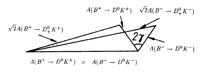
Figure 25: Triangle relations among $B^{\pm}\to DK^{\pm}$ decay amplitudes.

Combining all these considerations, we conclude that the triangle relations (8.129) and (8.130), which are depicted in fig. 25, can be used to extract $\gamma$ by measuring only the rates of the corresponding six processes. This approach was proposed by Gronau and Wyler in [293]. It is theoretically clean and suffers from no hadronic uncertainties. Unfortunately the triangles are expected to be very squashed ones since $B^{+}\to D^{0}K^{+}$ is both colour- and CKM-suppressed with respect to $B^{+}\to\overline{D^{0}}K^{+}$:

$$\frac{|A(B^{+}\to D^{0}K^{+})|}{|A(B^{+}\to\overline{D^{0}}K^{+})|}=R_{b}\,\frac{|a|}{|A|}\approx 0.36\,\frac{a_{2}}{a_{1}}\approx 0.08.$$ (8.134)

Here $a_{1}$, $a_{2}$ are the usual phenomenological colour-factors [252, 253] satisfying $a_{2}/a_{1}=0.26\pm 0.05\pm 0.09$ [254]. Using the $SU(3)$ flavour symmetry, the corresponding branching ratios can be estimated from the measured value $(5.3\pm 0.5)\cdot 10^{-3}$ [60] of $Br(B^{+}\to\overline{D^{0}}\pi^{+})$ to be $Br(B^{+}\to\overline{D^{0}}K^{+})\approx 4\cdot 10^{-4}$ and $Br(B^{+}\to D^{0}K^{+})\approx 2\cdot 10^{-6}$. While the former branching ratio can be measured using conventional methods, the latter one suffers from considerable experimental problems. The point is that if $Br(B^{+}\to D^{0}K^{+})$ is measured using hadronic tags of the $D^{0}$, e.g. $D^{0}\to K^{-}\pi^{+}$, one has to deal with large interference effects of ${\cal O}(1)$ with the $\overline{D^{0}}$ channel, e.g. $B^{+}\to K^{+}\overline{D^{0}}[\to K^{-}\pi^{+}]$, as has been pointed out recently [295]. That problem is not present in the semi-leptonic decay $D^{0}\to l^{+}\nu_{l}X_{s}$. However, here one has to deal with huge backgrounds, e.g. from $B^{+}\to l^{+}\nu_{l}X_{c}$, which are ${\cal O}(10^{-6})$ larger and may be difficult to become under control [295]. Another problem is related to the CP eigenstate of the neutral $D$ system. It is detected through $D^{0}_{+}\to\pi^{+}\pi^{-},K^{+}K^{-},\ldots$ and is experimentally challenging since the corresponding $Br\times$(detection efficiency) is expected to be at most of ${\cal O}(1\%)$. Therefore the Gronau-Wyler method [293] will unfortunately be very difficult from the experimental point of view.

A variant of the clean determination of $\gamma$ discussed above was proposed by Dunietz in [294] and uses the decays $B^{0}_{d}\to D^{0}_{+}K^{\ast 0}$, $B^{0}_{d}\to\overline{D^{0}}K^{\ast 0}$, $B^{0}_{d}\to D^{0}K^{\ast 0}$ and their charge-conjugates. Since these modes are “self-tagging” through $K^{\ast 0}\to K^{+}\pi^{-}$, no time-dependent measurements are needed in this method although neutral $B_{d}$ decays are involved. Compared to the Gronau-Wyler approach [293], both $B^{0}_{d}\to\overline{D^{0}}K^{\ast 0}$ and $B^{0}_{d}\to D^{0}K^{\ast 0}$ are colour-suppressed, i.e.

$$\frac{|A(B^{0}_{d}\to D^{0}K^{\ast 0})|}{|A(B^{0}_{d}\to\overline{D^{0}}K^{\ast 0})|}\approx R_{b}\,\frac{a_{2}}{a_{2}}\approx 0.36.$$ (8.135)

Consequently the amplitude triangles are probably not as as squashed as in the $B^{\pm}\to DK^{\pm}$ case. The corresponding branching ratios are expected to be of ${\cal O}(10^{-5})$. Unfortunately one has also to deal with the difficulties of detecting the neutral $D$-meson CP eigenstate $D^{0}_{+}$.

That problem is not present in the approach to extract $\gamma$ proposed in an interesting recent paper [295], where the decay chains $B^{-}\to K^{-}D^{0}\,[\to f]$ and $B^{-}\to K^{-}\overline{D^{0}}\,[\to f]$ with $f$ denoting a doubly Cabibbo-suppressed (Cabibbo-favoured) non-CP mode of $D^{0}$ ($\overline{D^{0}}$) were considered. Examples of such decays are $f\in\{K^{+}\pi^{-},K\pi\pi\}$. In contrast to $B^{-}\to D^{0}_{+}K^{-}$ discussed above, here both contributing decay amplitudes should be of comparable size and potentially large CP-violating asymmetries proportional to the rate difference $Br(B^{+}\to K^{+}[\overline{f}])-Br(B^{-}\to K^{-}[f])$ are expected. Since several hadronic final states $f$ of neutral $D$ mesons with different strong phases can be considered, the difficult to measure branching ratio $Br(B^{+}\to K^{+}D^{0})$ is not required in order to extract $\gamma$. Rather both $Br(B^{+}\to K^{+}D^{0})/Br(B^{+}\to K^{+}\overline{D^{0}})$ and $\gamma$ can in principle be determined. To this end an accurate measurement of the relevant $D$ branching ratios is also very desirable. For the details of this approach the reader is referred to [295].

8.8.2 $SU(3)$ Amplitude Relations

In a series of interesting papers [277, 296], Gronau, Hernández, London and Rosner (GHLR) pointed out that the $SU(3)$ flavour symmetry of strong interactions [297] – which appeared already several times in this review – can be combined with certain plausible dynamical assumptions, e.g. neglect of annihilation topologies, to derive amplitude relations among $B$ decays into $\pi\pi$, $\pi K$ and $K\overline{K}$ final states. These relations may allow determinations both of weak phases of the CKM matrix and of strong final state interaction phases by measuring only the corresponding branching ratios.

In order to illustrate this approach, let us describe briefly the “state of the art” one had about 3 years ago. At that time it was assumed that EW penguins should play a very minor role in non-leptonic $B$ decays and consequently their contributions were not taken into account. Within that approximation, which will be analyzed very carefully in section 9, the decay amplitudes for $B\to\{\pi\pi,\pi K,K\overline{K}\}$ transitions can be represented in the limit of an exact $SU(3)$ flavour symmetry in terms of five reduced matrix elements. This decomposition can also be performed in terms of diagrams. At the quark-level one finds six different topologies of Feynman diagrams contributing to $B\to\{\pi\pi,\pi K,K\overline{K}\}$ that show up in the corresponding decay amplitudes only as five independent linear combinations [277, 296]. In contrast to the classification of non-leptonic $B$ decays performed in Subsection 8.2, these six topologies of Feynman diagrams include also three non-spectator diagrams, i.e. annihilation processes, where the decaying $b$-quark interacts with its partner anti-quark in the $B$-meson. However, due to dynamical reasons, these three contributions are expected to be suppressed relative to the others and hence should play a very minor role. Consequently, neglecting these diagrams, $6-3=3$ topologies of Feynman diagrams suffice to represent the transition amplitudes of $B$ decays into $\pi\pi$, $\pi K$ and $K\overline{K}$ final states. To be specific, these diagrams describe “colour-allowed” and “colour-suppressed” current-current processes $T$ $(T^{\prime})$ and $C$ $(C^{\prime})$, respectively, and QCD penguins $P$ $(P^{\prime})$. As in [277, 296] and in 8.6.2, an unprimed amplitude denotes strangeness-preserving decays, whereas a primed amplitude stands for strangeness-changing transitions. Note that the colour-suppressed topologies $C$ and $C^{\prime}$ involve the colour-suppression factor $a_{2}\approx 0.2$ [252]-[254].

Let us consider the decays $B^{+}\to\{\pi^{+}\pi^{0},\pi^{+}K^{0},\pi^{0}K^{+}\}$, i.e. the “original” GRL method [277], as an example. Neglecting both EW penguins, which will be discussed later, and the dynamically suppressed non-spectator contributions mentioned above, the decay amplitudes of these modes can be expressed as

$$\begin{array}[]{rcl}\sqrt{2}\,A(B^{+}\to\pi^{+}\pi^{0})&=&-\left(T+C\right)\\ A(B^{+}\to\pi^{+}K^{0})&=&P^{\prime}\\ \sqrt{2}\,A(B^{+}\to\pi^{0}K^{+})&=&-\left(T^{\prime}+C^{\prime}+P^{\prime}\right)\end{array}$$ (8.136)

with

$$T=|T|\,e^{i\gamma}\,e^{i\delta_{T}},\quad C=|C|\,e^{i\gamma}\,e^{i\delta_{C}}.$$ (8.137)

Here $\delta_{T}$ and $\delta_{C}$ denote CP-conserving strong phases. Using the $SU(3)$ flavour symmetry, the strangeness-changing amplitudes $T^{\prime}$ and $C^{\prime}$ can be obtained easily from the strangeness-preserving ones through

$$\frac{T^{\prime}}{T}\approx\frac{C^{\prime}}{C}\approx\lambda\frac{F_{K}}{F_{\pi}}\equiv r_{u},$$ (8.138)

where $F_{K}$ and $F_{\pi}$ take into account factorizable $SU(3)$-breaking corrections as in (8.103). The structures of the $\bar{b}\to\bar{d}$ and $\bar{b}\to\bar{s}$ QCD penguin amplitudes $P$ and $P^{\prime}$ corresponding to $P^{(d)}$ and $P^{(s)}$ (see (8.76) and (8.77)), respectively, have been discussed in 8.5.4. It is an easy exercise to combine the decay amplitudes given in (8.136) appropriately to derive the relations

$$\sqrt{2}\,A(B^{+}\to\pi^{0}K^{+})+A(B^{+}\to\pi^{+}K^{0}) = r_{u}\sqrt{2}\,A(B^{+}\to\pi^{+}\pi^{0})$$ (8.139)

$$\sqrt{2}\,A(B^{-}\to\pi^{0}K^{-})+A(B^{-}\to\pi^{-}\overline{K^{0}}) = r_{u}\sqrt{2}\,A(B^{-}\to\pi^{-}\pi^{0}),$$ (8.140)

which can be represented as two triangles in the complex plane. If one measures the rates of the corresponding six decays, these triangles can easily be constructed. Their relative orientation is fixed through $A(B^{+}\to\pi^{+}K^{0})=A(B^{-}\to\pi^{-}\overline{K^{0}})$, which is due to the fact that there is no non-trivial CP-violating weak phase present in the $\bar{b}\to\bar{s}$ QCD penguin amplitude governing $B^{+}\to\pi^{+}K^{0}$ as we have seen in 8.5.4. Taking into account moreover (8.137), we conclude that these triangles should allow a determination of $\gamma$ as can be seen in fig. 26. From the geometrical point of view, that GRL approach [277] is very similar to the $B^{\pm}\to DK^{\pm}$ construction [293] shown in fig. 25. Furthermore it involves also only charged $B$ decays and therefore neither time-dependent measurements nor tagging are required. In comparison with the Gronau-Wyler method [293], at first sight the major advantage of the GRL strategy seems to be that all branching ratios are expected to be of the same order of magnitude ${\cal O}(10^{-5})$, i.e. the corresponding triangles are not squashed ones, and that the difficult to measure CP eigenstate $D^{0}_{+}$ and $Br(B^{+}\to D^{0}K^{+})$ are not required. The decay $B^{+}\to\pi^{+}K^{0}$ has been measured already by the CLEO collaboration with a branching ratio $\left(2.3^{+1.1+0.2}_{-1.0-0.2}\pm 0.2\right)\cdot 10^{-5}$, while presently only the upper bounds $Br(B^{+}\to K^{+}\pi^{0})<1.6\cdot 10^{-5}$ and $Br(B^{+}\to\pi^{+}\pi^{0})<2.0\cdot 10^{-5}$ are available for the other decays [266].

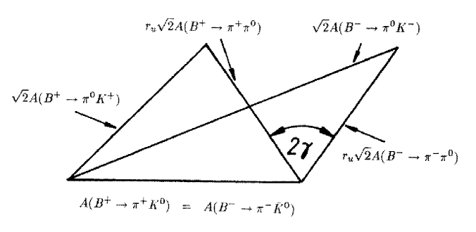
Figure 26: Naive $SU(3)$ triangle relations among $B^{+}\to\{\pi^{+}\pi^{0},\pi^{+}K^{0},\pi^{0}K^{+}\}$ and charge-conjugate decay amplitudes neglecting EW penguin contributions.

However, things are unfortunately not that simple and – despite of its attractiveness – the general GHLR approach [277, 296] to extract CKM phases from $SU(3)$ amplitude relations suffers from theoretical limitations. The most obvious limitation is of course related to the fact that the relations are not, as e.g. (8.129) or (8.130), valid exactly but suffer from $SU(3)$-breaking corrections [298]. While factorizable $SU(3)$-breaking can be included straightforwardly through certain meson decay constants or form factors, non-factorizable $SU(3)$-breaking corrections cannot be described in a reliable quantitative way at present. Another limitation is related to $\bar{b}\to\bar{d}$ QCD penguin topologies with internal up- and charm-quark exchanges which may affect the simple relation (8.81) between $\beta$ and the $\bar{b}\to\bar{d}$ QCD penguin amplitude $P$ significantly as we have seen in 8.5.4. Consequently these contributions may preclude reliable extractions of $\beta$ using $SU(3)$ amplitude relations and the assumption that $\bar{b}\to\bar{d}$ QCD penguin amplitudes are dominated by internal top-quark exchanges (see also 8.5.6) [264]. Remarkably also EW penguins [238, 299, 300], which we have neglected in our discussion of $SU(3)$ amplitude relations so far, have a very important impact on some $SU(3)$ constructions, in particular on the GRL method [277] of determining $\gamma$. As we will see in subsection 9.3, this approach is even spoiled by these contributions [301, 302]. However, there are other – generally more involved – $SU(3)$ methods that are not affected by EW penguins [302]-[305]. Interestingly it is in principle also possible to shed light on the physics of these operators by using $SU(3)$ amplitude relations [305, 306]. This issue has been one of the “hot topics” in $B$ physics over the last few years and will be the subject of the following section.

8.9 Summary and Outlook

The $B$-meson system provides a very fertile ground for studying CP violation and extracting CKM phases. In this respect neutral $B_{q}$ decays ($q\in\{d,s\}$) are particularly promising. The point is that “mixing-induced” CP-violating asymmetries are closely related to angles of the unitarity triangle in some cases. For example, the “gold-plated” decay $B_{d}\to J/\psi\,K_{\mbox{{\scriptsize S}}}$ allows an extraction of $\sin(2\beta)$ to excellent accuracy because of its particular decay structure, and $B_{d}\to\pi^{+}\pi^{-}$ probes $\sin(2\alpha)$. However, hadronic uncertainties arising from QCD penguins preclude a theoretical clean determination of $\sin(2\alpha)$ by measuring only ${\cal A}_{\mbox{{\scriptsize CP}}}^{\mbox{{\scriptsize mix-ind}}}(B_{d}\to\pi^{+}\pi^{-})$. Consequently more involved strategies are required to extract $\alpha$. Such methods are fortunately already available and certainly time will tell which of them is most promising from an experimental point of view.

In the case of $B_{s}\to\rho^{0}K_{\mbox{{\scriptsize S}}}$, which appeared frequently in the literature as a tool to determine $\gamma$, penguin contributions are expected to lead to serious problems so that a meaningful extraction of $\gamma$ from this mode should not be possible. There are, however, other $B_{s}$ decays that may allow determinations of this angle, in some cases even in a clean way. Unfortunately $B^{0}_{s}-\overline{B^{0}_{s}}$ oscillations may be too fast to be resolved with present vertex technology so that these strategies are experimentally very challenging.

An alternative route to extract CKM phases from $B_{s}$ decays and to explore CP violation in these modes may be provided by the width difference of the $B_{s}$ system that is expected to be sizable. Interestingly the rapid oscillatory $\Delta M_{s}t$ terms cancel in untagged $B_{s}$ data samples that depend therefore only on two different exponents $e^{-\Gamma_{L}^{(s)}t}$ and $e^{-\Gamma_{H}^{(s)}t}$. Several strategies to extract $\gamma$ and the Wolfenstein parameter $\eta$ from untagged $B_{s}$ decays have been proposed recently. Here time-dependent angular distributions for $B_{s}$ decays into admixtures of CP eigenstates and exclusive channels that are caused by $\bar{b}\to\bar{u}c\bar{s}$ ($b\to c\bar{u}s$) quark-level transitions play a key role. Such untagged methods are obviously much more promising in respect of efficiency, acceptance and purity than tagged ones. However, their feasibility depends crucially on $\Delta\Gamma_{s}$ and it is not clear at present whether it will turn out to be large enough.

Theoretical analyses of CP violation in charged $B$ decays are usually very technical and suffer in general from large hadronic uncertainties. Consequently CP-violating asymmetries in charged $B$ decays are mainly interesting in view of excluding “superweak” models of CP violation in an unambiguous way. Nevertheless, if one combines branching ratios of charged $B$ decays in a clever way, they may allow determinations of angles of the unitarity triangle, in some cases even without hadronic uncertainties. To this end certain relations among decay amplitudes are used. The prototype of this approach are $B\to DK$ amplitude triangles that allow a clean determination of $\gamma$. Unfortunately one has to deal with experimental problems in that strategy of fixing this angle. Whereas the $B\to DK$ triangle relations are valid exactly, one may also use the $SU(3)$ flavour symmetry of strong interactions with certain plausible dynamical assumptions to derive approximate relations among non-leptonic $B\to\{\pi\pi,\pi K,K\overline{K}\}$ decay amplitudes which may allow extractions of CKM phases and strong final state interaction phases by measuring only the corresponding branching ratios. This approach has been very popular over the recent years. It suffers, however, from limitations due to non-factorizable $SU(3)$-breaking, QCD penguins with internal up- and charm-quark exchanges and also EW penguins. A detailed discussion of the effects introduced through the latter operators is the subject of the following section.

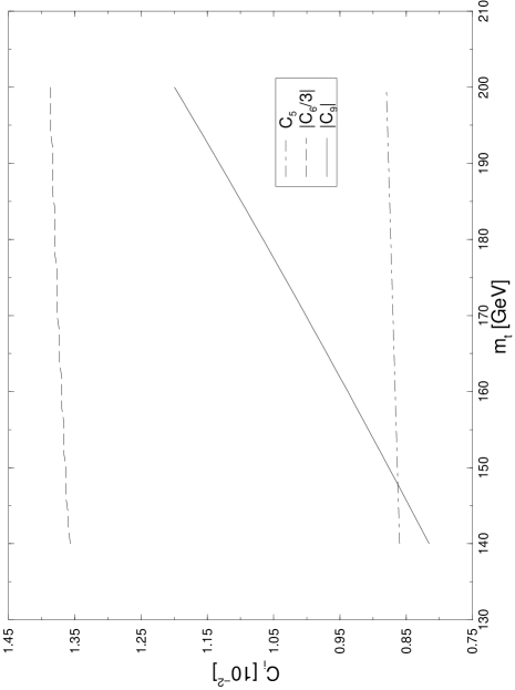
Figure 27: Dependence of Wilson coefficients $C_{5}$, $C_{6}$ and $C_{9}$ on the top-quark mass $m_{\rm t}$.

9 The Role of EW Penguins in Non-leptonic $B$ Decays and Strategies for Extracting CKM Phases

9.1 Preliminary Remarks

Since the ratio $\alpha/\alpha_{s}={\cal O}(10^{-2})$ of the QED and QCD couplings is very small, one would expect that EW penguins should only play a minor role in comparison with QCD penguins. That would indeed be the case if the top-quark was not “heavy”. However, the Wilson coefficient of one EW penguin operator – the operator $Q_{9}$ specified in (8.7) – increases strongly with the top-quark mass and becomes comparable in magnitude to Wilson coefficients of QCD penguin operators as can be seen in fig. 27. Consequently interesting EW penguin effects may arise from this feature in certain non-leptonic $B$ decays because of the large top-quark mass. As we have stressed in 4.5.1, the parameter $m_{t}$ used in NLO analyses of non-leptonic weak decays is not equal to the measured “pole” mass but refers to the running top-quark current-mass normalized at the scale $\mu=m_{t}$, i.e. $\overline{m}_{t}(m_{t})$. Before we shall investigate the role of EW penguins in methods for extracting angles of the unitarity triangle in subsection 9.3, let us have a closer look at a few non-leptonic $B$ decays that are affected significantly by EW penguin operators. These modes are listed in table 28.

$$\begin{array}[]{|c|c|c|c|}\hline\cr\mbox{Quark-Decay}&\mbox{Exclusive Decay}&\mbox{Discussed in}&\mbox{EW Penguin Contributions}\\ \hline\cr\hline\cr\bar{b}\to\bar{s}d\bar{d}&B^{+}\to\pi^{+}K^{\ast 0}&\ref{BKphi}&\mbox{negligible}\\ \hline\cr\bar{b}\to\bar{s}s\bar{s}&B^{+}\to K^{+}\phi&\ref{BKphi}&\mbox{sizable}\\ \hline\cr\bar{b}\to\bar{d}s\bar{s}&B^{+}\to\pi^{+}\phi&\ref{Bpiphi}&\mbox{dominant}\\ \hline\cr\bar{b}\to\bar{s}(u\bar{u},d\bar{d})&B_{s}\to\pi^{0}\phi&\ref{Bspi0phi}&\mbox{dominant}\\ \hline\cr\end{array}$$

Table 28: EWP effects in some non-leptonic $B$ decays. The theoretical most reliable analysis is possible in $B_{s}\to\pi^{0}\phi$ because of the isospin symmetry of strong interactions.

9.2 EW Penguin Effects in Non-leptonic $B$ Decays

The EW penguin effects discussed in this subsection were pointed out first in [238, 299, 300]. Meanwhile they were confirmed by several other authors [260, 302], [307]-[309].

Figure 28: The dependence of the ratio $R\propto Br(B^{+}\to K^{+}\phi)/Br(B^{+}\to\pi^{+}K^{\ast 0})$ on $m_{t}$.

9.2.1 EW Penguin Effects in $B^{+}\to K^{+}\phi$ and $B^{+}\to\pi^{+}K^{\ast 0}$

The channels $B^{+}\to K^{+}\phi$ and $B^{+}\to\pi^{+}K^{\ast 0}$ originating from the penguin-induced $\bar{b}$-quark decays $\bar{b}\to\bar{s}s\bar{s}$ and $\bar{b}\to\bar{s}d\bar{d}$, respectively, are very similar from a QCD point of view, i.e. as far as their QCD penguin contributions are concerned. This feature is obvious if one draws the corresponding Feynman diagrams which is an easy exercise. However, an important difference arises in respect of EW penguin contributions. We have to deal both with small colour-suppressed and sizable colour-allowed EW penguin diagrams. Whereas the former contributions are again very similar for $B^{+}\to K^{+}\phi$ and $B^{+}\to\pi^{+}K^{\ast 0}$, the colour-allowed EW penguin contributions are absent in the $B^{+}\to\pi^{+}K^{\ast 0}$ case and contribute only to $B^{+}\to K^{+}\phi$. Consequently significant EW penguin effects are expected in the mode $B^{+}\to K^{+}\phi$, while these effects should be negligible in the decay $B^{+}\to\pi^{+}K^{\ast 0}$ [238].

This rather qualitative kind of reasoning is in agreement with the results of certain model calculations [238, 307], where appropriate NLO low energy effective Hamiltonians were applied in combination with the “factorization” hypothesis [285, 286]. By factorization one means in this context that the hadronic matrix elements of the relevant four-quark operators appearing in (8.4) are factorized into the product of hadronic matrix elements of two quark-currents that are described by a set of form factors. Usually the model proposed by Bauer, Stech and Wirbel (BSW) [252] is used for these form factors and was also applied in [238, 307]. In contrast to colour-allowed current-current processes, where “factorization” may work reasonably well [287], this assumption is questionable for penguin processes which are classical examples of non-factorizable diagrams. Nevertheless this approach may give us a feeling for the expected orders of magnitudes. Unfortunately a more reliable analytical way of dealing with non-leptonic $B$ decays is not available at present.

The corresponding calculations are quite complicated and a discussion of their technicalities is beyond this review. Let us therefore just briefly discuss the main results. The model calculations indicate that EW penguins lead to a reduction of $Br(B^{+}\to K^{+}\phi)$ by ${\cal O}(30\%)$ for $m_{t}={\cal O}(170\,\mbox{GeV})$, while these effects are below $2\%$ in the case of $Br(B^{+}\to\pi^{+}K^{\ast 0})$. As in fig. 24, the branching ratios, which are both of ${\cal O}(10^{-5})$, depend strongly on $k^{2}$, the four-momentum of the gluons and photons appearing in the corresponding time-like penguin diagrams. This “unphysical” $k^{2}$-dependence is due to the use of the above mentioned model [269]. In order to reduce this dependence as well as other hadronic uncertainties, the ratio [238]

$$R\equiv\left[\frac{F_{K^{\ast}}F_{B\pi}(M_{K^{\ast}}^{2};1^{-})}{F_{\phi}F_{BK}(M_{\phi}^{2};1^{-})}\right]^{2}\left[\frac{\Phi(M_{\pi}/M_{B},M_{K^{\ast}}/M_{B})}{\Phi(M_{K}/M_{B},M_{\phi}/M_{B})}\right]^{3}$$ (9.1)

$$\times\left[\frac{Br(B^{+}\to K^{+}\phi)}{Br(B^{+}\to\pi^{+}K^{\ast 0})}\right]\approx 0.5\times\left[\frac{Br(B^{+}\to K^{+}\phi)}{Br(B^{+}\to\pi^{+}K^{\ast 0})}\right]$$

turns out to be very useful. Here $F_{V}$ are meson decay constants, $F_{PP^{\prime}}$ are quark-current form factors and $\Phi(x,y)$ is the usual two-body phase space function. Although $R$ is affected in almost the same way by EW penguins as the branching ratio $Br(B^{+}\to K^{+}\phi)$, it suffers much less from hadronic uncertainties, is very stable against variations both of the momentum transfer $k^{2}/m_{b}^{2}$ and of the QCD scale parameter $\Lambda_{\overline{\mbox{{\scriptsize MS}}}}$, and does not depend on CKM factors if the ${\cal O}(\lambda^{2})$ terms in (8.75) are neglected. These terms play a minor role and may lead to tiny direct CP-violating asymmetries of ${\cal O}(1\%)$. One should keep in mind, however, that $Br(B^{+}\to K^{+}\phi)$ and $Br(B^{+}\to\pi^{+}K^{\ast 0})$ could receive quite different contributions in principle if “factorization” does not hold. Therefore $R$ could be affected by such unknown corrections.

The effects of EW penguins can be seen nicely in fig. 28, where the top-quark mass dependence of $R$ is shown. For details of the calculation of these curves the reader is referred to [8, 238]. Whereas the dashed line corresponds to the case where only QCD penguins are included, the solid line describes the calculation taking into account both QCD and EW penguin operators.

There are not only some non-leptonic $B$ decays that are affected significantly by EW penguins. There are even a few channels where the corresponding operators may play the dominant role as we will see in the remainder of this subsection.

9.2.2 EW Penguin Effects in $B^{+}\to\pi^{+}\phi$

In respect of EW penguin effects, the mode $B^{+}\to\pi^{+}\phi$ is also quite interesting [299]. Within the spectator model, it originates from the penguin-induced $\bar{b}$-quark decay $\bar{b}\to\bar{d}s\bar{s}$, where the $s\bar{s}$ pair hadronizes into the $\phi$-meson which is present in a colour-singlet state. The $s$- and $\bar{s}$-quarks emerging from the gluons of the usual QCD penguin diagrams form, however, a colour-octet state and consequently cannot build up that $\phi$-meson (see also 8.5.2). Thus, using both an appropriate NLO low energy effective Hamiltonian and the BSW model in combination with the factorization assumption to estimate the relevant hadronic matrix elements of the QCD penguin operators, one finds a very small branching ratio $Br\left.(B^{+}\to\pi^{+}\phi)\right|_{\mbox{{\scriptsize QCD}}}={\cal O}(10^{-10})$. The non-vanishing result is due to the renormalization group evolution from $\mu={\cal O}(M_{W})$ down to $\mu={\cal O}(m_{b})$. Neglecting this evolution would give a vanishing branching ratio because of the colour-arguments given above. Since these arguments do not apply to EW penguins, their contributions are expected to become important [299]. In fact, taking into account also these operators gives a branching ratio $Br\left.(B^{+}\to\pi^{+}\phi)\right|_{\mbox{{\scriptsize QCD+EW}}}={\cal O}(10^{-8})$ for $m_{t}={\cal O}(170\,\mbox{GeV})$ that increases strongly with the top-quark mass. Unfortunately the enhancement by a factor of ${\cal O}(10^{2})$ through EW penguins is not strong enough to make the decay $B^{+}\to\pi^{+}\phi$ measurable in the foreseeable future.

The colour-arguments for the QCD penguins may be affected by additional soft gluon exchanges which are not under quantitative control at present. These contributions would show up as non-factorizable contributions to the hadronic matrix elements of the penguin operators which were neglected in [299]. Nevertheless there is no doubt that EW penguins play a very important – probably even dominant – role in the decay $B^{+}\to\pi^{+}\phi$ and related modes like $B^{+}\to\rho^{+}\phi$.

9.2.3 EW Penguin Effects in $B_{s}\to\pi^{0}\phi$

The theoretical situation arising in the decay $B_{s}^{0}\to\pi^{0}\phi$ caused by $\bar{b}\to\bar{s}\,(u\bar{u},d\bar{d})$ quark-level transitions is much more favourable than in the channels discussed previously because of the $SU(2)$ isospin symmetry of strong interactions. Let us therefore be more detailed in the presentation of that transition which is expected to be dominated by EW penguins [300]. In contrast to the decays discussed in 9.2.1 and 9.2.2, it receives not only penguin but also current-current operator contributions at the tree level. The final state is an eigenstate of the CP operator with eigenvalue +1 and has strong isospin quantum numbers $(I,I_{3})=(1,0)$, whereas the initial state is an isospin singlet. Thus we have to deal with a $\Delta I=1$ transition.

Looking at the operator basis given in (8.5)-(8.7), we observe that the current-current operators $Q^{us}_{1,2}$ and the EW penguin operators can lead to final states both with isospin $I=0$ and $I=1$, whereas the QCD penguin operators give only final states with $I=0$. Therefore the $\Delta I=1$ transition $B_{s}\to\pi^{0}\phi$ receives no QCD penguin contributions and arises purely from the current-current operators $Q^{us}_{1,2}$ and the EW penguin operators. For the same reason, QCD penguin matrix elements of the current-current operators $Q_{2}^{us}$ and $Q_{2}^{cs}$ with up- and charm-quarks running as virtual particles in the loops, respectively, do not contribute to that decay. Consequently, using in addition the unitarity of the CKM matrix and applying the modified Wolfenstein parametrization (8.1) yielding

$$V_{us}^{\ast}V_{ub}=\lambda|V_{ub}|\,e^{-i\gamma},\quad V_{ts}^{\ast}V_{tb}=-|V_{ts}|=-|V_{cb}|(1+{\cal O}(\lambda^{2})),$$ (9.2)

the hadronic matrix element of the Hamiltonian (8.4) can be expressed as

$$\Bigl{\langle}\pi^{0}\phi\Bigl{|}{\cal H}_{\mbox{{\scriptsize eff}}}(\Delta B=-1)\Bigr{|}\overline{B^{0}_{s}}\Bigr{\rangle}=\frac{G_{\mbox{{\scriptsize F}}}}{\sqrt{2}}\,|V_{ts}|$$

$$\times\left[\lambda^{2}R_{b}\,e^{-i\gamma}\sum\limits_{k=1}^{2}\Bigl{\langle}\pi^{0}\phi\Bigl{|}Q_{k}^{us}(\mu)\Bigr{|}\overline{B^{0}_{s}}\Bigr{\rangle}C_{k}(\mu)+\sum\limits_{k=7}^{10}\Bigl{\langle}\pi^{0}\phi\Bigl{|}Q_{k}^{s}(\mu)\Bigr{|}\overline{B^{0}_{s}}\Bigr{\rangle}C_{k}(\mu)\right],$$

where the correction of ${\cal O}(\lambda^{2})$ in (9.2) has been omitted.

Neglecting EW penguin operators for a moment and applying the formalism developed in 8.4.2, we would find ${\cal A}_{\mbox{{\scriptsize CP}}}^{\mbox{{\scriptsize mix-ind}}}(B_{s}\to\pi^{0}\phi)=\sin(2\gamma)$. The approximation of neglecting EW penguin operator contributions to $B_{s}\to\pi^{0}\phi$ is, however, very bad since the current-current amplitude $A_{\mbox{{\scriptsize CC}}}$ is suppressed relative to the EW penguin part $A_{\mbox{{\scriptsize EW}}}$ by the CKM factor $\lambda^{2}R_{b}\approx 0.02$. Moreover the current-current operator contribution is colour-suppressed by $a_{2}\approx 0.2$. On the other hand, in the presence of a heavy top-quark, the Wilson coefficient of the dominant EW penguin operator $Q_{9}^{s}$ contributing to $B_{s}\to\pi^{0}\phi$ in colour-allowed form is of ${\cal O}(10^{-2})$ (see fig. 27). Therefore we expect $|A_{\mbox{{\scriptsize EW}}}|/|A_{\mbox{{\scriptsize CC}}}|={\cal O}(10^{-2}/(0.02\cdot 0.2))={\cal O}(2.5)$ and conclude that EW penguins have not only to be taken into account in an analysis of $B_{s}\to\pi^{0}\phi$ but should even give the dominant contribution to that channel.

In order to simplify the following discussion, let us neglect the influence of QCD corrections to EW penguins for a moment. Using isospin symmetry and taking into account that $B_{s}\to\pi^{0}\phi$ is a $\Delta I=1$ transition, the correpsonding decay amplitude can be expressed as

$$\Bigl{\langle}\pi^{0}\phi\Bigl{|}{\cal H}_{\mbox{{\scriptsize eff}}}(\Delta B=-1)\Bigr{|}\overline{B^{0}_{s}}\Bigr{\rangle}=\frac{G_{\mbox{{\scriptsize F}}}}{\sqrt{2}}\,A_{\mbox{{\scriptsize CC}}}\left(e^{-i\gamma}+x\right)$$ (9.4)

with

$$x\equiv\frac{A_{\mbox{{\scriptsize EW}}}}{A_{\mbox{{\scriptsize CC}}}}\approx\frac{\alpha}{2\pi\lambda^{2}R_{b}\,a_{2}\sin^{2}\Theta_{\mbox{{\scriptsize W}}}}\bigl{[}5B_{0}(x_{t})-2C_{0}(x_{t})\bigr{]},$$ (9.5)

where the Inami-Lim functions [18] $B_{0}(x_{t})$ and $C_{0}(x_{t})$ are given in (2.24) and (2.25) and describe box diagrams and $Z$ penguins, respectively. The phenomenological colour-suppression factor $a_{2}$ takes into account that $A_{\mbox{{\scriptsize CC}}}$ is colour-suppressed. For the details of this calculation leading to (9.4) and (9.5), the reader is referred to [300].

Figure 29: Dependence of ${\cal A}_{\mbox{{\scriptsize CP}}}^{\mbox{{\scriptsize mix-ind}}}(B_{s}\to\pi^{0}\phi)$ on $\gamma$ for various values of $x$.

With the help of (9.4), the CP-violating observables of $B_{s}\to\pi^{0}\phi$ can be expressed as

$${\cal A}_{\mbox{{\scriptsize CP}}}^{\mbox{{\scriptsize dir}}}(B_{s}\to\pi^{0}\phi)=0,\quad{\cal A}_{\mbox{{\scriptsize CP}}}^{\mbox{{\scriptsize mix-ind}}}(B_{s}\to\pi^{0}\phi)=\frac{2\,(x+\cos\gamma)\sin\gamma}{x^{2}+2\,x\cos\gamma+1},$$ (9.6)

while the branching ratio $Br(B_{s}\to\pi^{0}\phi)$ takes the form

$${\cal R}\equiv\frac{Br(B_{s}\to\pi^{0}\phi)}{Br_{\mbox{{\scriptsize CC}}}(B_{s}\to\pi^{0}\phi)}=x^{2}+2\,x\cos\gamma+1,$$ (9.7)

where $Br_{\mbox{{\scriptsize CC}}}(B_{s}\to\pi^{0}\phi)={\cal O}(10^{-8})$ denotes the current-current branching ratio.

Figure 30: Dependence of $Br(B_{s}\to\pi^{0}\phi)/Br_{\mbox{{\scriptsize CC}}}(B_{s}\to\pi^{0}\phi)$ on $\gamma$ for various values of $x$.

Note that (9.5) is rather clean concerning hadronic uncertainties. This nice feature is due to the fact that we are in a position to absorb all non-perturbative $B$-parameters related to deviations from naive factorization of the hadronic matrix elements by introducing the phenomenological colour-suppression factor $a_{2}$. Concerning short-distance QCD corrections, which have been neglected so far, we have to consider only those affecting the box diagrams and $Z$ penguins contributing to $x$, since the QCD corrections to the current-current operators are incorporated effectively in $a_{2}$. The corresponding short-distance QCD corrections are small if we use $\overline{m}_{t}(m_{t})$ (see section 7). On the other hand, the QCD corrections to EW penguin operators arising from the renormalization group evolution from $\mu={\cal O}(M_{W})$ down to $\mu={\cal O}(m_{b})$ modify $x$ by only a few percent and are hence also negligibly small.

Using as an example $a_{2}=0.25$, $R_{b}=0.36$ and $m_{t}=170\,\mbox{GeV}$ yields $x\approx-3$ and confirms nicely our qualitative expectation that EW penguins should play the dominant role in $B_{s}\to\pi^{0}\phi$. Varying $a_{2}$ within $0.2\,\,\mbox{{\scriptsize$\stackrel{{\scriptstyle<}}{{\sim}}$}}\,\,a_{2}\,\,\mbox{{\scriptsize$\stackrel{{\scriptstyle<}}{{\sim}}$}}\,\,0.3$ and $R_{b}$ and $m_{t}$ within their presently allowed experimental ranges gives $-5\,\,\mbox{{\scriptsize$\stackrel{{\scriptstyle<}}{{\sim}}$}}\,\,x\,\,\mbox{{\scriptsize$\stackrel{{\scriptstyle<}}{{\sim}}$}}-2$. The EW penguin contributions lead to dramatic effects in the mixing-induced CP asymmetry as well as in the branching ratio as can be seen in Figs. 29 and 30, where the dependences of ${\cal A}_{\mbox{{\scriptsize CP}}}^{\mbox{{\scriptsize mix-ind}}}(B_{s}\to\pi^{0}\phi)$ and of the ratio ${\cal R}$ on $\gamma$ are shown for various values of $x$. The solid lines in these figures correspond to the case where EW penguins are neglected completely. In the case of ${\cal A}_{\mbox{{\scriptsize CP}}}^{\mbox{{\scriptsize mix-ind}}}(B_{s}\to\pi^{0}\phi)$ even the sign is changed through the EW penguin contributions for $\gamma<90^{\circ}$, whereas the branching ratio is enhanced by a factor of ${\cal O}(10)$ with respect to the pure current-current case. The resulting $Br(B_{s}\to\pi^{0}\phi)$ is of ${\cal O}(10^{-7})$, so that an experimental investigation of that decay – which would be interesting to explore EW penguins – will unfortunately be very difficult. Needless to say, the modes $B_{s}\to\rho^{0}\phi,\pi^{0}\eta,\rho^{0}\eta$ exhibiting a very similar dynamics should also be dominated by their EW penguin contributions [302, 308].

9.3 EW Penguin Effects in Strategies for Extracting CKM Phases

In the strategies for extracting CKM phases reviewed in section 8, EW penguins do not lead to problems wherever it has not been emphasized explicitly. That is in fact the case for most of these methods. However, the GL approach [258] to eliminate the penguin uncertainties affecting the determination of $\alpha$ from ${\cal A}_{\mbox{{\scriptsize CP}}}^{\mbox{{\scriptsize mix-ind}}}(B_{d}\to\pi^{+}\pi^{-})$ with the help of isospin relations among $B\to\pi\pi$ decays (see 8.5.3), as well as the GRL method [277] to determine $\gamma$ from $SU(3)$ amplitude relations involving $B^{+}\to\{\pi^{+}\pi^{0},\pi^{+}K^{0},\pi^{0}K^{+}\}$ and their charge-conjugates (see 8.8.2) require a careful investigation [301, 302, 306].

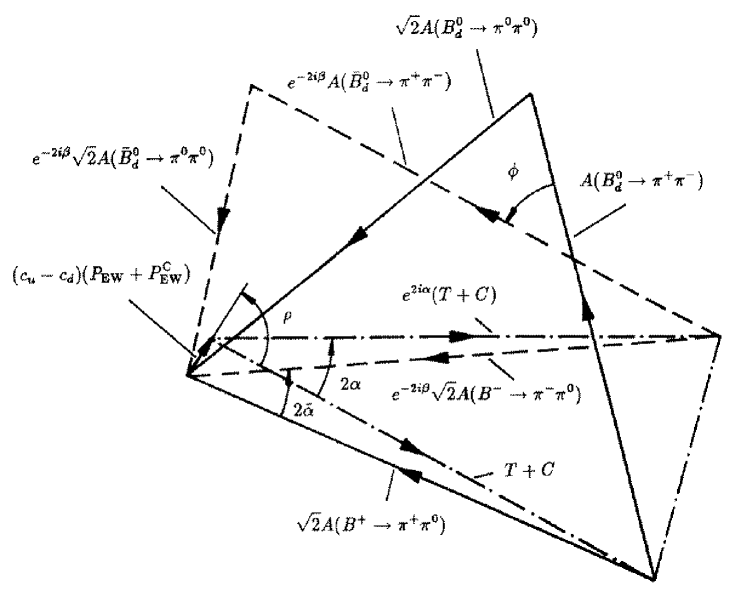
Figure 31: The determination of $\alpha$ from $B\to\pi\pi$ isospin triangles in the presence of EW penguins.

9.3.1 The GL Method of Extracting $\alpha$

If one redraws the GL construction [258] to determine $\alpha$ from $B\to\pi\pi$ isospin triangles by taking into account EW penguin contributions, one obtains the situation shown in fig. 31. This construction [306] is a bit different from the original one presented in [258], since the $A(\overline{B}\to\pi\pi)$ amplitudes have been rotated by $e^{-2i\beta}$. The angle $\phi$ fixing the relative orientation of the two isospin triangles, which are constructed by measuring only the corresponding six branching ratios, is determined from the mixing-induced CP asymmetry of $B_{d}\to\pi^{+}\pi^{-}$ with the help of the relation

$${\cal A}_{\mbox{{\scriptsize CP}}}^{\mbox{{\scriptsize mix-ind}}}(B_{d}\to\pi^{+}\pi^{-})=-\,\frac{2\,\bigl{|}A(\overline{B^{0}_{d}}\to\pi^{+}\pi^{-})\bigr{|}\bigl{|}A(B^{0}_{d}\to\pi^{+}\pi^{-})\bigr{|}}{\bigl{|}A(\overline{B^{0}_{d}}\to\pi^{+}\pi^{-})\bigr{|}^{2}+\bigl{|}A(B^{0}_{d}\to\pi^{+}\pi^{-})\bigr{|}^{2}}\,\sin\phi\,.$$ (9.8)

In fig. 31, the notation of GHLR [302] has been used, where $P_{\mbox{{\scriptsize EW}}}$ and $P_{\mbox{{\scriptsize EW}}}^{\mbox{{\scriptsize C}}}$ denote colour-allowed and colour-suppressed $\bar{b}\to\bar{d}$ EW penguin amplitudes and $c_{u}=+2/3$ and $c_{d}=-1/3$ are the electrical up- and down-type quark charges, respectively. Because of the presence of EW penguins, the construction shown in that figure does not allow the determination of the exact angle $\alpha$ of the UT. It allows only the extraction of an angle $\tilde{\alpha}$ that is related to $\alpha$ through

$$\alpha=\tilde{\alpha}+\Delta\alpha,$$ (9.9)

where $\Delta\alpha$ is given by

$$\Delta\alpha=r\,\sin\alpha\,\cos\,(\rho-\alpha)+{\cal O}(r^{2})$$ (9.10)

with

$$r\equiv\frac{\left|(c_{u}-c_{d})(P_{\mbox{{\scriptsize EW}}}+P_{\mbox{{\scriptsize EW}}}^{\mbox{{\scriptsize C}}})\right|}{|T+C|}\approx\left|\frac{P_{\mbox{{\scriptsize EW}}}}{T}\right|.$$ (9.11)

Since $r$ is expected to be of ${\cal O}(10^{-2})$ as can be shown by using a plausible hierarchy of $\bar{b}\to\bar{d}$ decay amplitudes [302], EW penguins should not lead to serious problems in the GL method. This statement can also be put on more quantitative ground. Unfortunately $\rho$ contains strong final state interaction phases and hence cannot be calculated at present. However, using $|\cos(\rho-\alpha)|\leq 1$, one may estimate the following upper bound for the uncertainty $\Delta\alpha$ [305]:

$$|\Delta\alpha|\,\,\mbox{{\scriptsize$\stackrel{{\scriptstyle<}}{{\sim}}$}}\,\,\frac{\alpha}{2\pi a_{1}\sin^{2}\Theta_{\mbox{{\scriptsize W}}}}\bigl{|}5B(x_{t})-2C(x_{t})\bigr{|}\cdot\left|\frac{V_{td}}{V_{ub}}\right|\left|\sin\alpha\right|\,.$$ (9.12)

Taking into account the present status of the CKM matrix yielding $|V_{td}|/|V_{ub}|\leq 4.6$ [95] gives $|\Delta\alpha|/|\sin\alpha|\,\,\mbox{{\scriptsize$\stackrel{{\scriptstyle<}}{{\sim}}$}}\,4^{\circ}$ for a top-quark mass $m_{t}=170\,\mbox{GeV}$ and a phenomenological colour-factor $a_{1}=1$.

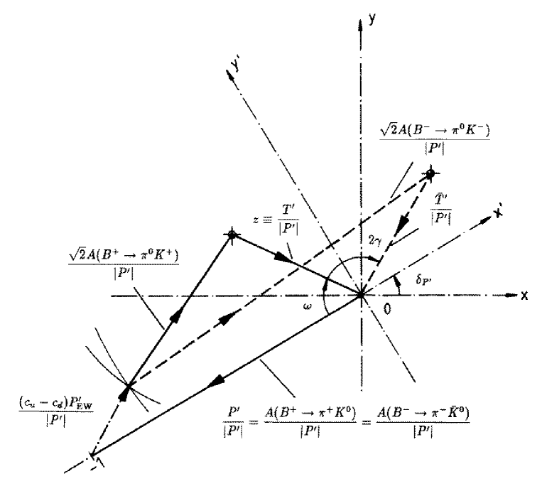
Figure 32: $SU(3)$ relations among $B^{+}\to\{\pi^{+}\pi^{0},\pi^{+}K^{0},\pi^{0}K^{+}\}$ and charge-conjugate decay amplitudes including EW penguin contributions.

9.3.2 The GRL Method of Extracting $\gamma$

In the case of the GRL strategy [277] of extracting the angle $\gamma$ from the construction shown in fig. 26, we have to deal with $\bar{b}\to\bar{s}$ modes which exhibit an interesting hierarchy of decay amplitudes that is very different from the $\bar{b}\to\bar{d}$ case [301, 302]. Since the colour-allowed current-current amplitude $T^{\prime}$ is highly CKM suppressed by $\lambda^{2}R_{b}\approx 0.02$, one expects that the QCD penguin amplitude $P^{\prime}$ plays the dominant role in this decay class and that $T^{\prime}$ and the colour-allowed EW penguin amplitude $P^{\prime}_{\mbox{{\scriptsize EW}}}$ are equally important [302]:

$$\left|\frac{T^{\prime}}{P^{\prime}}\right|={\cal O}(0.2),\quad\left|\frac{P^{\prime}_{\mbox{{\scriptsize EW}}}}{T^{\prime}}\right|={\cal O}(1)\,.$$ (9.13)

The last ratio can be estimated more quantitatively as [305]

$$\left|\frac{P^{\prime}_{\mbox{{\scriptsize EW}}}}{T^{\prime}}\right|\approx\frac{\alpha}{2\pi\lambda^{2}R_{b}\,a_{1}\sin^{2}\Theta_{\mbox{{\scriptsize W}}}}\bigl{|}5B_{0}(x_{t})-2C_{0}(x_{t})\bigr{|}\,r_{SU(3)}.$$ (9.14)

Here $r_{SU(3)}$ takes into account $SU(3)$-breaking corrections. Factorizable corrections are described by

$$\left.r_{SU(3)}\right|_{\mbox{{\scriptsize fact}}}=\frac{F_{\pi}}{F_{K}}\frac{F_{BK}(0;0^{+})}{F_{B\pi}(0;0^{+})},$$ (9.15)

where the BSW form factors [252] parametrizing the corresponding quark-current matrix elements yield $\left.r_{SU(3)}\right|_{\mbox{{\scriptsize fact}}}\approx 1$. The ratio (9.14) increases significantly with the top-quark mass. Using $m_{t}=170\,\mbox{GeV}$, $R_{b}=0.36$, $a_{1}=1$ and $r_{SU(3)}=1$ gives $|P^{\prime}_{\mbox{{\scriptsize EW}}}|/|T^{\prime}|\approx 0.8$ and confirms the expectation (9.13).

Consequently EW penguins are very important in that case and even spoil the GRL approach [277] to determine $\gamma$ as was pointed out by Deshpande and He [301]. This feature can be seen in fig. 32, where colour-suppressed EW penguin and current-current amplitudes are neglected to simplify the presentation [306]. If the EW penguin amplitude $(c_{u}-c_{d})\,P^{\prime}_{\mbox{{\scriptsize EW}}}$ were not there, this figure would correspond to fig. 26 and we would simply have to deal with two triangles in the complex plane that could be fixed by measuring only the six branching ratios corresponding to $B^{+}\to\{\pi^{+}\pi^{0},\pi^{+}K^{0},\pi^{0}K^{+}\}$ and their charge-conjugates. However, EW penguins do contribute and since the magnitude of their “unknown” amplitude $(c_{u}-c_{d})\,P^{\prime}_{\mbox{{\scriptsize EW}}}$ is of the same size as $|T^{\prime}|$, it is unfortunately not possible to determine $\gamma$ with the help of this construction. This feature led to the development of other methods using $SU(3)$ amplitude relations to extract $\gamma$ that require similarly as the GRL method only measurements of branching ratios, and to strategies to control EW penguins in a quantitative way to shed light on the physics of these FCNC processes.

9.4 $SU(3)$ Strategies for Extracting $\gamma$ that are not affected by EW Penguins

In the recent literature some solutions have been proposed to solve the problem arising from EW penguins in the GRL approach [302]-[305]. Let us have a closer look at them in this subsection.

Figure 33: Amplitude quadrangle for $B\to\pi K$ decays. The labels are explained in the text.

9.4.1 Amplitude Quadrangle for $B\to\pi K$ Decays

A quadrangle construction involving $B\to\pi K$ decay amplitudes was proposed in [302] that can be used in principle to determine $\gamma$ irrespectively of the presence of EW penguins. This construction is shown in fig. 33, where (a) corresponds to $A(B^{+}\to\pi^{+}K^{0})$, (b) to $\sqrt{2}\,A(B^{+}\to\pi^{0}K^{+})$, (c) to $\sqrt{2}\,A(B^{0}_{d}\to\pi^{0}K^{0})$, (d) to $A(B^{0}_{d}\to\pi^{-}K^{+})$ and the dashed line (e) to the decay amplitude $\sqrt{3}\,A(B_{s}^{0}\to\pi^{0}\eta)$. The dotted line (f) denotes an $I=3/2$ isospin amplitude $A_{3/2}$ that is composed of two parts and can be written as [302]

$$A_{3/2}=\bigl{|}A_{\pi K}^{\mbox{{\scriptsize T}}}\bigr{|}\,e^{i\tilde{\delta}_{T}}\,e^{i\gamma}-\bigl{|}A_{\pi K}^{\mbox{{\scriptsize EWP}}}\bigr{|}\,e^{i\tilde{\delta}_{\mbox{{\scriptsize EWP}}}}\,.$$ (9.16)

The corresponding charge-conjugate amplitude takes on the other hand the form

$$\overline{A}_{3/2}=\bigl{|}A_{\pi K}^{\mbox{{\scriptsize T}}}\bigr{|}\,e^{i\tilde{\delta}_{T}}\,e^{-i\gamma}-\bigl{|}A_{\pi K}^{\mbox{{\scriptsize EWP}}}\bigr{|}\,e^{i\tilde{\delta}_{\mbox{{\scriptsize EWP}}}}\,,$$ (9.17)

so that the EW penguin contributions cancel in the difference of (9.16) and (9.17):

$$A_{3/2}-\overline{A}_{3/2}=2\,i\,e^{i\tilde{\delta}_{T}}\,\bigl{|}A_{\pi K}^{\mbox{{\scriptsize T}}}\bigr{|}\,\sin\gamma\,.$$ (9.18)

In order to determine this amplitude difference geometrically, both the quadrangle depicted in fig. 33 and the one corresponding to the charge-conjugate processes have to be constructed by measuring the branching ratios corresponding to (a)–(e). Moreover the relative orientation of these two quadrangles in the complex plane has to be fixed. This can be done through the side (a) as no non-trivial CP-violating weak phase is present in the $\bar{b}\to\bar{s}$ penguin-induced decay $B^{+}\to\pi^{+}K^{0}$, i.e.  $A(B^{-}\to\pi^{-}\overline{K^{0}})=A(B^{+}\to\pi^{+}K^{0})$ (see 8.5.4). Since the quantity $\bigl{|}A_{\pi K}^{\mbox{{\scriptsize T}}}\bigr{|}$ corresponds to $|T^{\prime}+C^{\prime}|$, it can be determined with the help of the $SU(3)$ flavour symmetry (note (8.136) and (8.138)) by measuring the branching ratio for $B^{+}\to\pi^{+}\pi^{-}$, i.e. through $\bigl{|}A_{\pi K}^{\mbox{{\scriptsize T}}}\bigr{|}=r_{u}\,\sqrt{2}\,|A(B^{+}\to\pi^{+}\pi^{0})|$, so that both $\sin\gamma$ and the strong phase $\tilde{\delta}_{T}$ can be extracted from the amplitude difference (9.18). Unfortunately the dashed line (e) corresponds to the decay $B^{0}_{s}\to\pi^{0}\eta$ that is dominated by EW penguins [300, 308] (see 9.2.3) and is therefore expected to exhibit a branching ratio at the ${\cal O}(10^{-7})$ level. Consequently the amplitude quadrangles are rather squashed ones and this approach to determine $\gamma$ is very difficult from an experimental point of view.

Figure 34: $SU(3)$ amplitude relations involving $B^{+}\to\{\pi^{+}K^{0},\pi^{0}K^{+},\eta_{8}\,K^{+}\}$ and charge-conjugates (dashed lines). The labels are explained in the text.

9.4.2 $SU(3)$ Relations among $B^{+}\to\{\pi^{+}K^{0},\pi^{0}K^{+},\eta_{8}\,K^{+}\}$ Decay Amplitudes

Another approach to extract $\gamma$ involving the decays $B^{+}\to\{\pi^{+}K^{0},\pi^{0}K^{+},\eta_{8}\,K^{+}\}$ and their charge-conjugates was proposed by Deshpande and He in [303]. Using $SU(3)$ flavour symmetry, it is possible to derive relations among the corresponding decay amplitudes that can be represented in the complex plane as shown in fig. 34. Here the solid lines labelled (a), (b) and (c) correspond to the decay amplitudes $A(B^{+}\to\pi^{+}K^{0})$, $\sqrt{2}\,A(B^{+}\to\pi^{0}K^{+})$ and $\sqrt{6}\,A(B^{+}\to\eta_{8}\,K^{+})$, respectively, and the dashed lines represent the corresponding charge-conjugate amplitudes. Note that $A(B^{-}\to\pi^{-}\overline{K^{0}})=A(B^{+}\to\pi^{+}K^{0})$ has also been used in this construction. Similarly as in 9.4.1, the determination of $\gamma$ can be accomplished by considering the difference of a particularly useful chosen combination $A$ of decay amplitudes and its charge-conjugate $\overline{A}$, where the penguin contributions cancel:

$$A-\overline{A}=2\,\sqrt{2}\,i\,e^{i\tilde{\delta}_{T}}r_{u}\,|A(B^{+}\to\pi^{+}\pi^{0})|\,\sin\gamma\,.$$ (9.19)

Here the magnitude of the $B^{+}\to\pi^{+}\pi^{0}$ amplitude is used – as in the $B\to\pi K$ quadrangle approach [302] – to fix $|T^{\prime}+C^{\prime}|$. In fig. 34, the dotted lines (x) and (y) represent two possible solutions for this amplitude difference. The fact that this construction does not give a unique solution for $A-\overline{A}$ is a well-known characteristic feature of all geometrical constructions of this kind, i.e. one has in general to deal with several discrete ambiguities.

Compared to the method using $B\to\pi K$ quadrangles discussed in 9.4.1, the advantage of this strategy is that all branching ratios are expected to be of the same order of magnitude ${\cal O}(10^{-5})$. In particular one has not to deal with an EW penguin dominated channel with an expected branching ratio at the ${\cal O}(10^{-7})$ level. However, the accuracy of the strategy is limited by $\eta-\eta^{\prime}$ mixing, i.e. the $A(B^{\pm}\to\eta_{8}\,K^{\pm})$ amplitudes have to be determined through

$$A(B^{\pm}\to\eta_{8}\,K^{\pm})=A(B^{\pm}\to\eta\,K^{\pm})\cos\Theta+A(B^{\pm}\to\eta^{\prime}K^{\pm})\sin\Theta$$ (9.20)

with a mixing angle $\Theta\approx 20^{\circ}$, and by other $SU(3)$-breaking effects which cannot be calculated at present. A similar approach to determine $\gamma$ was proposed by Gronau and Rosner in [304], where the amplitude construction is expressed in terms of the physical $\eta$ and $\eta^{\prime}$ states. A detailed discussion of $SU(3)$ amplitude relations for $B$ decays involving $\eta$ and $\eta^{\prime}$ in light of extractions of CKM phases can be found in [310].

9.4.3 A Simple Strategy for Fixing $\gamma$ and Obtaining Insights into the World of EW Penguins

Since the geometrical constructions discussed in 9.4.1 and 9.4.2 are quite complicated and appear to be very challenging from an experimental point of view, let us consider a much simpler approach to determine $\gamma$ [305]. It uses the decays $B^{+}\to\pi^{+}K^{0}$, $B^{0}_{d}\to\pi^{-}K^{+}$ and their charge-conjugates. In the case of these transitions, EW penguins contribute only in colour-suppressed form and hence play a minor role. Neglecting these contributions and using the $SU(2)$ isospin symmetry of strong interactions – not $SU(3)$ – to relate their QCD penguin contributions (note the similarity to the example given in 8.6.2), the corresponding decay amplitudes can be written in the GHLR notation as [296]

$$A(B^{+}\to\pi^{+}K^{0}) = P^{\prime}\,=\,A(B^{-}\to\pi^{-}\overline{K^{0}})$$

$$A(B^{0}_{d}\to\pi^{-}K^{+}) = -\,(P^{\prime}+T^{\prime})$$ (9.21)

$$A(\overline{B^{0}_{d}}\to\pi^{+}K^{-}) = -\,(P^{\prime}+e^{-2i\gamma}\,T^{\prime})\,.$$

Let us note that these relations are on rather solid ground from a theoretical point of view. They can be represented in the complex plane as shown in fig. 35. Here (a) corresponds to $A(B^{+}\to\pi^{+}K^{0})=P^{\prime}=A(B^{-}\to\pi^{-}\overline{K^{0}})$, (b) to $A(B^{0}_{d}\to\pi^{-}K^{+})$, (c) to $A(\overline{B^{0}_{d}}\to\pi^{+}K^{-})$ and the dashed lines (d) and (e) to the colour-allowed current-current amplitudes $T^{\prime}$ and $e^{-2i\gamma}\,T^{\prime}$, respectively. The dotted lines (f)–(h) will be discussed in a moment. Note that these $B\to\pi K$ decays appeared already in 8.5.6. Combining their branching ratios with the observables of a time-dependent measurement of $B_{d}\to\pi^{+}\pi^{-}$, a simultaneous extraction of $\alpha$ and $\gamma$ may be possible [275]. The information provided by the $B\to\pi K$ modes can, however, also be used for a quite different approach that may finally allow the determination of EW penguin amplitudes.

Figure 35: $SU(2)$ isospin relations among $B^{+}\to\pi^{+}K^{0}$, $B^{0}_{d}\to\pi^{-}K^{+}$ and charge-conjugates. The labels are explained in the text.

In order to determine $\gamma$ from fig. 35, we have to know the length $|T^{\prime}|$ of the dashed lines (d) and (e). In fact, the situation is analogous to the extraction of $\gamma$ from (8.100) and (8.101) in 8.6.2. There we saw that $B^{+}\to\pi^{+}\pi^{0}$ provides an estimate of that quantity through (8.103) which is based on two assumptions: $SU(3)$ flavour symmetry and neglect of colour-suppressed current-current contributions to $B^{+}\to\pi^{+}\pi^{0}$. Consequently, following these lines, it is possible to obtain an estimate of $\gamma$ by measuring only $Br(B^{+}\to\pi^{+}K^{0})=Br(B^{-}\to\pi^{-}\overline{K^{0}})$, $Br(B^{0}_{d}\to\pi^{-}K^{+})$, $Br(\overline{B^{0}_{d}}\to\pi^{+}K^{-})$ and $Br(B^{+}\to\pi^{+}\pi^{0})=Br(B^{-}\to\pi^{-}\pi^{0})$. Note that the neutral $B_{d}$ decays are “self-tagging” modes so that no time-dependent measurements are needed and that this estimate of $\gamma$ is very similar to the “original” GRL approach [277] shown in fig. 26 that is unfortunately spoiled by EW penguins. Needless to say, this strategy is very simple from a geometrical point of view – just triangle constructions – and very promising from an experimental point of view since all branching ratios are of the same order of magnitude ${\cal O}(10^{-5})$. Moreover no experimentally difficult CP eigenstate of the neutral $D$ system is required as in 8.8.1.

Let us emphasize that the “weak” point of this approach – and of the one using untagged $B_{s}$ decays discussed in 8.6.2 – is the relation (8.103) to estimate $|T^{\prime}|$. Therefore this “estimate” of $\gamma$ may well turn into a solid “determination” if it should become possible to fix the magnitude of the colour-allowed current-current amplitude contributing to $B^{0}_{d}\to\pi^{-}K^{+}$ in a more reliable way. Another possibility of fixing $|T^{\prime}|$ is of course the factorization hypothesis which may work reasonably well for that colour-allowed amplitude [287] and could be used as some kind of cross-check for (8.103). Maybe the “final” result for $|T^{\prime}|$ will come from lattice gauge theory one day.

Interestingly the construction shown in fig. 35 provides even more information if one takes into account the amplitude relations

$$\sqrt{2}\,A(B^{+}\to\pi^{0}K^{+}) \approx -\,\left[P^{\prime}+T^{\prime}+(c_{u}-c_{d})P_{\mbox{{\scriptsize EW}}}^{\prime}\right]$$ (9.22)

$$\sqrt{2}\,A(B^{-}\to\pi^{0}K^{-}) \approx -\,\left[P^{\prime}+e^{-2i\gamma}\,T^{\prime}+(c_{u}-c_{d})P_{\mbox{{\scriptsize EW}}}^{\prime}\right],$$ (9.23)

where colour-suppressed current-current and EW penguin amplitudes have been neglected. Consequently, the dotted lines (f) and (g) corresponding to $\sqrt{2}\,A(B^{+}\to\pi^{0}K^{+})$ and $\sqrt{2}\,A(B^{-}\to\pi^{0}K^{-})$, respectively, allow a determination of the dotted line (h) denoting the colour-allowed $\bar{b}\to\bar{s}$ EW penguin amplitude $(c_{u}-c_{d})P_{\mbox{{\scriptsize EW}}}^{\prime}$. Since EW penguins are – in contrast to QCD penguins – dominated to excellent accuracy by internal top-quark exchanges, the $\bar{b}\to\bar{d}$ EW penguin amplitude $(c_{u}-c_{d})P_{\mbox{{\scriptsize EW}}}$ is related in the limit of an exact $SU(3)$ flavour symmetry to the corresponding $\bar{b}\to\bar{s}$ amplitude through the simple relation

$$(c_{u}-c_{d})P_{\mbox{{\scriptsize EW}}}=-\lambda\,R_{t}\,e^{-i\beta}\,(c_{u}-c_{d})P_{\mbox{{\scriptsize EW}}}^{\prime}$$ (9.24)

and may consequently be determined from the constructed $(c_{u}-c_{d})P_{\mbox{{\scriptsize EW}}}^{\prime}$ amplitude.

9.4.4 Towards Control over EW Penguins

It would be very useful to determine the EW penguin contributions experimentally. That would allow several predictions, consistency checks and tests of certain Standard Model calculations [305]. For example, one may determine the quantity $x$ parametrizing the EW penguin effects in $B_{s}\to\pi^{0}\phi$ experimentally and may compare this result with the Standard Model expression (9.5). That way one may obtain predictions for ${\cal A}_{\mbox{{\scriptsize CP}}}^{\mbox{{\scriptsize mix-ind}}}(B_{s}\to\pi^{0}\phi)$ and $Br(B_{s}\to\pi^{0}\phi)$ long before it might be possible (if it is possible at all!) to measure them directly. Another interesting point is that the $\bar{b}\to\bar{d}$ EW penguin amplitude $P_{\mbox{{\scriptsize EW}}}$ allows in principle to fix the uncertainty $\Delta\alpha$ (see (9.9)) arising from EW penguins in the GL method [258] for extracting $\alpha$ and to check whether it is e.g. in agreement with (9.12). Since EW penguins are “rare” FCNC processes that are absent at tree level within the Standard Model, it may well be that “New Physics” contributes to them significantly through additionally present virtual particles in the loops. Consequently EW penguins may give hints to physics beyond the Standard Model.

We have just seen an example of a simple strategy to determine EW penguin amplitudes experimentally. In [306], where more involved methods to accomplish this task are discussed, we pointed out that the central input to control EW penguins in a quantitative way is the CKM angle $\gamma$. Consequently determinations of this UT angle are not only important in respect of testing the Standard Model description of CP violation but also to shed light on the physics of EW penguins.

9.5 Summary and Outlook

Contrary to naive expectations, EW penguins may play an important – in some cases, e.g. $B_{s}\to\pi^{0}\phi$, even dominant – role in certain non-leptonic $B$ decays because of the large top-quark mass. The EW penguin contributions spoil the determination of $\gamma$ using $B^{+}\to\{\pi^{+}\pi^{0},\pi^{+}K^{0},\pi^{0}K^{+}\}$ (and charge-conjugate) $SU(3)$ triangle relations and require in general more involved geometrical constructions, e.g. $B\to\pi K$ quadrangles, to extract this UT angle which are difficult from an experimental point of view. There is, however, also a simple “estimate” of $\gamma$ using only triangles which involve the $B^{+}\to\pi^{+}K^{0}$, $B^{0}_{d}\to\pi^{-}K^{+}$ and charge-conjugate decay amplitudes. This approximate approach is more promising for experimentalists and may turn into a “determination” if the magnitude of the colour-allowed $\bar{b}\to\bar{s}$ current-current amplitude, which is its major input, can be determined reliably. Measuring in addition the branching ratios for $B^{\pm}\to\pi^{0}K^{\pm}$, also the EW penguin amplitudes can be determined experimentally which should allow valuable insights into the physics of these FCNC processes. There are more refined strategies to control EW penguins in a quantitative way that require $\gamma$ as an input. These methods may allow valuable insights into the world of EW penguins and could give indications for “New Physics”.

10 Classification

In this review we have discussed a large number of $K$- and $B$-decays paying attention to their theoretical cleanliness and their usefulness in the determination of the parameters of the Standard Model. It is probably a good idea to summarize the situation by grouping various decays and related quantities into four distinct classes with respect to theoretical uncertainties. We are aware of the fact that not everybody would fully agree with this classification and that some decays could be moved upwards or downwards by one class. Moreover we expect that this classification may change in time as our understanding of non-perturbative effects improves.

10.1 Gold-Plated Class

• CP asymmetry in $B_{d}\to J/\psi K_{\rm S}$, which measures the angle $\beta$, and CP asymmetries in $B_{u,d}\to DK$, $B_{s}\to D_{s}K,\,D_{s}^{\ast}K^{\ast}$ and $B_{s}\to D\phi,\,D^{\ast}\phi$ all relevant for the angle $\gamma$.

• The ratio $Br(B\to X_{d}\nu\bar{\nu})/Br(B\to X_{s}\nu\bar{\nu})$ which offers the cleanest direct determination of the ratio $|V_{td}/V_{ts}|$,

• Rare $K$-decays $K_{\rm L}\to\pi^{0}\nu\bar{\nu}$ and $K^{+}\to\pi^{+}\nu\bar{\nu}$ which offer very clean determinations of ${\rm Im}\lambda_{t}(\eta)$ and $|V_{td}|$, respectively. In particular $K_{\rm L}\rightarrow\pi^{0}\nu\bar{\nu}$ seems to allow the cleanest determination of ${\rm Im}\lambda_{t}$. Taking together these two decays offers a clean determination of $\sin 2\beta$.

Except for the extraction of $|V_{td}|$ from $K^{+}\rightarrow\pi^{+}\nu\bar{\nu}$, which suffers from roughly $\pm 4\%$ uncertainty due to the charm contribution, the theoretical uncertainties in the remaining quantities in this class are conservatively below $\pm 2\%$.

10.2 Class 1

• CP asymmetries in $B_{d}\to\pi^{+}\pi^{-}$, $B_{d}\to D^{+}D^{-},\,\phi K_{\rm S}$, $B_{s}\to K^{+}K^{-},\,K^{*+}K^{*-}$ and $B_{s}\to J/\psi\,\phi,\,D_{s}^{*+}D_{s}^{*-}$ relevant for the angles $\alpha$, $\beta$, $\gamma$ and the parameter $\eta$, respectively. As discussed in previous sections, most of these CP asymmetries require additional strategies in order to determine the CKM parameters in question without hadronic uncertainties.

• Ratios $Br(B_{d}\to l\bar{l})/Br(B_{s}\to l\bar{l})$ and $(\Delta M)_{d}/(\Delta M)_{s}$ which give good measurements of $|V_{td}/V_{ts}|$ provided the $SU(3)$ breaking effects in the ratios $F_{B_{d}}/F_{B_{s}}$ and $\sqrt{B_{d}}F_{B_{d}}/\sqrt{B_{s}}F_{B_{s}}$ can be brought under control.

• $|V_{cb}|_{{\rm excl}}$, $|V_{cb}|_{{\rm incl}}$, $|V_{ub}/V_{cb}|_{{\rm incl}}$

Due to the need for various strategies, which involve generally several channels and the need for non-perturbative estimates in certain cases, it appears that it will be difficult to achieve the extraction of the Standard Model parameters to better than $(5-10)\%$ from the decays in this class.

10.3 Class 2

• $B\to X_{s,d}\gamma$, $B\to X_{s,d}e^{+}e^{-}$, $B\to K^{*}(\rho)e^{+}e^{-}$

• $(\Delta M)_{d}$, $(\Delta M)_{s}$

• CP asymmetries in $B_{s}\to J/\psi K_{\rm S}$ and $B_{u,d}\to\pi K$.

• $\varepsilon_{K}$ and $K_{\rm L}\to\pi^{0}e^{+}e^{-}$

Here we group quantities or decays with presently moderate or substantial theoretical uncertainties which should be considerably reduced in the next five years. In particular we assume that the uncertainties in $B_{K}$ and $\sqrt{B}F_{B}$ will be reduced below 10% and that the question of the importance of the CP-conserving and indirectly CP-violating contributions to $K_{\rm L}\to\pi^{0}e^{+}e^{-}$ will be answered somehow. We also assume that the knowledge of the long distance contributions to $B\to X_{s,d}\gamma$, $B\to X_{s,d}\mu^{+}\mu^{-}$ and $B\to K^{*}(\rho)\mu^{+}\mu^{-}$ will be improved. In view of all these requirements it is difficult to estimate to which level the theoretical uncertainties can be reduced, but an estimate of $(10-15)\%$ depending on the quantity considered appears to be a reasonable one.

10.4 Class 3

• CP asymmetries in most $B^{\pm}$-decays

• $B_{d}\to K^{*}\gamma$, non-leptonic $B$-decays, $|V_{ub}/V_{cb}|_{{\rm excl}}$

• $\varepsilon^{\prime}/\varepsilon$, $K\to\pi\pi$, $\Delta M(K_{\rm L}-K_{\rm S})$, $K_{\rm L}\to\mu\bar{\mu}$, hyperon decays and so on.

Here we have a list of important decays with large theoretical uncertainties which can only be removed by a dramatic progress in non-perturbative techniques. It should be stressed that even in the presence of theoretical uncertainties a measurement of a non-vanishing ratio $\varepsilon^{\prime}/\varepsilon$ or a non-vanishing CP asymmetry in charged $B$-decays would signal direct CP violation excluding superweak scenarios [100]. This is not guaranteed by several clean decays of the gold-plated class or class 1 [311] except for $K_{\rm L}\rightarrow\pi^{0}\nu\bar{\nu}$ and $B^{\pm}\to D_{\rm CP}K^{\pm}$.

11 Future Visions

Let us next have a look in the future and ask the question how well various parameters of the Standard Model can be determined provided the cleanest decays of the “gold-plated” class and class 1 have been measured to some respectable precision. We have made already such an exercise in section 7.4 using the decays $K_{\rm L}\rightarrow\pi^{0}\nu\bar{\nu}$ and $K^{+}\rightarrow\pi^{+}\nu\bar{\nu}$. Now we want to make an analogous analysis using CP-asymmetries in $B$-decays. This way we will be able to compare the potentials of the CP asymmetries in determining the parameters of the Standard Model with those of the cleanest rare $K$-decays: $K_{\rm L}\to\pi^{0}\nu\bar{\nu}$ and $K^{+}\to\pi^{+}\nu\bar{\nu}$. This section is based on [63, 214, 215].

11.1 CP-Asymmetries in $B$-Decays versus $K\to\pi\nu\bar{\nu}$

In what follows let us assume that the problems with the determination of $\alpha$ will be solved somehow. Since in the usual rescaled unitarity triangle one side is known, it suffices to measure two angles to determine the triangle completely. This means that the measurements of $\sin 2\alpha$ and $\sin 2\beta$ can determine the parameters $\varrho$ and $\eta$. As the standard analysis of the unitarity triangle of section 4 shows, $\sin 2\beta$ is expected to be large: $\sin 2\beta=0.58\pm 0.22$ implying the time-integrated CP asymmetry $a_{\rm CP}(B_{d}\to J/\psi K_{\rm S})$ as high as $(30\pm 10)\%$. The prediction for $\sin 2\alpha$ is very uncertain on the other hand $(0.1\pm 0.9)$ and even a rough measurement of $\alpha$ would have a considerable impact on our knowledge of the unitarity triangle as stressed in [63] and recently in [215].

Measuring then $\sin 2\alpha$ and $\sin 2\beta$ from CP asymmetries in $B$ decays allows, in principle, to fix the parameters $\bar{\eta}$ and $\bar{\varrho}$, which can be expressed as [214]

$$\bar{\eta}=\frac{r_{-}(\sin 2\alpha)+r_{+}(\sin 2\beta)}{1+r^{2}_{+}(\sin 2\beta)}\,,\qquad\bar{\varrho}=1-\bar{\eta}r_{+}(\sin 2\beta)\,,$$ (11.1)

where $r_{\pm}(z)=(1\pm\sqrt{1-z^{2}})/z$. In general the calculation of $\bar{\varrho}$ and $\bar{\eta}$ from $\sin 2\alpha$ and $\sin 2\beta$ involves discrete ambiguities. As described in [214] they can be resolved by using further information, e.g. bounds on $|V_{ub}/V_{cb}|$, so that eventually the solution (11.1) is singled out.

Let us then consider two scenarios of the measurements of CP asymmetries in $B_{d}\to\pi^{+}\pi^{-}$ and $B_{d}\to J/\psi K_{\rm S}$, expressed in terms of $\sin 2\alpha$ and $\sin 2\beta$:

$$\sin 2\alpha=0.40\pm 0.10\,,\qquad\sin 2\beta=0.70\pm 0.06\qquad({\rm scenario\ I})$$ (11.2)

$$\sin 2\alpha=0.40\pm 0.04\,,\qquad\sin 2\beta=0.70\pm 0.02\qquad({\rm scenario\ II})\,.$$ (11.3)

Scenario I corresponds to the accuracy being aimed for at $B$-factories and HERA-B prior to the LHC era. An improved precision can be anticipated from LHC experiments, which we illustrate with the scenario II.

In table 29 this way of the determination of the Standard Model parameters is compared with the analogous analysis using $K_{\rm L}\rightarrow\pi^{0}\nu\bar{\nu}$ and $K^{+}\rightarrow\pi^{+}\nu\bar{\nu}$ which has been presented in section 7.4. We recall that in the latter analysis the following input has been used:

$$|V_{cb}|=0.040\pm 0.002(0.001)\,,\qquad m_{t}=(170\pm 3)\mbox{GeV}$$ (11.4)

$$Br(K_{\rm L}\to\pi^{0}\nu\bar{\nu})=(3.0\pm 0.3)\cdot 10^{-11}\,,\qquad Br(K^{+}\to\pi^{+}\nu\bar{\nu})=(1.0\pm 0.1)\cdot 10^{-10}\,.$$ (11.5)

As can be seen in table 29, the CKM determination using $K\to\pi\nu\bar{\nu}$ is competitive with the one based on CP violation in $B$ decays studied prior to the LHC era, except for $\bar{\varrho}$ which is less constrained by the rare kaon processes. The LHC-B experiment should generally give higher precision than obtainable from $K^{+}\rightarrow\pi^{+}\nu\bar{\nu}$ and $K_{\rm L}\rightarrow\pi^{0}\nu\bar{\nu}$ unless the assumed experimental errors in (11.5) are lowered.

	$K\to\pi\nu\bar{\nu}$	$B\to\pi\pi,J/\psi K_{\rm S}$ (I)	$B\to\pi\pi,J/\psi K_{\rm S}$ (II)
$|V_{td}|/10^{-3}$	$10.3\pm 1.1(\pm 0.9)$	$8.8\pm 0.5(\pm 0.3)$	$8.8\pm 0.5(\pm 0.2)$
$|V_{ub}/V_{cb}|$	$0.089\pm 0.017(\pm 0.011)$	$0.087\pm 0.009(\pm 0.009)$	$0.087\pm 0.003(\pm 0.003)$
$\bar{\varrho}$	$-0.10\pm 0.16(\pm 0.12)$	$0.07\pm 0.03(\pm 0.03)$	$0.07\pm 0.01(\pm 0.01)$
$\bar{\eta}$	$0.38\pm 0.04(\pm 0.03)$	$0.38\pm 0.04(\pm 0.04)$	$0.38\pm 0.01(\pm 0.01)$
$\sin 2\beta$	$0.62\pm 0.05(\pm 0.05)$	$0.70\pm 0.06(\pm 0.06)$	$0.70\pm 0.02(\pm 0.02)$
${\rm Im}\lambda_{t}/10^{-4}$	$1.37\pm 0.07(\pm 0.07)$	$1.37\pm 0.19(\pm 0.15)$	$1.37\pm 0.14(\pm 0.08)$

Table 29: Illustrative example of the determination of CKM parameters from $K\to\pi\nu\bar{\nu}$ and from CP-violating asymmetries in $B$ decays [215]. The relevant input is as described in the text. Shown in brackets are the errors one obtains using $V_{cb}=0.040\pm 0.001$ instead of $V_{cb}=0.040\pm 0.002$.

On the other hand, ${\rm Im}\lambda_{t}$ is better determined in the kaon scenario. It can be obtained from $K_{\rm L}\to\pi^{0}\nu\bar{\nu}$ alone and does not require knowledge of $V_{cb}$ which enters ${\rm Im}\lambda_{t}$ when derived from $\sin 2\alpha$ and $\sin 2\beta$. This analysis suggests that $K_{\rm L}\to\pi^{0}\nu\bar{\nu}$ should eventually yield the most accurate value of ${\rm Im}\lambda_{t}$.

There is another virtue of the comparision of the determinations of various parameters using CP-B asymmetries with the determinations in very clean decays $K\to\pi\nu\bar{\nu}$. Any substantial deviations from these two determinations would signal new physics beyond the Standard Model. Formula (7.52) is an example of such a comparision.

11.2 Unitarity Triangle from $K_{\rm L}\rightarrow\pi^{0}\nu\bar{\nu}$ and $\sin 2\alpha$

Next, results from CP asymmetries in $B$ decays could also be combined with measurements of $K\to\pi\nu\bar{\nu}$. As an illustration we would like to present a scenario [215] where the unitarity triangle is determined by $\lambda$, $V_{cb}$, $\sin 2\alpha$ and $Br(K_{\rm L}\to\pi^{0}\nu\bar{\nu})$. In this case $\bar{\eta}$ follows directly from $Br(K_{\rm L}\to\pi^{0}\nu\bar{\nu})$ (7.37) and $\bar{\varrho}$ is obtained using [214]

$$\bar{\varrho}=\frac{1}{2}-\sqrt{\frac{1}{4}-\bar{\eta}^{2}+\bar{\eta}r_{-}(\sin 2\alpha)}\,,$$ (11.6)

where $r_{-}(z)$ is defined after eq. (11.1). The advantage of this strategy is that most CKM quantities are not very sensitive to the precise value of $\sin 2\alpha$. Moreover a high accuracy in ${\rm Im}\lambda_{t}$ is automatically guaranteed. As shown in table 30, very respectable results can be expected for other quantities as well with only modest requirements on the accuracy of $\sin 2\alpha$. It is conceivable that theoretical uncertainties due to penguin contributions could eventually be brought under control at least to the level assumed in table 30.

		A	B
$\bar{\eta}$	$0.380$	$\pm 0.043$	$\pm 0.028$
$\bar{\varrho}$	$0.070$	$\pm 0.058$	$\pm 0.031$
$\sin 2\beta$	$0.700$	$\pm 0.077$	$\pm 0.049$
$|V_{td}|/10^{-3}$	$8.84$	$\pm 0.67$	$\pm 0.34$
$|V_{ub}/V_{cb}|$	$0.087$	$\pm 0.012$	$\pm 0.007$

Table 30: Determination of the CKM matrix from $\lambda$, $V_{cb}$, $K_{\rm L}\to\pi^{0}\nu\bar{\nu}$ and $\sin 2\alpha$ from the CP asymmetry in $B_{d}\to\pi^{+}\pi^{-}$ [215]. Scenario A (B) assumes $V_{cb}=0.040\pm 0.002(\pm 0.001)$ and $\sin 2\alpha=0.4\pm 0.2(\pm 0.1)$. In both cases we take $Br(K_{\rm L}\to\pi^{0}\nu\bar{\nu})\cdot 10^{11}=3.0\pm 0.3$ and $m_{\rm t}=(170\pm 3)\,{\rm GeV}$.

As an alternative, $\sin 2\beta$ from $B_{d}\to J/\psi K_{\rm S}$ could be used as an independent input instead of $\sin 2\alpha$. Unfortunately the combination of $K_{\rm L}\to\pi^{0}\nu\bar{\nu}$ and $\sin 2\beta$ tends to yield somewhat less restrictive constraints on the unitarity triangle [215]. On the other hand it has of course the advantage of being practically free of any theoretical uncertainties.

11.3 Unitarity Triangle and $|V_{cb}|$ from $\sin 2\alpha$, $\sin 2\beta$ and $K_{\rm L}\rightarrow\pi^{0}\nu\bar{\nu}$

As proposed in [214], unprecedented precision for all basic CKM parameters could be achieved by combining the cleanest $K$ and $B$ decays. While $\lambda$ is obtained as usual from $K\to\pi e\nu$, $\bar{\varrho}$ and $\bar{\eta}$ could be determined from $\sin 2\alpha$ and $\sin 2\beta$ as measured in CP violating asymmetries in $B$ decays. Given $\eta$, one could take advantage of the very clean nature of $K_{\rm L}\to\pi^{0}\nu\bar{\nu}$ to extract $A$ or, equivalently $|V_{cb}|$. As seen in (7.38), this determination benefits further from the very weak dependence of $|V_{cb}|$ on the $K_{\rm L}\to\pi^{0}\nu\bar{\nu}$ branching ratio, which is only with a power of $0.25$. Moderate accuracy in $Br(K_{\rm L}\to\pi^{0}\nu\bar{\nu})$ would thus still give a high precision in $|V_{cb}|$. As an example we take $\sin 2\alpha=0.40\pm 0.04$, $\sin 2\beta=0.70\pm 0.02$ and $Br(K_{\rm L}\to\pi^{0}\nu\bar{\nu})=(3.0\pm 0.3)\cdot 10^{-11}$, $m_{t}=(170\pm 3)$ GeV. This yields [215]:

$$\bar{\varrho}=0.07\pm 0.01\,,\qquad\bar{\eta}=0.38\pm 0.01\,,\qquad|V_{cb}|=0.0400\pm 0.0013\,,$$ (11.7)

which would be a truly remarkable result. Again the comparision of this determination of $|V_{cb}|$ with the usual one in tree level $B$-decays would offer an excellent test of the standard model and in the case of discrepancy would signal physics beyond the standard model.

11.4 Unitarity Triangle from $R_{t}$ and $\sin 2\beta$

Another strategy is to use the measured value of $R_{t}$ together with $\sin 2\beta$. Useful measurements of $R_{t}$ can be achieved using the ratios $Br(B\to X_{d}\nu\bar{\nu})/Br(B\to X_{s}\nu\bar{\nu})$, $\Delta M_{d}/\Delta M_{s}$, $Br(B_{d}\to l^{+}l^{-})/Br(B_{s}\to l^{+}l^{-})$ and $Br(K^{+}\rightarrow\pi^{+}\nu\bar{\nu})$. Then (11.1) is replaced by [225]

$$\bar{\eta}=\frac{R_{t}}{\sqrt{2}}\sqrt{\sin 2\beta\cdot r_{-}(\sin 2\beta)}\,,\quad\quad\bar{\varrho}=1-\bar{\eta}r_{+}(\sin 2\beta)\,.$$ (11.8)

The numerical results of this exercise can be found in [225]. Additional strategies involving the angle $\gamma$ can be found in [63].

12 Summary and Outlook

We are approaching the end of our review. We hope, we have given here a proper account of the highlights of this field and succeeded to equip the reader with a collection of formulae for most interesting quantities which should be useful in various phenomenological applications. We also hope that we have convinced the reader about the important role this field plays in the deeper understanding of the Standard Model and particle physics in general. It is also evident that the experimental work to be done in the next ten years at BNL, CERN, CORNELL, DA$\Phi$NE, DESY, FNAL, KEK and SLAC will have considerable impact on this field.

Quantity	Scanning	Gaussian	Experiment
$Br(K_{L}\to\pi^{0}e^{+}e^{-})_{\rm dir}$	$(4.5\pm 2.6)\cdot 10^{-12}$	$(4.2\pm 1.4)\cdot 10^{-12}$	$<4.3\cdot 10^{-9}$
$Br(B\to X_{s}\gamma)$	$-$	$(3.28\pm 0.33)\cdot 10^{-4}$	$(2.32\pm 0.67)\cdot 10^{-4}$
$Br(B\to X_{s}\mu^{+}\mu^{-})_{\rm NR}$	$-$	$(5.7\pm 0.9)\cdot 10^{-6}$	$<3.6\cdot 10^{-5}$
$Br(K^{+}\to\pi^{+}\nu\bar{\nu})$	$(9.1\pm 3.2)\cdot 10^{-11}$	$(8.0\pm 1.5)\cdot 10^{-11}$	$<2.4\cdot 10^{-9}$
$Br(K_{L}\to\pi^{0}\nu\bar{\nu})$	$(2.8\pm 1.7)\cdot 10^{-11}$	$(2.6\pm 0.9)\cdot 10^{-11}$	$<5.8\cdot 10^{-5}$
$Br(B\to X_{s}\nu\bar{\nu})$	$(3.4\pm 0.7)\cdot 10^{-5}$	$(3.2\pm 0.4)\cdot 10^{-5}$	$<7.7\cdot 10^{-4}$
$Br(B_{s}\to\mu^{+}\mu^{-})$	$(3.6\pm 1.9)\cdot 10^{-9}$	$(3.4\pm 1.2)\cdot 10^{-9}$	$<8.4\cdot 10^{-6}$
$Br(K_{L}\to\mu\mu)$	$(1.2\pm 0.6)\cdot 10^{-9}(*)$	$(1.0\pm 0.3)\cdot 10^{-9}(*)$	$(7.2\pm 0.5)\cdot 10^{-9}$

Table 31: Predictions for various rare decays in the Standard Model. The * in the last row indicates prediction for the short distance contribution only.

Indeed the field of weak decays and of CP violation is one of the least understood sectors of the Standard Model. Even if the Standard Model is fully consistent with the existing data for weak decay processes (see table 31), the near future could change this picture dramatically through the advances in experiment and theory. Let us then enumarate what one could expect in the coming ten years:

• The error on $|V_{cb}|$ and $|V_{ub}/V_{cb}|$ could be decreased below 0.002 and 0.01, respectively. This progress should come mainly from Cornell, $B$-factories and new theoretical efforts.

• The error on $m_{\rm t}$ should be decreased down to $\pm 3\,{\rm GeV}$ at Tevatron in the Main Injector era and to $\pm 1\,{\rm GeV}$ at LHC.

• The improved measurements of $\varepsilon^{\prime}/\varepsilon$ at the $\pm(1-2)\cdot 10^{-4}$ level from CERN, FNAL and DA$\Phi$NE should give some insight into the physics of direct CP violation in spite of large theoretical uncertainties. Excluding confidently the superweak models would be an important result. In this respect measurements of CP-violating asymmetries in charged $B$ decays will also play an outstanding role. These experiments can be performed e.g. at CLEO since no time-dependences are needed. The situation concerning hadronic uncertainties is quite similar to $\varepsilon^{\prime}/\varepsilon$. Although these CP asymmetries cannot be calculated reliably, any measured non-vanishing values would unambiguously rule out superweak scenarios. Simultaneously one should hope that some definite progress in calculating relevant hadronic matrix elements will be made.

• The first events for $K^{+}\to\pi^{+}\nu\bar{\nu}$ could in principle be seen at BNL already this or next year. In view of the theoretical cleanliness of this decay an observation of events at the $2\cdot 10^{-10}$ level would signal physics beyond the Standard Model. A detailed study of this very important decay requires, however, new experimental ideas and new efforts. The new efforts [209, 210] in this direction allow to hope that a measurement of $Br(K^{+}\rightarrow\pi^{+}\nu\bar{\nu})$ with an accuracy of $\pm 10\%$ should be possible before 2005.

• The future improved inclusive $B\to X_{s,d}\gamma$ measurements confronted with improved Standard Model predictions could give the first signals of new physics. It appears that the theoretical error on $Br(B\to X_{s}\gamma)$ could be decreased confidently down to $\pm 10\%$ in the next years. The same accuracy in the experimental branching ratio will hopefully come soon from CLEO II. This may, however, be insufficient to disentangle new physics contributions although such an accuracy should put important constraints on the physics beyond the Standard Model. It would also be desirable to look for $B\to X_{d}\gamma$, but this is clearly a much harder task.

• Similar comments apply to transitions $B\to X_{s}l^{+}l^{-}$ which appear to be even more sensitive to new physics contributions than $B\to X_{s,d}\gamma$. An observation of $B\to X_{s}\mu\bar{\mu}$ is expected from D0 and $B$-physics dedicated experiments at the beginning of the next decade. The distributions of various kind when measured should be very useful in the tests of the Standard Model and its extensions.

• The theoretical status of $K_{\rm L}\to\pi^{0}e^{+}e^{-}$ and of $K_{\rm L}\to\mu\bar{\mu}$ should be improved to confront future data. Experiments at DA$\Phi$NE should be very helpful in this respect. The first events of $K_{\rm L}\to\pi^{0}e^{+}e^{-}$ should come in the first years of the next decade from KAMI at FNAL. The experimental status of $K_{\rm L}\to\mu\bar{\mu}$, with the experimental error of $\pm 7\%$ to be decreased soon down to $\pm 1\%$, is truly impressive.

• The newly approved experiment at BNL to measure $Br(K_{\rm L}\rightarrow\pi^{0}\nu\bar{\nu})$ at the $\pm 10\%$ level before 2005 may make a decisive impact on the field of CP violation. In particular $K_{\rm L}\rightarrow\pi^{0}\nu\bar{\nu}$ seems to allow the cleanest determination of ${\rm Im}\lambda_{t}$. Taken together with $K^{+}\rightarrow\pi^{+}\nu\bar{\nu}$ a very clean determination of $\sin 2\beta$ can be obtained.

• The measurement of the $B^{0}_{s}-\bar{B}^{0}_{s}$ mixing and in particular of $B\to X_{s,d}\nu\bar{\nu}$ and $B_{s,d}\to\mu\bar{\mu}$ will take most probably longer time but as stressed in this review all efforts should be made to measure these transitions. Considerable progress on $B^{0}_{s}-\bar{B}^{0}_{s}$ mixing should be expected from HERA-B, SLAC and TEVATRON in the first years of the next decade. LHC-B should measure it to a high precision. With the improved calculations of $\xi$ in (4.49) this will have important impact on the determination of $|V_{td}|$ and on the unitarity triangle.

• Clearly future precise studies of CP violation at SLAC-B, KEK-B, HERA-B, CORNELL, FNAL and LHC-B providing first direct measurements of $\alpha$, $\beta$ and $\gamma$ may totally revolutionize our field. In particular the first signals of new physics could be found in the $(\bar{\varrho},\bar{\eta})$ plane. During the recent years several, in some cases quite sophisticated and involved, strategies have been developed to extract these angles with small or even no hadronic uncertainties. Certainly the future will bring additional methods to determine $\alpha$, $\beta$ and $\gamma$. Obviously it is very desirable to have as many such strategies as possible available in order to overconstrain the unitarity triangle and to resolve certain discrete ambiguities which are a characteristic feature of these methods.

• The forbidden or strongly suppressed transitions such as $D^{0}-\bar{D}^{0}$ mixing and $K_{\rm L}\to\mu e$ are also very important in this respect. Considerable progress in this area should come from the experiments at BNL, FNAL and KEK.

• One should hope that the non-perturbative methods will be considerably improved. In this connection important lessons will come from DA$\Phi$NE which is an excellent machine for testing chiral perturbation theory and other non-perturbative methods. Further lessons will come from $D$- and $B$-physics experiments studying in particular non-leptonic decays.

In any case the field of weak decays and in particular of the FCNC transitions and of CP violation have a great future and one should expect that they could dominate particle physics in the first part of the next decade.

Clearly the next ten years should be very exciting.

Acknowledgements

First of all we would like to thank Gerhard Buchalla, Isi Dunietz, Matthias Jamin, Markus Lautenbacher, Thomas Mannel, Mikolaj Misiak, Manfred Münz, Ulrich Nierste, Gaby Ostermaier, Nicolas Pott and Oliver Bär for fruitful discussions and collaborations on several topics presented in this review. Special thanks go to Markus Lautenbacher and Manfred Münz for help in some technical aspects of this work.

This work has been supported by the German Bundesministerium für Bildung and Forschung under contract 06 TM 743 and DFG Project Li 519/2-2.

References

- [1] N. Cabibbo, Phys. Rev. Lett. 10 (1963) 531.
- [2] M. Kobayashi and K. Maskawa, Prog. Theor. Phys. 49 (1973) 652.
- [3] A.J. Buras and M.K. Harlander, A Top Quark Story, in Heavy Flavours, eds. A.J. Buras and M. Lindner, World Scientific, 1992, p.58.
- [4] G. Buchalla, A.J. Buras and M. Lautenbacher, Rev. Mod. Phys 68 (1996) 1125.
- [5] R. Fleischer, Ph.D. thesis, TUM (1995).
- [6] A.J. Buras, Planary talk given at the 28th International Conference on High Energy Physics, July 1996, Warsaw, Poland: hep-ph/9610461.
- [7] R. Fleischer, Univ. of Karlsruhe preprint TTP96-25, hep-ph/9606469, published in the proceedings of the III German–Russian Workshop on Heavy Quark Physics, ed. M.A. Ivanov and V.E. Lyubovitskij (Dubna, 1996), p. 38.
- [8] R. Fleischer, Univ. of Karlsruhe preprint TTP96-58, hep-ph/9612446, invited review article for publication in Int. J. Mod. Phys. A.
- [9] G. Buchalla, A.J. Buras and M.K. Harlander, Nucl. Phys. B 349 (1991) 1.
- [10] M. Neubert, Physics Reports, 245 (1994) 259.
- [11] X.G. He, B.H.J. McKellar and S. Pakvasa, Int. J. Mod. Phys. A4 (1989) 5011; ibid. A6 (1991) 1063 (E).
- [12] W. Bernreuther and M. Suzuki, Rev. Mod. Phys. 63 (1991) 313. W. Bernreuther, hep-ph/9701357.
- [13] S.M. Barr Int. J. Mod. Phys. A8 (1993) 209.
- [14] X.G. He, H. Steger and G. Valencia, Phys. Lett. B272 (1991) 411; X.G. He and Valencia, Phys. Rev. D52 (1995) 5257. G. Valencia, hep-ph/9511242 (1995).
- [15] G. Burdman, hep-ph/9407378, hep-ph/9508349 and references therein.
- [16] The Second DANE Physics Handbook, eds. L. Maiani, G. Pancheri and N. Paver; A. Pich, Rep. Prog. Phys. 58 (1995) 563; A.A. Belkov, G. Bohm, A.V. Lanev and A. Schaale, Phys. Part. Nucl. B26 (1995) 239; G.D. D’Ambrosio and G. Isidori, hep-ph/9611284; J. Bijnens, hep-ph-9607304.
- [17] S.L. Glashow, J. Iliopoulos and L. Maiani Phys. Rev. D 2 (1970) 1285.
- [18] T. Inami and C.S. Lim, Progr. Theor. Phys. 65 (1981) 297.
- [19] W.A. Bardeen, A.J. Buras, D.W. Duke and T. Muta, Phys. Rev. D 18 (1978) 3998.
- [20] M. Schmelling, Planary talk given at the 28th International Conference on High Energy Physics, July 1996, Warsaw, Poland.
- [21] E.C.G. Sudarshan and R.E. Marshak, Proc. Padua-Venice Conf. on Mesons and Recently Discovered Particles (1957).
- [22] R.P. Feynman and M. Gell-Mann, Phys. Rev. 109 (1958) 193.
- [23] A.J. Buras, M. Jamin and M.E. Lautenbacher, Nucl. Phys. B 408 (1993) 209.
- [24] G. ’t Hooft and M. Veltman, Nucl. Phys. B 44 (1972) 189; D.A. Akyeampong and R. Delbourgo, Nuovo Cim. 17A (1973) 578, 18A (1973) 94, 19A (1974) 219.
- [25] P. Breitenlohner and D. Maison, Comm. Math. Phys. 52 (1977) 11, 39, 55.
- [26] G. Martinelli and C.T. Sachrajda, Nucl. Phys. B 478 (1996) 660.
- [27] J. Chay, H. Georgi and B. Grinstein, Phys. Lett. B247 (1990) 399.
- [28] J. D. Bjorken, I. Dunietz and J. Taron, Nucl. Phys. B371 (1992) 111.
- [29] I. I. Bigi, B. Blok, M. Shifman, N. G. Uraltsev and A. I. Vainshtein, in “B-Decays” (2nd Edition) edited by S. Stone, World Scientific (1994) page 132. I.I. Bigi et al, Phys. Lett. B 293 (1992) 430; Erratum 297 (1993) 477; Phys. Lett. B 323 (1994) 408; Phys. Rev. Lett. 71 (1993) 496.
-
[30]
A.V. Manohar and M.B. Wise
Phys. Rev. D 49 (1994) 1310;
A.F. Falk, M.Luke, and M.J. Savage,
Phys. Rev. D 49 (1994) 3367;
T. Mannel,Nucl. Phys. B413 (1994) 396; M. Neubert, Phys. Rev. D 49 (1994) 3392 and 4623. - [31] I.I. Bigi et al. Phys. Rev. D 50 (1994) 2234; M. Beneke, V.M. Braun and V.I. Zakharov, Phys. Rev. Lett. 73 (1994) 3058; M. Beneke and V.M. Braun, Nucl. Phys. B426 (1994) 301.
- [32] P. Ball, M. Beneke and V.M. Braun, Phys. Rev. D 52 (1995) 3929.
- [33] G. Altarelli, G. Curci, G. Martinelli and S. Petrarca, Nucl. Phys. B 187 (1981) 461.
- [34] A.J. Buras and P.H. Weisz, Nucl. Phys. B 333 (1990) 66.
- [35] A.J. Buras, M. Jamin, M.E. Lautenbacher and P.H. Weisz, Nucl. Phys. B 370 (1992) 69; Nucl. Phys. B 400 (1993) 37.
- [36] A.J. Buras, M. Jamin and M.E. Lautenbacher, Nucl. Phys. B 400 (1993) 75.
- [37] M. Ciuchini, E. Franco, G. Martinelli and L. Reina, Phys. Lett. B 301 (1993) 263.
- [38] M. Ciuchini, E. Franco, G. Martinelli and L. Reina, Nucl. Phys. B 415 (1994) 403.
- [39] M.Misiak and M. Münz, Phys. Lett. B344 (1995) 308.
- [40] G. Buchalla, Nucl. Phys. B 391 (1993) 501.
- [41] E. Bagan, P.Ball, V.M. Braun and P.Gosdzinsky, Nucl. Phys. B 432 (1994) 3; E. Bagan et al., Phys. Lett. B 342 (1995) 362; B 351 (1995) 546;
- [42] M. Jamin and A. Pich, Nucl. Phys. B425 (1994) 15.
- [43] S. Herrlich and U. Nierste, Nucl. Phys. B419 (1994) 292.
- [44] A.J. Buras, M. Jamin, and P.H. Weisz, Nucl. Phys. B 347 (1990) 491.
- [45] S. Herrlich and U. Nierste, Phys. Rev. D52 (1995) 6505; Nucl. Phys. B476 (1996) 27.
- [46] G. Buchalla and A.J. Buras, Nucl. Phys. B 398 (1993) 285.
- [47] G. Buchalla and A.J. Buras, Nucl. Phys. B 400 (1993) 225.
- [48] G. Buchalla and A.J. Buras, Nucl. Phys. B 412 (1994) 106.
- [49] G. Buchalla and A.J. Buras, Phys. Lett. B 336 (1994) 263.
- [50] A. J. Buras, M. E. Lautenbacher, M. Misiak and M. Münz, Nucl. Phys. B423 (1994) 349.
- [51] M. Misiak, Nucl. Phys. B393 (1993) 23; Erratum, Nucl. Phys. B439 (1995) 461.
- [52] A.J. Buras and M. Münz, Phys. Rev. D 52 (1995) 186.
- [53] A. Ali, and C. Greub, Z.Phys. C49 (1991) 431; Phys. Lett. B259 (1991) 182; Phys. Lett. B361 (1995) 146.
- [54] K. Adel and Y.P. Yao, Modern Physics Letters A8 (1993) 1679; Phys. Rev. D 49 (1994) 4945.
- [55] N. Pott, Phys. Rev. D 54 (1996) 938.
- [56] C. Greub, T. Hurth and D. Wyler, Phys. Lett. B380 (1996) 385; Phys. Rev. D 54 (1996) 3350; C. Greub and T. Hurth, hep-ph/9608449.
- [57] K.G. Chetyrkin, M. Misiak and M. Münz, hep-ph/9612313.
- [58] C. Greub and T. Hurth, hep-ph/9703349.
- [59] L.L. Chau and W.-Y. Keung, Phys. Rev. Lett. 53 (1984) 1802.
- [60] Particle Data Group, Phys. Rev. D 54 (1996) 1.
- [61] H. Harari and M. Leurer, Phys. Lett. B 181 (1986) 123.
- [62] L. Wolfenstein, Phys. Rev. Lett. 51 (1983) 1945.
- [63] A.J. Buras, M.E. Lautenbacher and G. Ostermaier, Phys. Rev. D 50 (1994) 3433.
- [64] M. Schmidtler and K.R. Schubert, Z. Phys. C 53 (1992) 347.
- [65] C. Jarlskog and R. Stora, Phys. Lett. B 208 (1988) 268.
- [66] R. Aleksan, B. Kayser and D. London, Phys. Rev. Lett. 73 (1994) 18.
- [67] E. Hagberg et al., nucl-ex/9609002.
- [68] H. Leutwyler and M. Roos, Z. Physik C25 (1984) 91.
- [69] J.F. Donoghue, B.R. Holstein and S.W. Klimt, Phys. Rev. D35 (1987) 934.
- [70] A.O. Bazarko, Z. Physik C65 (1995) 189.
- [71] L. Gibbons, Planary talk given at the 28th International Conference on High Energy Physics, July 1996, Warsaw, Poland.
- [72] M. Shifman, N.G. Uraltsev and A. Vainshtein, Phys. Rev. D51 (1995) 2217.
- [73] M. Neubert, Phys. Lett. B338 (1994) 84; Int. J. Mod. Phys. A11 (1996) 4173.
- [74] J.D. Richman and P.R. Burchart Rev. Mod. Phys. 67 (1995) 893.
- [75] J.P. Alexander et al. (CLEO), CLNS 96/1419, CLEO 96-9 (1996).
- [76] N.G.Uraltsev, IJMP A11 (1996) 515.
- [77] Ch. Greub and S-J. Rey, hep-ph/9608247.
- [78] M.K. Gaillard and B.W. Lee, Phys. Rev. D10 (1974) 897.
- [79] H. Albrecht et al. (ARGUS), Phys. Lett. B192 (1987) 245; M. Artuso et al. (CLEO), Phys. Rev. Lett. 62 (1989) 2233.
- [80] J.H. Christenson, J.W. Cronin, V.L. Fitch and R. Turlay, Phys. Rev. Lett. 13 (1964) 128.
- [81] J. Flynn, Planary talk given at the 28th International Conference on High Energy Physics, July 1996, Warsaw, Poland.
- [82] W.A. Bardeen, A.J. Buras and J.-M. Gérard, Phys. Lett. B211 (1988) 343; J-M. Gérard, Acta Physica Polonica B21 (1990) 257.
- [83] J. Bijnens and J. Prades, Nucl. Phys. B444 (1995) 523.
- [84] A. Pich and E. de Rafael, Phys. Lett. B158 (1985) 477; J. Prades et al, Z. Phys. C51 (1991) 287.
- [85] J.F. Donoghue, E. Golowich and B.R. Holstein, Phys. Lett. B119 (1982) 412.
- [86] A.J. Buras Phys. Lett. B317 (1993) 449.
- [87] R. Decker, Nucl. Phys. B , Proc. Suppl. 7A (1989) 180; S. Narison, Phys. Lett. B351 (1995) 369.
- [88] E. Bagan, P. Ball, V.M. Braun and H.G. Dosch, Phys. Lett. B278 (1992) 457; M. Neubert, Phys. Rev. D45 (1992) 2451 and references therein.
- [89] C.G. Boyd, B. Grinstein and R.F. Lebed, Phys. Rev. Lett. 74 (1995) 4603.
- [90] S. Narison, Phys. Lett. B322 (1994) 247.
- [91] C. Bernard, T. Blum and A. Soni, [hep-lat/9609005].
- [92] P. Tipton, Planary talk given at the 28th International Conference on High Energy Physics, July 1996, Warsaw, Poland.
- [93] M. Ciuchini, E. Franco, G. Martinelli, L. Reina and L. Silvestrini, Z. Phys. C68 (1995) 239.
- [94] A.J. Buras, M.Jamin and M.E. Lautenbacher, to appear.
- [95] A. Ali and D. London, Z. Phys. C65 (1995) 431; [hep-ph/9508272]; [hep-ph/9607392]; A. Ali, [hep-ph/9606324].
- [96] A. Pich and J. Prades, Phys. Lett. B346 (1995) 342.
- [97] R.D. Peccei and K. Wang, Phys. Lett. B349 (1995) 220.
- [98] G. D. Barr et al., Phys. Lett. B317 (1993) 233.
- [99] L. K. Gibbons et al., Phys. Rev. Lett. 70 (1993) 1203.
- [100] L. Wolfenstein, Phys. Rev. Lett. 13 (1964) 562.
- [101] J. M. Flynn and L. Randall, Phys. Lett. B224 (1989) 221; erratum ibid. Phys. Lett. B235 (1990) 412.
- [102] G. Buchalla, A. J. Buras, and M. K. Harlander, Nucl. Phys. B337 (1990) 313.
- [103] F.J. Gilman and M.B. Wise, Phys. Lett. B83 (1979) 83; B. Guberina and R.D. Peccei, Nucl. Phys. B163 (1980) 289.
- [104] J.F. Donoghue, E. Golowich, B.R. Holstein and J. Trampetic, Phys. Lett. B179 (1986) 361.
- [105] A. J. Buras and J.-M. Gérard, Phys. Lett. B192 (1987) 156.
- [106] M. Lusignoli, Nucl. Phys. B325 (1989) 33.
- [107] J. Bijnens and M.B. Wise, Phys. Lett. B137 (1984) 245.
- [108] W. A. Bardeen, A. J. Buras and J.-M. Gérard, Phys. Lett. B180 (1986) 133; Nucl. Phys. B293 (1987) 787; Phys. Lett. B192 (1987) 138.
- [109] E.A. Paschos and Y.L. Wu, Mod. Phys. Lett. A6 (1991) 93; M. Lusignoli, L. Maiani, G. Martinelli and L. Reina, Nucl. Phys. B369 (1992) 139.
- [110] W. A. Bardeen, A. J. Buras and J.-M. Gérard, Phys. Lett. B192 (1987) 138; A. Pich and E. de Rafael, Nucl. Phys. B358 (1991) 311; M. Neubert and B. Stech, Phys. Rev. D 44 (1991) 775; M. Jamin and A. Pich, Nucl. Phys. B425 (1994) 15; J. Kambor, J. Missimer and D. Wyler, Nucl. Phys. B346 (1990) 17; Phys. Lett. B261 (1991) 496; V. Antonelli, S. Bertolini, M. Fabrichesi, and E.I. Lashin, Nucl. Phys. B469 (1996) 181.
- [111] A. J. Buras, M. Jamin, and M. E. Lautenbacher, Phys. Lett. B389 (1996) 749.
- [112] M. Ciuchini, hep-ph/9701278.
- [113] J. Heinrich, E. A. Paschos, J.-M. Schwarz, and Y. L. Wu, Phys. Lett. B279 (1992) 140.
- [114] S. Bertolini, J. O. Eeg, and M. Fabrichesi, Nucl. Phys. B476 (1996) 225.
- [115] E. A. Paschos, review presented at the 27th Lepton-Photon Symposium, Beijing, China (August 1995), University of Dortmund preprint, DO-TH 96/01.
- [116] C. R. Allton, M. Ciuchini, M. Crisafulli, V. Lubicz, and G. Martinelli, Nucl. Phys. B431 (1994) 667.
- [117] R. Gupta and T. Bhattacharya, Nucl. Phys. (Proc. Suppl.) B53 (1997) 292; hep-lat/9605039; hep-lat/9609046.
- [118] B.J. Gough, G. Hockney, A.X. El-Khadra, A.S. Kronfeld, P.B. Mackenzie, B. Mertens, T. Onogi and J. Simone, hep-lat/9610223.
- [119] M. Jamin and M. Münz, Z. Phys. C66 (1995) 633.
- [120] K. G. Chetyrkin, C. A. Dominguez, D. Pirjol, and K. Schilcher, Phys. Rev. D51 (1995) 5090.
- [121] S. Narison, Phys. Lett. B358 (1995) 113.
- [122] G. W. Kilcup, Nucl. Phys. (Proc. Suppl.) B20 (1991) 417.
- [123] S. R. Sharpe, Nucl. Phys. (Proc. Suppl.) B20 (1991) 429.
- [124] C. Bernard and A. Soni, Nucl. Phys. (Proc. Suppl.) B9 (1989) 155.
- [125] E. Franco, L. Maiani, G. Martinelli, and A. Morelli, Nucl. Phys. B317 (1989) 63.
- [126] A. J. Buras and M. E. Lautenbacher, Phys. Lett. B318 (1993) 212.
- [127] F.J. Gilman and M.B. Wise, Phys. Rev. D 20 (1979) 934; Phys. Rev. D 21 (1980) 3150. G. Ecker, A. Pich and E. de Rafael, Nucl. Phys. B 303 (1988) 665.
- [128] A. G. Cohen, G. Ecker, and A. Pich, Phys. Lett. B304 (1993) 347.
- [129] L. Cappiello, G. D’Ambrosio and M. Miragliuolo, Phys. Lett. B298 (1993) 423.
- [130] J. Kambor and B.R. Holstein, Phys. Rev. D49 (1994) 2346.
- [131] P. Heiliger and L. Seghal, Phys. Rev. D47 (1993) 4920.
- [132] J. F. Donoghue and F. Gabbiani, Phys. Rev. D51 (1995) 2187.
- [133] A. Pich, hep-ph/9610243.
- [134] G.D. Barr et al., Phys. Lett. B284 (1992) 440.
- [135] Papadimitriou et al., Phys. Rev. D44 (1991) 573.
- [136] G. Ecker, A. Pich, and E. de Rafael, Nucl. Phys. B291 (1987) 692. Nucl. Phys. B303 (1988) 665.
- [137] C. Alliegro et al., Phys. Rev. Lett. 68 (1992) 278.
- [138] C. Bruno and J. Prades, Z. Phys. C57 (1993) 585.
- [139] C.O. Dib, I. Dunietz, and F.J. Gilman, Phys. Lett. B218 (1989) 487; Phys. Rev. D39 (1989) 2639.
- [140] J.M. Flynn and L. Randall, Nucl. Phys. B326 (1989) 31.
- [141] G.O. Köhler and E.A. Paschos, Phys. Rev. D52 (1995) 175.
- [142] L. Littenberg, in Proceedings of the Workshop on CP Violation at a Kaon Factory, editor J.N. Ng, TRIUMF, Vancouver, CANADA, p19.
- [143] D.A Harris et al., Phys. Rev. Lett. 71 (1993) 3918.
- [144] K.E. Ohl et al., Phys. Rev. Lett. 64 (1990) 2755.
- [145] L. Littenberg and G. Valencia, Ann. Rev. Nucl. Part. Sci. 43 (1993) 729; B. Winstein and L. Wolfenstein, Rev. Mod. Phys. 65 (1993) 1113; J.L. Ritchie and S.G. Wojcicki, Rev. Mod. Phys. 65 (1993) 1149.
- [146] S. Bertolini, F. Borzumati and A. Masiero, Phys. Rev. Lett. 59 (1987) 180.
- [147] N. G. Deshpande, P. Lo, J. Trampetic, G. Eilam and P. Singer Phys. Rev. Lett. 59 (1987) 183.
- [148] B. Grinstein, R. Springer and M.B. Wise, Nucl. Phys. B339 (1990) 269.
- [149] R. Grigjanis, P.J. O’Donnell, M. Sutherland and H. Navelet, Phys. Lett. B213 (1988) 355; Phys. Lett. B286 (1992) 413 E.
- [150] M. Ciuchini, E. Franco, G. Martinelli, L. Reina and L. Silvestrini, Phys. Lett. B316 (1993) 127.
- [151] M. Ciuchini, E. Franco, L. Reina and L. Silvestrini, Nucl. Phys. B421 (1994) 41.
- [152] G. Cella, G. Curci, G. Ricciardi and A. Viceré, Phys. Lett. B325 (1994) 227.
- [153] G. Cella, G. Curci, G. Ricciardi and A. Viceré, Nucl. Phys. B431 (1994) 417.
- [154] A. Ali, and C. Greub, Z.Phys. C60 (1993) 433.
- [155] A. J. Buras, M. Misiak, M. Münz and S. Pokorski, Nucl. Phys. B424 (1994) 374.
- [156] M.S. Alam et. al (CLEO), Phys. Rev. Lett. 74 (1995) 2885.
- [157] N. Cabibbo and L. Maiani, Phys. Lett. B79 (1978) 109.
- [158] C.S. Kim and A.D. Martin, Phys. Lett. B225 (1989) 186.
- [159] Y. Nir, Phys. Lett. B221 (1989) 184.
- [160] P. Ball and V.M. Braun, Phys. Rev. D49 (1994) 2472.
- [161] A.F. Falk, M. Luke and M. Savage, Phys. Rev. D53 (1996) 2491.
- [162] D. Atwood, B. Blok, and A. Soni, Int. J. Mod. Phys. A11 (1996) 3743; H.-Y. Cheng, Phys. Rev. D51 (1995) 6228; E. Golowich and S. Pakvasa, Phys. Rev. D51 (1995) 1215; G. Ricciardi, Phys. Lett. B355 (1995) 313; A. Khodjamirian, G. Stoll and D. Wyler, Phys. Lett. B358 (1995) 129; G. Eilam, A. Ioannissian and R.R. Mendel, Z. Phys. C71 (1996) 95; G. Eilam, A. Ioannissian, R.R. Mendel and P. Singer, Phys. Rev. D53 (1996) 3629; J.M. Soares, Phys. Rev. D53 (1996) 241; J. Milana, Phys. Rev. D53 (1996) 1403; N.G. Deshpande, X.-G. He and J. Trampetic, Phys. Lett. B367 (1996) 362.
- [163] M.B. Voloshin, hep-ph/9612483.
- [164] Z. Ligeti, L. Randall and M.B. Wise, hep-ph/9702322; A.K. Grant, A.G. Morgan, S. Nussinov and R.D. Peccei, hep-ph/9702380.
- [165] R. Ammar et. al. (CLEO), Phys. Rev. Lett. 71 (1993) 674.
- [166] CLEO II, Contribution (PA05-093) to the 28th International Conference on High Energy Physics, July 1996, Warsaw, Poland.
- [167] DELPHI Collaboration (PA01-051), Contribution (PA01-051) to the 28th International Conference on High Energy Physics, July 1996, Warsaw, Poland.
- [168] A. Ali, hep-ph/9606324, hep-ph/9610333.
- [169] I. Bigi et al., Phys. Rev. Lett. 71 (1993) 496; Int. J. Mod. Phys. A9 (1994) 2467; G. Korchemsky and G. Sterman, Phys. Lett. B340 (1994) 96; M. Neubert, Phys. Rev. D49 (1994) 4623; A. Ali and C. Greub, Phys. Lett. B361 (1995) 146; A. Kapustin, Z. Ligeti and H.D. Politzer, Phys. Lett. B357 (1995) 653; R.D. Dikeman, M. Shifman and R.G. Uraltsev, Int. J. Mod. Phys. A11 (1996) 571; N. Pott, Phys. Rev. D 54 (1996) 938.
- [170] M. Misiak, S. Pokorski and J. Rosiek, in this book.
- [171] C. Greub, H. Simma and D. Wyler, Nucl. Phys. B434 (1995) 39; Erratum-ibid, B444 (1995) 447.
- [172] A. Ali, G. Hiller, L.T. Handoko and T. Morozumi, hep-ph/9609449.
- [173] W. S. Hou, R. I. Willey and A. Soni, Phys. Rev. Lett. 58 (1987) 1608.
- [174] B. Grinstein, M. J. Savage and M. B. Wise, Nucl. Phys. B319 (1989) 271.
- [175] W. Jaus and D. Wyler, Phys. Rev. D 41 (1990) 3405.
- [176] S. Bertolini, F. Borzumati, A. Masiero and G. Ridolfi, Nucl. Phys. B353 (1991) 591.
- [177] A. Ali, T. Mannel and T. Morozumi, Phys. Lett. B273 (1991) 505.
- [178] N.G. Deshpande, K. Panose and J. Trampetic, Phys. Lett. B308 (1993) 322.
- [179] A. Ali, G.F. Giudice and T. Mannel, Z.Phys C67 (1995) 417.
- [180] C. Greub, A. Ioannissian, and D. Wyler, Phys. Lett. B346 (1995) 149.
- [181] J. Hewett, Phys. Rev. D 53 (1996) 4964; P. Cho, M. Misiak and D. Wyler, Phys. Rev. D 54 (1996) 3329.
- [182] C.S. Lim, T. Morozumi and A.I. Sanda, Phys. Lett. B218 (1989) 343.
- [183] N.G. Deshpande, J. Trampetic and K. Panose Phys. Rev. D39 (1989) 1461.
- [184] P. J. O’Donnell and H.K.K. Tung, Phys. Rev. D43 (1991) R2067.
- [185] M.R. Ahmady, Phys. Rev. D53 (1996) 2843.
- [186] Z. Ligeti and M.B. Wise, Phys. Rev. D53 (1996) 4937.
- [187] F. Krüger and L.M. Sehgal, Phys. Lett. B380 (1996) 199.
- [188] R. Grigjanis, P. J. O’Donnell, M. Sutherland and H. Navelet, Phys. Lett. B223 (1989) 239.
- [189] G. Cella, G. Ricciardi and A. Viceré, Phys. Lett. B258 (1991) 212.
- [190] O. Bär, Diploma Thesis, LMU (1996).
- [191] D0 Collaboration, Contribution (PA07-024) to the 28th International Conference on High Energy Physics, July 1996, Warsaw, Poland.
- [192] C. Albajar et al. (UA1), Phys. Lett. B262 (1991) 163.
- [193] A. Falk, M. Luke and M.J. Savage, Phys. Rev. D 49 (1994) 3367.
- [194] O. Bär and N. Pott, Phys. Rev. D 55 (1997) 1684.
- [195] A. Ali, T.Mannel and T. Morozumi, Phys. Lett. B273 (1991) 505; A. Ali, G.F. Giudice and T. Mannel, Z.Phys C67 (1995) 417; J. Hewett, Phys. Rev. D 53 (1996) 4964; F. Krüger and L.M. Sehgal, Phys. Lett. B380 (1996) 199; P. Cho, M. Misiak and D. Wyler, Phys. Rev. D 54 (1996) 3329.
- [196] Y. Grossman, Z. Ligeti and E. Nardi, hep-ph/9607473.
- [197] T.M. Aliev, D.A. Demir, E. Iltan and N.K. Pak, Phys. Rev. D 54 (1996) 851; D.S. Du and M.Z. Yang Phys. Rev. D 54 (1996) 882.
- [198] F. Krüger and L.M. Sehgal, Phys. Rev. D 55 (1997) 2799.
- [199] M. Jezabek and J.H. Kühn, Nucl. Phys. B320 (1989) 20.
- [200] F. Abe et al. (CDF), Phys. Rev. Lett. 76, (1996) 4675.
- [201] CLEO-Collaboration, CLEO-CONF 94-4.
- [202] G. Burdman, Phys. Rev. D52 (1995) 6400.
- [203] V.A. Novikov, A.I. Vainshtein, V.I. Zakharov and M.A. Shifman, Phys. Rev. D16, (1977) 223.
- [204] J. Ellis and J.S. Hagelin, Nucl. Phys. B217 (1983) 189.
- [205] C.O. Dib, I. Dunietz and F.J. Gilman, Mod. Phys. Lett. A6 (1991) 3573.
- [206] W. Marciano and Z. Parsa, Phys. Rev. D53, R1 (1996).
- [207] D. Rein and L.M. Sehgal, Phys. Rev. D39 (1989) 3325; J.S. Hagelin and L.S. Littenberg, Prog. Part. Nucl. Phys. 23 (1989) 1; M. Lu and M.B. Wise, Phys. Lett. B324 (1994) 461; S. Fajfer, [hep-ph/9602322]; C.Q. Geng, I.J. Hsu and Y.C. Lin, Phys. Rev. D54 (1996) 877.
- [208] S. Adler et al., Phys. Rev. Lett. 76 (1996) 1421.
- [209] L. Littenberg and J. Sandweiss, eds., AGS2000, Experiments for the 21st Century, BNL 52512.
- [210] P. Cooper, M. Crisler, B. Tschirhart and J. Ritchie (CKM collaboration), EOI for measuring at the Main Injector, Fermilab EOI 14, 1996.
- [211] L. Littenberg, Phys. Rev. D39 (1989) 3322.
- [212] Y. Grossman and Y. Nir, hep-ph/9701313; Y. Grossman, Y. Nir and R. Rattazzi, chapter in this book (hep-ph/9701231).
- [213] G. Buchalla, hep-ph/9612307.
- [214] A.J. Buras, Phys. Lett. B333 (1994) 476.
- [215] G. Buchalla and A.J. Buras, Phys. Rev. D54 (1996) 6782.
- [216] M. Weaver et al., Phys. Rev. Lett. 72, (1994) 3758.
- [217] K. Arisaka et al., KAMI conceptual design report, FNAL, June 1991.
- [218] T. Inagaki, T. Sato and T. Shinkawa, Experiment to search for the decay at KEK 12 GeV proton synchrotron, 30 Nov. 1991.
- [219] G. Buchalla and A.J. Buras, Phys. Lett. B333 (1994) 221.
- [220] C. Jarlskog, Phys. Rev. Lett. 55, (1985) 1039; Z. Phys. C29 (1985) 491.
- [221] ALEPH Collaboration, Contribution (PA10-019) to the 28th International Conference on High Energy Physics, July 1996, Warsaw, Poland.
- [222] DELPHI-Collaboration, CERN-PPE/96-67.
- [223] Y. Grossman, Z. Ligeti and E. Nardi, Nucl. Phys. B465 (1996) 369; Erratum [hep-ph/9510378]; G. Buchalla, G. Burdman, C.T. Hill and D. Kominis, Phys. Rev. D53 (1996) 5185; B. Holdom and M.V. Ramana, Phys. Lett. B365 (1996) 309.
- [224] J. Lewis, privat communication.
- [225] A.J. Buras, Nucl. Instr. Meth. A368 (1995) 1.
- [226] C. Q. Geng, and J. N. Ng Phys. Rev. D41 (1990) 2351.
- [227] G. Bélanger and C. Q. Geng, Phys. Rev. D43 (1991) 140.
- [228] P. Ko, Phys. Rev. D45 (1992) 174.
- [229] L. Bergström, E. Masso and P. Singer, Phys. Lett. B249 (1990) 141.
- [230] J.O. Eeg, K. Kumericki and I. Picek, hep-ph/9605337.
- [231] L.M. Sehgal, Phys. Rev. 183 (1969) 1511; B.R. Martin, E. de Rafael and J. Smith, Phys. Rev. D2 (1970) 179.
- [232] A.P. Heinson et al. (BNL E791), Phys. Rev. D51 (1995) 985.
- [233] T. Akagi et al. (KEK 137), Phys. Rev. Lett. 67 (1991) 2618; KEK Report No. 94-151, 1994.
- [234] M. Savage and M. Wise, Phys. Lett. B 250 (1990) 151. M. Lu, M. Wise and M. Savage, Phys. Rev. D 46 (1992) 5026; G. Belanger, C.Q. Geng and P. Turcotte, Nucl. Phys. B390 (1993) 253.
- [235] G. Ecker and A. Pich, Nucl. Phys. B366 (1991) 189.
- [236] For a review see, for example, Y. Nir and H.R. Quinn, Ann. Rev. Nucl. Part. Sci. 42 (1992) 211 or the article by these authors in [240]. Recent analyses of this subject have been performed by M. Gronau and D. London, Phys. Rev. D55 (1997) 2845; Y. Grossman and M.P. Worah, Phys. Lett. B395 (1997) 241.
- [237] R. Fleischer, Z. Phys. C58 (1993) 483.
- [238] R. Fleischer, Z. Phys. C62 (1994) 81.
- [239] G. Kramer, W.F. Palmer and H. Simma, Nucl. Phys. B428 (1994) 77; Z. Phys. C66 (1995) 429.
- [240] For reviews see, for example, Y. Nir and H.R. Quinn, in Decays, ed. S. Stone (World Scientific, Singapore, 1994), p. 362; I. Dunietz, ibid., p. 393; J.L. Rosner, hep-ph/9506364; A.J. Buras, Nucl. Instr. and Meth. in Phys. Res. A368 (1995) 1; M. Gronau, ibid., p. 21; H.R. Quinn, Nucl. Phys. B (Proc. Suppl.) 50 (1996) 17; M. Gronau, TECHNION-PH-96-41, hep-ph/9611255 (talk given at the 3rd Workshop on Heavy Quarks at Fixed Target, St. Goar, Germany, October 1996, to appear in the proceedings).
- [241] V.F. Weisskopf and E.P Wigner, Z. Phys. 63 (1930) 54; Z. Phys. 65 (1930) 18.
- [242] A.J. Buras, W. Słominski and H. Steger, Nucl. Phys. B245 (1984) 369.
- [243] J. Bartelt et al., The CLEO Collaboration, Phys. Rev. Lett. 71 (1993) 1680.
- [244] I. Dunietz and J. Rosner, Phys. Rev. D34 (1986) 1404; I. Dunietz, Ann. Phys. 184 (1988) 350; M. Gronau, Phys. Rev. Lett. 63 (1989) 1451; Phys. Lett. B233 (1989) 479.
- [245] M.B. Voloshin, N.G. Uraltsev, V.A. Khoze and M.A. Shifman, Yad. Fiz. 46 (1987) 181 [Sov. J. Nucl. Phys. 46 (1987) 112]; A. Datta, E.A. Paschos and U. Türke, Phys. Lett. B196 (1987) 382; A. Datta, E.A. Paschos and Y.L. Wu, Nucl. Phys. B311 (1988) 35; see also Refs. [242, 246].
- [246] R. Aleksan, A. Le Yaouanc, L. Oliver, O. Pène and Y.-C. Raynal, Phys. Lett. B316 (1993) 567.
- [247] M. Benecke, G. Buchalla and I. Dunietz, Phys. Rev. D54 (1996) 4419.
- [248] A.S. Dighe, I. Dunietz, H.J. Lipkin and J.L. Rosner, Phys. Lett. B369 (1996) 144.
- [249] I. Dunietz, Phys. Rev. D52 (1995) 3048.
- [250] R. Aleksan, I. Dunietz, B. Kayser and F. Le Diberder, Nucl. Phys. B361 (1991) 141.
- [251] A.B. Carter and A.I. Sanda, Phys. Rev. Lett. 45 (1980) 952; Phys. Rev. D23 (1981) 1567; I.I. Bigi and A.I. Sanda, Nucl. Phys. B193 (1981) 85.
- [252] M. Bauer, B. Stech and M. Wirbel, Z. Phys. C29 (1985) 637; Z. Phys. C34 (1987) 103.
- [253] M. Neubert, V. Rieckert, B. Stech and Q.P. Xu, in Heavy Flavours, eds. A.J. Buras and M. Lindner (World Scientific, Singapore, 1992).
- [254] T.E. Browder, hep-ph/9611373 (talk given at ICHEP’96, Warsaw, July 1996, to appear in the proceedings).
- [255] I. Dunietz, A.E. Snyder, H.R. Quinn, W. Toki and H.J. Lipkin, Phys. Rev. D43 (1991) 2193; R. Aleksan, A. Le Yaouanc, L. Oliver, O. Pène, J.-C. Raynal, Phys. Lett. B317 (1993) 173.
- [256] M. Gronau, Phys. Lett. B300 (1993) 163.
- [257] J.P. Silva and L. Wolfenstein, Phys. Rev. D49 (1994) R1151; R. Aleksan et al., Phys. Lett. B356 (1995) 95; G. Kramer, W.F. Palmer and Y.L. Wu, DESY 95-246, hep-ph/9512341; F. DeJongh and P. Sphicas, Phys. Rev. D53 (1996) 4930; P.S. Marrocchesi and N. Paver, hep-ph/9702353.
- [258] M. Gronau and D. London, Phys. Rev. Lett. 65 (1990) 3381.
- [259] D. London and R.D. Peccei, Phys. Lett. B223 (1989) 257; B. Grinstein, Phys. Lett. B229 (1989) 280.
- [260] G. Kramer and W.F. Palmer, Phys. Rev. D52 (1995) 6411.
- [261] A. Snyder and H.R. Quinn, Phys. Rev. D48 (1993) 2139.
- [262] A.J. Buras and R. Fleischer, Phys. Lett. B360 (1995) 138.
- [263] R. Fleischer, Phys. Lett. B341 (1994) 205.
- [264] A.J. Buras and R. Fleischer, Phys. Lett. B341 (1995) 379.
- [265] M.P. Worah, Phys. Rev. D54 (1996) 2198.
- [266] J. Alexander, CLEO collaboration, talk given at the 2nd International Conference on Physics and CP Violation, Honolulu, Hawaii, 24–27 March 1997; F. Würthwein, CLEO collaboration, talk given at MPI Heidelberg and private communication.
- [267] M. Bander, D. Silverman and A. Soni, Phys. Rev. Lett. 43 (1979) 242.
- [268] N.G. Deshpande and J. Trampetic, Phys. Rev. D41 (1990) 2926.
- [269] J.-M. Gérard and W.-S. Hou, Phys. Rev. D43 (1991) 2902; Phys. Lett. B253 (1991) 478.
- [270] A.N. Kamal, Int. J. Mod. Phys. A7 (1992) 3515.
- [271] D. Atwood, B. Blok and A. Soni, Int. J. Mod. Phys. A11 (1996) 3743.
- [272] M. Ciuchini, E. Franco, G. Martinelli and L. Silvestrini, hep-ph/9703353.
- [273] D. London and A. Soni, UdeM-GPP-TH-97-40, hep-ph/9704277.
- [274] R. Fleischer and T. Mannel, Phys. Lett. B397 (1997) 269.
- [275] M. Gronau and J.L. Rosner, Phys. Rev. Lett. 76 (1996) 1200; A.S. Dighe, M. Gronau and J.L. Rosner, Phys. Rev. D54 (1996) 3309; A.S. Dighe and J.L. Rosner, Phys. Rev. D54 (1996) 4677.
- [276] R. Fleischer and I. Dunietz, Phys. Rev. D55 (1997) 259.
- [277] M. Gronau, J.L. Rosner and D. London, Phys. Rev. Lett. 73 (1994) 21.
- [278] J.L. Rosner, Phys. Rev. D42 (1990) 3732.
- [279] I. Dunietz, FERMILAB-CONF-93/90-T (1993), published in the proceedings of the Snowmass Physics Workshop 1993, p. 83.
- [280] Y. Grossman, Phys. Lett. B380 (1996) 99.
- [281] R. Aleksan, B. Kayser and D. London, National Science Foundation preprint NSF-PT-93-4 (1993), hep-ph/9312338.
- [282] R. Fleischer and I. Dunietz, Phys. Lett. B387 (1996) 361.
- [283] M. Gronau and D. London, Phys. Lett. B253 (1991) 483.
- [284] R. Aleksan, I. Dunietz and B. Kayser, Z. Phys. C54 (1992) 653.
- [285] J. Schwinger, Phys. Rev. Lett. 12 (1964) 630; R.P. Feynman, in Symmetries in Particle Physics, ed. A. Zichichi (Acad. Press 1965); O. Haan and B. Stech, Nucl. Phys. B22 (1970) 448; M. Bauer, B. Stech and M. Wirbel, Z. Phys. C34 (1987) 103.
- [286] D. Fakirov and B. Stech, Nucl. Phys. B133 (1978) 315; L.L. Chau, Phys. Rep. B95 (1983) 1.
- [287] J.D. Bjorken, Nucl. Phys. B (Proc. Suppl.) 11 (1989) 325; SLAC-PUB-5389 (1990), published in the proceedings of the SLAC Summer Institute 1990, p. 167.
- [288] I. Dunietz and R.G. Sachs, Phys. Rev. D37 (1988) 3186 [E: ibid. D39 (1989) 3515]; R. Aleksan et al., Z. Phys. C67 (1995) 251.
- [289] M. Beneke, G. Buchalla and I. Dunietz, Phys. Lett. B393 (1997) 132.
- [290] H. Simma and D. Wyler, Phys. Lett. B272 (1991) 395.
- [291] D. Atwood and A. Soni, Phys. Rev. Lett. 74 (1995) 220; D. Atwood, G. Eilam, M. Gronau and A. Soni, Phys. Lett. B341 (1995) 372.
- [292] R. Enomoto and M. Tanabashi, Phys. Lett. B386 (1996) 413.
- [293] M. Gronau and D. Wyler, Phys. Lett. B265 (1991) 172.
- [294] I. Dunietz, Phys. Lett. B270 (1991) 75.
- [295] D. Atwood, I. Dunietz and A. Soni, hep-ph/9612433.
- [296] O.F. Hernández, D. London, M. Gronau and J. L. Rosner, Phys. Lett. B333 (1994) 500; M. Gronau, O.F. Hernández, D. London and J.L. Rosner, Phys. Rev. D50 (1994) 4529.
- [297] D. Zeppenfeld, Z. Phys. C8 (1981) 77; M. Savage and M.B. Wise, Phys. Rev. D39 (1989) 3346 [E: Phys. Rev. D40 (1989) 3127]; L.L. Chau et al., Phys. Rev. D43 (1991) 2176; B. Grinstein and R.F. Lebed, Phys. Rev. D53 (1996) 6344.
- [298] M. Gronau, O.F. Hernández, D. London and J.L. Rosner, Phys. Rev. D52 (1995) 6356.
- [299] R. Fleischer, Phys. Lett. B321 (1994) 259.
- [300] R. Fleischer, Phys. Lett. B332 (1994) 419.
- [301] N.G. Deshpande and X.-G. He, Phys. Rev. Lett. 74 (1995) 26 [E: ibid., p. 4099].
- [302] M. Gronau, O.F. Hernández, D. London and J.L. Rosner, Phys. Rev. D52 (1995) 6374.
- [303] N.G. Deshpande and X.-G. He, Phys. Rev. Lett. 75 (1995) 3064.
- [304] M. Gronau and J.L. Rosner, Phys. Rev. D53 (1996) 2516.
- [305] R. Fleischer, Phys. Lett. B365 (1996) 399.
- [306] A.J. Buras and R. Fleischer, Phys. Lett. B365 (1996) 390.
- [307] N.G. Deshpande and X.-G. He, Phys. Lett. B336 (1994) 471.
- [308] N.G. Deshpande, X.-G. He and J. Trampetic, Phys. Lett. B345 (1995) 547.
- [309] D. Du and M. Yang, Phys. Lett. B358 (1995) 123.
- [310] A.S. Dighe, Phys. Rev. D54 (1996) 2067; A.S. Dighe, M. Gronau and J.L. Rosner, Phys. Lett. B367 (1996) 357 [E: ibid. B377 (1996) 325].
- [311] B. Winstein, Phys. Rev. Lett. 68 (1992) 1271.