FERMILAB–Pub–97/102-A

hep-ph/9704371

Submitted to Phys. Rev. D

CP-Violating Solitons in the
Minimal Supersymmetric Standard Model

Antonio Riotto and Ola Törnkvist,

NASA/Fermilab Astrophysics Center,

Fermi National Accelerator Laboratory,

Batavia, Illinois 60510-0500, USA

April 16, 1997

Abstract

We study non-topological and CP-violating static wall solutions in the framework of the Minimal Supersymmetric Standard Model. We show that such membranes, characterized by a non-trivial winding of the relative $U(1)$ phase of the two Higgs fields in the direction orthogonal to the wall, exist for small values of the mass of the CP-odd Higgs boson when loop corrections to the Higgs potential are included. Although their present-day existence is excluded by experimental bounds, we argue why they may have existed in the early universe with important cosmological consequences.

PACS numbers: 11.27.+d, 12.60.Fr, 98.80.Cq

I. INTRODUCTION

Supersymmetry provides ways to solve many of the puzzles of the Standard Model such as the stability of the weak scale under radiative corrections as well as the origin of the weak scale itself. Local supersymmetry provides a promising way to include gravity within the framework of unified theories of particle physics, eventually leading the way to a theory of everything in string theories. Naturalness requires the masses of supersymmetric particles to be no larger than about $1$ TeV, which is within the accessible range of planned future particle accelerators. For these compelling reasons, supersymmetric extensions of the Standard Model have been the focus of intense theoretical activity in recent years [1].

One of the basic properties of the Minimal Supersymmetric Standard Model (MSSM) is the presence of two Higgs doublets which renders the scalar sector of the low-energy theory quite rich of consequences. For example, a new source of CP-violation, beyond the one contained in the CKM matrix, may appear in the Higgs sector [2] when the neutral components of the Higgs fields acquire complex vacuum expectation values (VEV’s) because of plasma effects during the electroweak phase transition. In such a case, particle mass matrices acquire a nontrivial space-time dependence when bubbles of the broken phase nucleate and expand during a first-order electroweak phase transition [3]. This provides sufficiently fast nonequilibrium CP-violating effects inside the wall of a bubble of broken phase expanding in the plasma and may give rise to a nonvanishing baryon asymmetry in the MSSM through the anomalous $(B+L)$-violating transitions [4] when particles diffuse to the exterior of the advancing bubble [5,6].

An extended Higgs sector usually allows also for the possibility of discrete symmetries and the presence of associated domain walls [7]. Recently Bachas and Tomaras [8] have analyzed a different class of membrane defects in the generic two-Higgs-doublet model. These electrically neutral solutions differ from domain walls in that they interpolate between identical vacua on either side. They are not tied to any discrete symmetry, but are instead characterized by a non-trivial winding, in the direction orthogonal to the wall, of the relative $U(1)$ phase $\theta$ of the two Higgs fields. Such solutions arise because of the presence of a term proportional to $\cos\theta$ in the bilinear part of the Higgs potential. In the $\sigma$-model limit, where the neutral Higgs components are held fixed at their VEV’s, the membrane indeed coincides with the kink solution of the sine-Gordon model.

The typical thickness of the membranes is $M_{A}^{-1}$, the inverse mass of the CP-odd Higgs scalar $A^{0}$, and whereas they are not topologically stable, they may have a finite lifetime. Although the analysis performed in [8] was restricted to the case $\tan\beta=1$, $\tan\beta=v_{2}/v_{1}$ being the ratio of the VEV’s $v_{2}$ and $v_{1}$ of the two neutral Higgs components, it is important to mention that, as a general property, these CP-violating membranes seem to exist only when the CP-odd scalar $A^{0}$ is the lightest neutral eigenstate in the scalar sector. Therefore, it was concluded in Ref. [8] that the MSSM lies outside the region of existence of membranes since, at tree level, $A^{0}$ is generally more massive than the lightest CP-even scalar $h$. However, as we shall demonstrate, supersymmetry constraints on the Higgs sector are so restrictive that CP-violating membranes do not exist at all for any values of $M_{A}$ and $\tan\beta$ at tree level. This means that no conclusion may be drawn a priori about the existence of membranes in the framework of MSSM from considerations about the scalar spectrum unless one relaxes the tree-level conditions in the Higgs scalar sector by including loop corrections to the Higgs potential.

The purpose of this paper is to study the CP-violating membrane solutions within the MSSM and to show that these solutions exist (only) when loop corrections to the Higgs potential are taken into account and that, as was speculated in Ref. [8], they exist only when the CP-odd scalar $A^{0}$ is lighter than the lightest CP-even scalar $h$. This is made possible because loop corrections coming from the top-stop sector considerably modify the hierarchy in the scalar spectrum at tree level [9] and allow the relation $M_{A}<M_{h}$.

The paper is organized as follows. Section II contains the description of the model and the relevant equations. In Section III we analytically investigate the existence of solutions. Section IV is devoted to the presentation of numerical solutions and results. Finally, Section V contains our conclusions and a discussion about possible cosmological implications of the CP-violating membranes.

II. THE MODEL

We denote the two Higgs doublets of the model by

$$\mbox{$$}H_{1}\equiv\left(\begin{array}[]{c}H_{1}^{1}\\[-4.30554pt] H_{1}^{2}\end{array}\right)\equiv\left(\begin{array}[]{c}\phi_{1}\\[-4.30554pt] \phi_{1}^{-}\end{array}\right);\quad H_{2}\equiv\left(\begin{array}[]{c}H_{2}^{1}\\[-4.30554pt] H_{2}^{2}\end{array}\right)\equiv\left(\begin{array}[]{c}\phi_{2}^{+}\\[-4.30554pt] \phi_{2}\end{array}\right)$$ (1)

with hypercharge $y=-1,1$ respectively. The components $\phi_{1}$ and $\phi_{2}$ are electrically neutral. The Lagrangian is

$$\mbox{$$}{\cal L}=|D_{\mu}H_{1}|^{2}+|D_{\mu}H_{2}|^{2}-V(H_{1},H_{2})\ -\frac{1}{4}W^{a}_{\mu\nu}W^{a\mu\nu}-\frac{1}{4}Y_{\mu\nu}Y^{\mu\nu},$$ (2)

where $D_{\mu}\equiv\partial_{\mu}+\frac{i}{2}gW_{\mu}^{a}\tau^{a}+\frac{i}{2}g^{\prime}yY_{\mu}$ and the most general gauge-invariant potential $V(H_{1},H_{2})$ is given by

$$\mbox{$$}V(H_{1},H_{2}) = m_{1}^{\,2}|H_{1}|^{2}+m_{2}^{\,2}|H_{2}|^{2}-m_{3}^{\,2}[(H_{1}H_{2})+{\rm h.c.}]$$ (3)

$$+ \lambda_{1}|H_{1}|^{4}+\lambda_{2}|H_{2}|^{4}+\lambda_{3}|H_{1}|^{2}|H_{2}|^{2}+\lambda_{4}|(H_{1}H_{2})|^{2}$$ (4)

$$+ \left[\lambda_{5}(H_{1}H_{2})^{2}+\lambda_{6}|H_{1}|^{2}(H_{1}H_{2})+\lambda_{7}|H_{2}|^{2}(H_{1}H_{2})+{\rm h.c.}\right]$$ (5)

with $(H_{1}H_{2})\equiv\epsilon_{ij}H_{1}^{i}H_{2}^{j}$ and $|H_{I}|^{2}\equiv H_{I}^{{\dagger}}H_{I}$, ${\scriptstyle I}=1,2$. In eq. (2) we have $W^{a}_{\mu\nu}=\partial_{\mu}W^{a}_{\nu}-\partial_{\nu}W^{a}_{\mu}-g\epsilon^{abc}W^{b}_{\mu}W^{c}_{\nu}$ and $Y_{\mu\nu}=\partial_{\mu}Y_{\nu}-\partial_{\nu}Y_{\mu}$. The physical $Z^{0}$ and photon fields are given by $Z_{\mu}=W^{3}_{\mu}\cos\theta_{w}-Y_{\mu}\sin\theta_{w}$ and $A_{\mu}=W^{3}_{\mu}\sin\theta_{w}+Y_{\mu}\cos\theta_{w}$, where the weak mixing angle $\theta_{w}$ satisfies $\tan\theta_{w}=g^{\prime}/g$.

The minimum of the potential (3), for values of the parameters that yield positive squared masses of the physical Higgs bosons, is given by the vacuum

$$\mbox{$$}\langle H_{1}\rangle=\frac{1}{\sqrt{2}}\left(\begin{array}[]{c}v_{1}\\[-4.30554pt] 0\end{array}\right);\quad\langle H_{2}\rangle\equiv\frac{1}{\sqrt{2}}\left(\begin{array}[]{c}0\\[-4.30554pt] v_{2}e^{i\delta}\end{array}\right)\ ,$$ (6)

where $v_{1}^{2}+v_{2}^{2}=v^{2}$ and $v=246.2$ GeV is fixed by the mass of the $W$ boson, $M_{W}^{2}=g^{2}v^{2}/4$. The constant phase $\delta$, when it is not a multiple of $\pi$, provides a spatially uniform source of CP violation. On the other hand, the couplings $\lambda_{5}$, $\lambda_{6}$, and $\lambda_{7}$ are zero at tree level and receive small loop corrections that may be neglected in the present context without affecting any of the conclusions. In such a case $\delta=0$, and there is no “background” CP violation in the model. CP violation will occur only inside the membranes where there will be an additional, space-dependent relative phase $\theta$.

We shall consider static solutions to the field equations in which only the neutral fields $\phi_{1}$, $\phi_{2}$ and $Z_{\mu}$ participate. It can be easily verified that the system of field equations for $\phi_{1}^{-}$, $\phi_{2}^{+}$, $W^{1}_{\mu}$, $W^{2}_{\mu}$ and $A_{\mu}$ is homogeneous, and thus permits solutions where these fields are identically zero. The resulting Lagrangian is

$$\mbox{$$}{\cal L}^{0}=\left|(\partial_{\mu}+\frac{ig}{2\cos\theta_{w}}Z_{\mu})\phi_{1}\right|^{2}+\left|(\partial_{\mu}-\frac{ig}{2\cos\theta_{w}}Z_{\mu})\phi_{2}\right|^{2}-V^{0}(\phi_{1},\phi_{2})\ -\frac{1}{4}Z_{\mu\nu}Z^{\mu\nu}\ ,$$ (7)

where $Z_{\mu\nu}\equiv\partial_{\mu}Z_{\nu}-\partial_{\nu}Z_{\mu}$ and

$$\mbox{$$}V^{0}(\phi_{1},\phi_{2}) = m_{1}^{\,2}|\phi_{1}|^{2}+m_{2}^{\,2}|\phi_{2}|^{2}-m_{3}^{\,2}[\phi_{1}\phi_{2}+{\rm c.c.}]$$ (8)

$$+ \lambda_{1}|\phi_{1}|^{4}+\lambda_{2}|\phi_{2}|^{4}+(\lambda_{3}+\lambda_{4})|\phi_{1}|^{2}|\phi_{2}|^{2}\ .$$ (9)

The couplings $\lambda_{1},\ \lambda_{2},\ \lambda_{3}$ and $\lambda_{4}$ are determined by supersymmetry. By minimizing the potential (8) the quantities $m_{1}^{\,2}$, $m_{2}^{\,2}$ and $m_{3}^{\,2}$ may be reexpressed in terms of the electroweak scale $v$, the ratio of Higgs expectation values $\tan\beta\equiv v_{2}/v_{1}$ and the mass $M_{A}$ of the neutral CP-odd scalar $A^{0}$. We have

$$\mbox{$$}m_{1}^{\,2} = \left(M_{A}^{\,2}-\frac{1}{2}(\lambda_{3}+\lambda_{4})v^{2}\right)\sin^{2}\beta-\lambda_{1}v^{2}\cos^{2}\beta\ ,$$ (10)

$$m_{2}^{\,2} = \left(M_{A}^{\,2}-\frac{1}{2}(\lambda_{3}+\lambda_{4})v^{2}\right)\cos^{2}\beta-\lambda_{2}v^{2}\sin^{2}\beta\ ,$$ (11)

$$m_{3}^{\,2} = \frac{1}{2}M_{A}^{\,2}\sin 2\beta\ .$$ (12)

The parameters $\beta$ and $M_{A}$ therefore completely parametrize the model at tree level. When one-loop corrections are included, at least one more parameter is needed.

Variation of the action $\int\!dx\,{\cal L}^{0}$ with respect to $Z_{\mu}$, $\phi_{1}^{\ast}$ and $\phi_{2}^{\ast}$ gives

$$\mbox{$$}\partial_{\mu}Z^{\mu\nu}+\frac{g}{2\cos\theta_{w}}[-i\phi_{1}^{\ast}(\partial_{\nu}+iz_{\nu})\phi_{1}+i\phi_{2}^{\ast}(\partial_{\nu}-iz_{\nu})\phi_{2}+{\rm c.c.}]=0\ ,$$ (13)

$$(\partial_{\mu}+iz_{\mu})^{2}\phi_{1}+m_{1}^{\,2}\phi_{1}-m_{3}^{\,2}\phi_{2}^{\ast}+2\lambda_{1}|\phi_{1}|^{2}\phi_{1}+(\lambda_{3}+\lambda_{4})|\phi_{2}|^{2}\phi_{1}=0\ ,$$ (14)

$$(\partial_{\mu}-iz_{\mu})^{2}\phi_{2}+m_{2}^{\,2}\phi_{2}-m_{3}^{\,2}\phi_{1}^{\ast}+2\lambda_{2}|\phi_{2}|^{2}\phi_{2}+(\lambda_{3}+\lambda_{4})|\phi_{1}|^{2}\phi_{2}=0\ ,$$ (15)

where $z_{\mu}\equiv gZ_{\mu}/(2\cos\theta_{w})$.

We now turn to the ansatz for the static membrane solution with unit winding number. We consider the simplified case of an infinitely large, flat membrane. The fields then depend only on the coordinate $x$ perpendicular to the membrane:

$$\mbox{$$}\phi_{1}(x)=\frac{v_{1}}{\sqrt{2}}f_{1}(x)e^{i\theta(x)}\ ,\quad\phi_{2}(x)=\frac{v_{2}}{\sqrt{2}}f_{2}(x)\ ,\quad Z_{x}=\frac{2\cos\theta_{w}}{g}\,z(x)\ ,$$ (16)

where $f_{1}(\pm\infty)=f_{2}(\pm\infty)=1$, $\theta(-\infty)=0$ and $\theta(\infty)=2\pi$. In order to fix the position of the membrane at $x=0$ (for example), it is necessary to consider the symmetries of the differential equations when $x\to-x$, impose instead boundary conditions $f_{1}^{\,{}^{\prime}}(0)=f_{2}^{\,{}^{\prime}}(0)=0$, $\theta(0)=\pi$ and solve the problem on the positive semi-infinite interval.

In one dimension, the field tensor $Z_{\mu\nu}$ is identically zero, and so eq. (13) turns into a constraint that relates the unphysical (pure-gauge) field $Z_{x}$ to the gradient of the phase $\theta$:

$$\mbox{$$}z=-\frac{f_{1}^{\,2}\cos^{2}\beta}{f_{1}^{\,2}\cos^{2}\beta+f_{2}^{\,2}\sin^{2}\beta}\,\frac{d\theta}{dx}\ .$$ (17)

The gauge choice $z=0$, used in Ref. [8], is simple only for $\tan\beta=1$.

By inserting the functional forms (16) into eqs. (14) and (15), making use of eq. (17), and extracting the real and imaginary parts, the system of differential equations can be written

$$\mbox{$$}f_{1}^{\,{}^{\prime\prime}} = \mu_{\!A}^{\,2}s_{\beta}^{\,4}\frac{\sigma^{2}}{f_{1}^{\,3}}+\frac{m_{1}^{\,2}}{M_{Z}^{\,2}}f_{1}+c_{\beta}^{\,2}\Lambda_{1}f_{1}^{\,3}+s_{\beta}^{\,2}\Lambda_{34}f_{2}^{\,2}f_{1}-\mu_{\!A}^{\,2}s_{\beta}^{\,2}f_{2}\cos\theta\ ,$$ (18)

$$f_{2}^{\,{}^{\prime\prime}} = \mu_{\!A}^{\,2}c_{\beta}^{\,4}\frac{\sigma^{2}}{f_{2}^{\,3}}+\frac{m_{2}^{\,2}}{M_{Z}^{\,2}}f_{2}+s_{\beta}^{\,2}\Lambda_{2}f_{2}^{\,3}+c_{\beta}^{\,2}\Lambda_{34}f_{1}^{\,2}f_{2}-\mu_{\!A}^{\,2}c_{\beta}^{\,2}f_{1}\cos\theta\ ,$$ (19)

$$\theta^{\,{}^{\prime}} = \mu_{\!A}\left(\frac{s_{\beta}^{\,2}}{f_{1}^{\,2}}+\frac{c_{\beta}^{\,2}}{f_{2}^{\,2}}\right)\sigma\ ,$$ (20)

$$\sigma^{\,{}^{\prime}} = \mu_{\!A}f_{1}f_{2}\sin\theta\ .$$ (21)

Here a prime (^′) indicates a derivative with respect to the dimensionless coordinate $y\equiv M_{Z}x$, and $\sigma$ is an auxiliary field defined by eq. (20). The various constants are defined as follows:

$$\mbox{$$}\mu_{\!A}=\frac{M_{A}}{M_{Z}};\ s_{\beta}=\sin\beta;\ c_{\beta}=\cos\beta;\ \Lambda_{1}=\frac{\lambda_{1}v^{2}}{M_{Z}^{\,2}};\ \Lambda_{2}=\frac{\lambda_{2}v^{2}}{M_{Z}^{\,2}};\ \Lambda_{34}=\frac{\lambda_{3}+\lambda_{4}}{2M_{Z}^{\,2}}\ .$$ (22)

The field variables $f_{1}$, $f_{2}$, $\theta$ and $\sigma$ have been scaled in such a way that their typical order of magnitude is unity.

Note here that, in the limit where $f_{1}\equiv f_{2}\equiv 1$, eqs. (20) and (21) reduce to the equation for the sine-Gordon kink (or circular pendulum), $\theta^{\,{}^{\prime\prime}}-\mu_{\!A}^{2}\sin\theta=0$, with analytic solution $\theta=4\tan^{-1}[\exp(\mu_{\!A}y)]=4\tan^{-1}[\exp(M_{A}x)]$ corresponding to a membrane of characteristic thickness $M_{A}^{-1}$.

Because eqs. (14) and (15) constitute four real second-order differential equations, there is one second-order equation missing. It corresponds to the CP-odd Goldstone mode, and is simply

$$\mbox{$$}\frac{d}{dx}\left[z(c_{\beta}^{\,2}f_{1}^{\,2}+s_{\beta}^{\,2}f_{2}^{\,2})+c_{\beta}^{\,2}f_{1}^{\,2}\frac{d\theta}{dx}\right]=0\ .$$ (23)

This is merely an integrability condition consistent with eq. (17) .

In the following, we shall assume that $M_{W}\ll M_{\rm SUSY}\lower 3.01385pt\hbox{$\;\stackrel{{\scriptstyle\textstyle<}}{{\sim}}\;$}{\cal O}({\rm few})$ TeV, where $M_{\rm SUSY}$ is the characteristic supersymmetry particle mass scale. Higher values of $M_{\rm SUSY}$ would conflict with naturalness. We neglect mass mixing in the stop sector, and assume that all supersymmetric particle masses are of order $M_{\rm SUSY}$. In this approximation, and for $M_{A}\lower 3.01385pt\hbox{$\;\stackrel{{\scriptstyle\textstyle<}}{{\sim}}\;$}M_{\rm SUSY}$, accurate analytical low-energy approximations to the one-loop radiative corrections to the coupling constants $\lambda_{i}$, $i=1,\ldots,7$, have been derived by Carena et al. [10] in terms of the parameter $t$, where

$$\mbox{$$}t=\ln\frac{M_{\rm SUSY}^{\,2}}{M_{t}^{\,2}}$$ (24)

and $M_{t}$ is the top-quark mass. Here, we shall make also the assumption that the supersymmetric Higgs mass $\mu$ as well as the soft trilinear supersymmetry-breaking parameters $A_{t}$, $A_{b}$ and $A_{tb}$ are small compared to $M_{\rm SUSY}$. This justifies our setting $\lambda_{5}=\lambda_{6}=\lambda_{7}=0$. In addition, we may safely neglect the Yukawa couplings of all flavors except the top (stop). This coupling is given by $h_{t}^{\,2}=h^{2}/\sin^{2}\beta$ where $h^{2}\equiv 2(M_{t}/v)^{2}\approx 1$. From Ref. [10] we then obtain

$$\mbox{$$}\Lambda_{1} = \frac{1}{2}\ ,$$ (25)

$$\Lambda_{2} = \frac{1}{2}\left(1-\frac{3}{8\pi^{2}}\frac{h^{2}}{s_{\beta}^{\,2}}\,t\right)+\frac{3}{16\pi^{2}}\frac{h^{4}}{s_{\beta}^{\,4}}\left(\frac{v}{M_{Z}}\right)^{2}\!\left[t+\frac{1}{16\pi^{2}}\left(\frac{3h^{2}}{2s_{\beta}^{\,2}}-8g_{\rm s}^{\,2}\right)t^{2}\right]\ ,$$ (26)

$$\Lambda_{34} = -\frac{1}{2}\left(1-\frac{3}{16\pi^{2}}\frac{h^{2}}{s_{\beta}^{\,2}}\,t\right)\ ,$$ (27)

$$\lambda_{4} = g^{2}\Lambda_{34}\ ,$$ (28)

where $g_{\rm s}$ is the strong coupling constant. Here the couplings $g$ and $g_{\rm s}$ are meant to be computed at the scale $M_{t}$.

Using eqs. (10), (22), (25-28), all quantities can now be expressed in terms of the three parameters $\mu_{\!A}$, $\tan\beta$, and $t$. For example, the mass matrix of the physical neutral CP-even Higgs bosons is

$$\mbox{$$}{\cal M}^{2}=M_{Z}^{\,2}\left(\begin{array}[]{cc}\mu_{11}^{\,2}&\mu_{12}^{\,2}\\ \mu_{12}^{\,2}&\mu_{22}^{\,2}\end{array}\right)\ ,$$ (29)

where $\mu_{11}^{\,2}=2\Lambda_{1}c_{\beta}^{\,2}+\mu_{\!A}^{\,2}s_{\beta}^{\,2}$, $\mu_{22}^{\,2}=2\Lambda_{2}s_{\beta}^{\,2}+\mu_{\!A}^{\,2}c_{\beta}^{\,2}$, $\mu_{12}^{\,2}=(2\Lambda_{34}-\mu_{\!A}^{\,2})s_{\beta}c_{\beta}$. The mass eigenstates are

$$\mbox{$$}H = \cos\alpha\cos\beta\,(f_{1}-1)+\sin\alpha\sin\beta\,(f_{2}-1)$$ (30)

$$h = -\sin\alpha\cos\beta\,(f_{1}-1)+\cos\alpha\sin\beta\,(f_{2}-1)\ ,$$ (31)

where the Higgs mixing angle $\alpha$ satisfies $-\pi/2\leq\alpha\leq 0$ and is given by

$$\mbox{$$}\sin 2\alpha={{2\mu_{12}^{2}}\over{\sqrt{(\mu_{11}^{2}-\mu_{22}^{2})^{2}+4\mu_{12}^{4}}}}\ ;\quad\quad\cos 2\alpha={{\mu_{11}^{2}-\mu_{22}^{2}}\over{\sqrt{(\mu_{11}^{2}-\mu_{22}^{2})^{2}+4\mu_{12}^{4}}}}\ .$$ (32)

The mass eigenvalues for $H$ and $h$ are

$$\mbox{$$}M_{H,h}^{\,2}=\frac{1}{2}M_{Z}^{\,2}\left[\mu_{11}^{\,2}+\mu_{22}^{\,2}\pm\sqrt{(\mu_{11}^{\,2}-\mu_{22}^{\,2})^{2}+4\mu_{12}^{\,4}}\,\right]\ {}.$$ (33)

At tree level the mass of the lighter Higgs boson $h$ is bounded to be smaller than both $M_{Z}|\cos 2\beta|$ and $M_{A}$. This conclusion is modified by radiative corrections which raise the upper limit on the lightest CP-even Higgs mass to values near 150 GeV.

The mass of the charged Higgs particles $H^{\pm}$ is

$$\mbox{$$}M_{H^{\pm}}^{\,2}=M_{A}^{\,2}-\frac{1}{2}\lambda_{4}v^{2}=M_{A}^{\,2}+M_{W}^{\,2}\left(1-\frac{3}{16\pi^{2}}\frac{h^{2}}{s_{\beta}^{\,2}}\,t\right)\ .$$ (34)

For high values of $M_{\rm SUSY}$, this squared mass becomes negative for low values of $\tan\beta$, indicating that the potential for such parameter values no longer has a minimum of the type (6) with $v_{1},\,v_{2}\neq 0$. All other particle squared masses remain non-negative.

Using the above expressions one can now describe the asymptotic behavior of the different fields. Let us define $\mu_{h}=M_{h}/M_{Z}$, $\mu_{H}=M_{H}/M_{Z}$. The leading terms of the equations (18)–(21) in the asymptotic regime of large $y$ are

$$\mbox{$$}\theta^{\,{}^{\prime\prime}}+\mu_{\!A}^{2}\,(2\pi-\theta) = 0,$$ (35)

$$h^{\,{}^{\prime\prime}}-\mu_{h}^{2}h = c_{\theta}^{2}a_{A}e^{-2\mu_{\!A}y}+a_{H}H^{2}$$ (36)

$$H^{\,{}^{\prime\prime}}-\mu_{H}^{2}H = c_{\theta}^{2}b_{A}e^{-2\mu_{\!A}y}+b_{h}h^{2}$$ (37)

where $\theta\sim 2\pi-c_{\theta}e^{-\mu_{\!A}y}$ is the solution of eq. (35) and

$$\mbox{$$}a_{A} = \frac{1}{2}\mu_{\!A}^{2}ws_{\beta}c_{\beta}\left[c_{\alpha}c_{\beta}(1+2c_{\beta}^{\,2})-s_{\alpha}s_{\beta}(1+2s_{\beta}^{\,2})\right]$$ (38)

$$b_{A} = \frac{1}{2}\mu_{\!A}^{2}ws_{\beta}c_{\beta}\left[s_{\alpha}c_{\beta}(1+2c_{\beta}^{\,2})+c_{\alpha}s_{\beta}(1+2s_{\beta}^{\,2})\right]$$ (39)

$$a_{H} = -s_{\alpha}c_{\beta}[3(\Lambda_{1}-\Lambda_{34})c_{\alpha}^{\,2}+\Lambda_{34}]+c_{\alpha}s_{\beta}[3(\Lambda_{2}-\Lambda_{34})s_{\alpha}^{\,2}+\Lambda_{34}]$$ (40)

$$b_{h} = +c_{\alpha}c_{\beta}[3(\Lambda_{1}-\Lambda_{34})s_{\alpha}^{\,2}+\Lambda_{34}]+s_{\alpha}s_{\beta}[3(\Lambda_{2}-\Lambda_{34})c_{\alpha}^{\,2}+\Lambda_{34}]$$ (41)

with $c_{\alpha}=\cos\alpha$, $s_{\alpha}=\sin\alpha$, and $w=1$.

The characteristic exponential for $h$ and $H$ is determined by the particular solutions of the inhomogeneous equations as well as the homogeneous solutions. Assuming a characteristic asymptotic behavior $h\sim e^{-\bar{\mu}_{h}y}$, $H\sim e^{-\bar{\mu}_{H}y}$, we get $\bar{\mu}_{h}=\min(\mu_{h},2\mu_{\!A},2\bar{\mu}_{H})$ and $\bar{\mu}_{H}=\min(\mu_{H},2\mu_{\!A},2\bar{\mu}_{h})$. Since $\mu_{h}\leq\mu_{H}$ we obtain

$$\mbox{$$}\bar{\mu}_{h} = \min(\mu_{h},2\mu_{\!A})\ ,$$ (42)

$$\bar{\mu}_{H} = \min(\mu_{H},2\mu_{\!A},2\mu_{h})\ .$$ (43)

It can then be shown that the next-to-leading asymptotic terms in $\theta$, $H$, and $h$ are suppressed by at least a factor $\exp(-\bar{\mu}_{h}y)$.

III. ANALYTICAL INVESTIGATION OF THE EXISTENCE OF SOLUTIONS

The equations (20) and (21) have bounded solutions, satisfying $\theta(-\infty)=0$ and $\theta(\infty)=2\pi$, for any positive functions $f_{1}$ and $f_{2}$ with $f_{1}(\pm\infty)=f_{2}(\pm\infty)=1$. We therefore focus on the question of existence of solutions to eqs. (18) and (19).

The energy density of the membrane solution contains the terms $M_{Z}^{\,2}v^{2}{\theta^{\,{}^{\prime}}}^{2}[c_{\beta}^{-2}f_{1}^{-2}+s_{\beta}^{-2}f_{2}^{-2}{]}^{-1}/2$ and $-M_{A}^{\,2}v^{2}s_{\beta}^{\,2}c_{\beta}^{\,2}f_{1}f_{2}\cos\theta$ whereby the phase field $\theta$ interacts with the magnitudes $f_{1}$ and $f_{2}$. Because $\theta(0)=\pi$ and $\theta^{\,{}^{\prime}}$ is expected to peak at $x=0$, a static solution corresponding to a minimum of the energy functional must reduce the contribution to the energy from these two positive terms by forcing $f_{1}(0)<1$ and $f_{2}(0)<1$. Then, since $f_{1,2}\to 1$ asymptotically as $x\to\pm\infty$, we must have positive curvature at the origin, $f_{1,2}^{\,{}^{\prime\prime}}(0)>0$, as well as negative curvature $f_{1,2}^{\,{}^{\prime\prime}}(x)<0$ for large $|x|$.

The first condition is very easy to achieve through the positive definite terms $\sigma^{2}/f_{1,2}^{\,3}$ in eqs. (18) and (19), either by a high value of $\theta^{\,{}^{\prime}}(0)$ or low values of $f_{1,2}(0)$, and can be shown to impose no appreciable restrictions on the parameters.

In order to examine the possibility of negative curvature, we use eq. (10) to rewrite eqs. (18) and (19) in the following form:

$$\mbox{$$}f_{1}^{\,{}^{\prime\prime}} = \mu_{\!A}^{\,2}s_{\beta}^{\,4}\frac{\sigma^{2}}{f_{1}^{\,3}}+c_{\beta}^{\,2}\Lambda_{1}(f_{1}^{\,2}-1)f_{1}+s_{\beta}^{\,2}\Lambda_{34}(f_{2}^{\,2}-1)f_{1}+\mu_{\!A}^{\,2}s_{\beta}^{\,2}(f_{1}-f_{2}\cos\theta)$$ (44)

$$f_{2}^{\,{}^{\prime\prime}} = \mu_{\!A}^{\,2}c_{\beta}^{\,4}\frac{\sigma^{2}}{f_{2}^{\,3}}+s_{\beta}^{\,2}\Lambda_{2}(f_{2}^{\,2}-1)f_{2}+c_{\beta}^{\,2}\Lambda_{34}(f_{1}^{\,2}-1)f_{2}+\mu_{\!A}^{\,2}c_{\beta}^{\,2}(f_{2}-f_{1}\cos\theta)$$ (45)

We consider these two equations in the region of large $|x|$, where $1-\epsilon_{1}<f_{1}\approx f_{2}<1$ and $1-\epsilon_{2}<\cos\theta<1$ for small positive numbers $\epsilon_{1}$ and $\epsilon_{2}$.

We first notice that a low value of $\mu_{\!A}$ will prevent the positive definite $\sigma^{2}$ term in both equations from becoming too large. This condition also reduces the influence of the last term.

At tree level $(t=0)$ we have $\Lambda_{1}=\Lambda_{2}=1/2$ and $\Lambda_{34}=-1/2$. Then the equations have no solution for any value of the parameters $\mu_{\!A}$ and $\tan\beta$. In order to show this, consider first the case of $\tan\beta=1$. Then from symmetry we have $f_{1}=f_{2}=f$ which should satisfy

$$\mbox{$$}f^{\,{}^{\prime\prime}}=\left[\frac{1}{4}\mu_{\!A}^{\,2}\frac{\sigma^{2}}{f^{4}}+\frac{1}{2}\mu_{\!A}^{\,2}(1-\cos\theta)\right]f\ .$$ (46)

The right-hand side of this equation is positive definite which makes it impossible to have a solution.

Consider next $\tan\beta\neq 1$ at tree level. In eq. (44) we have $c_{\beta}^{\,2}\Lambda_{1}(f_{1}^{\,2}-1)f_{1}<0$ and $s_{\beta}^{\,2}\Lambda_{34}(f_{2}^{\,2}-1)f_{1}>0$, where the magnitude of the two terms is comparable for $\tan\beta=1$. We could therefore make the negative term dominate (also over the $\sigma^{2}$ term) by choosing $\tan\beta$ sufficiently small. But this leads to trouble in eq. (45), where $s_{\beta}^{\,2}\Lambda_{2}(f_{2}^{\,2}-1)f_{2}<0$ and $c_{\beta}^{\,2}\Lambda_{34}(f_{1}^{\,2}-1)f_{2}>0$. And vice versa.

When we include the radiative corrections, however, there is a way out. We see this by recognizing that $\Lambda_{2}$ gets the largest contribution from radiative corrections. As a result, the constant $\Lambda_{2}$ is a positive, monotonically increasing function of $t$ for realistic values of $t$ and $\tan\beta$. Negative curvatures can be achieved for both $f_{1}$ and $f_{2}$ at large $|x|$ by choosing a low value of $\tan\beta$ that makes the negative term $c_{\beta}^{\,2}\Lambda_{1}(f_{1}^{\,2}-1)f_{1}$ dominate in eq. (44), while choosing a large value of $t$ so as to make the negative term $s_{\beta}^{\,2}\Lambda_{2}(f_{2}^{\,2}-1)f_{2}$ dominate in eq. (45). Note that the low value of $\tan\beta$ also helps create a large value of $\Lambda_{2}$.

Our conclusion is therefore that necessary conditions for the existence of solutions of the field equations are low values of $\mu_{\!A}$ and $\tan\beta$, as well as a sufficiently high value of $t$ (i.e. $M_{\rm SUSY}$). At tree level, no solutions exist.

IV. NUMERICAL SOLUTIONS

We have solved the field equations (18)–(21) numerically by the method of relaxation [11] of the corresponding system of finite difference equations, using a dynamically adaptive grid in the independent variable $y=M_{Z}x$ [12]. We have found this method particularly reliable and worth the extra programming effort, as it does not attempt to converge to false solutions in regions of parameter space where none exist. For convergence the results of two successive iterations were required to differ by less than $5\cdot 10^{-6}$ in each field. The functions were taken to satisfy the boundary conditions $\theta(0)=\pi$, $f_{1}^{\,{}^{\prime}}(0)=f_{2}^{\,{}^{\prime}}(0)=0$ and $\theta(R)=2\pi$, $f_{1}(R)=f_{2}(R)=1$, where $R$ is a number chosen large enough that the inflicted relative error in each boundary conditon is smaller than $10^{-5}$.

In eqs. (18), (19) the quantity $\sigma^{2}$ was replaced with $w\sigma^{2}$, and $1+w(\cos\theta-1)$ was substituted for $\cos\theta$, where $w$ takes values in $[0,1]$. For $w=0$ the system has the sine-Gordon kink solution $\theta=4\tan^{-1}[\exp(\mu_{\!A}y)]$, $f_{1}=f_{2}\equiv 1$, while for $w=1$ it is the true system for which a solution is sought. The solution was obtained by taking small steps in the parameter $w$, using each previously obtained solution as a new initial guess. In this method lies the assumption that any solution is continuously connected to the sine-Gordon kink. Because the field $\theta$ in both cases satisfies boundary conditions which enforce the presence of a kink, such an assumption is most natural. In all the solutions found, the field $\theta$ indeed deviates very little from the sine-Gordon kink solution.

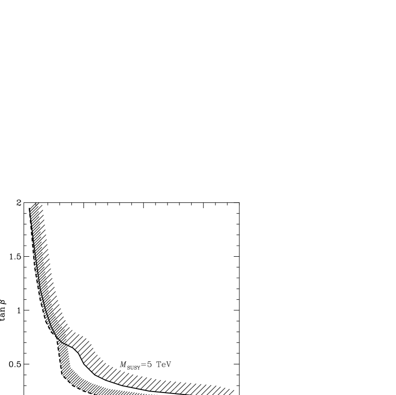
FIG. 1.: Region of parameter space $(M_{A},\tan\beta)$ where membrane solutions exist, for two different values of the supersymmetry-breaking mass $M_{\rm SUSY}$. Solutions exist below and to the left of the curves.

Solutions were sought for parameters in the ranges $0\leq\mu_{\!A}\equiv M_{A}/M_{Z}\leq 10$, $0.1<\tan\beta\leq 10$, and $0\leq t\equiv\ln(M_{\rm SUSY}^{\,2}/M_{t}^{\,2})\leq 10$. In agreement with the qualitative discussion of the previous section, we found no solutions for $t=0$ (tree level). For realistic values of $t$, corresponding to values of $M_{\rm SUSY}$ between $500$ GeV and $5$ TeV, solutions were found for $M_{A}\lower 3.01385pt\hbox{$\;\stackrel{{\scriptstyle\textstyle<}}{{\sim}}\;$}50$ GeV and for $\tan\beta\lower 3.01385pt\hbox{$\;\stackrel{{\scriptstyle\textstyle<}}{{\sim}}\;$}0.5$. The region of parameter space ($M_{A}$, $\tan\beta$) where solutions exist is shown in Fig. 1. Fig. 2 depicts a typical solution.

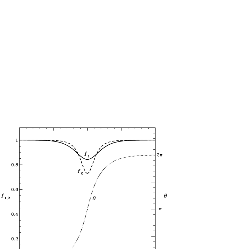
FIG. 2.: The membrane solution for $M_{A}=50$ GeV, $\tan\beta=0.5$ and $M_{\rm SUSY}=5$ TeV.

We used $M_{t}=175$ GeV, $v=246.2$ GeV, $M_{Z}=91.2$ GeV, $M_{W}=80.2$ GeV, and $g_{\rm s}^{2}/4\pi\equiv\alpha_{\rm s}=\alpha_{\rm s}(M_{t})=0.107$.

The solutions were unchanged as the number of grid points was doubled, and it was verified that they obey integral sum rules akin to the virial theorem. An independent run with $w$ fixed at $1$, taking as initial guesses the true solutions for adjacent values of $(\mu_{\!A},\tan\beta,t)$ rather than the sine-Gordon kink, gave the same region of existence of solutions. This region is also quite insensitive to changes in the value of the top-quark mass in the range $160$ GeV$\leq M_{t}\leq 190$ GeV.

V. CONCLUSIONS AND OUTLOOK

In this paper we have presented the results of a detailed investigation of non-topological and CP-violating static wall solutions in the framework of the Minimal Supersymmetric Standard Model. We have shown that membranes, characterized by a non-trivial winding of the relative $U(1)$ phase of the two Higgs fields in the direction orthogonal to the wall, do not exist when the Higgs potential is computed at tree level, but appear when quantum loop corrections to the Higgs potential are included.

Our results demonstrate that CP-violating membranes exist only for small values of the mass of the CP-odd Higgs boson. This does not come as a surprise. Indeed, it was shown on general grounds by Georgi and Pais [13] that gauge theories with perturbative spontaneous symmetry breaking may exhibit CP violation solely by the structure of quantum corrections to the tree-level potential. This may occur if and only if there exist light pseudoscalars at the one-loop level. Even though the Georgi-Pais theorem was proved only for spatially uniform CP-violating ground states, we conjecture that a similar conclusion may be attained for CP-violating solitons whose existence is due to quantum effects alone. In our case, the light pseudoscalar should be identified with the CP-odd Higgs boson.

We have presented our analysis in terms of the model parameters $\tan\beta$ and $M_{A}$; see Fig. 1. Let us now compare our results to the present experimental and theoretical bounds in the $(\tan\beta,M_{A})$ plane.

The value of $\tan\beta$ may be theoretically bounded from below by invoking some ideas from grand unified scenarios. Indeed, if one assumes the perturbative validity of the MSSM up to a scale of $\sim 10^{16}$ GeV (the so-called “desert” hypothesis), the low-energy value of the top Yukawa coupling $h_{t}$ no longer depends upon its ‘initial’ value at high scale. This is known as the quasi-infrared fixed-point solution and gives a theoretical prediction of the physical top-quark mass $M_{t}$ that, when combined with the experimental bound $M_{t}=(175\pm 6)$ GeV, leads to the bound $\tan\beta>1.4$ . The most recent experimental bound on $M_{A}$ has been given by the ALEPH Collaboration from the LEP run at 172 GeV [14]. Combining results from the channel productions $e^{+}e^{-}\rightarrow hA,hZ$ exclude a CP-odd Higgs boson lighter than about 62.5 GeV for $\tan\beta>1$. Comparing these bounds with the existence curves in Fig. 1, we may conclude that CP-violating membranes do not exist in the allowed region of parameter space $(M_{A},\tan\beta)$.

Despite the fact that the existence of these objects is experimentally ruled out today, we argue here that they may have existed and played a significant role during the electroweak phase transition.

The basic parameter which controls the existence of membranes is the squared mass $m_{3}^{\,2}$ which multiplies the operator $H_{1}H_{2}$ in the Higgs potential (3). It is connected to the physical CP-odd Higgs boson mass by the relation $m_{3}^{\,2}=M_{A}^{\,2}\sin 2\beta/2$. From our results we may conclude that CP-violating membranes exist (for $\tan\beta>1$) only if $m_{3}^{\,2}$ is very small, in contradiction with experimental bounds. However, plasma corrections coming from the thermal bath that constitutes the early Universe at temperature $T$ may drastically alter this conclusion. As a matter of fact, the zero-temperature parameter $m_{3}^{\,2}$ receives a large temperature-dependent correction $\Delta m_{3}^{\,2}(T)$ from the interactions of the Higgs fields with stops, charginos and neutralinos, which populate the plasma for temperatures larger than about 100 GeV [2]. As a consequence, it is the quantity $\overline{m}_{3}^{\,2}(T)=m_{3}^{\,2}+\Delta m_{3}^{\,2}(T)$ that really controls the existence of membranes in the thermal bath. Since $\Delta m_{3}^{\,2}(T)$ may be sizeble and negative [2], $\overline{m}_{3}^{\,2}(T)$ may be small and membranes may exist during the electroweak phase transition for zero-temperature values of $M_{A}$ that are in agreement with present experimental bounds [15].

At temperatures above the critical phase-transition temperature, the thermal fluctuations may spontaneously and abundantly produce membrane-like configurations. A naive estimate of the number density of membranes of size $R$ produced at temperature $T$ due to thermal fluctuations is $n(R,T)\sim T^{3}{\rm e}^{-F/T}$, where $F$ is the free energy of the membrane of size $R$. An educated guess is $F\sim\eta R^{2}$ where $\eta$ is the energy per unit area. The membranes have $\eta\sim 2M_{A}(T)v^{2}(T)$, where $M_{A}^{\,2}(T)=\overline{m}_{3}^{\,2}(T)\sin 2\beta/2$, and a typical size $R\sim M_{A}^{-1}(T)$ so that the associated free energy is given by $F\sim 2v^{2}(T)/M_{A}(T)$. The thermal nucleation rate $\Gamma$ at which they are formed is of the order of $T{\rm e}^{-F/T}$ and is much higher than the expansion rate of the Universe $H\sim T^{2}/M_{P\ell}$ $(M_{P\ell}=1.2\times 10^{19}$ GeV being the Planck mass) as long as $F/T<{\rm ln}(M_{P\ell}/T)$. To get a feel for the numbers: At $T\sim$ 100 GeV, $F/T$ should be smaller than 40 or so.

Membranes are expected to be produced in great abundance by thermal fluctuations. They decay just as fast, however, since their lifetime $\tau$ is determined by interactions with the surrounding plasma: $\tau\sim T^{-1}$.

At the electroweak phase transition, taking place at temperatures of the order of 100 GeV, the Standard Model gauge group $SU(2)_{\rm L}\otimes U(1)_{Y}$ breaks and the scalar fields acquire vacuum expectation values $\langle\phi_{1,2}(T)\rangle$. The transition may occur via nucleation of critical bubbles of radius $R_{c}$ (first-order phase transition) or by an anomalous growth of initial thermal fluctuations in the unstable modes (second-order phase transition). Membranes may still be thermally nucleated during this epoch, and their presence can affect the fate of the baryon asymmetry produced in the transition itself if it is of the first order [16]. In any scenario where the baryon asymmetry is generated during a first-order electroweak phase transition, the asymmetry is produced in the vicinity of critical bubble walls, and a strong constraint on the ratio between the vacuum expectation value of the Higgs field inside the bubble and the temperature must be imposed, $\langle\phi(T)\rangle/T>1$, where in our case $\phi(T)=\sqrt{\phi_{1}^{\,2}(T)+\phi_{2}^{\,2}(T)}$ [16]. This bound is necessary for the just created baryon asymmetry to survive the anomalous baryon-violating interactions inside the critical bubble, and may be translated into a severe upper bound on the physical mass $M_{h}$ of the scalar Higgs particle. Combining this bound with the LEP constraint rules out the possibility of electroweak baryogenesis in the Standard Model of electroweak interactions, but leaves room for electroweak baryogenesis in the Minimal Supersymmetric extension of the Standard Model [6,17].

Since the rate of anomalous baryon-number-violating processes scales like ${\rm exp}(-\langle\phi\rangle/T)$, it is clear that even a small change in the vacuum expectation value of the Higgs scalar field from its equilibrium value may be crucial for electroweak baryogenesis considerations. Because $R_{c}\gg M_{A}^{-1}(T)$, membranes may be thermally produced in large numbers inside the critical bubbles and eventually decay. Since the vacuum expectation value $\langle\phi(T)\rangle$ is reduced inside the membranes with respect to the value in the exterior of the membranes (see Fig. 2), baryon-number-violating processes may be activated in the membranes, causing a reduction of any preexisting baryon asymmetry. The spontaneous violation of CP inside the membranes may also play a significant role in this respect. These and other considerations are now under investigation [15].