Abstract

We evaluate the relic density of the lightest neutralino, the lightest supersymmetric particle, in the Minimal Supersymmetric extension of the Standard Model (MSSM). For the first time, we include all coannihilation processes between neutralinos and charginos for any neutralino mass and composition. We use the most sophisticated routines for integrating the cross sections and the Boltzmann equation. We properly treat (sub)threshold and resonant annihilations. We also include one-loop corrections to neutralino masses. We find that coannihilation processes are important not only for light higgsino-like neutralinos, as pointed out before, but also for heavy higgsinos and for mixed and gaugino-like neutralinos. Indeed, coannihilations should be included whenever $|\mu|\mathrel{\hbox to0.0pt{\lower 4.0pt\hbox{\hskip 1.0pt$\sim$}\hss}\raise 1.0pt\hbox{$<$}}2|M_{1}|$, independently of the neutralino composition. When $|\mu|\sim|M_{1}|$, coannihilations can increase or decrease the relic density in and out of the cosmologically interesting region. We find that there is still a window of light higgsino-like neutralinos that are viable dark matter candidates and that coannihilations shift the cosmological upper bound on the neutralino mass from 3 to 7 TeV.

1 Introduction

In the near future, it may become possible to constrain supersymmetry from high precision measurements of the cosmological parameters [1, 2], among which the dark matter density. It is therefore of great importance to calculate the relic density of the lightest neutralino as accurately as possible.

The lightest neutralino is one of the most promising candidates for the dark matter in the Universe. It is believed to be the lightest stable supersymmetric particle in the Minimal Supersymmetric extension of the Standard Model (MSSM). It is a linear combination of the superpartners of the neutral gauge and Higgs bosons.

The relic density of neutralinos in the MSSM has been calculated by several authors during the years [3, 4, 5, 6, 7, 8, 9] with various degrees of precision. A complete and precise calculation including relativistic Boltzmann averaging, subthreshold and resonant annihilations, and coannihilation processes is the purpose of this paper.

As pointed out by Griest and Seckel [5] one has to include coannihilations between the lightest neutralino and other supersymmetric particles heavier than the neutralino if they are close in mass. They considered coannihilations between the lightest neutralino and the squarks, which occur only accidentally when the squarks are only slightly heavier than the lightest neutralino. In contrast, Mizuta and Yamaguchi [7] pointed out an unavoidable mass degeneracy that greatly affects the neutralino relic density: the degeneracy between the lightest and next-to-lightest neutralinos and the lightest chargino when the neutralino is higgsino-like. They considered coannihilations between the lightest neutralino and the lightest chargino, but only for neutralinos lighter then the $W$ boson and only with an approximate relic density calculation. Moreover, they did not consider Higgs bosons in the final states.

Drees and Nojiri [8] included coannihilations into their relic density calculation, but only between the lightest and next-to-lightest neutralinos. These coannihilations are not as important as those studied by Mizuta and Yamaguchi. Recently, Drees et al. [9] re-investigated the relic density of light higgsino-like neutralinos. They included coannihilations between the lightest and next-to-lightest neutralinos as well as those between the lightest neutralino and the lightest chargino. They do however only consider $f\bar{f}$, $f\bar{f^{\prime}}$ and $\gamma W^{+}$ final states through $Z$ and $W$ exchange respectively, and do not consider $t$- and $u$-channel annihilation or Higgs bosons in the final states.

In this paper we perform a full calculation of the neutralino relic density for any neutralino mass and composition, including for the first time all coannihilations between neutralinos and charginos. We properly compute the thermal average, particularly in presence of thresholds and resonances in the annihilation cross sections. We include all two-body final states of neutralino-neutralino, neutralino-chargino and chargino-chargino annihilations. We leave coannihilations with squarks [5] for future work, since they only occur accidentally when the squarks happen to be close in mass to the lightest neutralino as opposed to the unavoidable mass degeneracy of the lightest two neutralinos and the lightest chargino for higgsino-like neutralinos.

In section 2, we define the MSSM model we use and in section 3 we describe how we generalize the Gondolo and Gelmini [10] formulas to solve the Boltzmann equation and perform the thermal averages when coannihilations are included. This is done in a very convenient way by introducing an effective invariant annihilation rate $W_{\rm eff}$. In section 4 we describe how we calculate all annihilation cross sections, and in section 5 we outline the numerical methods we use. We then discuss our survey of supersymmetric models in section 6, together with the experimental constraints we apply. We finally present our results on the neutralino relic density in section 7 and give some concluding remarks in section 8.

2 Definition of the Supersymmetric model

We work in the framework of the minimal supersymmetric extension of the standard model defined by, besides the particle content and gauge couplings required by supersymmetry, the superpotential (the notation used is similar to Ref. [11])

$$W=\epsilon_{ij}\left(-{\bf\hat{e}}_{R}^{*}{\bf Y}_{E}{\bf\hat{l}}^{i}_{L}{\hat{H}}^{j}_{1}-{\bf\hat{d}}_{R}^{*}{\bf Y}_{D}{\bf\hat{q}}^{i}_{L}{\hat{H}}^{j}_{1}+{\bf\hat{u}}_{R}^{*}{\bf Y}_{U}{\bf\hat{q}}^{i}_{L}{\hat{H}}^{j}_{2}-\mu{\hat{H}}^{i}_{1}{\hat{H}}^{j}_{2}\right)$$ (1)

and the soft supersymmetry-breaking potential

$$V_{{\rm soft}}=\epsilon_{ij}\left({\bf\tilde{e}}_{R}^{*}{\bf A}_{E}{\bf Y}_{E}{\bf\tilde{l}}^{i}_{L}H^{j}_{1}+{\bf\tilde{d}}_{R}^{*}{\bf A}_{D}{\bf Y}_{D}{\bf\tilde{q}}^{i}_{L}H^{j}_{1}-{\bf\tilde{u}}_{R}^{*}{\bf A}_{U}{\bf Y}_{U}{\bf\tilde{q}}^{i}_{L}H^{j}_{2}-B\mu H^{i}_{1}H^{j}_{2}+{\rm h.c.}\right)$$ (2)

$$+H^{i*}_{1}m_{1}^{2}H^{i}_{1}+H^{i*}_{2}m_{2}^{2}H^{i}_{2}$$

$$+{\bf\tilde{q}}_{L}^{i*}{\bf M}_{Q}^{2}{\bf\tilde{q}}^{i}_{L}+{\bf\tilde{l}}_{L}^{i*}{\bf M}_{L}^{2}{\bf\tilde{l}}^{i}_{L}+{\bf\tilde{u}}_{R}^{*}{\bf M}_{U}^{2}{\bf\tilde{u}}_{R}+{\bf\tilde{d}}_{R}^{*}{\bf M}_{D}^{2}{\bf\tilde{d}}_{R}+{\bf\tilde{e}}_{R}^{*}{\bf M}_{E}^{2}{\bf\tilde{e}}_{R}$$

$$+{1\over 2}M_{1}\tilde{B}\tilde{B}+{1\over 2}M_{2}\left(\tilde{W}^{3}\tilde{W}^{3}+2\tilde{W}^{+}\tilde{W}^{-}\right)+{1\over 2}M_{3}\tilde{g}\tilde{g}.$$

Here $i$ and $j$ are SU(2) indices ($\epsilon_{12}=+1$). The Yukawa couplings ${\bf Y}$, the soft trilinear couplings ${\bf A}$ and the soft sfermion masses ${\bf M}$ are $3\times 3$ matrices in generation space. $\bf\hat{e}$, $\bf\hat{l}$, $\bf\hat{u}$, $\bf\hat{d}$ and $\bf\hat{q}$ are the superfields of the leptons and sleptons and of the quarks and squarks. A tilde indicates their respective scalar components. The $L$ and $R$ subscripts on the sfermion fields refer to the chirality of their fermionic superpartners. $\tilde{B}$, $\tilde{W}^{3}$ and $\tilde{W}^{\pm}$ are the fermionic superpartners of the SU(2) gauge fields and $\tilde{g}$ is the gluino field. $\mu$ is the higgsino mass parameter, $M_{1}$, $M_{2}$ and $M_{3}$ are the gaugino mass parameters, $B$ is a soft bilinear coupling, and $m^{2}_{1,2}$ are Higgs mass parameters.

For $M_{1}$ and $M_{2}$ we make the usual GUT assumptions

$$M_{1} = \frac{5}{3}M_{2}\tan^{2}\theta_{W}\simeq 0.5M_{2}$$ (3)

$$M_{2} = \frac{\alpha_{\rm ew}}{\sin^{2}\theta_{W}\alpha_{s}}M_{3}\simeq 0.3M_{3}$$ (4)

where $\alpha_{\rm ew}$ is the fine-structure constant and $\alpha_{s}$ is the strong coupling constant.

Electroweak symmetry breaking is caused by both $H^{1}_{1}$ and $H^{2}_{2}$ acquiring vacuum expectation values,

$$\langle H^{1}_{1}\rangle=v_{1},\qquad\langle H^{2}_{2}\rangle=v_{2},$$ (5)

with $g^{2}(v_{1}^{2}+v_{2}^{2})=2m_{W}^{2}$, with the further assumption that vacuum expectation values of all other scalar fields (in particular, squarks and sleptons) vanish. This avoids color and/or charge breaking vacua. It is convenient to use expressions for the $Z$ boson mass, $m_{Z}^{2}={1\over 2}(g^{2}+g^{\prime 2})(v_{1}^{2}+v_{2}^{2})$ and the ratio of vacuum expectation values $\tan\beta=v_{2}/v_{1}$. $g$ and $g^{\prime}$ are the usual SU(2) and U(1) gauge coupling constants.

When diagonalizing the mass matrix for the scalar Higgs fields, besides a charged and a neutral would-be Goldstone bosons which become the longitudinal polarizations of the $W^{\pm}$ and $Z$ gauge bosons, one finds a neutral CP-odd Higgs boson $A$, two neutral CP-even Higgs bosons $H_{1,2}$ and a charged Higgs boson $H^{\pm}$. Choosing as independent parameter the mass $m_{A}$ of the CP-odd Higgs boson, the masses of the other Higgs bosons are given by

$${\cal M}^{2}_{H}=\left(\matrix{{m_{A}^{2}\cos^{2}\beta+m_{Z}^{2}\sin^{2}\beta+\Delta{\cal M}^{2}_{11}}&{-\sin\beta\cos\beta(m_{A}^{2}+m_{Z}^{2})+\Delta{\cal M}^{2}_{12}}\cr{-\sin\beta\cos\beta(m_{A}^{2}+m_{Z}^{2})+\Delta{\cal M}^{2}_{21}}&{m_{A}^{2}\sin^{2}\beta+m_{Z}^{2}\cos^{2}\beta+\Delta{\cal M}^{2}_{22}}}\right)$$ (6)

$$m^{2}_{H^{\pm}}=m_{A}^{2}+m_{W}^{2}+\Delta_{\pm}.$$ (7)

The quantities $\Delta{\cal M}^{2}_{ij}$ and $\Delta_{\pm}$ are the leading log two-loop radiative corrections coming from virtual (s)top and (s)bottom loops, calculated within the effective potential approach given in [12] (other references on radiative corrections are [13]). Diagonalization of ${\cal M}^{2}_{H}$ gives the two CP-even Higgs boson masses, $m_{H_{1,2}}$, and their mixing angle $\alpha$ ($-\pi/2<\alpha<0$).

The neutralinos $\tilde{\chi}^{0}_{i}$ are linear combinations of the superpartners of the neutral gauge bosons ${\tilde{B}}$, $\tilde{W}_{3}$ and of the neutral higgsinos ${\tilde{H}_{1}^{0}}$, ${\tilde{H}_{2}^{0}}$. In this basis, their mass matrix is given by

$${\cal M}_{\tilde{\chi}^{0}_{1,2,3,4}}=\left(\matrix{{M_{1}}&0&-{g^{\prime}v_{1}\over\sqrt{2}}&+{g^{\prime}v_{2}\over\sqrt{2}}\cr 0&{M_{2}}&+{gv_{1}\over\sqrt{2}}&-{gv_{2}\over\sqrt{2}}\cr-{g^{\prime}v_{1}\over\sqrt{2}}&+{gv_{1}\over\sqrt{2}}&\delta_{33}&-\mu\cr+{g^{\prime}v_{2}\over\sqrt{2}}&-{gv_{2}\over\sqrt{2}}&-\mu&\delta_{44}\cr}\right)$$ (8)

where $\delta_{33}$ and $\delta_{44}$ are the most important one-loop corrections. These can change the neutralino masses by a few GeV up or down and are only important when there is a severe mass degeneracy of the lightest neutralinos and/or charginos. The expressions for $\delta_{33}$ and $\delta_{44}$ are [9, 14]

$$\delta_{33} = -\frac{3}{16\pi^{2}}Y_{b}^{2}m_{b}\sin(2\theta_{\tilde{b}}){\rm Re}\left[B_{0}(Q,b,\tilde{b}_{1})-B_{0}(Q,b,\tilde{b}_{2})\right]$$ (9)

$$\delta_{44} = -\frac{3}{16\pi^{2}}Y_{t}^{2}m_{t}\sin(2\theta_{\tilde{t}}){\rm Re}\left[B_{0}(Q,t,\tilde{t}_{1})-B_{0}(Q,t,\tilde{t}_{2})\right]$$ (10)

where $m_{b}$ and $m_{t}$ are the masses of the $b$ and $t$ quarks, $Y_{b}=gm_{b}/\sqrt{2}m_{W}\cos\beta$ and $Y_{t}=gm_{t}/\sqrt{2}m_{W}\sin\beta$ are the Yukawa couplings of the $b$ and $t$ quark, $\theta_{\tilde{b}}$ and $\theta_{\tilde{t}}$ are the mixing angles of the squark mass eigenstates ($\tilde{q}_{1}=\tilde{q}_{L}\cos\theta_{\tilde{q}}+\tilde{q}_{R}\sin\theta_{\tilde{q}}$) and $B_{0}$ is the two-point function for which we use the convention in Ref. [9, 14]. Expressions for $B_{0}$ can be found in e.g. Ref. [15]. For the momentum scale $Q$ we use $|\mu|$ as suggested in Ref. [9]. Note that the loop corrections depend on the mixing angles of the squarks which in turn depend on the soft supersymmetry breaking parameters ${\bf A}_{U}$ and ${\bf A}_{D}$ in Eq. (2) (or the parameters $A_{b}$ and $A_{t}$ given below).

The neutralino mass matrix, Eq. (8), can be diagonalized analytically to give four neutral Majorana states,

$$\tilde{\chi}^{0}_{i}=N_{i1}\tilde{B}+N_{i2}\tilde{W}^{3}+N_{i3}\tilde{H}^{0}_{1}+N_{i4}\tilde{H}^{0}_{2},$$ (11)

the lightest of which, to be called $\chi$, is then the candidate for the particle making up the dark matter in the Universe. The gaugino fraction, $Z_{g}^{i}$ of neutralino $i$ is then defined as

$$Z_{g}^{i}=|N_{i1}|^{2}+|N_{i2}|^{2}$$ (12)

We will call the neutralino higgsino-like if $Z_{g}<0.01$, mixed if $0.01\leq Z_{g}\leq 0.99$ and gaugino-like if $Z_{g}>0.99$, where $Z_{g}\equiv Z_{g}^{1}$ is the gaugino fraction of the lightest neutralino. Note that the boundaries for what we call gaugino-like and higgsino-like are somewhat arbitrary and may differ from other authors.

The charginos are linear combinations of the charged gauge bosons ${\tilde{W}^{\pm}}$ and of the charged higgsinos ${\tilde{H}_{1}^{-}}$, ${\tilde{H}_{2}^{+}}$. Their mass terms are given by

$$\left(\matrix{{\tilde{W}^{-}}&{\tilde{H}_{1}^{-}}}\right)\>{\cal M}_{\tilde{\chi}^{\pm}}\>\left(\matrix{{\tilde{W}^{+}}\cr{\tilde{H}_{2}^{+}}}\right)+\mbox{\rm h.c.}$$ (13)

Their mass matrix,

$${\cal M}_{\tilde{\chi}^{\pm}}=\left(\matrix{{M_{2}}&{gv_{2}}\cr{gv_{1}}&\mu}\right),$$ (14)

is diagonalized by the following linear combinations

$$\tilde{\chi}^{-}_{i} = U_{i1}\tilde{W}^{-}+U_{i2}\tilde{H}_{1}^{-},$$ (15)

$$\tilde{\chi}^{+}_{i} = V_{i1}\tilde{W}^{+}+V_{i2}\tilde{H}_{2}^{+}.$$ (16)

We choose ${\rm det}(U)=1$ and $U^{*}{\cal M}_{\tilde{\chi}^{\pm}}V^{\dagger}={\rm diag}(m_{\tilde{\chi}^{\pm}_{1}},m_{\tilde{\chi}^{\pm}_{2}})$ with non-negative chargino masses $m_{\tilde{\chi}^{\pm}_{i}}\geq 0$. We do not include any one-loop corrections to the chargino masses since they are negligible compared to the corrections $\delta_{33}$ and $\delta_{44}$ introduced above for the neutralino masses [9].

When discussing the squark mass matrix including mixing, it is convenient to choose a basis where the squarks are rotated in the same way as the corresponding quarks in the standard model. We follow the conventions of the particle data group [16] and put the mixing in the left-handed $d$-quark fields, so that the definition of the Cabibbo-Kobayashi-Maskawa matrix is $\mbox{\bf K}=\mbox{\bf V}_{1}\mbox{\bf V}_{2}^{\dagger}$, where $\mbox{\bf V}_{1}$ ($\mbox{\bf V}_{2}$) rotates the interaction left-handed $u$-quark ($d$-quark) fields to mass eigenstates. For sleptons we choose an analogous basis, but due to the masslessness of neutrinos no analog of the CKM matrix appears.

We then obtain the general $6\times 6$ $\tilde{u}$- and $\tilde{d}$-squark mass matrices:

$${\cal M}_{\tilde{u}}^{2}=\left(\matrix{\mbox{\bf M}_{Q}^{2}+\mbox{\bf m}_{u}^{\dagger}\mbox{\bf m}_{u}+D_{LL}^{u}\mbox{\bf 1}&\mbox{\bf m}_{u}^{\dagger}({\bf A}_{U}^{\dagger}-\mu^{*}\cot\beta)\cr({\bf A}_{U}-\mu\cot\beta)\mbox{\bf m}_{u}&\mbox{\bf M}_{U}^{2}+\mbox{\bf m}_{u}\mbox{\bf m}_{u}^{\dagger}+D_{RR}^{u}\mbox{\bf 1}\cr}\right),$$ (17)

$${\cal M}_{\tilde{d}}^{2}=\left({\matrix{{\mbox{\bf K}^{\dagger}\mbox{\bf M}_{Q}^{2}\mbox{\bf K}+\mbox{\bf m}_{d}\mbox{\bf m}_{d}^{\dagger}+D_{LL}^{d}\mbox{\bf 1}}&{\mbox{\bf m}_{d}^{\dagger}({\bf A}_{D}^{\dagger}-\mu^{*}\tan\beta)}\cr{({\bf A}_{D}-\mu\tan\beta)\mbox{\bf m}_{d}}&{\mbox{\bf M}_{D}^{2}+\mbox{\bf m}_{d}^{\dagger}\mbox{\bf m}_{d}+D_{RR}^{d}\mbox{\bf 1}}\cr}}\right),$$ (18)

and the general sneutrino and charged slepton masses

$${\cal M}^{2}_{\tilde{\nu}}=\mbox{\bf M}_{L}^{2}+D^{\nu}_{LL}\mbox{\bf 1}$$ (19)

$${\cal M}^{2}_{\tilde{e}}=\left({\matrix{{\mbox{\bf M}_{L}^{2}+\mbox{\bf m}_{e}\mbox{\bf m}_{e}^{\dagger}+D_{LL}^{e}\mbox{\bf 1}}&{\mbox{\bf m}_{e}^{\dagger}({\bf A}_{E}^{\dagger}-\mu^{*}\tan\beta)}\cr{({\bf A}_{E}-\mu\tan\beta)\mbox{\bf m}_{e}}&{\mbox{\bf M}_{E}^{2}+\mbox{\bf m}_{e}^{\dagger}\mbox{\bf m}_{e}+D_{RR}^{e}\mbox{\bf 1}}\cr}}\right).$$ (20)

Here

$$D^{f}_{LL}=m_{Z}^{2}\cos 2\beta(T_{3f}-e_{f}\sin^{2}\theta_{W}),$$ (21)

$$D^{f}_{RR}=m_{Z}^{2}\cos 2\beta e_{f}\sin^{2}\theta_{W}$$ (22)

where $T_{3f}$ is the third component of the weak isospin and $e_{f}$ is the charge in units of the absolute value of the electron charge, $e$. In the chosen basis, we have $\mbox{\bf m}_{u}$ = $\mbox{\rm diag}\left(m_{\rm u},m_{\rm c},m_{\rm t}\right)$, $\mbox{\bf m}_{d}$ = $\mbox{\rm diag}\left(m_{\rm d},m_{\rm s},m_{\rm b}\right)$ and $\mbox{\bf m}_{e}$ = $\mbox{\rm diag}(m_{e},m_{\mu},m_{\tau})$.

The slepton and squark mass eigenstates $\tilde{f}_{k}$ ($\tilde{\nu}_{k}$ with $k=1,2,3$ and $\tilde{e}_{k}$, $\tilde{u}_{k}$ and $\tilde{d}_{k}$ with $k=1,\dots,6$) diagonalize the previous mass matrices and are related to the current sfermion eigenstates $\tilde{f}_{La}$ and $\tilde{f}_{Ra}$ ($a=1,2,3$) via

$$\tilde{f}_{La} = \sum_{k=1}^{6}\tilde{f}_{k}{\bf\Gamma}_{FL}^{*ka},$$ (23)

$$\tilde{f}_{Ra} = \sum_{k=1}^{6}\tilde{f}_{k}{\bf\Gamma}_{FR}^{*ka}.$$ (24)

The squark and charged slepton mixing matrices ${\bf\Gamma}_{UL,R}$, ${\bf\Gamma}_{DL,R}$ and ${\bf\Gamma}_{EL,R}$ have dimension $6\times 3$, while the sneutrino mixing matrix ${\bf\Gamma}_{\nu L}$ has dimension $3\times 3$.

For simplicity we make a simple Ansatz for the up-to-now arbitrary soft supersymmetry-breaking parameters:

$$\begin{array}[]{l}{\bf A}_{U}=\mbox{\rm diag}(0,0,A_{t})\\ {\bf A}_{D}=\mbox{\rm diag}(0,0,A_{b})\\ {\bf A}_{E}=0\\ \mbox{\bf M}_{Q}=\mbox{\bf M}_{U}=\mbox{\bf M}_{D}=\mbox{\bf M}_{E}=\mbox{\bf M}_{L}=m_{0}\mbox{\bf 1}.\end{array}$$ (25)

This allows the squark mass matrices to be diagonalized analytically. For example, for the top squark one has, in terms of the top squark mixing angle $\theta_{\tilde{t}}$,

$$\Gamma_{UL}^{\tilde{t}_{1}\tilde{t}}=\Gamma_{UR}^{\tilde{t}_{2}\tilde{t}}=\cos\theta_{\tilde{t}},\qquad\Gamma_{UL}^{\tilde{t}_{2}\tilde{t}}=-\Gamma_{UR}^{\tilde{t}_{1}\tilde{t}}=\sin\theta_{\tilde{t}}.$$ (26)

Notice that the Ansatz (25) implies the absence of tree-level flavor changing neutral currents in all sectors of the model.

3 The Boltzmann equation and thermal averaging

Griest and Seckel [5] have worked out the Boltzmann equation when coannihilations are included. We start by reviewing their expressions and then continue by rewriting them into a more convenient form that resembles the familiar case without coannihilations. This allows us to use similar expressions for calculating thermal averages and solving the Boltzmann equation whether coannihilations are included or not.

3.1 Review of the Boltzmann equation with coannihilations

Consider annihilation of $N$ supersymmetric particles $\chi_{i}$ ($i=1,\ldots,N$) with masses $m_{i}$ and internal degrees of freedom (statistical weights) $g_{i}$. Also assume that $m_{1}\leq m_{2}\leq\cdots\leq m_{N-1}\leq m_{N}$ and that $R$-parity is conserved. Note that for the mass of the lightest neutralino we will use the notation $m_{\chi}$ and $m_{1}$ interchangeably.

The evolution of the number density $n_{i}$ of particle $i$ is

$$\frac{dn_{i}}{dt} = -3Hn_{i}-\sum_{j=1}^{N}\langle\sigma_{ij}v_{ij}\rangle\left(n_{i}n_{j}-n_{i}^{\rm{eq}}n_{j}^{\rm{eq}}\right)$$ (27)

$$-\sum_{j\neq i}\big{[}\langle\sigma^{\prime}_{Xij}v_{ij}\rangle\left(n_{i}n_{X}-n_{i}^{\rm{eq}}n_{X}^{\rm{eq}}\right)-\langle\sigma^{\prime}_{Xji}v_{ij}\rangle\left(n_{j}n_{X}-n_{j}^{\rm{eq}}n_{X}^{\rm{eq}}\right)\big{]}$$

$$-\sum_{j\neq i}\big{[}\Gamma_{ij}\left(n_{i}-n_{i}^{\rm{eq}}\right)-\Gamma_{ji}\left(n_{j}-n_{j}^{\rm{eq}}\right)\big{]}.$$

The first term on the right-hand side is the dilution due to the expansion of the Universe. $H$ is the Hubble parameter. The second term describes $\chi_{i}\chi_{j}$ annihilations, whose total annihilation cross section is

$$\sigma_{ij} = \sum_{X}\sigma(\chi_{i}\chi_{j}\rightarrow X).$$ (28)

The third term describes $\chi_{i}\to\chi_{j}$ conversions by scattering off the cosmic thermal background,

$$\sigma^{\prime}_{Xij} = \sum_{Y}\sigma(\chi_{i}X\rightarrow\chi_{j}Y)$$ (29)

being the inclusive scattering cross section. The last term accounts for $\chi_{i}$ decays, with inclusive decay rates

$$\Gamma_{ij} = \sum_{X}\Gamma(\chi_{i}\rightarrow\chi_{j}X).$$ (30)

In the previous expressions, $X$ and $Y$ are (sets of) standard model particles involved in the interactions, $v_{ij}$ is the ‘relative velocity’ defined by

$$v_{ij}=\frac{\sqrt{(p_{i}\cdot p_{j})^{2}-m_{i}^{2}m_{j}^{2}}}{E_{i}E_{j}}$$ (31)

with $p_{i}$ and $E_{i}$ being the four-momentum and energy of particle $i$, and finally $n_{i}^{\rm{eq}}$ is the equilibrium number density of particle $\chi_{i}$,

$$n_{i}^{\rm{eq}}=\frac{g_{i}}{(2\pi)^{3}}\int d^{3}{\bf p}_{i}f_{i}$$ (32)

where ${\bf p}_{i}$ is the three-momentum of particle $i$, and $f_{i}$ is its equilibrium distribution function. In the Maxwell-Boltzmann approximation it is given by

$$f_{i}=e^{-E_{i}/T}.$$ (33)

The thermal average $\langle\sigma_{ij}v_{ij}\rangle$ is defined with equilibrium distributions and is given by

$$\langle\sigma_{ij}v_{ij}\rangle=\frac{\int d^{3}{\bf p}_{i}d^{3}{\bf p}_{j}f_{i}f_{j}\sigma_{ij}v_{ij}}{\int d^{3}{\bf p}_{i}d^{3}{\bf p}_{j}f_{i}f_{j}}$$ (34)

Normally, the decay rate of supersymmetric particles $\chi_{i}$ other than the lightest which is stable is much faster than the age of the universe. Since we have assumed $R$-parity conservation, all of these particles decay into the lightest one. So its final abundance is simply described by the sum of the density of all supersymmetric particles,

$$n=\sum_{i=1}^{N}n_{i}.$$ (35)

For $n$ we get the following evolution equation

$$\frac{dn}{dt}=-3Hn-\sum_{i,j=1}^{N}\langle\sigma_{ij}v_{ij}\rangle\left(n_{i}n_{j}-n_{i}^{\rm{eq}}n_{j}^{\rm{eq}}\right)$$ (36)

where the terms on the second and third lines in Eq. (27) cancel in the sum.

The scattering rate of supersymmetric particles off particles in the thermal background is much faster than their annihilation rate, because the scattering cross sections $\sigma^{\prime}_{Xij}$ are of the same order of magnitude as the annihilation cross sections $\sigma_{ij}$ but the background particle density $n_{X}$ is much larger than each of the supersymmetric particle densities $n_{i}$ when the former are relativistic and the latter are non-relativistic, and so suppressed by a Boltzmann factor. In this case, the $\chi_{i}$ distributions remain in thermal equilibrium, and in particular their ratios are equal to the equilibrium values,

$$\frac{n_{i}}{n}\simeq\frac{n_{i}^{\rm{eq}}}{n^{\rm{eq}}}.$$ (37)

We then get

$$\frac{dn}{dt}=-3Hn-\langle\sigma_{\rm{eff}}v\rangle\left(n^{2}-n_{\rm{eq}}^{2}\right)$$ (38)

where

$$\langle\sigma_{\rm{eff}}v\rangle=\sum_{ij}\langle\sigma_{ij}v_{ij}\rangle\frac{n_{i}^{\rm{eq}}}{n^{\rm{eq}}}\frac{n_{j}^{\rm{eq}}}{n^{\rm{eq}}}.$$ (39)

3.2 Thermal averaging

So far the reviewing. Now let’s continue by reformulating the thermal averages into more convenient expressions.

We rewrite Eq. (39) as

$$\langle\sigma_{\rm{eff}}v\rangle=\frac{\sum_{ij}\langle\sigma_{ij}v_{ij}\rangle n_{i}^{\rm{eq}}n_{j}^{\rm{eq}}}{n^{2}_{\rm{eq}}}=\frac{A}{n_{\rm{eq}}^{2}}\,.$$ (40)

For the denominator we obtain, using Boltzmann statistics for $f_{i}$,

$$n^{\rm eq}=\sum_{i}n^{\rm eq}_{i}=\sum_{i}\frac{g_{i}}{(2\pi)^{3}}\int d^{3}p_{i}e^{-E_{i}/T}=\frac{T}{2\pi^{2}}\sum_{i}g_{i}m_{i}^{2}K_{2}\left(\frac{m_{i}}{T}\right)$$ (41)

where $K_{2}$ is the modified Bessel function of the second kind of order 2.

The numerator is the total annihilation rate per unit volume at temperature $T$,

$$A=\sum_{ij}\langle\sigma_{ij}v_{ij}\rangle n_{i}^{\rm eq}n_{j}^{\rm eq}=\sum_{ij}\frac{g_{i}g_{j}}{(2\pi)^{6}}\int d^{3}{\bf p}_{i}d^{3}{\bf p}_{j}f_{i}f_{j}\sigma_{ij}v_{ij}$$ (42)

It is convenient to cast it in a covariant form,

$$A=\sum_{ij}\int W_{ij}\frac{g_{i}f_{i}d^{3}{\bf p}_{i}}{(2\pi)^{3}2E_{i}}\frac{g_{j}f_{j}d^{3}{\bf p}_{j}}{(2\pi)^{3}2E_{j}}.$$ (43)

$W_{ij}$ is the (unpolarized) annihilation rate per unit volume corresponding to the covariant normalization of $2E$ colliding particles per unit volume. $W_{ij}$ is a dimensionless Lorentz invariant, related to the (unpolarized) cross section through

$$W_{ij}=4p_{ij}\sqrt{s}\sigma_{ij}=4\sigma_{ij}\sqrt{(p_{i}\cdot p_{j})^{2}-m_{i}^{2}m_{j}^{2}}=4E_{i}E_{j}\sigma_{ij}v_{ij}.$$ (44)

Here

$$p_{ij}=\frac{\left[s-(m_{i}+m_{j})^{2}\right]^{1/2}\left[s-(m_{i}-m_{j})^{2}\right]^{1/2}}{2\sqrt{s}}$$ (45)

is the momentum of particle $\chi_{i}$ (or $\chi_{j}$) in the center-of-mass frame of the pair $\chi_{i}\chi_{j}$.

Averaging over initial and summing over final internal states, the contribution to $W_{ij}$ of a general $n$-body final state is

$$W^{n\rm{-body}}_{ij}=\frac{1}{g_{i}g_{j}S_{f}}\sum_{\rm{internal~{}d.o.f.}}\int\left|{\cal M}\right|^{2}(2\pi)^{4}\delta^{4}(p_{i}+p_{j}-{\textstyle\sum_{f}}p_{f})\prod_{f}\frac{d^{3}{\bf p}_{f}}{(2\pi)^{3}2E_{f}},$$ (46)

where $S_{f}$ is a symmetry factor accounting for identical final state particles (if there are $K$ sets of $N_{k}$ identical particles, $k=1,\dots,K$, then $S_{f}=\prod_{k=1}^{K}N_{k}!$). In particular, the contribution of a two-body final state can be written as

$$W^{\rm{2-body}}_{ij\to kl}=\frac{p_{kl}}{16\pi^{2}g_{i}g_{j}S_{kl}\sqrt{s}}\sum_{\rm{internal~{}d.o.f.}}\int\left|{\cal M}(ij\to kl)\right|^{2}d\Omega,$$ (47)

where $p_{kl}$ is the final center-of-mass momentum, $S_{kl}$ is a symmetry factor equal to 2 for identical final particles and to 1 otherwise, and the integration is over the outgoing directions of one of the final particles. As usual, an average over initial internal degrees of freedom is performed.

We now reduce the integral in the covariant expression for $A$, Eq. (43), from 6 dimensions to 1. Using Boltzmann statistics for $f_{i}$ (a good approximation for $T\mathrel{\hbox to0.0pt{\lower 4.0pt\hbox{\hskip 1.0pt$\sim$}\hss}\raise 1.0pt\hbox{$<$}}m$)

$$A=\sum_{ij}\int g_{i}g_{j}W_{ij}e^{-E_{i}/T}e^{-E_{j}/T}\frac{d^{3}{\bf p}_{i}}{(2\pi)^{3}2E_{i}}\frac{d^{3}{\bf p}_{j}}{(2\pi)^{3}2E_{j}},$$ (48)

where ${\bf p}_{i}$ and ${\bf p}_{j}$ are the three-momenta and $E_{i}$ and $E_{j}$ are the energies of the colliding particles. Following the procedure in Ref. [10] we then rewrite the momentum volume element as

$$d^{3}{\bf p}_{i}d^{3}{\bf p}_{j}=4\pi|{\bf p}_{i}|E_{i}dE_{i}\,4\pi|{\bf p}_{j}|E_{j}dE_{j}\,\frac{1}{2}d\cos\theta$$ (49)

where $\theta$ is the angle between ${\bf p}_{i}$ and ${\bf p}_{j}$. Then we change integration variables from $E_{i}$, $E_{j}$, $\theta$ to $E_{+}$, $E_{-}$ and $s$, given by

$$\left\{\begin{array}[]{lcl}E_{+}&=&E_{i}+E_{j}\\ E_{-}&=&E_{i}-E_{j}\\ s&=&m_{i}^{2}+m_{j}^{2}+2E_{i}E_{j}-2|{\bf p}_{i}||{\bf p}_{j}|\cos\theta,\end{array}\right.$$ (50)

whence the volume element becomes

$$\frac{d^{3}{\bf p}_{i}}{(2\pi)^{3}2E_{i}}\frac{d^{3}{\bf p}_{j}}{(2\pi)^{3}2E_{j}}=\frac{1}{(2\pi)^{4}}\frac{dE_{+}dE_{-}ds}{8},$$ (51)

and the integration region $\{E_{i}\geq m_{i},E_{j}\geq m_{j},|\cos\theta|\leq 1\}$ transforms into

$$s\geq(m_{i}+m_{j})^{2},$$ (52)

$$E_{+}\geq\sqrt{s},$$ (53)

$$\left|E_{-}-E_{+}\frac{m_{j}^{2}-m_{i}^{2}}{s}\right|\leq 2p_{ij}\sqrt{\frac{E_{+}^{2}-s}{s}}.$$ (54)

Notice now that the product of the equilibrium distribution functions depends only on $E_{+}$ and not $E_{-}$ due to the Maxwell-Boltzmann approximation, and that the invariant rate $W_{ij}$ depends only on $s$ due to the neglect of final state statistical factors. Hence we can immediately integrate over $E_{-}$,

$$\int dE_{-}=4p_{ij}\sqrt{\frac{E_{+}^{2}-s}{s}}.$$ (55)

The volume element is now

$$\frac{d^{3}{\bf p}_{i}}{(2\pi)^{3}2E_{i}}\frac{d^{3}{\bf p}_{j}}{(2\pi)^{3}2E_{j}}=\frac{1}{(2\pi)^{4}}\frac{p_{ij}}{2}\sqrt{\frac{E_{+}^{2}-s}{s}}dE_{+}ds$$ (56)

We now perform the $E_{+}$ integration. We obtain

$$A=\frac{T}{32\pi^{4}}\sum_{ij}\int_{(m_{i}+m_{j})^{2}}^{\infty}dsg_{i}g_{j}p_{ij}W_{ij}K_{1}\left(\frac{\sqrt{s}}{T}\right)$$ (57)

where $K_{1}$ is the modified Bessel function of the second kind of order 1.

We can take the sum inside the integral and define an effective annihilation rate $W_{\rm eff}$ through

$$\sum_{ij}g_{i}g_{j}p_{ij}W_{ij}=g_{1}^{2}p_{\rm{eff}}W_{\rm{eff}}$$ (58)

with

$$p_{\rm{eff}}=p_{11}=\frac{1}{2}\sqrt{s-4m_{1}^{2}}.$$ (59)

In other words

$$W_{\rm{eff}}=\sum_{ij}\frac{p_{ij}}{p_{11}}\frac{g_{i}g_{j}}{g_{1}^{2}}W_{ij}=\sum_{ij}\sqrt{\frac{[s-(m_{i}-m_{j})^{2}][s-(m_{i}+m_{j})^{2}]}{s(s-4m_{1}^{2})}}\frac{g_{i}g_{j}}{g_{1}^{2}}W_{ij}.$$ (60)

Because $W_{ij}(s)=0$ for $s\leq(m_{i}+m_{j})^{2}$, the radicand is never negative.

In terms of cross sections, this is equivalent to the definition

$$\sigma_{\rm eff}=\sum_{ij}\frac{p^{2}_{ij}}{p^{2}_{11}}\frac{g_{i}g_{j}}{g_{1}^{2}}\sigma_{ij}.$$ (61)

Eq. (57) then reads

$$A=\frac{g_{1}^{2}T}{32\pi^{4}}\int_{4m_{1}^{2}}^{\infty}dsp_{\rm eff}W_{\rm eff}K_{1}\left(\frac{\sqrt{s}}{T}\right)$$ (62)

This can be written in a form more suitable for numerical integration by using $p_{\rm{eff}}$ instead of $s$ as integration variable. From Eq. (59), we have $ds=8p_{\rm{eff}}dp_{\rm{eff}}$, and

$$A=\frac{g_{1}^{2}T}{4\pi^{4}}\int_{0}^{\infty}dp_{\rm eff}p^{2}_{\rm eff}W_{\rm eff}K_{1}\left(\frac{\sqrt{s}}{T}\right)$$ (63)

with

$$s=4p_{\rm{eff}}^{2}+4m_{1}^{2}$$ (64)

So we have succeeded in rewriting $A$ as a 1-dimensional integral.

From Eqs. (63) and (41), the thermal average of the effective cross section results

$$\langle\sigma_{\rm{eff}}v\rangle=\frac{\int_{0}^{\infty}dp_{\rm{eff}}p_{\rm{eff}}^{2}W_{\rm{eff}}K_{1}\left(\frac{\sqrt{s}}{T}\right)}{m_{1}^{4}T\left[\sum_{i}\frac{g_{i}}{g_{1}}\frac{m_{i}^{2}}{m_{1}^{2}}K_{2}\left(\frac{m_{i}}{T}\right)\right]^{2}}.$$ (65)

This expression is very similar to the case without coannihilations, the differences being the denominator and the replacement of the annihilation rate with the effective annihilation rate. In the absence of coannihilations, this expression correctly reduces to the formula in Gondolo and Gelmini [10].

The definition of an effective annihilation rate independent of temperature is a remarkable calculational advantage. As in the case without coannihilations, the effective annihilation rate can in fact be tabulated in advance, before taking the thermal average and solving the Boltzmann equation.

Figure 1: The effective invariant annihiliation rate $W_{\rm eff}$ as a function of $p_{\rm eff}$ for model 1 in Table 3. The final state threshold for annihilation into $W^{+}W^{-}$ and the coannihilation thresholds, as given by Eq. (60), are indicated. The $\chi_{2}^{0}\chi_{2}^{0}$ coannihilation threshold is too small to be seen.

In the effective annihilation rate, coannihilations appear as thresholds at $\sqrt{s}$ equal to the sum of the masses of the coannihilating particles. We show an example in Fig. 1 where it is clearly seen that the coannihilation thresholds appear in the effective invariant rate just as final state thresholds do. For the same example, Fig. 2 shows the differential annihilation rate per unit volume $dA/dp_{\rm eff}$, the integrand in Eq. (63), as a function of $p_{\rm eff}$. We have chosen a temperature $T=m_{\chi}/20$, a typical freeze-out temperature. The Boltzmann suppression contained in the exponential decay of $K_{1}$ at high $p_{\rm eff}$ is clearly visible. At higher temperatures the peak shifts to the right and at lower temperatures to the left. For the particular model shown in Figs. 1–2, the relic density results $\Omega_{\chi}h^{2}=0.030$ when coannihilations are included and $\Omega_{\chi}h^{2}=0.18$ when they are not. Coannihilations have lowered $\Omega_{\chi}h^{2}$ by a factor of 6.

Figure 2: Total differential annihilation rate per unit volume $dA/dp_{\rm eff}$ for the same model as in Fig. 1, evaluated at a temperature $T=m_{\chi}/20$, typical of freeze-out. Notice the Boltzmann suppression at high $p_{\rm eff}$.

We end this section with a comment on the internal degrees of freedom $g_{i}$. A neutralino is a Majorana fermion and has two internal degrees of freedom, $g_{\chi_{i}^{0}}=2$. A chargino can be treated either as two separate species $\chi_{i}^{+}$ and $\chi_{i}^{-}$, each with internal degrees of freedom $g_{\chi^{+}}=g_{\chi^{-}}=2$, or, more simply, as a single species $\chi_{i}^{\pm}$ with $g_{\chi_{i}^{\pm}}=4$ internal degrees of freedom. The effective annihilation rates involving charginos read

$$\left\{\begin{array}[]{lcl}W_{\chi_{i}^{0}\chi_{j}^{\pm}}&=&W_{\chi_{i}^{0}\chi_{j}^{+}}=W_{\chi_{i}^{0}\chi_{j}^{-}}\quad,\quad\forall\ i=1,\ldots,4,\ j=1,2\\[4.30554pt] W_{\chi_{i}^{\pm}\chi_{j}^{\pm}}&=&\frac{1}{2}\left[W_{\chi_{i}^{+}\chi_{j}^{+}}+W_{\chi_{i}^{+}\chi_{j}^{-}}\right]=\frac{1}{2}\left[W_{\chi_{i}^{-}\chi_{j}^{-}}+W_{\chi_{i}^{-}\chi_{j}^{+}}\right]\quad,\quad\forall\ i,j=1,2\end{array}\right.$$ (66)

3.3 Reformulation of the Boltzmann equation

We now follow Gondolo and Gelmini [10] to put Eq. (38) in a more convenient form by considering the ratio of the number density to the entropy density,

$$Y=\frac{n}{s}.$$ (67)

Consider

$$\frac{dY}{dt}=\frac{d}{dt}\left(\frac{n}{s}\right)=\frac{\dot{n}}{s}-\frac{n}{s^{2}}\dot{s}$$ (68)

where dot means time derivative. In absence of entropy production, $S=R^{3}s$ is constant ($R$ is the scale factor). Differentiating with respect to time we see that

$$\dot{s}=-3\frac{\dot{R}}{R}s=-3Hs$$ (69)

which yields

$$\dot{Y}=\frac{\dot{n}}{s}+3H\frac{n}{s}.$$ (70)

Hence we can rewrite Eq. (38) as

$$\dot{Y}=-s\langle\sigma_{\rm{eff}}v\rangle\left(Y^{2}-Y_{\rm{eq}}^{2}\right).$$ (71)

The right-hand side depends only on temperature, and it is therefore convenient to use temperature $T$ instead of time $t$ as independent variable. Defining $x=m_{1}/T$ we have

$$\frac{dY}{dx}=-\frac{m_{1}}{x^{2}}\frac{1}{3H}\frac{ds}{dT}\langle\sigma_{\rm{eff}}v\rangle\left(Y^{2}-Y_{\rm{eq}}^{2}\right).$$ (72)

where we have used

$$\frac{1}{\dot{T}}=\frac{1}{\dot{s}}\frac{ds}{dT}=-\frac{1}{3Hs}\frac{ds}{dT}$$ (73)

which follows from Eq. (69). With the Friedmann equation in a radiation dominated universe

$$H^{2}=\frac{8\pi G\rho}{3},$$ (74)

where $G$ is the gravitational constant, and the usual parameterization of the energy and entropy densities in terms of the effective degrees of freedom $g_{\rm{eff}}$ and $h_{\rm{eff}}$,

$$\rho=g_{\rm{eff}}(T)\frac{\pi^{2}}{30}T^{4},\quad s=h_{\rm{eff}}(T)\frac{2\pi^{2}}{45}T^{3},$$ (75)

we can cast Eq. (72) into the form [10]

$$\frac{dY}{dx}=-\sqrt{\frac{\pi}{45G}}\frac{g_{*}^{1/2}m_{1}}{x^{2}}\langle\sigma_{\rm{eff}}v\rangle\left(Y^{2}-Y_{\rm{eq}}^{2}\right)$$ (76)

where $Y_{\rm eq}$ can be written as

$$Y_{\rm{eq}}=\frac{n_{\rm{eq}}}{s}=\frac{45x^{2}}{4\pi^{4}h_{\rm{eff}}(T)}\sum_{i}g_{i}\left(\frac{m_{i}}{m_{1}}\right)^{2}K_{2}\left(x\frac{m_{i}}{m_{1}}\right),$$ (77)

using Eqs. (41), (67) and (75).

The parameter $g_{*}^{1/2}$ is defined as

$$g_{*}^{1/2}=\frac{h_{\rm{eff}}}{\sqrt{g_{\rm{eff}}}}\left(1+\frac{T}{3h_{\rm{eff}}}\frac{dh_{\rm{eff}}}{dT}\right)$$ (78)

For $g_{\rm eff}$, $h_{\rm eff}$ and $g_{*}^{1/2}$ we use the values in Ref. [10] with a QCD phase-transition temperature $T_{QCD}=150$ MeV. Our results are insensitive to the value of $T_{QCD}$, because due to a lower limit on the neutralino mass the neutralino freeze-out temperature is always much larger than $T_{QCD}$.

To obtain the relic density we integrate Eq. (76) from $x=0$ to $x_{0}=m_{\chi}/T_{0}$ where $T_{0}$ is the photon temperature of the Universe today. The relic density today in units of the critical density is then given by

$$\Omega_{\chi}=\rho_{\chi}^{0}/\rho_{\rm crit}=m_{\chi}s_{0}Y_{0}/\rho_{\rm crit}$$ (79)

where $\rho_{\rm crit}=3H^{2}/8\pi G$ is the critical density, $s_{0}$ is the entropy density today and $Y_{0}$ is the result of the integration of Eq. (76). With a background radiation temperature of $T_{0}=2.726$ K we finally obtain

$$\Omega_{\chi}h^{2}=2.755\times 10^{8}\frac{m_{\chi}}{\mbox{GeV}}Y_{0}.$$ (80)

4 Annihilation cross sections

Initial state	Final state	Feynman diagrams
	$H_{1}H_{1}$, $H_{1}H_{2}$, $H_{2}H_{2}$, $H_{3}H_{3}$	$t(\chi_{k}^{0})$, $u(\chi_{k}^{0})$, $s(H_{1,2})$
	$H_{1}H_{3}$, $H_{2}H_{3}$	$t(\chi_{k}^{0})$, $u(\chi_{k}^{0})$, $s(H_{3})$, $s(Z^{0})$
	$H^{-}H^{+}$	$t(\chi_{e}^{+})$, $u(\chi_{e}^{+})$, $s(H_{1,2})$, $s(Z^{0})$
	$Z^{0}H_{1}$, $Z^{0}H_{2}$	$t(\chi_{k}^{0})$, $u(\chi_{k}^{0})$, $s(H_{3})$, $s(Z^{0})$
$\chi_{i}^{0}\chi_{j}^{0}$	$Z^{0}H_{3}$	$t(\chi_{k}^{0})$, $u(\chi_{k}^{0})$, $s(H_{1,2})$
	$W^{-}H^{+}$, $W^{+}H^{-}$	$t(\chi_{e}^{+})$, $u(\chi_{e}^{+})$, $s(H_{1,2,3})$
	$Z^{0}Z^{0}$	$t(\chi_{k}^{0})$, $u(\chi_{k}^{0})$, $s(H_{1,2})$
	$W^{-}W^{+}$	$t(\chi_{e}^{+})$, $u(\chi_{e}^{+})$, $s(H_{1,2})$, $s(Z^{0})$
	$f\bar{f}$	$t(\tilde{f}_{L,R})$, $u(\tilde{f}_{L,R})$, $s(H_{1,2,3})$, $s(Z^{0})$
	$H^{+}H_{1}$, $H^{+}H_{2}$	$t(\chi_{k}^{0})$, $u(\chi_{e}^{+})$, $s(H^{+})$, $s(W^{+})$
	$H^{+}H_{3}$	$t(\chi_{k}^{0})$, $u(\chi_{e}^{+})$, $s(W^{+})$
	$W^{+}H_{1}$, $W^{+}H_{2}$	$t(\chi_{k}^{0})$, $u(\chi_{e}^{+})$, $s(H^{+})$, $s(W^{+})$
	$W^{+}H_{3}$	$t(\chi_{k}^{0})$, $u(\chi_{e}^{+})$, $s(H^{+})$
$\chi_{c}^{+}\chi_{i}^{0}$	$H^{+}Z^{0}$	$t(\chi_{k}^{0})$, $u(\chi_{e}^{+})$, $s(H^{+})$
	$\gamma H^{+}$	$t(\chi_{c}^{+})$, $s(H^{+})$
	$W^{+}Z^{0}$	$t(\chi_{k}^{0})$, $u(\chi_{e}^{+})$, $s(W^{+})$
	$\gamma W^{+}$	$t(\chi_{c}^{+})$, $s(W^{+})$
	$u\bar{d}$	$t(\tilde{d}_{L,R})$, $u(\tilde{u}_{L,R})$, $s(H^{+})$, $s(W^{+})$
	$\nu\bar{\ell}$	$t(\tilde{\ell}_{L,R})$, $u(\tilde{\nu}_{L})$, $s(H^{+})$, $s(W^{+})$
	$H_{1}H_{1}$, $H_{1}H_{2}$, $H_{2}H_{2}$, $H_{3}H_{3}$	$t(\chi_{e}^{+})$, $u(\chi_{e}^{+})$, $s(H_{1,2})$
	$H_{1}H_{3}$, $H_{2}H_{3}$	$t(\chi_{e}^{+})$, $u(\chi_{e}^{+})$, $s(H_{3})$, $s(Z^{0})$
	$H^{+}H^{-}$	$t(\chi_{k}^{0})$, $s(H_{1,2})$, $s(Z^{0},\gamma)$
	$Z^{0}H_{1}$, $Z^{0}H_{2}$	$t(\chi_{e}^{+})$, $u(\chi_{e}^{+})$, $s(H_{3})$, $s(Z^{0})$
	$Z^{0}H_{3}$	$t(\chi_{e}^{+})$, $u(\chi_{e}^{+})$, $s(H_{1,2})$
	$H^{+}W^{-}$, $W^{+}H^{-}$	$t(\chi_{e}^{+})$, $s(H_{1,2,3})$
$\chi_{c}^{+}\chi_{d}^{-}$	$Z^{0}Z^{0}$	$t(\chi_{e}^{+})$, $u(\chi_{e}^{+})$, $s(H_{1,2})$
	$W^{+}W^{-}$	$t(\chi_{k}^{0})$, $s(H_{1,2})$, $s(Z^{0},\gamma)$
	$\gamma\gamma$ (only for $c=d$)	$t(\chi_{c}^{+})$, $u(\chi_{c}^{+})$
	$Z^{0}\gamma$	$t(\chi_{d}^{+})$, $u(\chi_{c}^{+})$
	$u\bar{u}$	$t(\tilde{d}_{L,R})$, $s(H_{1,2,3})$, $s(Z^{0},\gamma)$
	$\nu\bar{\nu}$	$t(\tilde{\ell}_{L,R})$, $s(Z^{0})$
	$\bar{d}d$	$t(\tilde{u}_{L,R})$, $s(H_{1,2,3})$, $s(Z^{0},\gamma)$
	$\bar{\ell}\ell$	$t(\tilde{\nu}_{L})$, $s(H_{1,2,3})$, $s(Z^{0},\gamma)$
	$H^{+}H^{+}$	$t(\chi_{k}^{0})$, $u(\chi_{k}^{0})$
$\chi_{c}^{+}\chi_{d}^{+}$	$H^{+}W^{+}$	$t(\chi_{k}^{0})$, $u(\chi_{k}^{0})$
	$W^{+}W^{+}$	$t(\chi_{k}^{0})$, $u(\chi_{k}^{0})$

Table 1: All Feynman diagrams for which we calculate the annihilation cross section. $s(x)$, $t(x)$ and $u(x)$ denote a tree-level Feynman diagram in which particle $x$ is exchanged in the $s$-, $t$- and $u$-channel respectively. Indices $i,j,k$ run from 1 to 4, and indices $c,d,e$ from 1 to 2. $u$, $\tilde{u}$, $d$, $\tilde{d}$, $\nu$, $\tilde{\nu}$, $\ell$, $\tilde{\ell}$, $f$ and $\tilde{f}$ are generic notations for up-type quarks, up-type squarks, down-type quarks, down-type squarks, neutrinos, sneutrinos, leptons, sleptons, fermions and sfermions. A sum of diagrams over (s)fermion generation indices and over the neutralino and chargino indices $k$ and $e$ is understood (no sum over indices $i,j,c,d$).

We have calculated all two-body final state cross sections at tree level for neutralino-neutralino, neutralino-chargino and chargino-chargino annihilation. A complete list is given in Table 1.

Since we have so many different diagrams contributing, we have to use some method where the diagrams can be calculated efficiently. To achieve this, we classify diagrams according to their topology ($s$-, $t$- or $u$-channel) and to the spin of the particles involved. We then compute the helicity amplitudes for each type of diagram analytically with Reduce [17] using general expressions for the vertex couplings. Further details will be found in Ref. [18].

The strength of the helicity amplitude method is that the analytical calculation of a given type of diagram has to be performed only once and the sum of the contributing diagrams for each set of initial and final states can be done numerically afterwards.

5 Numerical methods

In this section we describe the numerical methods we use to evaluate the effective invariant rate and its thermal average, and to integrate the density evolution equation.

We obtain the effective invariant rate numerically as follows. We generate Fortran routines for the helicity amplitudes of all types of diagrams automatically with Reduce, as explained in the previous section. We sum the Feynman diagrams numerically for each annihilation channel $ij\to kl$. We then sum the squares of the helicity amplitudes so obtained, and sum the contributions of all annihilation channels. Explicitly, we compute

$${dW_{\rm eff}\over d\cos\theta}=\sum_{ijkl}{p_{ij}p_{kl}\over 32\pi p_{\rm eff}S_{kl}\sqrt{s}}\sum_{\rm helicities}\left|\sum_{\rm diagrams}{\cal M}(ij\to kl)\right|^{2}$$ (81)

where $\theta$ is the angle between particles $k$ and $i$. (We set $g_{1}=2$ as appropriate for a neutralino.)

We integrate over $\cos\theta$ numerically by means of adaptive gaussian integration. In rare cases, we find resonances in the $t$- or $u$-channels. For the process $ij\to kl$, this can occur when $m_{i}<m_{k}$ and $m_{j}>m_{l}$ or $m_{i}<m_{l}$ and $m_{j}>m_{k}$: at certain values of $\cos\theta$, the momentum transfer is time-like and matches the mass of the exchanged particle. We have regulated the divergence by assigning a small width of a few GeV to the neutralinos and charginos. Our results are not sensitive to the choice of this width.

The calculation of the effective invariant rate $W_{\rm eff}$ is the most time-consuming part. Fortunately, thanks to the remarkable feature of Eq. (65), $W_{\rm eff}(p_{\rm eff})$ does not depend on the temperature $T$, and it can be tabulated once for each model. We have to make sure that the maximum $p_{\rm eff}$ in the table is large enough to include all important resonances, thresholds and coannihilation thresholds. In the thermal average, the effective invariant rate is weighted by $K_{1}p_{\rm eff}^{2}$ (see Eq. (65)). The fast exponential decay of $K_{1}$ at high $p_{\rm eff}$ Boltzmann suppresses resonances and thresholds, as we have already seen in the example in Fig. 2. With a typical freeze-out temperature $T=m_{\chi}/20$, contributions to the thermal average from values of $p_{\rm eff}$ beyond $\sim 1.5m_{\chi}$ are negligible, even in the most extreme case we met in which the effective invariant rate at high $p_{\rm eff}$ was $10^{10}$ times higher than at $p_{\rm eff}=0$. For coannihilations, this value of $p_{\rm eff}$ corresponds to a mass of the coannihilating particle of $\sim 1.8m_{\chi}$. To be on the safe side all over parameter space, we include coannihilations whenever the mass of the coannihilating particle is less than $2.1m_{\chi}$, even if typically coannihilations are important only for masses less than $1.4m_{\chi}$. For extra safety, we tabulate $W_{\rm eff}$ from $p_{\rm eff}=0$ up to $p_{\rm eff}=20m_{\chi}$, more densely in the important low $p_{\rm eff}$ region than elsewhere. We further add several points around resonances and thresholds, both explicitly and in an adaptive manner.

To perform the thermal average in Eq. (65), we integrate over $p_{\rm eff}$ by means of adaptive gaussian integration, using a spline to interpolate in the $(p_{\rm eff},W_{\rm eff})$ table. To avoid numerical problems in the integration routine or in the spline routine, we split the integration interval at each sharp threshold. We also explicitly check for each MSSM model that the spline routine behaves well at thresholds and resonances.

We finally integrate the density evolution equation (76) numerically from $x=2$, where the density still tracks the equilibrium density, to $x_{0}=m_{\chi}/T_{0}$. We use an implicit trapezoidal method with adaptive stepsize. The method is implicit because of the stiffness of the evolution equation. The relic density at present is then evaluated with Eq. (80).

A more detailed description of the numerical methods will be found in a future publication [19].

6 Selection of models

Scan	normal	generous	light	high	high	light	heavy
			Higgs	mass 1	mass 2	higgsinos	gauginos
$\mu^{\rm min}$ [GeV]	$-5000$	$-10000$	$-5000$	1000	$-30000$	$-100$	1000
$\mu^{\rm max}$ [GeV]	5000	10000	5000	30000	$-1000$	100	30000
$M_{2}^{\rm min}$ [GeV]	$-5000$	$-10000$	$-5000$	1000	1000	$-1000$	1.9$\mu$/$-1.9\mu$
$M_{2}^{\rm max}$ [GeV]	5000	10000	5000	30000	30000	1000	2.1$\mu$/$-2.1\mu$
$\tan\beta^{\rm min}$	1.2	1.2	1.2	1.2	1.2	1.2	1.2
$\tan\beta^{\rm max}$	50	50	50	50	50	2.1	50
$m_{A}^{\rm min}$ [GeV]	0	0	0	0	0	0	0
$m_{A}^{\rm max}$ [GeV]	1000	3000	150	10000	10000	1000	10000
$m_{0}^{\rm min}$ [GeV]	100	100	100	1000	1000	100	1000
$m_{0}^{\rm max}$ [GeV]	3000	5000	3000	30000	30000	3000	30000
$A_{b}^{\rm min}$	$-3m_{0}$	$-3m_{0}$	$-3m_{0}$	$-3m_{0}$	$-3m_{0}$	$-3m_{0}$	$-3m_{0}$
$A_{b}^{\rm max}$	$3m_{0}$	$3m_{0}$	$3m_{0}$	$3m_{0}$	$3m_{0}$	$3m_{0}$	$3m_{0}$
$A_{t}^{\rm min}$	$-3m_{0}$	$-3m_{0}$	$-3m_{0}$	$-3m_{0}$	$-3m_{0}$	$-3m_{0}$	$-3m_{0}$
$A_{t}^{\rm max}$	$3m_{0}$	$3m_{0}$	$3m_{0}$	$3m_{0}$	$3m_{0}$	$3m_{0}$	$3m_{0}$
No. of models	4655	3938	3342	1000	999	177	250

Table 2: The ranges of parameter values in our scans of supersymmetric models. For $\mu$ and $M_{2}$ the scans are uniform in the logarithms of the parameters and for the rest they are uniform in the parameters themselves. The number of models refers to the number of generated models satisfying experimental constraints.

In Section 2 we made some simplifying assumptions to reduce the number of parameters in the MSSM to the seven parameters $\mu$, $M_{2}$, $\tan\beta$, $m_{A}$, $m_{0}$, $A_{b}$ and $A_{t}$. It is however a non-trivial task to scan even this reduced parameter space to a high degree of completeness. With the goal to explore a significant fraction of parameter space, we perform many different scans, some general and some specialized to interesting parts of parameter space. The ranges of parameter values in our scans are given in Table 2.

We perform a ‘normal’ scan where we let the seven free parameters above vary at random within wide ranges, a ‘generous’ scan with even more generous bounds on the parameters, a ‘light Higgs’ scan where we restrict to low pseudoscalar Higgs masses, and two ‘high mass’ scans where we explore heavy neutralinos. In addition we perform two other special scans: one to finely sample the cosmologically interesting light higgsino region, the other to study heavy mixed and gaugino-like neutralinos for which we found that coannihilations are important.

Remember, though, that the look of our figures might change if different scans were used. One should especially pay no attention to the density of points in different regions: it is just an artifact of our scanning.

We keep only models that satisfy the experimental constraints on squark, slepton, gluino, chargino, neutralino, and Higgs boson masses, on the $Z^{0}$ width and on the $b\rightarrow s\gamma$ branching ratio [16, 20, 21]. The last row in Table 2 gives the number of models which pass all experimental constraints. We include the most recent LEP2 constraints [20] of which the most important one is

$$m_{\chi^{+}}>85\mbox{ GeV}.$$ (82)

This bound effectively excludes most of the higgsinos lighter than the $W$ studied in Refs. [7, 9]. LEP2 also puts a new constraint on the lightest Higgs boson mass,

$$m_{H_{2}^{0}}>62.5\mbox{ GeV,}$$ (83)

valid for all $\alpha$ and $\beta$. This constraint could be made more stringent if allowed to depend on $\sin^{2}(\beta-\alpha)$, but we do not include this more refined version because in this study we are not very sensitive to this constraint.

7 Results

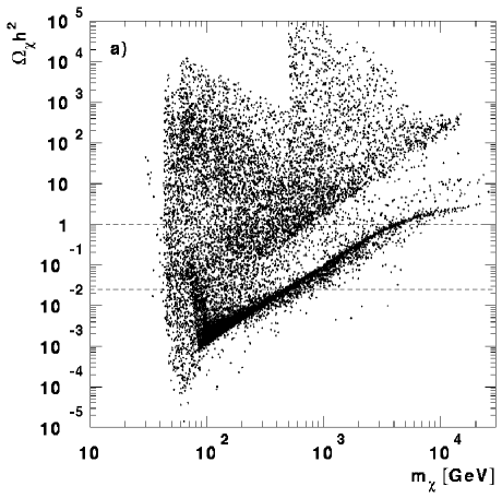
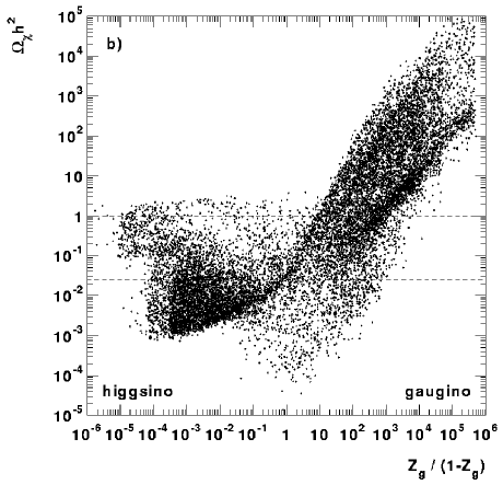
Figure 3: Neutralino relic density including neutralino and chargino coannihilations versus (a) neutralino mass $m_{\chi}$ and (b) neutralino composition $Z_{g}/(1-Z_{g})$. The horizontal lines bound the cosmologically interesting region $0.025<\Omega_{\chi}h^{2}<1$.

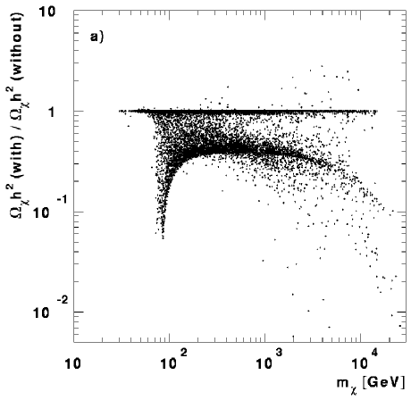
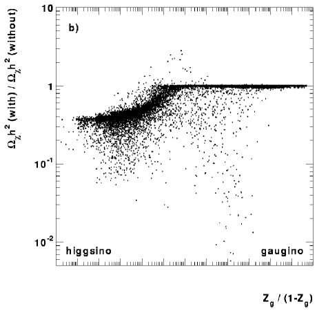
Figure 4: Ratio of the neutralino relic densities with and without neutralino and chargino coannihilations versus (a) neutralino mass $m_{\chi}$ and (b) neutralino composition $Z_{g}/(1-Z_{g})$.

We now present the results of our relic density calculations for all the models in Table 2. This is the first detailed evaluation of the neutralino relic density including neutralino and chargino coannihilations for general neutralino masses and compositions. So we focus on the effect of coannihilations.

Fundamentally, we are interested in how the inclusion of coannihilations modifies the cosmologically interesting region and the cosmological bounds on the neutralino mass. We define the cosmologically interesting region as $0.025<\Omega_{\chi}h^{2}<1$. In this range of $\Omega_{\chi}h^{2}$ the neutralino can constitute most of the dark matter in galaxies and the age of the Universe is long enough to be compatible with observations. The lower bound of 0.025 is somewhat arbitrary, and even if $\Omega_{\chi}h^{2}$ would be less than $0.025$ the neutralinos would still be relic particles, but only a minor fraction of the dark matter in the Universe.

We start with a short general discussion and then present more details in the following subsections.

Fig. 3 shows the neutralino relic density $\Omega_{\chi}h^{2}$ with coannihilations included versus the neutralino mass $m_{\chi}$ and the neutralino composition $Z_{g}/(1-Z_{g})$. The lower edge on neutralino masses comes essentially from the LEP bound on the chargino mass, Eq. (82). The few scattered points at the smallest masses have low $\tan\beta$. The bands and holes in the point distributions, and the lower edge in $Z_{g}/(1-Z_{g})$, are mere artifacts of our sampling in parameter space.

The neutralino is a good dark matter candidate in the region limited by the two horizontal lines (the cosmologically interesting region). There are clearly models with cosmologically interesting relic densities for a wide range of neutralino masses (up to 7 TeV) and compositions (up to $10^{-4}$ in higgsino fraction $Z_{h}=1-Z_{g}$). A plot of the cosmologically interesting region in the neutralino mass–composition plane is in subsection 7.5.

The effect of neutralino and chargino coannihilations on the value of the relic density is summarized in Fig. 4, where we plot the ratio of the neutralino relic densities with and without coannihilations versus the neutralino mass $m_{\chi}$ and the neutralino composition $Z_{g}/(1-Z_{g})$. In many models, coannihilations reduce the relic density by more than a factor of ten, and in some others they increase it by a small factor. Coannihilations increase the relic density if the effective annihilation cross section $\langle\sigma_{\rm eff}v\rangle<\langle\sigma_{11}v_{11}\rangle$. Recalling that $\langle\sigma_{\rm eff}v\rangle$ is the average of the coannihilation cross sections (see Eq. (40)), this occurs when most of the coannihilation cross sections are smaller than $\langle\sigma_{11}v_{11}\rangle$ and the mass differences are small.

Table 3 lists some representative models where coannihilations are important, one (or two) for each case described in the following subsections, plus one model where coannihilations are negligible. Example 1 contains a light higgsino-like neutralino, example 2 a heavy higgsino-like neutralino. Examples 3 and 4 have $|\mu|\sim|M_{1}|$, and example 5 has a very pure gaugino-like neutralino. Example 6 is a model with a gaugino-like neutralino for which coannihilations are not important.

	light	heavy	$|\mu|\sim|M_{1}|$		$|\mu|\gg|M_{1}|$	gaugino
	higgsino	higgsino			bino
Example No.	1	2	3	4	5	6
$\mu$ [GeV]	$77.7$	1024.3	358.7	414.7	$-7776.7$	$-1711.1$
$M_{2}$ [GeV]	$-441.4$	3894.1	$-691.1$	$-1154.6$	$133.5$	396.6
$\tan\beta$	1.31	40.0	2.00	7.30	37.0	22.8
$m_{A}$ [GeV]	656.8	737.2	577.7	828.9	2039.5	435.1
$m_{0}$ [GeV]	610.8	1348.3	1080.9	2237.9	4698.0	2771.6
$A_{b}/m_{0}$	$-1.77$	$-1.53$	$-1.03$	$-1.26$	$0.46$	1.97
$A_{t}/m_{0}$	2.75	$-2.01$	$-2.77$	$-0.80$	$0.11$	0.52
$m_{\chi_{1}^{0}}$ [GeV]	76.3	1020.8	340.2	407.8	67.2	199.5
$Z_{g}$	0.00160	0.00155	0.651	0.0262	0.999968	0.99933
$m_{\chi_{2}^{0}}$ [GeV]	96.3	1026.4	364.5	418.2	133.5	396.0
$m_{\chi_{1}^{+}}$ [GeV]	89.2	1023.7	362.2	414.1	133.5	396.0
$\Omega_{\chi}h^{2}$ (no coann.)	0.178	0.130	0.158	0.00522	$1.33\times 10^{4}$	0.418
$\Omega_{\chi}h^{2}$	0.0299	0.0388	0.0528	0.00905	$1.15\times 10^{4}$	0.418

Table 3: Some representative models for which coannihilations are important (examples 1–5) and one model (example 6) for which they are not. We give the seven model parameters, the masses of the lightest neutralinos and of the lightest chargino, the gaugino fraction of the lightest neutralino and the relic densities with and without coannihilations.

We have looked for a simple general criterion for when coannihilations should be included, one that goes beyond the trivial statement of an almost degeneracy in mass between the lightest neutralino and other supersymmetric particles. We have only found few rules of thumb, each with important exceptions. We give here the best two.

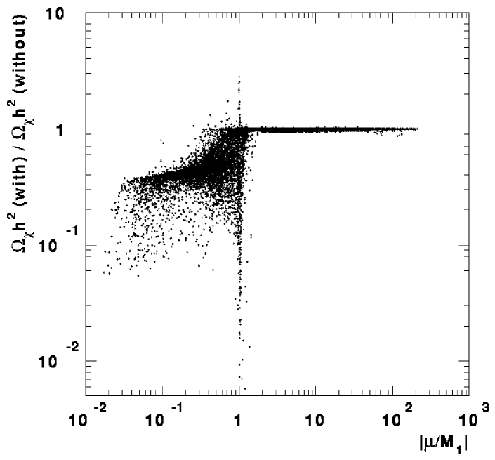
Figure 5: Ratio of the relic densities with and without coannihilations versus $|\mu/M_{1}|$. Coannihilations are important when $|\mu/M_{1}|\mathrel{\hbox to0.0pt{\lower 4.0pt\hbox{\hskip 1.0pt$\sim$}\hss}\raise 1.0pt\hbox{$<$}}2$.

The first rule of thumb is that when coannihilations are important, $|\mu/M_{1}|\mathrel{\hbox to0.0pt{\lower 4.0pt\hbox{\hskip 1.0pt$\sim$}\hss}\raise 1.0pt\hbox{$<$}}2$. But exceptions are found, as can be seen in Fig. 5, where we show the reduction in relic density due to the inclusion of coannihilations as a function of $|\mu/M_{1}|$. Notice that when $|\mu/M_{1}|\ll 1$, the neutralino is higgsino-like; when $|\mu/M_{1}|\gg 1$, the neutralino is gaugino-like; and when $|\mu/M_{1}|\sim 1$, the neutralino can be higgsino-like, gaugino-like or mixed.

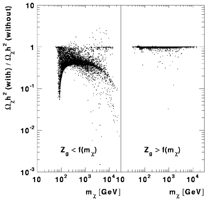
Figure 6: Ratio of the relic densities with and without coannihilations versus neutralino mass $m_{\chi}$. Coannihilations are generally not important when $Z_{g}>f(m_{\chi})$, where $f(m_{\chi})$ is the ’second rule of thumb’ given in the text.

The second rule of thumb is that coannihilations are important when $Z_{g}<0.23$ for $m_{\chi}<200$ GeV and when $Z_{g}/(1-Z_{g})<(m_{\chi}/300\mbox{ GeV})^{3}$ for $m_{\chi}>200$ GeV. There are exceptions to this rule, as can be seen in Fig. 6 where the ratio of relic densities with and without coannihilations is plotted versus the neutralino mass, the left panel for points satisfying the present criterion, the right panel for those not satisfying it.

In the following subsections, we present the cases where we found that coannihilations are important and explain why. We first discuss the already known case of light higgsino-like neutralinos, continue with heavier higgsino-like neutralinos, the case $|\mu|\sim|M_{1}|$ and finally very pure gaugino-like neutralinos. We then end this section by a discussion of the cosmologically interesting region.

7.1 Light higgsino-like neutralinos

We first discuss light higgsino-like neutralinos, $m_{\chi}<m_{W}$, $Z_{g}<0.01$, since coannihilation processes for these have been investigated earlier by other authors [7, 8, 9].

Mizuta and Yamaguchi [7] stressed the great importance of including coannihilations for higgsinos lighter than the $W$ boson. For these light higgsinos, neutralino-neutralino annihilation into fermions is strongly suppressed whereas chargino-neutralino and chargino-chargino annihilations into fermions are not. Since the masses of the lightest neutralino and the lightest chargino are of the same order, the relic density is greatly reduced when coannihilations are included. Mizuta and Yamaguchi claim that because of this reduction light higgsinos are cosmologically of no interest.

Drees and Nojiri [8] included coannihilations between the lightest and next-to-lightest neutralino, but overlooked those between the lightest neutralino and chargino, which are always more important. In spite of this, they concluded that the relic density of a higgsino-like neutralino will always be uninterestingly small unless $m_{\chi}>500$ GeV or so.

Drees at al. [9] then re-investigated the relic density of light higgsino-like neutralinos. They found that light higgsinos could have relic densities as high as 0.2, and so be cosmologically interesting, provided one-loop corrections to the neutralino masses are included.

We agree with these papers qualitatively, but we reach different conclusions. We show our results in Fig. 7, where we plot the relic density of higgsino-like neutralinos versus their mass with coannihilations included, as well as the ratio between the relic densities with and without coannihilations. The Mizuta and Yamaguchi reduction can be seen in Fig. 7b below 100 GeV, but due to the recent LEP2 bound on the chargino mass the effect is not as dramatic as it was for them. If for the sake of comparison we relax the LEP2 bound, the reduction continues down to $10^{-5}$ at lower higgsino masses and we confirm qualitatively the Mizuta and Yamaguchi conclusion — coannihilations are very important for light higgsinos — but we differ from them quantitatively since we find models in which light higgsinos have a cosmologically interesting relic density. For the specific light higgsino models in Drees et al. [9] we agree on the relic density to within 20–30%. We find however other light higgsino-like models with higher $\Omega_{\chi}h^{2}\sim 0.3$, even without including the loop corrections to the neutralino masses.

Figure 7: For higgsino-like neutralinos ($Z_{g}<0.01$) we show (a) the relic density with coannihilations included and (b) the ratio of the relic densities with and without coannihilations versus the neutralino mass. The horizontal lines in (a) limit the cosmologically interesting region $0.025<\Omega_{\chi}h^{2}<1$.

So there is a window of light higgsino models, $m_{\chi}\sim 75$ GeV, that are cosmologically interesting. All these models have $\tan\beta\mathrel{\hbox to0.0pt{\lower 4.0pt\hbox{\hskip 1.0pt$\sim$}\hss}\raise 1.0pt\hbox{$<$}}1.6$ and those with the highest relic densities have $\tan\beta\sim 1.2$. These models escape the LEP2 bound on the chargino mass, $m_{\chi^{+}}\sim 85$ GeV, because for $\tan\beta\mathrel{\hbox to0.0pt{\lower 4.0pt\hbox{\hskip 1.0pt$\sim$}\hss}\raise 1.0pt\hbox{$<$}}2$ the mass of the lightest neutralino can be lower than the mass of the lightest chargino by tens of GeV. By the same token, coannihilation processes are not so important and the relic density in these models remains cosmologically interesting. Most of these models will be probed in the near future when LEP2 runs at higher energies, but some have too large a chargino mass ($m_{\chi}^{+}>95$ GeV) and too large an $H_{2}^{0}$ boson mass ($m_{H_{2}^{0}}>90$ GeV) to be tested at LEP2. Thus $\sim 75$ GeV higgsinos with $\tan\beta\mathrel{\hbox to0.0pt{\lower 4.0pt\hbox{\hskip 1.0pt$\sim$}\hss}\raise 1.0pt\hbox{$<$}}2$ may remain good dark matter candidates even after LEP2.

7.2 Heavy higgsino-like neutralinos

Coannihilations for higgsino-like neutralinos heavier than the W boson have been mentioned by Drees and Nojiri [8], who argued that they should not change the relic density by much, and by McDonald, Olive and Srednicki [6], who warn that they might change it by an estimated factor of 2. We are the first to present a quantitative evaluation in this case. We typically find a decrease by factors of 2–5, and in some models even by a factor of 10 (see the right hand part of Fig. 7b).

For $m_{\chi}>m_{W}$, the lightest and next-to-lightest neutralinos and the lightest chargino are close in mass, and they annihilate into $W$-bosons besides fermion pairs. While the annihilation and coannihilation cross sections into $W$-pairs are comparable, the coannihilation of $\chi_{1}^{0}\chi_{2}^{0}$, $\chi_{1}^{0}\chi^{+}_{1}$ and $\chi_{2}^{0}\chi^{+}_{1}$ into fermion pairs is stronger than the $\chi_{1}^{0}\chi_{1}^{0}\to f\bar{f}$ annihilation. This gives the increase in the effective annihilation rate that we observe.

As a result, the smallest and highest masses for which higgsino-like neutralinos heavier than the $W$ boson are good dark matter candidates shift up from 300 to 450 GeV and from 3 to 7 TeV respectively.

Together with the result in the previous subsection, we conclude that higgsino-like neutralinos ($Z_{g}<0.01$) can be good dark matter candidates for masses in the ranges 60–85 GeV and 450–7000 GeV.

7.3 Models with $|\mu|\sim|M_{1}|$

Figure 8: For neutralinos with $0.8<|\mu/M_{1}|<1.2$ we show (a) the relic density with coannihilations included and (b) the ratio of the relic densities with and without coannihilations versus the neutralino mass. The horizontal lines in (a) limit the cosmologically interesting region $0.025<\Omega_{\chi}h^{2}<1$.

Coannihilations for mixed or gaugino-like neutralinos have not been included in earlier calculations. It has been believed that they are not very important in these cases. On the contrary, when $|\mu|\sim|M_{1}|$ and $m_{\chi}\mathrel{\hbox to0.0pt{\lower 4.0pt\hbox{\hskip 1.0pt$\sim$}\hss}\raise 1.0pt\hbox{$>$}}m_{W}$, there is a very pronounced mass degeneracy among the three lightest neutralinos and the lightest chargino. The ensuing coannihilations can decrease the relic density by up to two orders of magnitude or even increase it by up to a factor of 3. This is easily seen in Fig. 5 as the vertical strip at $|\mu/M_{1}|\sim 1$. In Fig. 8 the relic density including coannihilations and the ratio of the relic density with to that without coannihilations are shown versus the neutralino mass for models with $0.8<|\mu/M_{1}|<1.2$.

We recall that in models with $|\mu|\sim|M_{1}$ the lightest neutralino can be higgsino-like, mixed or gaugino-like. If the lightest neutralino is mixed ($Z_{g}\sim 0.5$), coannihilations can increase the relic density, whereas if it is more higgsino-like or gaugino-like they will decrease it. This because the annihilation cross section for mixed neutralinos is generally higher than those for higgsino-like or gaugino-like neutralinos.

The largest decrease we see for this kind of models is when $|M_{1}|$ is slightly less than $|\mu|$ and both are in the TeV region. In this case, the lightest neutralino is a very pure bino, and its annihilation cross section is very suppressed since it couples neither to the $Z$ nor to the $W$ boson. The chargino and other neutralinos close in mass have much higher annihilation cross sections, and thus coannihilations between them greatly reduce the relic density. This big reduction suffices to lower $\Omega_{\chi}h^{2}$ to cosmologically acceptable levels if $Z_{g}<0.96$. This reduction does not occur for masses much lower than a TeV, because the terms in the neutralino mass matrix proportional to the $W$ mass prevent such pure bino states and such severe mass degeneracy.

To conclude, when $|\mu|\sim|M_{1}|$, coannihilations are very important no matter if the neutralino is higgsino-like, mixed or gaugino-like. The relic density can be cosmologically interesting for these models as long as the gaugino fraction $Z_{g}<0.96$: these neutralinos are good dark matter candidates.

7.4 Gaugino-like neutralinos with $|\mu|\gg|M_{1}|$

When $|\mu|\gg|M_{1}|$, the lightest neutralino is a very pure gaugino. According to the GUT relation Eq. (3), the supersymmetric particles next in mass, the next-to-lightest neutralino and the lightest chargino, are twice as heavy. So we expect that coannihilations between them are of no importance. In fact, as discussed in section 5, coannihilations would need to increase the effective cross section by several orders of magnitude for these large mass differences.

This actually happens in some cases, the small spread at $|\mu/M_{1}|\simeq 130$ in Fig. 5. In these models, the lightest neutralino is a very pure bino ($Z_{g}>0.999$) and the squarks are heavy. Its annihilation to fermions is suppressed by the heavy squark mass, and its annihilation to $Z$ and $W$ bosons is either kinematically forbidden or extremely suppressed because a pure bino does not couple to $Z$ and $W$ bosons. On the other side, the lightest chargino is a very pure wino, which annihilates to gauge bosons and fermions very efficiently. The huge increase in the effective cross section, compensated by the large mass difference, reduces the relic density by 10–20%. However, the relic density before introducing coannihilations was of the order of $10^{3}$–$10^{4}$, and this small reduction is not enough to render these special cases cosmologically interesting.

7.5 Cosmologically interesting region

Figure 9: Neutralino masses $m_{\chi}$ and compositions $Z_{g}/(1-Z_{g})$ for cosmologically interesting models (a) with and (b) without inclusion of coannihilations.

We now summarize when the neutralino is a good dark matter candidate. Fig. 9 shows the cosmologically interesting region $0.025<\Omega_{\chi}h^{2}<1$ in the neutralino mass–composition plane $Z_{g}/(1-Z_{g})$ versus $m_{\chi}$.

The light higgsino-like region does not extend to the left and down because of the LEP2 bound on the chargino mass. The lower edge in gaugino fraction at $Z_{g}\sim 10^{-5}$ is the border of our survey (how high $|M_{2}|$ is allowed to be). The upper limit on $Z_{g}$ and the upper limit on the neutralino mass come from the requirement $\Omega_{\chi}h^{2}<1$. The hole for higgsino-like neutralinos with masses 85–450 GeV comes from the requirement $\Omega_{\chi}h^{2}>0.025$.

We see that coannihilations change the cosmologically interesting region in the following aspects: the region of light higgsino-like neutralinos is slightly reduced and the big region of heavier higgsinos is shifted to higher masses, the lower boundary shifting from 300 GeV to 450 GeV and the upper boundary from 3 TeV to 7 TeV.

The fuzzy edge at the highest masses is due to models in which the squarks are close in mass to the lightest neutralino, in which case $t$- and $u$-channel squark exchange enhances the annihilation cross section. In these rather accidental cases, coannihilations with squarks are expected to be important and enhance the effective cross section even further. Thus, the upper bound of 7 TeV on the neutralino mass may be an underestimate.

8 Conclusions

We have performed a detailed evaluation of the relic density of the lightest neutralino, including for the first time all two-body coannihilation processes between neutralinos and charginos for general neutralino masses and compositions.

We have generalized the relativistic formalism of Gondolo and Gelmini [10] to properly treat (sub)threshold and resonant annihilations also in presence of coannihilations. We have found that coannihilations can formally be considered as thresholds in a suitably defined Lorentz-invariant effective annihilation rate.

Our results confirm qualitatively the conclusion of Mizuta and Yamaguchi [7]: the inclusion of coannihilations when $m_{\chi}<m_{W}$ is very important when the neutralino is higgsino-like. In contrast to their calculation we do however find a window of cosmologically interesting higgsino-like neutralinos where the masses are $m_{\chi}\sim 75$ GeV and $\tan\beta\mathrel{\hbox to0.0pt{\lower 4.0pt\hbox{\hskip 1.0pt$\sim$}\hss}\raise 1.0pt\hbox{$<$}}1.6$. This is due primarily to a milder mass degeneracy at low $\tan\beta$, and secondarily to the one-loop corrections to the neutralino masses pointed out in Ref. [9].

We also find that coannihilations are important for heavy higgsino-like neutralinos, $m_{\chi}>m_{W}$, for which the relic density can decrease by typically a factor of 2–5, but sometimes even by a factor of 10. Higgsino-like neutralinos with $m_{\chi}>450$ GeV can have $\Omega_{\chi}h^{2}>0.025$ and hence make up at least a major part of the dark matter in galaxies.

When $|\mu|\sim|M_{1}|$, coannihilations will always be important: they can decrease the relic density by up to a factor of 100 or even increase it by up to a factor of 3. In these models, the neutralino is either higgsino-like, mixed or gaugino-like, and when the gaugino fraction $Z_{g}<0.96$, the relic density can be cosmologically interesting.

Coannihilations between neutralinos and charginos increase the cosmological upper limit on the neutralino mass from 3 to 7 TeV. Coannihilations with squarks might increase it further.

Coannihilation processes must be included for a correct evaluation of the neutralino relic density when $|\mu|\gg|M_{1}|$ and when $|\mu|\mathrel{\hbox to0.0pt{\lower 4.0pt\hbox{\hskip 1.0pt$\sim$}\hss}\raise 1.0pt\hbox{$<$}}2|M_{1}|$. In the first case, the neutralino is a very pure gaugino and its relic density overcloses the Universe. In the second case, the neutralino is either higgsino-like, mixed or gaugino-like, and for each of these types there are many models where it is a good dark matter candidate. To establish this, the inclusion of coannihilations has been essential.

References

- [1] C. Bennett et al., MAP home page, http://map.gsfc.nasa.gov/; M. Bersanelli et al., ESA Report D/SCI(96)3, PLANCK home page, http://astro.estec.esa.nl/SA-general/Projects/Cobras/cobras.html
- [2] R.J. Bond, R. Crittenden, R.L. Davis, G. Efstathiou and P.J. Steinhardt, Phys. Rev. Lett. 72 (1994) 13; G. Jungman, M. Kamionkowski, A. Kosowsky and D.N. Spergel, Phys. Rev. Lett. 76 (1996) 1007, Phys. Rev. D54 (1996) 1332; J.R. Bond, G. Efstathiou and M. Tegmark, astro-ph/9702100.
- [3] Some selected references are: H. Goldberg, Phys. Rev. Lett. 50 (1983) 1419; L.M. Krauss, Nucl. Phys. B227 (1983) 556; J. Ellis et al., Nucl. Phys. B238 (1984) 453; K. Griest, Phys. Rev. D38 (1988) 2357 [erratum ibid D39 (1989) 3802]; J. Scherrer and M.S. Turner, Phys. Rev. D33 (1986) 1585 [erratum ibid D34 (1986) 3263]; K. Griest, M. Kamionkowski and M.S. Turner, Phys. Rev. D41 (1990) 3565; G.B. Gelmini, P. Gondolo, and E. Roulet, Nucl. Phys. B351 (1991) 623; A. Bottino et al., Astropart. Phys. 1 (1992) 61, ibid. 2 (1994) 67; R. Arnowitt and P. Nath, Phys. Lett. B299 (1993) 58, B307 (1993) 403(E), Phys. Rev. Lett. 70 (1993) 3696; H. Baer and M. Brhlik, Phys. Rev. D53 (1996) 597. For further references, see G. Jungman, M. Kamionkowski, and K. Griest, Phys. Rep. 267 (1996) 195.
- [4] M. Srednicki, R. Watkins and K.A. Olive, Nucl. Phys. B310 (1988) 693.
- [5] K. Griest and D. Seckel, Phys. Rev. D43 (1991) 3191.
- [6] J. McDonald, K.A. Olive and M. Srednicki, Phys. Lett. B283 (1992) 80;
- [7] S. Mizuta and M. Yamaguchi, Phys. Lett. B298 (1993) 120.
- [8] M. Drees and M. Nojiri, Phys. Rev. D47 (1993) 376.
- [9] M. Drees, M.M. Nojiri, D.P. Roy and Y. Yamada, hep-ph/9701219.
- [10] P. Gondolo and G. Gelmini, Nucl. Phys. B360 (1991) 145.
- [11] H.E. Haber and G.L. Kane, Phys. Rep. 117 (1985) 75; J.F. Gunion and H.E. Haber, Nucl. Phys. B272 (1986) 1 [Erratum-ibid. B402 (1993) 567].
- [12] M. Carena, J.R. Espinosa, M. Quirós and C.E.M. Wagner, Phys. Lett. B355 (1995) 209.
- [13] M. Berger, Phys. Rev. D41 (1990) 225; H.E. Haber and R. Hempfling, Phys. Rev. Lett. 66 (1991) 1815; P.H. Chankowski, S. Pokorski and J. Rosiek, Phys. Lett. B281 (1992) 100; J. Ellis, G. Ridolfi and F. Zwirner, Phys. Lett. B257 (1991) 83; Y. Okada, M. Yamaguchi and T. Yanagida, Phys. Lett. B262 (1991) 54; A. Brignole, Phys. Lett. B281 (1992) 284; V. Barger, M.S. Berger and P. Ohmann, Phys. Rev. D49 (1994) 4908; J. Kodaira, Y. Yasui and K. Sasaki, Phys. Rev. D50 (1994) 7035.
- [14] D. Pierce and A. Papadopoulos, Phys. Rev. D50 (1994) 565, Nucl. Phys. B430 (1994) 278; A.B. Lahanas, K. Tamvakis and N.D. Tracas, Phys. Lett. B324 (1994) 387.
- [15] M. Drees, K. Hagiwara and A. Yamada, Phys. Rev. D45 (1992) 1725.
- [16] R.M. Barnett et al. (Particle Data Group), Phys. Rev. D54 (1996) 1.
- [17] Reduce 3.5. A.C. Hearn, RAND, 1993.
- [18] P. Gondolo, in preparation.
- [19] P. Gondolo and J. Edsjö, in preparation.
- [20] G. Cowan (ALEPH Collaboration), talk presented at the special CERN particle physics seminar on physics results from the LEP run at 172 GeV, 25 February, 1997, http://alephwww.cern.ch/ALPUB/seminar/Cowan-172-jam/cowan.html
- [21] M.S. Alam, et al. (CLEO Collaboration), Phys. Rev. Lett. 71 (1993) 674; Phys. Rev. Lett. 74 (1995) 2885.
- [22] C.H. Chen, M. Drees, and J.F. Gunion, Phys. Rev. D55 (1997) 330.