SU–4240–659

UNITU–THEP–6/1997

hep-ph/9704358

April, 1997

Generalization of the Bound State Model

Masayasu Harada^(a),  Francesco Sannino^(a,b),

Joseph Schechter^(a)  and  Herbert Weigel^(c)

^(a)Department of Physics, Syracuse University, Syracuse, NY 13244-1130, USA
  ^(b)Dipartimento di Scienze Fisiche & Istituto Nazionale di Fisica Nucleare
    Mostra D’Oltremare Pad. 19, 80125 Napoli, Italy
  ^(c)Institute for Theoretical Physics, Tübingen University
    Auf der Morgenstelle 14, D-72076 Tübingen, Germany

Abstract

In the bound state approach the heavy baryons are constructed by binding, with any orbital angular momentum, the heavy meson multiplet to the nucleon considered as a soliton in an effective meson theory. We point out that this picture misses an entire family of states, labeled by a different angular momentum quantum number, which are expected to exist according to the geometry of the three–body constituent quark model (for $N_{\rm C}=3$). To solve this problem we propose that the bound state model be generalized to include orbitally excited heavy mesons bound to the nucleon. In this approach the missing angular momentum is “locked–up” in the excited heavy mesons. In the simplest dynamical realization of the picture we give conditions on a set of coupling constants for the binding of the missing heavy baryons of arbitrary spin. The simplifications made include working in the large $M$ limit, neglecting nucleon recoil corrections, neglecting mass differences among different heavy spin multiplets and also neglecting the effects of light vector mesons.

PACS numbers: 12.39.Dc, 12.39.Hg, 12.39.Jh.

I Introduction

There has been recent interest in studying heavy baryons (those with the quark structure $qqQ$) in the bound state picture [1, 2] together with heavy quark spin symmetry [3]. In this picture the heavy baryon is treated [4, 5, 6, 7, 8, 9] as a heavy spin multiplet of mesons ($Q\bar{q}$) bound in the background field of the nucleon ($qqq$), which in turn arises as a soliton configuration of light meson fields.

A nice feature of this approach is that it permits, in principle, an exact expansion of the heavy baryon properties in simultaneous powers of $1/M$ and $1/N_{\rm C}$. In the simplest treatments, the light part of the chiral Lagrangian is made from only pion fields. However it has been shown that the introduction of light vector mesons [6, 7, 8] substantially improves the accuracy of the model. This is also true for the soliton treatment of the nucleon itself [10, 11, 12]. Furthermore finite $M$ corrections as well as finite $N_{\rm C}$ (nucleon recoil) corrections are also important. This has been recently demonstrated for the hyperfine splitting problem [13, 14].

Since the bound state–soliton approach is somewhat involved it may be worthwhile to point out a couple of its advantages. In the first place, it is based on an effective chiral Lagrangian containing physical parameters which are in principle subject to direct experimental test. Secondly, the bound state approach models a characteristic feature of a confining theory. When the bound system is suitably “stretched” it does not separate into colored objects but into physical color singlet states.

Here we shall investigate the spectrum of excited states in the bound state–soliton framework. Some aspects of this problem have already been treated [15, 7, 9, 13, 14]. We will deal with an aspect which does not seem to have been previously discussed. This emerges when one compares the excited heavy baryon spectrum with that expected in the constituent quark model (CQM) [16]. We do not have in mind specific dynamical treatments of the CQM but rather just its general geometric structure. Namely we shall just refer to the counting of states which follows from considering the baryon as a three body system obeying Fermi–Dirac statistics. We shall restrict our attention to the physical states for $N_{\rm C}=3$. In this framework the CQM counting of the heavy excited baryon multiplets has been recently discussed [17]. At the level of two light flavors there are expected to be seven negative parity first excited $\Lambda$–type heavy baryons and seven negative parity first excited $\Sigma$–type heavy baryons. On the other hand a similar counting [7, 14] in the bound state treatments mentioned above yields only two of the $\Lambda$–type and five of the $\Sigma$–type. Thus there are seven missing first excited states. One thought is that these missing states should be unbound and thus represent new dynamical information with respect to the simple geometrical picture. There is certainly not enough data for the charmed baryons to decide this issue. However for the strange baryons there are ten established particles for these fourteen states. Hence it is reasonable to believe that these states exist for the heavy baryons too. In the CQM one may have two different sources of orbital angular momentum excitation; for example the relative angular momentum of the two light quarks, $L_{I}$ and the angular momentum, $L_{E}$ of the diquark system with respect to the heavy quark. The parity of the heavy baryon is given by $P=\left(-1\right)^{L_{I}+L_{E}}$. However, in the bound state models considered up to now there is only room for one relative angular momentum, $r$ associated with the wave function of the heavy meson with respect to the soliton. The parity is given by $P=\left(-1\right)^{r}$. Both models agree on the counting of the “ground” states ($L_{I}=L_{E}=r=0$). Also the counting of the states with ($L_{I}=0$, $L_{E}=1$) agrees with those of $r=1$ in the bound state model. However, the bound state model has no analog of the ($L_{I}=1$, $L_{E}=0$) states and, in general, no analog of the higher $L_{I}\neq 0$ states either.

It is clear that we must find a way of incorporating a new angular momentum quantum number in the bound state picture. One might imagine a number of different ways to accomplish this goal. Here we will investigate a method which approximates a three body problem by an effective two body problem. Specifically we will consider binding excited heavy mesons with orbital angular momentum $\ell$ to the soliton. The excited heavy mesons may be interpreted as bound states of the original heavy meson and a surrounding light meson cloud. Then the baryon parity comes out to be $\left(-1\right)^{r+\ell}$. This suggests a correspondence (but not an identity) $r\leftrightarrow L_{E}$, $\ell\leftrightarrow L_{I}$ and additional new states. An interesting conceptual point of the model is that it displays a correspondence between the excited heavy mesons and the excited heavy baryons.

Almost immediately one sees that the model is considerably more complicated than the previous one in which the single heavy field multiplet $H$ is bound to the soliton. Now, for each value of $\ell\neq 0$, there will be two different higher spin heavy multiplets which can contribute. In fact there is also a mixing between multiplets with different $\ell$, which is therefore not actually a good quantum number for the model (unless the mixing is neglected).

Thus we will make a number of approximations which seem reasonable for an initial analysis. For one thing we shall neglect the light vector mesons even though we know they may be important. We shall also neglect the possible effects of higher spin light mesons, which one might otherwise consider natural when higher spin heavy mesons are being included. Since there is a proliferation of interaction terms among the light and heavy mesons we shall limit ourselves to those with the minimum number of derivatives. Finally, $1/M$ and nucleon recoil corrections will be neglected. The resulting model is the analog of the initial one used previously. Even though the true picture is likely to be more involved than our simplified model, we feel that the general scheme presented here will provide a useful guide for further work.

We would like to stress that this bound state model goes beyond the kinematical enumeration of states and contains dynamical information. Specifically, the question of which states are bound depends on the magnitudes and signs of the coupling constants. There is a choice of coupling constants yielding a natural pattern of bound states which includes the missing ones. It turns out that it is easier to obtain the precise missing state pattern for the $\Lambda$–type heavy particles. Generally, there seem to be more than just the missing $\Sigma$–type heavy baryons present. However we show that the collective quantization, which is anyway required in the bound state approach, leads to a splitting which may favor the missing heavy spin multiplets.

This paper is organized in the following way. Section II starts with a review of the CQM geometrical counting of excited heavy baryon multiplets. It continues with a quick summary of the treatment of heavy baryons in the existing bound state models. The comparison of the mass spectrum in the two different approaches reveals that there is a large family of “missing” excited states. This is discussed in general terms in section III where a proposal for solving the problem by considering the binding of heavy excited mesons to the Skyrmion is made. A correspondence between the angular momentum variables of the CQM and of the new model is set up. A detailed treatment of the proposed model for the case of the first excited heavy baryons is given in section IV. This includes discussion of the heavy meson bound state wave function, the classical potential energy as well as the energy corrections due to quantization of the collective variables of the model. It is pointed out that there is a possible way of choosing the coupling constants so as to bind all the missing states. The generalization to the excited heavy baryon states of arbitrary spin is given in section V. This section also contains some new material on the interactions of the heavy meson multiplets with light chiral fields. Section VI contains a discussion of the present status of the model introduced here. Finally, some details of the calculations are given in Appendices A and B.

II Some Preliminaries

In this section, for the reader’s convenience, we will briefly discuss which heavy baryon states are predicted by the CQM as well as some relevant material needed for the bound state approach to the heavy baryon states.

It is generally agreed that the geometrical structure of the CQM provides a reasonable guide for, at least, counting and labeling the physical strong interaction ground states. When radial excitations or dynamical aspects are considered the model predictions are presumably less reliable. In the CQM the heavy baryons consist of two light quarks ($q$) and a heavy quark ($Q$) in a color singlet state. Since the color singlet states are antisymmetric on interchange of the color labels of any two quarks, the overall wave function must, according to Fermi-Dirac statistics, be fully symmetric on interchange of flavor, spin and spatial indices. Here we will consider the case of two light flavors. For counting the states we may choose coordinates [17] so that the total angular momentum of the heavy baryon, $J$ is decomposed as

$$\mbox{\boldmath$J$}=\mbox{\boldmath$L$}_{I}+\mbox{\boldmath$L$}_{E}+\mbox{\boldmath$S$}+\mbox{\boldmath$S$}_{H}\ ,$$ (1)

where $\mbox{\boldmath$L$}_{I}$ represents the relative orbital angular momentum of the two light quarks, $\mbox{\boldmath$L$}_{E}$ the orbital angular momentum of the light diquark center of mass with respect to the heavy quark, $S$ the total spin of the diquarks and $\mbox{\boldmath$S$}_{H}$ the spin of the heavy quark. In the “heavy” limit where the heavy quark becomes infinitely massive $\mbox{\boldmath$S$}_{H}$ completely decouples. The parity of the heavy baryon is given by

$$P_{B}=\left(-1\right)^{L_{I}+L_{E}}\ .$$ (2)

Since we are treating only the light degrees of freedom as identical particles it is only necessary to symmetrize the diquark product wave function with respect to the $\mbox{\boldmath$L$}_{I}$, $S$ and isospin $I$ labels. Note that the diquark isospin $I$ equals the baryon isospin. There are four possible ways to build an overall wave function symmetric with respect to these three labels:

$$\mbox{a)}\quad I=0\ ,\quad S=0\ ,\quad L_{I}=\mbox{even}\ ,$$ (3)

$$\mbox{b)}\quad I=1\ ,\quad S=1\ ,\quad L_{I}=\mbox{even}\ ,$$ (4)

$$\mbox{c)}\quad I=0\ ,\quad S=1\ ,\quad L_{I}=\mbox{odd}\ ,$$ (5)

$$\mbox{d)}\quad I=1\ ,\quad S=0\ ,\quad L_{I}=\mbox{odd}\ .$$ (6)

There is no kinematic restriction on $L_{E}$.

Let us count the possible baryon states. The $L_{I}=L_{E}=0$ heavy baryon ground state consists of $\Lambda_{Q}$ ($J^{P}=\frac{1}{2}^{+}$) from a) and the heavy spin multiplet $\left\{\Sigma_{Q}\left(\frac{1}{2}^{+}\right)\ ,\ \Sigma_{Q}\left(\frac{3}{2}^{+}\right)\right\}$ from b). It is especially interesting to consider the first orbitally excited states. These all have negative parity with either ($L_{E}=1$, $L_{I}=0$) or ($L_{E}=0$, $L_{I}=1$). For $L_{E}=1$, a) provides the heavy spin multiplet $\left\{\Lambda_{Q}\left(\frac{1}{2}^{-}\right)\ ,\ \Lambda_{Q}\left(\frac{3}{2}^{-}\right)\right\}$ and b) provides $\Sigma_{Q}\left(\frac{1}{2}^{-}\right)$, $\left\{\Sigma_{Q}\left(\frac{1}{2}^{-}\right)\ ,\ \Sigma_{Q}\left(\frac{3}{2}^{-}\right)\right\}$, $\left\{\Sigma_{Q}\left(\frac{3}{2}^{-}\right)\ ,\ \Sigma_{Q}\left(\frac{5}{2}^{-}\right)\right\}$. For $L_{I}=1$ c) provides $\Lambda_{Q}\left(\frac{1}{2}^{-}\right)$, $\left\{\Lambda_{Q}\left(\frac{1}{2}^{-}\right)\ ,\ \Lambda_{Q}\left(\frac{3}{2}^{-}\right)\right\}$, $\left\{\Lambda_{Q}\left(\frac{3}{2}^{-}\right)\ ,\ \Lambda_{Q}\left(\frac{5}{2}^{-}\right)\right\}$, while d) provides $\left\{\Sigma_{Q}\left(\frac{1}{2}^{-}\right)\ ,\ \Sigma_{Q}\left(\frac{3}{2}^{-}\right)\right\}$. Altogether there are fourteen different isotopic spin multiplets at the first excited level. The higher excited levels can be easily enumerated in the same way. For convenient reference these are listed in Table I.

	$L_{E}=0$	$L_{E}=1$
$L_{I}=0$	$\begin{array}[]{c}\Lambda_{Q}\left(\frac{1}{2}^{+}\right)\\ \left\{\Sigma_{Q}\left(\frac{1}{2}^{+}\right)\,,\,\Sigma_{Q}\left(\frac{3}{2}^{+}\right)\right\}\end{array}$	$\begin{array}[]{c}\left\{\Lambda_{Q}\left(\frac{1}{2}^{-}\right)\,,\,\Lambda_{Q}\left(\frac{3}{2}^{-}\right)\right\}\\ \Sigma_{Q}\left(\frac{1}{2}^{-}\right)\\ \left\{\Sigma_{Q}\left(\frac{1}{2}^{-}\right)\,,\,\Sigma_{Q}\left(\frac{3}{2}^{-}\right)\right\}\\ \left\{\Sigma_{Q}\left(\frac{3}{2}^{-}\right)\,,\,\Sigma_{Q}\left(\frac{5}{2}^{-}\right)\right\}\end{array}$
$L_{I}=1$	$\begin{array}[]{c}\Lambda_{Q}\left(\frac{1}{2}^{-}\right)\\ \left\{\Lambda_{Q}\left(\frac{1}{2}^{-}\right)\,,\,\Lambda_{Q}\left(\frac{3}{2}^{-}\right)\right\}\\ \left\{\Lambda_{Q}\left(\frac{3}{2}^{-}\right)\,,\,\Lambda_{Q}\left(\frac{5}{2}^{-}\right)\right\}\\ \left\{\Sigma_{Q}\left(\frac{1}{2}^{-}\right)\,,\,\Sigma_{Q}\left(\frac{3}{2}^{-}\right)\right\}\end{array}$	$\cdots$
$\vdots$
$L_{I}=2n-1$	$\begin{array}[]{c}\left\{\Lambda_{Q}\left(\left(2n-\frac{5}{2}\right)^{-}\right)\,,\,\Lambda_{Q}\left(\left(2n-\frac{3}{2}\right)^{-}\right)\right\}\\ \left\{\Lambda_{Q}\left(\left(2n-\frac{3}{2}\right)^{-}\right)\,,\,\Lambda_{Q}\left(\left(2n-\frac{1}{2}\right)^{-}\right)\right\}\\ \left\{\Lambda_{Q}\left(\left(2n-\frac{1}{2}\right)^{-}\right)\,,\,\Lambda_{Q}\left(\left(2n+\frac{1}{2}\right)^{-}\right)\right\}\\ \left\{\Sigma_{Q}\left(\left(2n-\frac{3}{2}\right)^{-}\right)\,,\,\Sigma_{Q}\left(\left(2n-\frac{1}{2}\right)^{-}\right)\right\}\end{array}$	$\cdots$
$L_{I}=2n$	$\begin{array}[]{c}\left\{\Lambda_{Q}\left(\left(2n-\frac{1}{2}\right)^{+}\right)\,,\,\Lambda_{Q}\left(\left(2n+\frac{1}{2}\right)^{+}\right)\right\}\\ \left\{\Sigma_{Q}\left(\left(2n-\frac{3}{2}\right)^{+}\right)\,,\,\Sigma_{Q}\left(\left(2n-\frac{1}{2}\right)^{+}\right)\right\}\\ \left\{\Sigma_{Q}\left(\left(2n-\frac{1}{2}\right)^{+}\right)\,,\,\Sigma_{Q}\left(\left(2n+\frac{1}{2}\right)^{+}\right)\right\}\\ \left\{\Sigma_{Q}\left(\left(2n+\frac{1}{2}\right)^{+}\right)\,,\,\Sigma_{Q}\left(\left(2n+\frac{3}{2}\right)^{+}\right)\right\}\end{array}$	$\cdots$
$\vdots$

TABLE I.: Examples of the heavy baryon multiplets predicted by the CQM.

It is natural to wonder whether all of these states should actually exist experimentally. This is clearly a premature question for the $c$ and $b$ baryons. However an indication for the first excited states can be gotten from the ordinary hyperons (or $s$ baryons). In this case there are six well established candidates [18] for the $\Lambda$’s [$\Lambda(1405)$, $\Lambda(1520)$, $\Lambda(1670)$, $\Lambda(1690)$, $\Lambda(1800)$ and $\Lambda(1830)$]; only one $\frac{3}{2}^{-}$ state has not yet been observed. For the $\Sigma$’s there are four well established candidates [$\Sigma(1670)$, $\Sigma(1750)$, $\Sigma(1775)$ and $\Sigma(1940)$]; two $\frac{1}{2}^{-}$ states and one $\frac{3}{2}^{-}$ state have not yet been observed. Thus it seems plausible to expect that all fourteen of the first excited negative parity heavy baryons do indeed exist. We might also expect higher excited states to exist.

What is the situation in the bound state approach? To study this we shall briefly summarize the usual approach [7, 9, 14] to the excited heavy baryons in the bound state picture. In this model the heavy baryon is considered to be a heavy meson bound, via its interactions with the light mesons, to a nucleon treated as a Skyrme soliton. The model is based on a chiral Lagrangian with two parts, ${\cal L}={\cal L}_{\rm light}+{\cal L}_{\rm heavy}$. The light part involves the chiral field $U=\xi^{2}=\exp\left(2i\phi/F_{\pi}\right)$, where $\phi$ is the $2\times 2$ matrix of standard pion fields. Relevant vector and pseudovector combinations are

$$v_{\mu}\ ,\ p_{\mu}=\frac{i}{2}\left(\xi\partial_{\mu}\xi^{{\dagger}}\pm\xi^{{\dagger}}\partial_{\mu}\xi\right)\ .$$ (7)

In addition light vector mesons are included in a $2\times 2$ matrix field $\rho_{\mu}$, which describes both the rho and omega particles. The light Lagrangian has a classical soliton solution of the form

$$\xi_{\rm c}(\mbox{\boldmath$x$})=\exp\left[\frac{i}{2}\hat{\mbox{\boldmath$x$}}\cdot\mbox{\boldmath$\tau$}\,F(|\mbox{\boldmath$x$}|)\right]\ ,$$ (8)

$$\rho^{a}_{i{\rm c}}=\frac{1}{\sqrt{2}\tilde{g}|\mbox{\boldmath$x$}|}\epsilon_{ika}\hat{x}_{k}G(|\mbox{\boldmath$x$}|)\ ,$$ (9)

$$\omega_{0{\rm c}}=\omega(|\mbox{\boldmath$x$}|)\ ,$$ (10)

$$\rho^{a}_{0{\rm c}}=\omega_{i{\rm c}}=0\ ,$$ (11)

where $\rho_{\mu{\rm c}}=\frac{1}{2}\left(\omega_{\mu{\rm c}}+\tau^{a}\rho^{a}_{\mu{\rm c}}\right)$ and $\tilde{g}$ is a coupling constant. The appropriate boundary conditions are

$$F(0)=-\pi\ ,\quad G(0)=2\ ,\quad\omega^{\prime}(0)=0\ ,$$ (12)

$$F(\infty)=G(\infty)=\omega(\infty)=0\ ,$$ (13)

which correspond to unit baryon number.

The heavy Lagrangian will be constructed, to insure heavy spin symmetry, from the fluctuation field $H$ describing the heavy pseudoscalar and vector mesons. It takes the form [19]

$${\cal L}_{\rm heavy}/M=iV_{\mu}\mbox{Tr}\,\left[HD_{\mu}\bar{H}\right]+id\,\mbox{Tr}\,\left[H\gamma_{\mu}\gamma_{5}p_{\mu}\bar{H}\right]+\frac{ic}{m_{V}}\mbox{Tr}\,\left[H\gamma_{\mu}\gamma_{\nu}F_{\mu\nu}(\rho)\bar{H}\right]\ ,$$ (14)

where $D_{\mu}\equiv\partial_{\mu}-i\alpha\tilde{g}\rho_{\mu}-i(1-\alpha)v_{\mu}$, $V_{\mu}$ is the four velocity of the heavy meson and $F_{\mu\nu}(\rho)=\partial_{\mu}\rho_{\nu}-\partial_{\nu}\rho_{\mu}-i\tilde{g}\left[\rho_{\mu}\,,\,\rho_{\nu}\right]$. Furthermore, $m_{V}$ is the light vector meson mass while $d\simeq 0.53$ and $c\simeq 1.6$ are respectively the heavy meson–pion and magnetic type heavy meson–light vector meson coupling constants; $\alpha$ is a coupling constant whose value has not yet been firmly established. Previous work has shown [6, 7, 8, 14] that a quantitatively more accurate description of the heavy baryons is obtained when light vector mesons are included in ${\cal L}$.

The wave function for the heavy meson bound to the background Skyrmion field (11) is conveniently presented in the rest frame, $\mbox{\boldmath$V$}=0$. In this frame

$$\bar{H}_{\rm c}\rightarrow\left(\begin{array}[]{cc}0&0\\ \bar{h}_{lh}^{a}&0\end{array}\right)\ ,$$ (15)

with $a$, $l$, $h$ representing respectively the isospin, light spin and heavy spin bivalent indices. The calculation simplifies if we deal with a radial wave function obtained after removing the factor $\hat{\mbox{\boldmath$x$}}\cdot\mbox{\boldmath$\tau$}$:

$$\bar{h}_{lh}^{a}=\frac{u(|\mbox{\boldmath$x$}|)}{\sqrt{M}}\left(\hat{\mbox{\boldmath$x$}}\cdot\mbox{\boldmath$\tau$}\right)_{ad}\psi_{dl}\chi_{h}\ ,$$ (16)

where $u(|\mbox{\boldmath$x$}|)$ is a radial wave function, assumed to be very sharply peaked near $|\mbox{\boldmath$x$}|=0$ for large $M$. The heavy spinor $\chi_{h}$ is trivially factored out in this expression as a manifestation of the heavy quark symmetry. We perform a partial wave analysis of the generalized “angular” wave function $\psi_{dl}$:

$$\psi_{dl}\left(g,g_{3};r,k\right)=\sum_{r_{3},k_{3}}C_{r_{3},k_{3};g_{3}}^{r,k;g}Y^{r_{3}}_{r}\xi_{dl}(k,k_{3})\ .$$ (17)

Here $Y^{r_{3}}_{r}$ stands for the standard spherical harmonic representing orbital angular momentum $r$ while $C$ denotes the ordinary Clebsch–Gordan coefficients. $\xi_{dl}(k,k_{3})$ represents a wave function in which the “light spin” and isospin (referring to the “light cloud” component of the heavy meson) are added vectorially to give

$$\mbox{\boldmath$K$}=\mbox{\boldmath$I$}_{\rm light}+\mbox{\boldmath$S$}_{\rm light}\ ,$$ (18)

with eigenvalues $\mbox{\boldmath$K$}^{2}=k(k+1)$. The total light “grand spin”

$$\mbox{\boldmath$g$}=\mbox{\boldmath$r$}+\mbox{\boldmath$K$}$$ (19)

is a significant quantity in the heavy limit.

Substituting the wave–function (16) into $\int\,d^{3}x\,{\cal L}_{\rm heavy}$ given in Eq. (14) yields the potential operator

$$V = \int d\Omega\ \psi^{\ast}\left\{\mbox{\boldmath$\sigma$}\cdot\mbox{\boldmath$\tau$}\Delta_{1}+1\,\Delta_{2}\right\}\psi$$ (20)

$$= \int\,d\Omega\ \psi^{\ast}\left\{4\Delta_{1}\mbox{\boldmath$S$}_{\rm light}\cdot\mbox{\boldmath$I$}_{\rm light}+1\,\Delta_{2}\right\}\psi$$ (21)

$$= 2\Delta_{1}\,\left[k(k+1)-\frac{3}{2}\right]+\Delta_{2}\ ,$$ (22)

where $\int\,d\Omega$ is the solid angle integration and Eq. (18) was used in the last step. In addition

$$\Delta_{1} = \frac{1}{2}d\,F^{\prime}(0)-\frac{c}{m_{V}\tilde{g}}G^{\prime\prime}(0)\ ,$$ (23)

$$\Delta_{2} = -\frac{\alpha\tilde{g}}{\sqrt{2}}\omega(0)\ .$$ (24)

The $\Delta_{2}$ term is relatively small [7, 8, 14] and will be neglected. Both terms in $\Delta_{1}$ are positive with the second one (due to light vectors) slightly larger. There are just the two possibilities $k=0$ and $k=1$. It is seen that the $k=0$ states, for any orbital angular momentum $r$, will be bound with binding energy $3\Delta_{1}$. The $k=1$ states are unbound in this limit. The parity of the bound state wave function is

$$P_{B}=\left(-1\right)^{r}\ ,$$ (25)

which emerges as a product of $\left(-1\right)^{r}$ for $Y^{r_{3}}_{r}$ in Eq. (17), $-1$ for the $\hat{\mbox{\boldmath$x$}}\cdot\mbox{\boldmath$\tau$}$ factor in Eq. (16) and $-1$ due to the fact that the mesons bound to the soliton have negative parity.

The states of definite angular momentum and isospin are generated, in the soliton approach, after collective quantization. The collective angle–type coordinate $A(t)$ is introduced [20] as

$$\xi(\mbox{\boldmath$x$},t) = A(t)\xi_{\rm c}(\mbox{\boldmath$x$})A^{{\dagger}}(t)\ ,$$ (26)

$$\mbox{\boldmath$\tau$}\cdot\mbox{\boldmath$\rho$}\left(\mbox{\boldmath$x$}\,,\,t\right) = A(t)\mbox{\boldmath$\tau$}\cdot\mbox{\boldmath$\rho$}_{\rm c}\left(\mbox{\boldmath$x$}\right)A^{-1}(t)\ ,$$ (27)

$$\bar{H}(\mbox{\boldmath$x$},t) = A(t)\bar{H}_{\rm c}(\mbox{\boldmath$x$})\ ,$$ (28)

where $\xi_{\rm c}$ and $\mbox{\boldmath$\rho$}_{\rm c}$ are defined in Eq. (11) and $\bar{H}_{\rm c}$ in Eqs. (15) and (16). For our purposes the important variable is the “angular–velocity” $\Omega$ defined by

$$A^{{\dagger}}\dot{A}=\frac{i}{2}\mbox{\boldmath$\tau$}\cdot\mbox{\boldmath$\Omega$}\ ,$$ (29)

which measures the time dependence of the collective coordinates $A(t)$. It should furthermore be mentioned that, due to the collective rotation, the vector meson field components which vanish classically ($\rho^{a}_{0}$ and $\omega_{i}$) get induced. For each bound state solution $\bar{H}_{\rm c}$, there will be a tower of states characterized by a soliton angular momentum $\mbox{\boldmath$J$}^{\rm sol}$ and the total isospin $I$ satisfying $I=J^{\rm sol}$. The soliton angular momentum is computed from this collective Lagrangian as

$$\mbox{\boldmath$J$}^{\rm sol}=\frac{\partial L_{\rm coll}}{\partial\mbox{\boldmath$\Omega$}}\ ,$$ (30)

while the total baryon angular momentum is the sum

$$\mbox{\boldmath$J$}=\mbox{\boldmath$g$}+\mbox{\boldmath$J$}^{\rm sol}+\mbox{\boldmath$S$}_{\rm heavy}\ ,$$ (31)

where $\mbox{\boldmath$S$}_{\rm heavy}$ is the spin of the heavy quark within the heavy meson.

Now we can list the bound states of this model. First consider the $r=0$ states. According to Eq. (25), they have positive parity. Since Eq. (22) shows that $k=0$ for binding, Eq. (19) tells us that the light “grand spin” $g=0$. Equation (31) indicates (noting $I=J^{\rm sol}$) that there will be a $\Lambda_{Q}\left(\frac{1}{2}^{+}\right)$ state as well as a $\left\{\Sigma_{Q}\left(\frac{1}{2}^{+}\right),\ \Sigma_{Q}\left(\frac{3}{2}^{+}\right)\right\}$ heavy spin multiplet. Actually the model also predicts a whole tower of states with increasing isospin. Next there will be an $I=2$ heavy spin multiplet with spins and parity $\frac{3}{2}^{+}$ and $\frac{5}{2}^{+}$, and so forth. Clearly the isospin zero and one states correspond exactly to the $L_{I}=L_{E}=0$ ground states of the constituent quark model. The isotopic spin two states would also be present if we were to consider the ground state heavy baryons in a constituent quark model with number of colors, $N_{\rm C}=5$. This is consistent with the picture [20] of the Skyrme model as a description of the large $N_{\rm C}$ limit.

Next, consider the $r=1$ states. These all have negative parity and (since the bound states have $k=0$) light grand spin, $g=1$. The $J^{\rm sol}=I=0$ choice yields a heavy multiplet $\left\{\Lambda_{Q}\left(\frac{1}{2}^{-}\right)\ ,\ \Lambda_{Q}\left(\frac{3}{2}^{-}\right)\right\}$ while the $J^{\rm sol}=I=1$ choice yields the three heavy multiplets $\left\{\Sigma_{Q}\left(\frac{1}{2}^{-}\right)\right\}$, $\left\{\Sigma_{Q}\left(\frac{1}{2}^{-}\right)\ ,\Sigma_{Q}\left(\frac{3}{2}^{-}\right)\right\}$ and $\left\{\Sigma_{Q}\left(\frac{3}{2}^{-}\right)\ ,\Sigma_{Q}\left(\frac{5}{2}^{-}\right)\right\}$. These three multiplets are associated with the intermediate sums $|\mbox{\boldmath$g$}+\mbox{\boldmath$J$}^{\rm sol}|=0,1,2$, respectively. It is evident that the seven states obtained have the same quantum numbers as the seven constituent quark states with $L_{I}=0$ and $L_{E}=1$. Proceeding in the same way, it is easy to see that the bound states with general $r$ agree with those states in the constituent quark model which have $L_{I}=0$ and $L_{E}=r$. This may be understood by rewriting Eqs. (31) and (19) as

$$\mbox{\boldmath$J$}=\mbox{\boldmath$r$}+\mbox{\boldmath$J$}^{\rm sol}+\mbox{\boldmath$S$}_{\rm heavy}\ ,$$ (32)

where $k=0$ for the bound states was used. Comparing this with the $L_{I}=0$ limit of the constituent quark model relation (1) shows that there seems to be a correspondence

$$\mbox{\boldmath$S$}_{\rm heavy} \leftrightarrow \mbox{\boldmath$S$}_{H}\ ,$$ (33)

$$r \leftrightarrow \mbox{\boldmath$L$}_{E}\ ,$$ (34)

$$\mbox{\boldmath$J$}^{\rm sol} \leftrightarrow \mbox{\boldmath$S$}\ .$$ (35)

This correspondence is reinforced when we notice that $I=J^{\rm sol}$ in the bound state model and, for the relevant cases a) and b) in Eq. (6) of the constituent quark model, $I=S$ also. We stress that Eq. (35) is a correspondence rather than an exact identification of the same dynamical variables in different models. It should be remarked that in the exact heavy and large $N_{c}$ limits the heavy baryons for all values of $r=g$ will have the same mass. When finite $1/M$ corrections are taken into account, there will always be, in addition to other things, a “centrifugal term” in the effective potential of the form ${g(g+1)}/({2M|\mbox{\boldmath$x$}|^{2}})$, which makes the states with larger values of $g$, heavier. It should also be remarked that the above described ordering of heavy baryon states in the bound state approach applies only to the heavy limit, where $\mbox{\boldmath$S$}_{\rm heavy}$ decouples. For finite heavy quark masses, multiplets are characterized by the total grand spin $\mbox{\boldmath$g$}+\mbox{\boldmath$S$}_{\rm heavy}$. Then states like $\Lambda_{Q}\left(\frac{1}{2}^{-}\right)$ and $\Lambda_{Q}\left(\frac{3}{2}^{-}\right)$ no longer constitute a degenerate multiplet.

III The missing states

It is clear that the bound state model discussed above contains only half of the fourteen negative parity, first excited states predicted by the CQM. The states with $L_{I}\neq 0$ are all missing. Since the enumeration of states in the CQM was purely kinematical one might at first think that the bound state model (noting that the dynamical condition $k=0$ was used) is providing a welcome constraint on the large number of expected states. However, experiment indicates that this is not likely to be the case. As pointed out in the last section, there are at present good experimental candidates for ten out of the fourteen negative parity, first excited ordinary hyperons. Thus the missing excited states appear to be a serious problem for the bound state model.

The goal of the present paper is to find a suitable extension of the bound state model which gives the same spectrum as the CQM. Reference to Eq. (1) suggests that we introduce a new degree of freedom which is related in some way to the light diquark relative angular momentum $\mbox{\boldmath$L$}_{I}$. To gain some perspective, and because we are working in a Skyrme model overall framework, it is worthwhile to consider the heavy baryons in a hypothetical world with $N_{\rm C}$ quark colors. In such a case there would be $N_{\rm C}-1$ relative angular momentum variables and we would require $N_{\rm C}-2$ additional degrees of freedom. Very schematically we might imagine, as in Fig. 1, one heavy meson $H$ and $N_{\rm C}-2$ light mesons ${\cal M}_{i}$ orbiting around the nucleon.

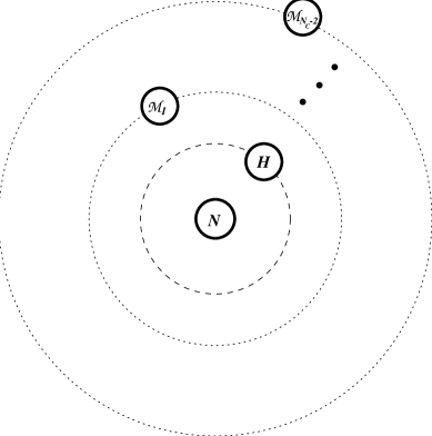
FIG. 1.: Schematic planetary picture for large $N_{\rm C}$ excited heavy baryons in the bound state approach.

One might imagine a number of different schemes for treating the inevitably complicated bound state dynamics of such a system. Even in the $N_{\rm C}=3$ case it is much simpler if we can manage to reduce the three body problem to an effective two body problem. This can be achieved, as schematically indicated in Fig. 2, if we link the two “orbiting” mesons together in a state which carries internal angular momentum.

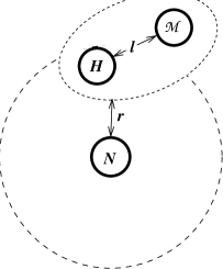
FIG. 2.: Schematic picture of the “two body” approximation for the $N_{\rm C}=3$ excited heavy baryons.

The “linked mesons” will be described mathematically by a single excited heavy meson multiplet field. One may alternatively consider these “linked mesons” as bare heavy mesons surrounded by a light meson cloud. Such fields are usually classified by the value, $\ell$ of the relative orbital angular momentum of a $\bar{q}Q$ pair which describes it in the CQM. We will not attempt to explain the binding of these two mesons but shall simply incorporate the “experimental” higher spin meson fields into our chiral Lagrangian. Different $\ell$ excitations will correspond to the use of different meson field multiplets. From now on we will restrict our attention to $N_{\rm C}=3$.

Taking the new degree of freedom $\ell$ into account requires us to modify the previous formulas describing the heavy baryon. Now the parity formula (25) is modified to

$$P_{B}=\left(-1\right)^{\ell+r}\ ,$$ (36)

which is seen to be compatible with the CQM relation (2). Now Eq. (31) holds but with the light grand spin $g$ modified to,

$$\mbox{\boldmath$g$}=\mbox{\boldmath$r$}+\mbox{\boldmath$K^{\prime}$}\ .$$ (37)

Note that $K$ in Eq. (18) has been incorporated in

$$\mbox{\boldmath$K^{\prime}$}=\mbox{\boldmath$I$}_{\rm light}+\mbox{\boldmath$S$}_{\rm light}+\mbox{\boldmath$\ell$}\ .$$ (38)

The new correspondence between the bound–state picture variables and those of the CQM is:

$$\mbox{\boldmath$S$}_{\rm heavy} \leftrightarrow \mbox{\boldmath$S$}_{H}\ ,$$ (39)

$$r \leftrightarrow \mbox{\boldmath$L$}_{E}\ ,$$ (40)

$$\ell \leftrightarrow \mbox{\boldmath$L$}_{I}\ ,$$ (41)

$$\mbox{\boldmath$I$}_{\rm light}+\mbox{\boldmath$S$}_{\rm light}+\mbox{\boldmath$J$}^{\rm sol} \leftrightarrow \mbox{\boldmath$S$}\ .$$ (42)

Previously $\mbox{\boldmath$I$}_{\rm light}+\mbox{\boldmath$S$}_{\rm light}=\mbox{\boldmath$K$}$ had zero quantum numbers on the bound states; now the picture is a little more complicated. We will see that the dynamics may lead to new bound states which are in correspondence with the CQM. Equation (42) should be interpreted in the sense of this correspondence.

It is easiest to see that the lowest new states generated agree with the CQM for $\ell=\mbox{even}$, which corresponds to negative parity heavy mesons. In this case $k=0$ or equivalently $k^{\prime}=\ell$ may be favored dynamically. Then the last line in Eq. (42) indicates that $J^{\rm sol}$, which can take on the values $0$ and $1$, corresponds to the light diquark spin $S$ in the CQM. This leads to the CQM states of type a) and b) in Eq. (6). This is just a generalization of the discussion for the ground state given in section II. Now let us discuss how the states corresponding to c) and d) can be constructed in the bound state scenario. Apparently we require $\ell=\mbox{odd}$, i.e. positive parity heavy mesons. For $I=0$ we also have $J^{\rm sol}=0$. Hence the last line in Eq. (42) requires $k=1$ for $S=1$. To generate states of type d) also $k=1$ would be needed in order to accommodate $I=J^{\rm sol}=1$ and $S=0$. Actually for the case $k=1$ and $J^{\rm sol}=1$ states with $S=0,1,2$ would be possible. The states with $S=1,2$ should be ruled out by the dynamics of the model.

One may perhaps wonder whether we are pushing the bound state picture too far; since things seen to be getting more complicated why not just use the constituent quark model? Apart from the intrinsic interest of the soliton approach there are two more or less practical reasons for pursuing the approach. The first is that the parameters of the underlying chiral Lagrangian are, unlike parameters such as the constituent quark masses and inter–quark potentials of the CQM, physical ones and in principle subject to direct experimental test. The second reason is that the bound state approach actually models the expected behavior of a confining theory; namely, when sufficient energy is applied to “stretch” the heavy baryon it does not come apart into a heavy quark and two light quarks but rather into a nucleon and a heavy meson. The light quark–antiquark pair which one usually imagines popping out of the vacuum when the color singlet state has been suitably stretched, was there all the time, waiting to play a role, in the bound state picture. The model may therefore be useful in treating reactions of this sort.

IV A model for the missing first excited states

Before going on to the general orbital excited states it may be helpful to see how the dynamics could work out for explaining the missing seven $\Lambda_{Q}$ and $\Sigma_{Q}$ type, negative parity, excited states. In the new bound state picture these correspond to the choices $\ell=1$, $r=0$. As discussed, we are considering that the orbital angular momentum $\ell$ is “locked–up” in suitable excited heavy mesons. As in Eq. (17), $r$ appears as a parameter in the new heavy meson wave–function. The treatment of the excited heavy mesons in the effective theory context, has been given already by Falk and Luke [21]. For a review see [22]. The case (for orbital angular momentum=1) where the light cloud spin of the heavy meson is $1/2$ is described by the heavy multiplet

$${\cal{H}}=\frac{1-i\gamma_{\mu}V_{\mu}}{2}\left(S+i\gamma_{5}\gamma_{\nu}A_{\nu}\right)\ ,$$ (43)

where $S$ is the fluctuation field for a scalar ($J^{P}=0^{+}$) particle and $A_{\mu}$, satisfying $V_{\mu}A_{\mu}=0$, similarly corresponds to an axial ($J^{P}=1^{+}$) particle. The case where the light cloud spin is $3/2$ is described by

$${\cal{H_{\mu}}}=\frac{1-i\gamma_{\alpha}V_{\alpha}}{2}\left(-T_{\mu\nu}\gamma_{\nu}+i\sqrt{\frac{3}{2}}B_{\nu}\gamma_{5}\left[\delta_{\mu\nu}-\frac{1}{3}\gamma_{\nu}\left(\gamma_{\mu}+iV_{\mu}\right)\right]\right)$$ (44)

satisfying the Rarita-Schwinger constraints ${\cal H}_{\mu}\gamma_{\mu}={\cal H}_{\mu}V_{\mu}=0$. The field $T_{\mu\nu}=T_{\nu\mu}$ (with $V_{\mu}T_{\mu\nu}=T_{\mu\mu}=0$) is a spin $2$ tensor ($J^{P}=2^{+}$) and $B_{\mu}$ (with $V_{\mu}B_{\mu}=0$) is another axial ($J^{P}=1^{+}$). Currently, experimental candidates exist for the tensor and an axial.

In order to prevent the calculation from becoming too complicated we will, for the purpose of the present paper, adopt the approximation of leaving out the light vector mesons. This is a common approximation used by workers in the field but it should be kept in mind that the effect of the light vectors is expected to be substantial.

The kinetic terms of the effective chiral Lagrangian (analogous to the first term of Eq. (14)) are:

$${\cal L}_{\rm kin}=-i{\cal M}V_{\mu}\mbox{Tr}\,\left[{\cal H}D_{\mu}\bar{{\cal H}}\right]+i{\cal M}\,V_{\mu}\mbox{Tr}\,\left[{\cal H}_{\mu}D_{\mu}\bar{\cal H}_{\mu}\right]\ ,$$ (45)

where ${\cal M}$ is a characteristic heavy mass scale for the excited mesons. For simplicity we are neglecting mass differences between the $\ell=1$ heavy mesons. The interaction terms involving only the ${\cal H}$ and ${\cal H}_{\mu}$ fields, to lowest order in derivatives, are

$${\cal L}_{\rm int}/{\cal M} = id_{\rm S}\mbox{Tr}\,\left[{\cal H}\gamma_{\mu}\gamma_{5}p_{\mu}\bar{\cal H}\right]-id_{\rm T}\mbox{Tr}\,\left[{\cal H}_{\mu}\gamma_{\alpha}\gamma_{5}p_{\alpha}\bar{\cal H}_{\mu}\right]$$ (46)

$$+ \left[if_{\rm ST}\mbox{Tr}\,\left[{\cal H}\gamma_{5}p_{\mu}\bar{\cal H}_{\mu}\right]+\mbox{h.c.}\right]\ .$$ (47)

These generalize the second term in Eq. (14) and $d_{\rm S}$, $d_{\rm T}$ and $f_{\rm ST}$ (which may be complex) are the heavy meson–pion coupling constants. Similar terms which involve $\ell\neq 1$ multiplets are not needed for our present purpose but will be discussed in the next section.

As in section II, the wave–functions for the excited heavy mesons bound to the background Skyrmion are conveniently presented in the rest frame $\mbox{\boldmath$V$}=0$. The analogs of Eq. (15) become

$$\bar{{\cal H}}_{\rm c}\rightarrow\left(\begin{array}[]{cc}\bar{f}_{lh}^{a}&0\\ 0&0\end{array}\right)\ ,\quad\left(\bar{{\cal H}}_{i}\right)_{\rm c}\rightarrow\left(\begin{array}[]{cc}0&0\\ \bar{f}_{i,lh}^{a}&0\end{array}\right)\ ,$$ (48)

and $\left(\bar{{\cal H}}_{0}\right)_{\rm c}\rightarrow 0$. Now the wave–functions in Eq. (48) are expanded as:

$$\bar{f}_{lh}^{a} = \frac{u\left(|\mbox{\boldmath$x$}|\right)}{\sqrt{{\cal M}}}\left(\hat{\mbox{\boldmath$x$}}\cdot\mbox{\boldmath$\tau$}_{ad}\right)\Phi_{ld}\left(k^{\prime},k^{\prime}_{3};r\right)\chi_{h}\ ,$$ (49)

$$\bar{f}_{i,lh}^{a} = \frac{u\left(|\mbox{\boldmath$x$}|\right)}{\sqrt{{\cal M}}}\left(\hat{\mbox{\boldmath$x$}}\cdot\mbox{\boldmath$\tau$}_{ad}\right)\Phi_{i,ld}\left(k^{\prime},k^{\prime}_{3};r\right)\chi_{h}\ ,$$ (50)

where $u$ stands for a sharply peaked radial wave–function which may differ for the two cases. Other notations are as in Eq. (16). Note that the constraint $\gamma_{\mu}\bar{\cal H}_{\mu}=0$ implies that

$$\left(\sigma_{i}\right)_{ll^{\prime}}\Phi_{i,l^{\prime}d}=0\ .$$ (51)

It is interesting to see explicitly how the extra angular momentum $\ell=1$ is “locked–up” in the heavy meson wave–functions. For the ${\cal H}$ wave–function, the fact that $\mbox{\boldmath$J$}_{\rm light}=\mbox{\boldmath$\ell$}+\mbox{\boldmath$S$}_{\rm light}$ takes the value $1/2$ leads, using Eq. (38), to the possible values $k^{\prime}=0$ or $1$. The corresponding wave–functions are

$$\Phi_{ld}\left(k^{\prime}=k^{\prime}_{3}=0\right)=\frac{\epsilon_{ld}}{\sqrt{8\pi}}\ ,\quad\Phi_{ld}\left(k^{\prime}=k_{3}=1\right)=\frac{\delta_{l1}\delta_{d1}}{\sqrt{4\pi}}\ ,$$ (52)

where, for the present case, we are taking $r=0$. For the $\bar{\cal H}_{i}$ wave–function it is important to satisfy $j_{l}=|\mbox{\boldmath$J$}_{\rm light}|$ = $3/2$ condition (51). This may be accomplished by combining with suitable Clebsch-Gordan coefficients an $\ell=1$ wave–function with the $S_{\rm light}=1/2$ spinor to give

$$\Phi_{i,ld}\left(k^{\prime}=k^{\prime}_{3}=2\right) = w^{(+1)}_{i}\delta_{l1}\delta_{d1}\ ,$$ (53)

$$\Phi_{i,ld}\left(k^{\prime}=k^{\prime}_{3}=1\right) = \frac{\sqrt{3}}{2}w^{(+1)}_{i}\delta_{l1}\delta_{d2}-\frac{1}{2\sqrt{3}}w^{(+1)}_{i}\delta_{l2}\delta_{d1}-\frac{1}{\sqrt{6}}w^{(0)}_{i}\delta_{l1}\delta_{d1}\ ,$$ (54)

where $w^{(\pm 1)}_{j}=\frac{\mp 1}{\sqrt{8\pi}}\left(\delta_{j1}\pm i\delta_{j2}\right)$ and $w^{(0)}_{i}=\frac{\delta_{i3}}{\sqrt{4\pi}}$ is a spherical decomposition.

The main question is: Which of the channels contain bound states? Note that, for the reduced space in which $\hat{\mbox{\boldmath$x$}}\cdot\mbox{\boldmath$\tau$}$ has been removed as in Eq. (50), $k^{\prime}$ is a good quantum number. Furthermore, because the wave–function $u\left(|\mbox{\boldmath$x$}|\right)$ is sharply peaked, the relevant matrix elements are actually independent of the orbital angular momentum $r$. The classical potential for each $k^{\prime}$ channel may be calculated by setting $r=0$ and substituting the appropriate reduced wave–functions from Eqs. (52) and (54) into the interaction Lagrangian (47). (see Appendix A for more details.) The $k^{\prime}=0$ channel gets a contribution only from the $d_{\rm S}$ term in Eq. (47) while the $k^{\prime}=2$ channel receives a contribution only from the $d_{\rm T}$ term. On the other hand, all three terms contribute to the $k^{\prime}=1$ channel. The resulting potentials are:

$$V\left(k^{\prime}=0\right) = -\frac{3}{2}d_{\rm S}F^{\prime}(0)\ ,$$ (55)

$$V\left(k^{\prime}=2\right) = -\frac{1}{2}d_{\rm T}F^{\prime}(0)\ ,$$ (56)

$$V\left(k^{\prime}=1\right)=\left(\begin{array}[]{cc}\langle{\cal H}|V|{\cal H}\rangle&\langle{\cal H}|V|{\cal H}_{\mu}\rangle\\ \langle{\cal H}_{\mu}|V|{\cal H}\rangle&\langle{\cal H}_{\mu}|V|{\cal H}_{\mu}\rangle\end{array}\right)=\left(\begin{array}[]{cc}\frac{1}{2}d_{\rm S}&-i\sqrt{\frac{2}{3}}f_{\rm ST}\\ i\sqrt{\frac{2}{3}}f_{\rm ST}^{*}&\frac{5}{6}d_{\rm T}\end{array}\right)F^{\prime}(0)\ .$$ (57)

The classical criterion for a channel to contain a bound state is that its potential be negative. Since $F^{\prime}(0)>0$ we require for bound states in the $k^{\prime}=0$ and $k^{\prime}=2$ channels

$$d_{\rm S}>0\ ,\quad d_{\rm T}>0\ ,$$ (58)

respectively. For bound states in the $k^{\prime}=1$ channel we must examine the signs of the eigenvalues of Eq. (57). Assuming that Eq. (58) holds (as will be seen to be desirable) it is easy to see that there is, at most, one $k^{\prime}=1$ bound state. The condition for this bound state to exist is

$$\left|{f_{\rm ST}}\right|^{2}>\frac{5}{8}\,d_{S}\,d_{T}\ .$$ (59)

The (primed) states which diagonalize Eq. (57) are simply related to the original ones by

$$\left(\begin{array}[]{c}\Phi\\ \Phi_{i}\end{array}\right)=\left(\begin{array}[]{cc}\cos\theta&\sin\theta\\ -ip^{*}\sin\theta&ip\cos\theta\end{array}\right)\left(\begin{array}[]{c}\Phi^{\prime}\\ \Phi_{i}^{\prime}\end{array}\right)\ ,$$ (60)

$$\tan 2\theta=\frac{4\sqrt{6}\left|f_{\rm ST}\right|}{5d_{\rm T}-3d_{\rm S}}\ ,$$ (61)

where $p$ is the phase of $f_{\rm ST}$. $\Phi$ and $\Phi_{i}$ are shorthand notations for the appropriate wave–functions. Clearly, the results for which states are bound depend on the numerical values and signs of the coupling constants. At the moment there is no purely experimental information on these quantities. However, it is very interesting to observe that if Eqs. (58) and (59) hold, then the missing first excited $\Lambda_{Q}$ states are bound. To see this note that the heavy baryon spin is given by Eq. (31) with $g$ defined in Eqs. (37) and (38). For the $\Lambda_{Q}$–type states, noting that $I=J^{\rm sol}=0$ in the Skyrme approach gives the baryon spin as

$$\mbox{\boldmath$J$}=\mbox{\boldmath$g$}+\mbox{\boldmath$S$}_{\rm heavy}\quad\left(\Lambda_{Q}~{}{\rm states}\right)\ .$$ (62)

The $r=0$ choice enables us to set $g=k^{\prime}$. With just the three attractive channels $k^{\prime}=0$, $k^{\prime}=1$ and $k^{\prime}=2$ we thus end up with the missing first three excited $\Lambda_{Q}$ heavy multiplets $\Lambda_{Q}\left(\frac{1}{2}^{-}\right)$ , $\left\{\Lambda_{Q}\left(\frac{1}{2}^{-}\right),\Lambda_{Q}\left(\frac{3}{2}^{-}\right)\right\}$ and $\left\{\Lambda_{Q}\left(\frac{3}{2}^{-}\right),\Lambda_{Q}\left(\frac{5}{2}^{-}\right)\right\}$. It should be stressed that this counting involves dynamics rather than pure kinematics. For example, it may be seen from Eqs. (55)–(57) that it is dynamically impossible to have four bound heavy multiplets ($k^{\prime}=0,~{}k^{\prime}=2$ and two $k^{\prime}=1$ channels). The missing first excited $\Sigma_{Q}$–type states comprise the single heavy multiplet $\left\{\Sigma_{Q}\left(\frac{1}{2}^{-}\right),\Sigma_{Q}\left(\frac{3}{2}^{-}\right)\right\}$. At the classical level there are apparently more bound multiplets present. However, we will now see that the introduction of collective coordinates, as is anyway required in the Skyrme model [23] to generate states with good isospin quantum number, will split the heavy multiplets from each other. Thus, deciding which states are bound actually requires a more detailed analysis.

We need to extend Eq.. (28) in order to allow the $\ell=1$ heavy meson fields to depend on the collective rotation variable $A(t)$:

$$\bar{{\cal H}}(\mbox{\boldmath$x$},t)=A(t)\bar{{\cal H}}_{\rm c}(\mbox{\boldmath$x$})\ ,\quad\bar{{\cal H}}_{i}(\mbox{\boldmath$x$},t)=A(t)\bar{{\cal H}}_{i{\rm c}}(\mbox{\boldmath$x$})\ ,$$ (63)

where $\bar{{\cal H}}_{\rm c}$ and $\bar{{\cal H}}_{i{\rm c}}$ are given in Eq. (48). Note, again, that the matrix $A(t)$ acts on the isospin indices. We also have $\bar{{\cal H}}_{0{\rm c}}=0$ due to the rest frame constraint $V_{\mu}\bar{{\cal H}}_{\mu{\rm c}}=0$. Now substituting Eq. (63) as well as the first of Eq. (28) into the heavy field Lagrangian yields [1] the collective Lagrangian

$$L_{\rm coll}=\frac{1}{2}\,\alpha^{2}\mbox{\boldmath$\Omega$}^{2}-\chi\left(k^{\prime}\right)\mbox{\boldmath$K^{\prime}$}\cdot\mbox{\boldmath$\Omega$}\ ,$$ (64)

where $\Omega$ is defined in Eq. (29) and $\alpha^{2}$ is the Skyrme model moment of inertia. In the vector meson model the induced fields ($\rho^{a}_{0}$ and $\omega_{i}$) are determined from a variational approach to $\alpha^{2}$. The quantities $\chi\left(k^{\prime}\right)$ are given by (see Appendix B).

$$\chi\left(k^{\prime}\right)=\left\{\begin{array}[]{ll}0&k^{\prime}=0\\ \frac{1}{4}\left(3\,\cos^{2}\theta-1\right)&k^{\prime}=1\\ \frac{1}{4}&k^{\prime}=2\end{array}\right.\ ,$$ (65)

where the angle $\theta$ is defined in Eq. (61). (Note that if light vector mesons are included the expressions for $\chi$ would be more involved as the induced fields will also contribute.) In writing Eq. (65) it was assumed that the first state in Eq. (60) (i.e. $\Phi^{\prime}$ rather than $\Phi^{\prime}_{i}$) is the bound one; the collective Lagrangian is constructed as an expansion around the bound state solutions. We next determine from Eq. (30), the canonical (angular) momentum $\mbox{\boldmath$J$}^{\rm sol}$ as $\alpha^{2}\,\mbox{\boldmath$\Omega$}-\chi\left(k^{\prime}\right)\mbox{\boldmath$K$}^{\prime}$. The usual Legendre transform then leads to the collective Hamiltonian

$$H_{\rm coll}=\frac{1}{2\alpha^{2}}\left(\mbox{\boldmath$J$}^{\rm sol}+\chi\left(k^{\prime}\right)\,\mbox{\boldmath$K^{\prime}$}\right)^{2}\ .$$ (66)

Again we remark that $J^{\rm sol}=I$. It is useful to define the light part of the total heavy baryon spin as

$$\mbox{\boldmath$j$}=\mbox{\boldmath$r$}+\mbox{\boldmath$K$}^{\prime}+\mbox{\boldmath$J$}^{\rm sol}\ ,$$ (67)

and rewrite Eq. (66) as

$$H_{\rm coll}=\frac{1}{2\alpha^{2}}\left[\left(1-\chi\left(k^{\prime}\right)\right)\mbox{\boldmath$I$}^{2}+\chi\left(k^{\prime}\right)\left(\mbox{\boldmath$j$}-\mbox{\boldmath$r$}\right)^{2}+\chi\left(k^{\prime}\right)\left(\chi\left(k^{\prime}\right)-1\right)\mbox{\boldmath$K^{\prime}$}^{2}\right]\ .$$ (68)

The mass splittings within each given $k^{\prime}$ multiplet due to $H_{\rm coll}$ are displayed in Table II.

$I$	$k^{\prime}$	$\left|\mbox{\boldmath$K$}^{\prime}+\mbox{\boldmath$J$}^{\rm sol}\right|$	$V$	$\alpha^{2}H_{\rm coll}$	Candidates for $r=0$
$=J^{\rm sol}$					missing states
	0	0	$-\frac{3}{2}d_{\rm S}\,F^{\prime}(0)$	0	$\Lambda_{Q}\left(\frac{1}{2}^{-}\right)$
0	1	1	$\lambda$	$\chi^{2}$	$\left\{\Lambda_{Q}\left(\frac{1}{2}^{-}\right),\Lambda_{Q}\left(\frac{3}{2}^{-}\right)\right\}$
	2	2	$-\frac{1}{2}d_{\rm T}\,F^{\prime}(0)$	$\frac{3}{16}$	$\left\{\Lambda_{Q}\left(\frac{3}{2}^{-}\right),\Lambda_{Q}\left(\frac{5}{2}^{-}\right)\right\}$
	0	1	$-\frac{3}{2}d_{\rm S}\,F^{\prime}(0)$	1	$\left\{\Sigma_{Q}\left(\frac{1}{2}^{-}\right),\Sigma^{\prime}_{Q}\left(\frac{3}{2}^{-}\right)\right\}_{1}$
	1	0	$\lambda$	$\left(\chi-1\right)^{2}$
	1	1	′′	$\left(\chi-1\right)^{2}+\chi$	$\left\{\Sigma_{Q}\left(\frac{1}{2}^{-}\right),\Sigma_{Q}\left(\frac{3}{2}^{-}\right)\right\}_{2}$
1	1	2	′′	$\left(\chi-1\right)^{2}+3\,\chi$
	2	1	$-\frac{1}{2}d_{\rm T}\,F^{\prime}(0)$	$\frac{7}{16}$	$\left\{\Sigma_{Q}\left(\frac{1}{2}^{-}\right),\Sigma_{Q}\left(\frac{3}{2}^{-}\right)\right\}_{3}$
	2	2	′′	$\frac{15}{16}$
	2	3	′′	$\frac{27}{16}$

TABLE II.: Contributions to energies of new predicted $\ell=1$ states. Here, $\lambda=\frac{1}{4}F^{\prime}(0)\left[\left(d_{\rm S}+\frac{5}{3}d_{\rm T}\right)-\sqrt{\left(d_{\rm S}-\frac{5}{3}d_{\rm T}\right)^{2}+\frac{32}{3}|f_{\rm ST}|^{2}}\right]$ is the presumed negative binding potential in the $k^{\prime}=1$ channel. Furthermore $\chi=\chi(1)$ in Eq. (65); it satisfies $-\frac{1}{4}\leq\chi\leq\frac{1}{2}$.

This table also shows the splitting of the $k^{\prime}$ multiplets from each other due to the classical potential in Eqs. (55)–(57). Note that the slope of the Skyrme profile function $F^{\prime}(0)$ is of order $1$ GeV. The coupling constants $d_{\rm S},d_{\rm T},f_{\rm ST}$, based on $d\simeq 0.5$ for the ground state heavy meson, are expected to be of the order unity. Hence the binding potentials $V$ are expected to be of the rough order of $500$ MeV. The inverse moment of inertia $1/\alpha^{2}$ is of the order of $200$ MeV which (together with $-\frac{1}{4}\leq\chi\leq\frac{1}{2}$) sets the scale for the “$1/N_{\rm C}$” corrections due to $H_{\rm coll}$. As mentioned before, if the coupling constants satisfy the inequalities (58) and (59), all the $\Lambda_{Q}$ multiplets shown will be bound. At first glance we might expect all the $\Sigma_{Q}$ states listed also to be bound. However the $H_{\rm coll}$ corrections increase as $I$ increases, which is a possible indication that many of the $\Sigma_{Q}$’s might be only weakly bound. In a more complete model they may become unbound. Hence it is interesting to ask which of the three displayed candidates for the single missing $\Sigma_{Q}$ multiplet is mostly tightly bound in the present model. Neglecting the effect of $V$ we can see that $H_{\rm coll}$ raises the energy of candidate 3 less than those of candidates 1 and 2. Furthermore, for the large range of $\chi$, $-\frac{1}{4}\leq\chi\leq 1-\frac{\sqrt{7}}{4}$, candidate 3 suffers the least unbinding due to $H_{\rm coll}$ of any of the $I=1$ heavy baryons listed. The $\Lambda_{Q}$ states suffer still less unbinding due to $H_{\rm coll}$.

V Higher Orbital Excitations

We have already explicitly seen that the “missing” first orbitally excited heavy baryon states in the bound state picture might be generated if the model is extended to also include binding the first orbitally excited heavy mesons in the background field of a Skyrme soliton. From the correspondence (42) and associated discussion we expect that any of the higher excited heavy baryons of the CQM might be similarly generated by binding the appropriately excited heavy mesons. In this section we will show in detail how this result can be achieved in the general case. An extra complication, which was neglected for simplicity in the last section, is the possibility of baryon states constructed by binding heavy mesons of different $\ell$, mixing with each other. For example $\{r=1\,,\,\ell=0\}$ type states can mix with $\{r=1\,,\,\ell=2\}$ type states, other quantum numbers being the same. Since $\mbox{\boldmath$r$}+\mbox{\boldmath$\ell$}$ must add to $1$, this channel could not mix with $\{r=1\,,\,\ell=4\}$. An identical type of mixing – between $\{L_{E}=1\,,\,L_{I}=0\}$ and $\{L_{E}=1\,,\,L_{I}=2\}$ – may also exist in the CQM. The present model, however, provides a simple way to study this kind of mixing as a perturbation.

field	$\ell$	$j_{l}$	$J^{P}$
$H$	0	$1/2$	$0^{-}$, $1^{-}$
${\cal H}$	1	$1/2$	$0^{+}$, $1^{+}$
${\cal H}_{\mu}$	1	$3/2$	$1^{+}$, $2^{+}$
$H_{\mu}$	2	$3/2$	$1^{-}$, $2^{-}$
$H_{\mu\nu}$	2	$5/2$	$2^{-}$, $3^{-}$
⋮
$H_{\mu_{1}\cdots\mu_{\ell-1}}$	$\ell=\mbox{even}$	$\ell-1/2$	$(\ell-1)^{-}$, $\ell^{-}$
$H_{\mu_{1}\cdots\mu_{\ell}}$	$\ell=\mbox{even}$	$\ell+1/2$	$\ell^{-}$, $(\ell+1)^{-}$
${\cal H}_{\mu_{1}\cdots\mu_{\ell-1}}$	$\ell=\mbox{odd}$	$\ell-1/2$	$(\ell-1)^{+}$, $\ell^{+}$
${\cal H}_{\mu_{1}\cdots\mu_{\ell}}$	$\ell=\mbox{odd}$	$\ell+1/2$	$\ell^{+}$, $(\ell+1)^{+}$
⋮

TABLE III.: Notation for the heavy meson multiplets. $j_{l}$ is the angular momentum of the “light cloud” surrounding the heavy quark while $J^{P}$ is the spin parity of each heavy meson in the multiplet.

To start the analysis it may be helpful to refer to Table III, which shows our notations for the excited heavy meson multiplet “fluctuation” fields. The straight $H$’s contain negative parity mesons and the curly ${\cal H}$’s contain positive parity mesons. Further details are given in Ref. [21]. Note that each field is symmetric in all Lorentz indices and obeys the constraints

$$V_{\mu_{1}}H_{\mu_{1}\cdots\mu_{n}}=H_{\mu_{1}\cdots\mu_{n}}\gamma_{\mu_{1}}=0\ ,$$ (69)

as well as for ${\cal H}_{\mu_{1}\cdots\mu_{n}}$. The general chiral invariant interaction with the lowest number of derivatives is

$${\cal L}_{\rm d}+{\cal L}_{\rm f}+{\cal L}_{\rm g}\ ,$$ (70)

where

$${\cal L}_{\rm d} = iM\sum_{n=0}d_{{\rm P}n}\left(-1\right)^{n}\mbox{\rm Tr}\,\left[H_{\mu_{1}\cdots\mu_{n}}p_{\mu}\gamma_{\mu}\gamma_{5}\bar{H}_{\mu_{1}\cdots\mu_{n}}\right]$$ (72)

$${}+iM\sum_{n=0}d_{{\rm S}n}\left(-1\right)^{n}\mbox{\rm Tr}\,\left[{\cal H}_{\mu_{1}\cdots\mu_{n}}p_{\mu}\gamma_{\mu}\gamma_{5}\bar{\cal H}_{\mu_{1}\cdots\mu_{n}}\right]\ ,$$

$${\cal L}_{\rm f} = iM\sum_{n=0}f_{{\rm P}n}\left(-1\right)^{n}\mbox{\rm Tr}\,\left[H_{\mu_{1}\cdots\mu_{n}}p_{\mu}\gamma_{5}\bar{H}_{\mu_{1}\cdots\mu_{n}\mu}\right]+\mbox{h.c.}$$ (74)

$${}+iM\sum_{n=0}f_{{\rm S}n}\left(-1\right)^{n}\mbox{\rm Tr}\,\left[{\cal H}_{\mu_{1}\cdots\mu_{n}}p_{\mu}\gamma_{5}\bar{\cal H}_{\mu_{1}\cdots\mu_{n}\mu}\right]+\mbox{h.c.}\ .$$

The final piece,

$${\cal L}_{\rm g}=iM\sum_{n=0}g_{n}\left(-1\right)^{n}\mbox{\rm Tr}\,\left[{\cal H}_{\mu_{1}\cdots\mu_{n}}p_{\mu}\gamma_{\mu}\gamma_{5}\bar{H}_{\mu_{1}\cdots\mu_{n}}\right]+\mbox{h.c.}$$ (75)

exists in general, but does not contribute for our ansatz. Terms of the form

$$\mbox{\rm Tr}\,\left[H_{\mu_{1}\cdots\mu_{n}\mu}p_{\mu}\gamma_{5}\bar{\cal H}_{\mu_{1}\cdots\mu_{n}}\right]\ ,\qquad\mbox{\rm Tr}\,\left[{\cal H}_{\mu_{1}\cdots\mu_{n}\mu}p_{\mu}\gamma_{5}\bar{H}_{\mu_{1}\cdots\mu_{n}}\right]$$ (76)

can be shown to vanish by the heavy spin symmetry. In the notation of Eq. (47), $d_{\rm S}=d_{{\rm S}0}$, $d_{\rm T}=d_{{\rm S}1}$ and $f_{\rm ST}=f_{{\rm S}0}$. A new type of coupling present in Eq. (74) also connects multiplets to others differing by $\Delta\ell=\pm 2$. These are the terms with odd (even) $n$ for $H$ (${\cal H}$)–type fields. The interactions in Eq. (75) connecting multiplets differing by $\Delta\ell=\pm 1$ turn out not to contribute in our model. In the interest of simplicity we will consider all heavy mesons to have the same mass. This is clearly an approximation which may be improved in the future.

The rest frame ansätze for the bound state wave functions which generalize Eq. (48) are (note $j_{l}=n+1/2$):

$$\left(\bar{H}_{i_{1}\cdots i_{n}}\right)_{\rm c}\rightarrow\left\{\begin{array}[]{l}\displaystyle\bar{h}^{a}_{i_{1}\cdots i_{n},lh}\otimes\left(\begin{array}[]{cc}0&0\\ 1&0\end{array}\right)\ ,\qquad j_{l}=\ell+\frac{1}{2}\ ,\\ \displaystyle\bar{h}^{a}_{i_{1}\cdots i_{n},lh}\otimes\left(\begin{array}[]{cc}1&0\\ 0&0\end{array}\right)\ ,\qquad j_{l}=\ell-\frac{1}{2}\ ,\end{array}\right.$$ (77)

with identical structures for $\bar{H}\rightarrow\bar{\cal H}$. Note that again $a$, $l$, $h$ represent respectively the isospin, light spin and heavy spin bivalent indices. Extracting a factor of $\hat{\mbox{\boldmath$x$}}\cdot\mbox{\boldmath$\tau$}$ as we did before in Eqs. (16) and (50) leads to

$$\bar{h}^{a}_{i_{1}\cdots i_{n},lh}=\frac{u\left(\left|\mbox{\boldmath$x$}\right|\right)}{\sqrt{M}}\left(\hat{\mbox{\boldmath$x$}}\cdot\mbox{\boldmath$\tau$}\right)_{ad}\psi_{i_{1}\cdots i_{n},dl}\left(k^{\prime},k_{3}^{\prime},r\right)\,\chi_{h}$$ (78)

with similar notations. The relevant wave–functions are the $\psi_{i_{1}\cdots i_{n},dl}\left(k^{\prime},k_{3}^{\prime},r\right)$. $k^{\prime}$ was defined in Eq. (38); we will see that it remains a good quantum number. Since the terms which connect the positive parity ($H$ type) and negative parity (${\cal H}$ type) heavy mesons (Eq. (75)) vanish when the ansätze (77) are substituted, the baryon states associated with each type do not mix with each other in our model. We thus list separately the potentials for each type. For the $\ell=\mbox{even}$ baryons (associated with $H$ mesons),

$$V\left[k^{\prime}=0\right] = -\frac{3}{2}d_{{\rm P}0}\,F^{\prime}(0)\ ,$$ (79)

$$V\left[k^{\prime}\neq 0\right] = F^{\prime}(0)\,\left[\begin{array}[]{cc}\displaystyle-\left(-1\right)^{k^{\prime}}\frac{d_{{\rm P}(k^{\prime}-1)}}{2}&\displaystyle-i\sqrt{\frac{2}{3}}f_{{\rm P}(k^{\prime}-1)}\\ \displaystyle i\sqrt{\frac{2}{3}}f^{\ast}_{{\rm P}(k^{\prime}-1)}&\displaystyle-\left(-1\right)^{k^{\prime}}\frac{2k^{\prime}+3}{2k^{\prime}+1}\frac{d_{{\rm P}k^{\prime}}}{2}\end{array}\right]\ ,$$ (82)

while for the $\ell=\mbox{odd}$ baryons (associated with ${\cal H}$ mesons),

$$V\left[k^{\prime}=0\right] = -\frac{3}{2}d_{{\rm S}0}\,F^{\prime}(0)\ ,$$ (83)

$$V\left[k^{\prime}\neq 0\right] = F^{\prime}(0)\,\left[\begin{array}[]{cc}\displaystyle-\left(-1\right)^{k^{\prime}}\frac{d_{{\rm S}(k^{\prime}-1)}}{2}&\displaystyle-i\sqrt{\frac{2}{3}}f_{{\rm S}(k^{\prime}-1)}\\ \displaystyle i\sqrt{\frac{2}{3}}f^{\ast}_{{\rm S}(k^{\prime}-1)}&\displaystyle-\left(-1\right)^{k^{\prime}}\frac{2k^{\prime}+3}{2k^{\prime}+1}\frac{d_{{\rm S}k^{\prime}}}{2}\end{array}\right]\ .$$ (86)

Details of the derivations of Eqs. (82) and (86) are given in Appendix A. The ordering of matrix elements in Eqs. (82) and (86), for a given $k^{\prime}$, is such that the first heavy meson has a light spin, $j_{l}=k^{\prime}-\frac{1}{2}$ while the second has $j_{l}=k^{\prime}+\frac{1}{2}$. The $H$ type (${\cal H}$ type) channels with $k^{\prime}=\mbox{even}$ (odd) involve two mesons with the same $\ell=k^{\prime}$. The $H$ type (${\cal H}$ type) channels with $k^{\prime}=\mbox{odd}$ (even) involve two mesons differing by $\Delta\ell=2$, i.e., $\ell=k^{\prime}-1$ and $\ell=k^{\prime}+1$. This pattern is, for convenience, illustrated in Table IV.

		$H$ mesons		${\cal H}$ mesons
$k^{\prime}$	$j_{l}$	$\ell$	#	$\ell$	#
$0$	$1/2$	$0$	$1$	$1$	$1$
$1$	$\begin{array}[]{c}$1/2$\\ $3/2$\end{array}$	$\begin{array}[]{c}$0$\\ $2$\end{array}$	$0$	$\begin{array}[]{c}$1$\\ $1$\end{array}$	1
$2$	$\begin{array}[]{c}$3/2$\\ $5/2$\end{array}$	$\begin{array}[]{c}$2$\\ $2$\end{array}$	$1$	$\begin{array}[]{c}$1$\\ $3$\end{array}$	2
$3$	$\begin{array}[]{c}$5/2$\\ $7/2$\end{array}$	$\begin{array}[]{c}$2$\\ $4$\end{array}$	$0$	$\begin{array}[]{c}$3$\\ $3$\end{array}$	1

TABLE IV.: Pattern of states for Eqs. (82) and (86). Note that $j_{l}=n+\frac{1}{2}$ is the light cloud spin of the heavy meson. The columns marked # stand for the number of channels which are expected to be bound, for that particular $k^{\prime}$, according to the CQM.

Also shown, for each $k^{\prime}$, are the number of channels which are expected to be bound according to the CQM.

It is important to note that Table IV holds for any value of the angular momentum $r$, which is a good quantum number in our model. For the reader’s orientation, we now locate the previously considered cases in Table IV. The standard “ground state” heavy baryons discussed in section II are made from the $H$ meson with $\ell=0$ and $j_{l}=1/2$. They have $r=0$ and $k^{\prime}=0$. The seven negative parity heavy baryons discussed in section II also are made from the $H$ meson with $\ell=0$ and $j_{l}=1/2$. They still have $k^{\prime}=0$, but now $r=1$. The seven “missing” first excited heavy baryons discussed in section IV have $r=0$ and are made from the $\ell=1$, ${\cal H}$ and ${\cal H}_{\mu}$ mesons with $j_{l}=1/2$ and $j_{l}=3/2$. There should appear one bound state for $k^{\prime}=0$, one bound state for $k^{\prime}=1$ and one bound state for $k^{\prime}=2$ in the “${\cal H}$–meson” section of Table IV. Note that the number of states expected in the CQM model for $k^{\prime}=2$ is listed in Table IV as two, rather than one. In the absence of $\Delta\ell=2$ terms connecting ${\cal H}_{\mu}$ and ${\cal H}_{\mu\nu}$ (see the last term in Eq. (74)) $\ell$ would be conserved for our model and only the $\ell=1$ state would be relevant. This was the approximation we made, for simplicity, in section IV. The other entry would have $\ell=3$ and would decouple. When the $\Delta\ell=2$ mixing terms are turned on, the $\ell=1$ and $\ell=3$, $k^{\prime}=2$ channels will mix. One diagonal linear combination should be counted against the $L_{I}=1$ CQM states and one against the $L_{I}=3$ CQM states.

To summarize: for the $H$–type mesons, the even $k^{\prime}$ channels should each have one bound state, while the odd $k^{\prime}$ channels should have none. The situation is very different for the ${\cal H}$–type mesons; then the even $k^{\prime}\neq 0$ channels should contain two bound states while the odd $k^{\prime}$ channels should contain one bound state. The $k^{\prime}=0$ channel should have one bound state.

For the $H$–type meson case, the pattern of bound states mentioned above would be achieved dynamically if the coupling constants satisfied:

$$d_{{\rm P}0}>0\ ,$$ (87)

$$\left(-1\right)^{k^{\prime}}\left[d_{{\rm P}(k^{\prime}-1)}d_{{\rm P}k^{\prime}}\left(\frac{2k^{\prime}+3}{2k^{\prime}+1}\right)-\frac{8}{3}\left|f_{{\rm P}(k^{\prime}-1)}\right|^{2}\right]<0\ ,\quad(k^{\prime}>0)$$ (88)

$$d_{{\rm P}(k^{\prime}-1)}+\left(\frac{2k^{\prime}+3}{2k^{\prime}+1}\right)d_{{\rm P}k^{\prime}}>0\ ,\quad(k^{\prime}=\mbox{odd})\ .$$ (89)

These follow from requiring only one negative eigenvalue of Eq. (82) for $k^{\prime}=\mbox{even}$ and none for $k^{\prime}=\mbox{odd}$. Similarly requiring for the ${\cal H}$–type meson case in Eq. (86), a negative eigenvalue for $k^{\prime}=0$, one negative eigenvalue for $k^{\prime}=\mbox{odd}$ and two negative eigenvalues for $k^{\prime}>0$ and even leads to the criteria,

$$d_{{\rm S}0}>0\ ,$$ (90)

$$\left(-1\right)^{k^{\prime}}\left[d_{{\rm S}(k^{\prime}-1)}d_{{\rm S}k^{\prime}}\left(\frac{2k^{\prime}+3}{2k^{\prime}+1}\right)-\frac{8}{3}\left|f_{{\rm S}(k^{\prime}-1)}\right|^{2}\right]>0\ ,\quad(k^{\prime}>0)$$ (91)

$$d_{{\rm S}(k^{\prime}-1)}+\left(\frac{2k^{\prime}+3}{2k^{\prime}+1}\right)d_{{\rm S}k^{\prime}}>0\ ,\quad(k^{\prime}=\mbox{even}\neq 0)\ .$$ (92)

From Eqs. (89) and (92) it can be seen that all the $d$’s are required to be positive. Furthermore these equations imply that the $\left|f\right|$’s which connect heavy mesons with $\Delta\ell=2$ are relatively small (compared to the $d$’s) while the $\left|f\right|$’s which connect heavy mesons with $\Delta\ell=0$ are relatively large. In detail this means that $\left|f_{{\rm P}(k^{\prime}-1)}\right|$ should be small for odd $k^{\prime}$ and large for even $k^{\prime}$ with just the reverse for $\left|f_{{\rm S}(k^{\prime}-1)}\right|$. This result seems physically reasonable.

As in the example in the preceding section we should introduce the collective variable $A(t)$ in order to define states of good isospin and angular momentum. This again yields some splitting of the different $\left|\mbox{\boldmath$K$}^{\prime}+\mbox{\boldmath$J$}^{\rm sol}\right|$ members of each $k^{\prime}$ bound state. Now, each $k^{\prime}$ channel (except for $k^{\prime}=0$) is described by a $2\times 2$ matrix. Thus there will be an appropriate mixing angle $\theta$, analogous to the one introduced in Eq. (60), for each $k^{\prime}$ and parity choice (i.e., $H$–type or ${\cal H}$–type field). The collective Lagrangian is still given by Eq. (64) but, in the general case,

$$\chi_{\pm}(k^{\prime})=\frac{1}{2k^{\prime}(k^{\prime}+1)}\left[\frac{1}{2}\pm\left(k^{\prime}+\frac{1}{2}\right)\cos 2\theta\right]\ .$$ (93)

In this formula the different signs corresponds to the two possible eigenvalues,

$$\lambda_{\pm}=\left[\frac{\left(-1\right)^{k^{\prime}-1}}{4}\left(d_{(k^{\prime}-1)}+\frac{2k^{\prime}+3}{2k^{\prime}+1}d_{k^{\prime}}\right)\pm\frac{1}{4}\sqrt{\left(d_{(k^{\prime}-1)}-\frac{2k^{\prime}+3}{2k^{\prime}+1}d_{k^{\prime}}\right)^{2}+\frac{32}{3}\left|f_{(k^{\prime}-1)}\right|^{2}}\right]F^{\prime}(0)$$ (94)

of the potential matrix. For example, referring to Table IV, we would expect the $k^{\prime}=2$, ${\cal H}$–type meson case to provide two distinct bound states and hence both $\chi_{+}(2,{\cal H})$ and $\chi_{-}(2,{\cal H})$ would be non-zero. On the other hand, we would expect no bound states in the $k^{\prime}=3$, $H$–type meson case so $\chi_{\pm}(3,H)$ should be interpreted as zero.

It is convenient to summarize the energies of the predicted states in tabular form, generalizing the example presented in Table II. The situation for baryons with $\mbox{parity}=-(-1)^{r}$ (${\cal H}$–type mesons) is presented in Table V. For definiteness we have made the assumption that the constraints (92) above are satisfied.

$I$	$k^{\prime}$	$\left|\mbox{\boldmath$K$}^{\prime}+\mbox{\boldmath$J$}^{\rm sol}\right|$	$V$	$\alpha^{2}\times H_{\rm coll}$	Candidates for $r=0$
$=J^{\rm sol}$					missing states
	$2n-1$	$2n-1$	$\lambda_{+}$	$n(2n-1)\chi_{-}^{2}$	$\left\{\Lambda\left((2n-3/2)^{-}\right)\,,\,\Lambda\left((2n-1/2)^{-}\right)\right\}$
$0$	$2n$	$2n$	$\lambda_{+}$	$n(2n+1)\chi_{+}^{2}$	$\left\{\Lambda\left((2n-1/2)^{-}\right)\,,\,\Lambda\left((2n+1/2)^{-}\right)\right\}$
			$\lambda_{-}$	$n(2n+1)\chi_{-}^{2}$	′′
	$2n-1$	$2n-2$		$n(2n-1)\chi_{+}^{2}+1-2n\chi_{+}$
		$2n-1$	$\lambda_{+}$	$n(2n-1)\chi_{+}^{2}+1-\chi_{+}$	$\left\{\Sigma\left((2n-3/2)^{-}\right)\,,\,\Sigma\left((2n-1/2)^{-}\right)\right\}_{1}$
		$2n$		$n(2n-1)\chi_{+}^{2}+1+(2n-1)\chi_{+}$
	$2n$	$2n-1$		$n(2n+1)\chi_{+}^{2}+1-(2n+1)\chi_{+}$	$\left\{\Sigma\left((2n-3/2)^{-}\right)\,,\,\Sigma\left((2n-1/2)^{-}\right)\right\}_{2}$
$1$		$2n$	$\lambda_{+}$	$n(2n+1)\chi_{+}^{2}+1-\chi_{+}$
		$2n+1$		$n(2n+1)\chi_{+}^{2}+1+2n\chi_{+}$	$\left\{\Sigma\left((2n+1/2)^{-}\right)\,,\,\Sigma\left((2n+3/2)^{-}\right)\right\}_{3}$
		$2n-1$		$n(2n+1)\chi_{-}^{2}+1-(2n+1)\chi_{-}$	$\left\{\Sigma\left((2n-3/2)^{-}\right)\,,\,\Sigma\left((2n-1/2)^{-}\right)\right\}_{4}$
		$2n$	$\lambda_{-}$	$n(2n+1)\chi_{-}^{2}+1-\chi_{-}$
		$2n+1$		$n(2n+1)\chi_{-}^{2}+1+2n\chi_{-}$	$\left\{\Sigma\left((2n+1/2)^{-}\right)\,,\,\Sigma\left((2n+3/2)^{-}\right)\right\}_{5}$

TABLE V.: Contributions to energies of the new predicted states made from ${\cal H}$–type heavy mesons. Note that $n$ is a positive integer. The $n=0$ case is given in Table II. The $\lambda_{+}$ entries in the $V$ column are more tightly bound than the $\lambda_{-}$ entries. $\left|\mbox{\boldmath$K$}^{\prime}+\mbox{\boldmath$J$}^{\rm sol}\right|$ is the light part of the heavy baryon angular momentum for $r=0$ (See Eq. (67).).

In order to explain Table V let us ask which states correspond to the ($L_{I}=3$, $L_{E}=0$) states in the CQM. Reference to Table I shows that three negative parity $\Lambda$–type heavy multiplets and one negative parity $\Sigma$–type heavy multiplet should be present. The correspondence in Eq. (42) instructs us to set $r=0$ and, noting Eq. (38) , to identify

$$\mbox{\boldmath$K$}^{\prime}+\mbox{\boldmath$J$}^{\rm sol}\leftrightarrow\mbox{\boldmath$L$}_{I}+\mbox{\boldmath$S$}\ .$$ (95)

The $\Lambda$–type particles are of type c) in Eq. (6) so we must take $S=1$. Hence, since $J^{\rm sol}=0$ for $\Lambda$–type particles, we learn that $k^{\prime}$ can take on the values $2$, $3$ and $4$. For $k^{\prime}=2$, the second line of the $k^{\prime}$ column yields two possible multiplets (energies $\lambda_{+}$ and $\lambda_{-}$) with $n=1$ and structure $\left\{\Lambda\left(\frac{3}{2}^{-}\right)\,,\,\Lambda\left(\frac{5}{2}^{-}\right)\right\}$. We should choose one of these to be associated with ($L_{I}=3$, $L_{E}=0$) and the other with ($L_{I}=1$, $L_{E}=0$) in the CQM. We remind the reader that $\ell$ is not a good quantum number so that the correspondence $\mbox{\boldmath$\ell$}\leftrightarrow\mbox{\boldmath$L$}_{I}$ in Eq. (42) only holds when the $\Delta\ell=2$ mixing terms are neglected. For $k^{\prime}=3$, the first line of the $k^{\prime}$ column correctly yields one multiplet with $n=2$ and structure $\left\{\Lambda\left(\frac{5}{2}^{-}\right)\,,\,\Lambda\left(\frac{7}{2}^{-}\right)\right\}$. For $k^{\prime}=4$, the second line of the $k^{\prime}$ column yields two multiplets with $n=2$ and structure $\left\{\Lambda\left(\frac{7}{2}^{-}\right)\,,\,\Lambda\left(\frac{9}{2}^{-}\right)\right\}$. One of these is to be associated with ($L_{I}=3$, $L_{E}=0$) and the other with ($L_{I}=5$, $L_{E}=0$) in the CQM. Now let us go on to the $\Sigma$–type heavy multiplets. These are of type d) in Eq. (6) and yield $S=0$. Hence $\mbox{\boldmath$K$}^{\prime}+\mbox{\boldmath$J$}^{\rm sol}\leftrightarrow\mbox{\boldmath$L$}_{I}$ and $\left|\mbox{\boldmath$K$}^{\prime}+\mbox{\boldmath$J$}^{\rm sol}\right|=3$. Five candidates for this $\left\{\Sigma\left(\frac{5}{2}^{-}\right)\,,\,\Sigma\left(\frac{7}{2}^{-}\right)\right\}$ multiplet are shown in the last column of Table V. These consecutively correspond to the choices $n=2$, $2$, $1$, $2$, $1$ in the $\left|\mbox{\boldmath$K$}^{\prime}+\mbox{\boldmath$J$}^{\rm sol}\right|$ column. As before it is necessary for an exact correspondence with the CQM that one of these should be dynamically favored (much more tightly bound) over the others. Again, note that the choice $\left|\mbox{\boldmath$K$}^{\prime}+\mbox{\boldmath$J$}^{\rm sol}\right|=3$ does not uniquely constrain the value of $\ell$.

Next, the situation for baryons with $\mbox{parity}=\left(-1\right)^{r}$ ($H$–type baryons) is presented in Table VI..

$I$	$k^{\prime}$	$\left|\mbox{\boldmath$K$}^{\prime}+\mbox{\boldmath$J$}^{\rm sol}\right|$	$V$	$\alpha^{2}\times H_{\rm coll}$	Candidates for $r=0$
$=J^{\rm sol}$					missing states
$0$	$2n$	$2n$	$\lambda_{+}$	$n(2n+1)\chi_{+}^{2}$	$\left\{\Lambda\left((2n-1/2)^{+}\right)\,,\,\Lambda\left((2n+1/2)^{+}\right)\right\}$
		$2n-1$		$n(2n-1)\chi_{+}^{2}+1-(2n+1)\chi_{+}$	$\left\{\Sigma\left((2n-3/2)^{+}\right)\,,\,\Sigma\left((2n-1/2)^{+}\right)\right\}_{1}$
1	$2n$	$2n$	$\lambda_{+}$	$n(2n+1)\chi_{+}^{2}+1-\chi_{+}$	$\left\{\Sigma\left((2n-1/2)^{+}\right)\,,\,\Sigma\left((2n+1/2)^{+}\right)\right\}_{2}$
		$2n+1$		$n(2n+1)\chi_{+}^{2}+1+2n\chi_{+}$	$\left\{\Sigma\left((2n+1/2)^{+}\right)\,,\,\Sigma\left((2n+3/2)^{+}\right)\right\}_{3}$

TABLE VI.: Contributions to energies of the new predicted states made from $H$–type heavy mesons. Other details as for Table V.

For definiteness we have made the assumption that the constraints (89) above are satisfied. This eliminates the odd $k^{\prime}$ states and agrees with the CQM counting. For example, we ask which states correspond to the ($L_{I}=2$, $L_{E}=0$) states in the CQM. Reference to Table I shows that one positive parity $\Lambda$–type heavy multiplet and three positive parity $\Sigma$–type heavy multiplets should be present. For $r=0$ we have the correspondence $\mbox{\boldmath$K$}^{\prime}+\mbox{\boldmath$J$}^{\rm sol}\leftrightarrow\mbox{\boldmath$L$}_{I}+\mbox{\boldmath$S$}$. The $\Lambda$–type particles are of type a) in Eq. (6) so we must set $k^{\prime}=2$. The first line in Table VI then yields, with $n=1$ the desired $\left\{\Lambda\left(\frac{3}{2}^{+}\right)\,,\,\Lambda\left(\frac{5}{2}^{+}\right)\right\}$ heavy multiplet. The $\Sigma$ particles are of type b) in Eq. (6) so that $\left|\mbox{\boldmath$K$}^{\prime}+\mbox{\boldmath$J$}^{\rm sol}\right|$ can take on the values $1$, $2$ and $3$. The last three lines in Table VI, with $n=1$, give the desired multiplets: $\left\{\Sigma\left(\frac{1}{2}^{+}\right)\,,\,\Sigma\left(\frac{3}{2}^{+}\right)\right\}$, $\left\{\Sigma\left(\frac{3}{2}^{+}\right)\,,\,\Sigma\left(\frac{5}{2}^{+}\right)\right\}$ and $\left\{\Sigma\left(\frac{5}{2}^{+}\right)\,,\,\Sigma\left(\frac{7}{2}^{+}\right)\right\}$. In this case all the states should be bound so that the splittings due to $H_{\rm coll}$ are desired to be relatively small. The present structure is simpler than the one shown in Table V for the ${\cal H}$–type cases.

VI Discussion

In this paper, we have pointed out the problem of getting, in the framework of a bound state picture, the excited states which are expected on geometrical grounds from the constituent quark model. We treated the heavy baryons and made use of the Isgur–Wise heavy spin symmetry. The approach may also provide some insight into the understanding of light excited baryons. The key problem to be solved is the introduction of an additional “source” of angular momentum in the model. It was noted that this might be achieved in a simple way by postulating that excited heavy mesons, which have “locked–in” angular momentum, are bound in the background Skyrmion field. The model was seen to naturally have the correct kinematical structure in order to provide the excited states which were missing in earlier models.

An important aspect of this work is the investigation of which states in the model are actually bound. This is a complicated issue since there are many interaction terms present with a priori unknown coupling constants. Hence, for the purpose of our initial investigation we included only terms with the minimal interactions of the light pseudoscalar mesons. The large $M$ limit was also assumed and nucleon recoil as well as mass splittings among the heavy excited meson multiplets were neglected. We expect, based on previous work, that the most important improvement of the present calculation would be to include the interactions of the light vector mesons. It is natural to expect that possible interactions of the light higher spin mesons also play a role. In the calculation of the ground state heavy baryons the light vectors were actually slightly more important than the light pseudoscalars and reinforced the binding due to the latter. Another complicating factor is the presence, expected from phenomenology, of radially excited mesons along with orbitally excited ones.

It is interesting to estimate which of the first excited states, discussed in section IV, are bound. The criteria for actually obtaining the missing states in the model with only light pseudoscalars present are given in Eqs. (58) and (59). Based on the use of chiral symmetry for relating the coupling constants to axial matrix elements and using a quark model argument to estimate the axial matrix elements, Falk and Luke [21] presented the estimates (their Eqs. (2.23) and (2.24)) $d_{\rm T}=3d_{\rm S}=d$ and $\left|f_{\rm ST}\right|=\frac{2}{\sqrt{3}}d$. With these estimates Eqs. (58) and (59) are satisfied. Note that $d>0$ provides binding for the ground state heavy baryons. However we have checked this and find that, although we are in agreement for $\left|f_{\rm ST}\right|$ we obtain instead $d_{\rm T}=3d_{\rm S}=-d$. Assuming that this is the case then it is easy to see that the only bound multiplet will have $k^{\prime}=1$. This leads to the desired $\Sigma$–type multiplet and one of the three desired $\Lambda$–type multiplets being bound, but not the $k^{\prime}=0$ and $2$, $\Lambda$–type multiplets. Clearly, it is important to make a more detailed calculation of the light meson–excited heavy meson coupling constants. We also plan to investigate the effects of including light vector mesons in the present model. It is hoped that the study of these questions will lead to a better understanding of the dynamics of the excited heavy particles.

Finally we would like to add a few remarks on studies of the excited “light” hyperons within the bound state approach to the SU(3) Skyrme model. In that model the heavy spin symmetry is not maintained since the vector counterpart of the kaon, the $K^{\ast}$, is omitted; while the kaons themselves couple to the pions as prescribed by chiral symmetry. On the other hand the higher orbital angular momentum channels (i.e. $r\geq 2$) have been extensively studied. The first study was performed by the SLAC group [24]. However, they were mostly interested in the amplitudes for kaon–nucleon scattering and for simplicity omitted flavor symmetry breaking terms in the effective Lagrangian. Hence they did not find any bound states, except for zero modes. These symmetry breaking terms were, however, included in the scattering analysis of all higher orbital angular momentum channels by Scoccola [25]. The only bound states he observed were those for P– and S–waves. After collective quantization these are associated with the ordinary hyperons and the $\Lambda(1405)$. As a matter of fact these states were already found in the original study by Callan and Klebanov [1]. It is clear that the orbital excitations found in the bound state approach to the Skyrme model should be identified as the $\ell=0$ states. Furthermore when the dynamical coupling of the collective coordinates ($A,\mbox{\boldmath$\Omega$}$) is included in the scattering analysis [26] the only resonances which are observed obey the selection rule $|J-1/2|\leq r\leq|J+1/2|$, where $r$ denotes the kaon orbital angular momentum. This rule is consistent with $\ell=0$ in our model. In order to find states with $\ell\neq 0$ in this model one would also have to include pion fluctuations besides the kaon fluctuations for the projectile–state. As indicated in section III these fluctuating fields should be coupled to carry the good quantum number $\ell$. The full calculation would not only require this complicated coupling but also an expansion of the Lagrangian up to fourth order in the meson fluctuations off the background soliton. Such a calculation seems impractical, indicating that something like our present approximation, which treats these coupled states as elementary particles, is needed.

A Classical Potential

Here we will show how to compute the relevant matrix elements associated with the classical potential.

For any fixed value of $k^{\prime}\neq 0$ the heavy meson light cloud spin (${\mbox{\boldmath$J$}}_{\rm light}$) takes the values $j_{l}=k^{\prime}\mp\frac{1}{2}$ since ${\mbox{\boldmath$K$}}^{\prime}={\mbox{\boldmath$J$}}_{\rm light}+{\mbox{\boldmath$I$}}_{\rm light}$ , where $\mbox{\boldmath$I$}_{\rm light}$ is the heavy meson isospin. Hence the classical potential will be, in general, a $2\times 2$ matrix schematically represented as

$$V\left(k^{\prime}\neq 0\right)=\left(\begin{array}[]{cc}\langle H_{\mu_{1}\cdots\mu_{k^{\prime}-1}}|V|H_{\mu_{1}\cdots\mu_{k^{\prime}-1}}\rangle&\langle H_{\mu_{1}\cdots\mu_{k^{\prime}-1}}|V|H_{\mu_{1}\cdots\mu_{k^{\prime}}}\rangle\\ \langle H_{\mu_{1}\cdots\mu_{k^{\prime}~{}~{}}}|V|H_{\mu_{1}\cdots\mu_{k^{\prime}-1}}\rangle&\langle H_{\mu_{1}\cdots\mu_{k^{\prime~{}~{}}}}|V|{H}_{\mu_{1}\cdots\mu_{k^{\prime}}}\rangle\end{array}\right)\ .$$ (A1)

Here $|H_{\mu_{1}\cdots\mu_{k^{\prime}-1}}\rangle$ corresponds to the $j_{l}=k^{\prime}-\frac{1}{2}$ state while $|H_{\mu_{1}\cdots\mu_{k^{\prime}}}\rangle$ corresponds to $j_{l}=k^{\prime}+\frac{1}{2}$. In order to compute the potential there is no need to distinguish even parity heavy mesons ${\cal H}$ from odd parity ones $H$. The diagonal matrix elements are obtained by substituting the appropriate rest frame ansatz (77) into the general potential term as:

$$- iM\,d_{n}\,(-1)^{n}\int d^{3}x\,\mbox{Tr}\,\left[H_{\mu_{1}\cdots\mu_{n}}\gamma_{\alpha}\gamma_{5}p_{\alpha}\bar{H}_{\mu_{1}\cdots\mu_{n}}\right]$$ (A2)

$$= d_{n}\,\frac{F^{\prime}(0)}{2}\,(-1)^{n}\int d\Omega\,\psi^{\ast}_{i_{1}\cdots i_{n},dl}\left(k^{\prime},k^{\prime}_{3},r\right){\mbox{\boldmath$\sigma$}}_{ll^{\prime}}\cdot{\mbox{\boldmath$\tau$}}_{dd^{\prime}}\psi_{i_{1}\cdots i_{n},d^{\prime}l^{\prime}}\left(k^{\prime},k^{\prime}_{3},r\right)\ ,$$ (A3)

where $j_{l}=n+\frac{1}{2}$ and $n=k^{\prime}\mp 1$ for the two diagonal matrix elements. The operator which mesures the total light cloud spin $j_{l}$ is

$$\left(J^{a}_{\rm light}\right)_{i_{1}j_{1},\cdots,i_{n}j_{n};ll^{\prime}} = \frac{\sigma^{a}_{ll^{\prime}}}{2}\otimes\delta_{i_{1}j_{1}}\otimes\cdots\otimes\delta_{i_{n}j_{n}}+\delta_{ll^{\prime}}\otimes\left(-i\epsilon_{ai_{1}j_{1}}\right)\otimes\delta_{i_{2}j_{2}}\otimes\cdots\otimes\delta_{i_{n}j_{n}}$$ (A4)

$$+ \cdots+\delta_{ll^{\prime}}\otimes\delta_{i_{1}j_{1}}\otimes\cdots\otimes\delta_{i_{n-1}j_{n-1}}\otimes\left(-i\epsilon_{ai_{n}j_{n}}\right)\ .$$ (A5)

where $\epsilon_{aij}$ is the totally antisymmetric tensor. The isospin operator is

$$\mbox{\boldmath$I$}_{\rm light}=\frac{\mbox{\boldmath$\tau$}}{2}\ .$$ (A6)

We can write Eq. (A5) compactly in the following way

$${\mbox{\boldmath$J$}}_{\rm light}=\mbox{\boldmath$s$}+\hat{\mbox{\boldmath$l$}}\ ,$$ (A7)

where $\mbox{\boldmath$s$}\equiv\frac{\mbox{\boldmath$\sigma$}}{2}$. Due to the total symmetrization of the vectorial indices we have $\hat{l}=n$. We want to stress that $s$ and $\hat{\mbox{\boldmath$l$}}$ do not necessarily agree with $\mbox{\boldmath$S$}_{\rm light}$ and $\ell$. Indeed for $\Phi_{ld}$ associated with ${\cal H}$ in Eq. (50), $\hat{l}=0$ and $\mbox{\boldmath$J$}_{\rm light}=\mbox{\boldmath$s$}=\mbox{\boldmath$S$}_{light}+\mbox{\boldmath$\ell$}$ while for associated $\Phi_{i,ld}$ with ${\cal H}_{\mu}$, $\hat{l}=1$. Now we have, for fixed $n=j_{l}-\frac{1}{2}$, the following useful result:

$$\int d\Omega\,\psi^{\ast}\mbox{\boldmath$s$}\psi=\frac{\int d\Omega\psi^{\ast}\,\left(\mbox{\boldmath$s$}\cdot\mbox{\boldmath$J$}_{\rm light}\right)\psi}{j_{l}(j_{l}+1)}\int d\Omega\,\psi^{\ast}{\mbox{\boldmath$J$}}_{\rm light}\psi=\frac{1}{2\,j_{l}}\int d\Omega\,\psi^{\ast}{\mbox{\boldmath$J$}}_{\rm light}\psi\ .$$ (A8)

By using Eq. (A8) we can write Eq. (A3) as

$$(-1)^{n}\,d_{n}\frac{F^{\prime}(0)}{j_{l}}\int d\Omega\,\psi^{\ast}\left(k^{\prime},k^{\prime}_{3},r\right){\mbox{\boldmath$J$}}_{\rm light}\cdot{\mbox{\boldmath$I$}}_{\rm light}\psi\left(k^{\prime},k^{\prime}_{3},r\right)$$ (A9)

$$= (-1)^{n}\,d_{n}\frac{F^{\prime}(0)}{2j_{l}}\left[k^{\prime}(k^{\prime}+1)-j_{l}(j_{l}+1)-\frac{3}{4}\right]\ .$$ (A10)

For $j_{l}=k^{\prime}\mp\frac{1}{2}$ we get the diagonal matrix elements for both, the $H$ type as well as the ${\cal H}$ type fields

$$(-1)^{k^{\prime}-1}\frac{F^{\prime}(0)}{2}\cdot\left\{\begin{array}[]{ll}\displaystyle d_{k^{\prime}-1}\ ,&j_{l}=k^{\prime}-\frac{1}{2}\ ,\\ \displaystyle d_{k^{\prime}}\,\left(\frac{2\,k^{\prime}+3}{2\,k^{\prime}+1}\right)\ ,&j_{l}=k^{\prime}+\frac{1}{2}\ ,\end{array}\right.$$ (A11)

where we used $n=j_{l}-1/2$.

For the non–diagonal matrix elements we consider the contribution to the potential due to the following $f$ type term:

$$-iM\,f_{n}\,(-1)^{n}\int d^{3}x\,\mbox{Tr}\,\left[H_{\mu_{1}\cdots\mu_{n}}p_{\mu}\gamma_{5}\bar{H}_{\mu_{1}\cdots\mu_{n}\mu}\right]$$ (A12)

$$= if_{n}\,\frac{F^{\prime}(0)}{2}\,\int d\Omega\,\psi^{\ast}_{i_{1}\cdots i_{n},dl}\left(k^{\prime},k^{\prime}_{3},r\right)\tau^{i}_{dd^{\prime}}\psi_{i_{1}\cdots i_{n}i,d^{\prime}l}\left(k^{\prime},k^{\prime}_{3},r\right)\ .$$ (A13)

This corresponds to the transition between $j_{l}=n+\frac{1}{2}$ and $j_{l}=n+\frac{3}{2}$ states. Now we notice that by construction any wave function $\psi$ must satisfy the condition

$$\left(P^{3/2}\right)_{ii_{1};ll^{\prime}}\psi_{i_{1}i_{2}\cdots i_{n},dl^{\prime}}=\psi_{ii_{2}\cdots i_{n},dl}\ ,$$ (A14)

where $P^{3/2}$ is the spin $3/2$ projection operator

$$\left(P^{3/2}\right)_{ik;ll^{\prime}}=\frac{2}{3}\left(\delta_{ik}\delta_{ll^{\prime}}-\frac{i}{2}\epsilon_{jik}\sigma^{j}_{ll^{\prime}}\right)\ .$$ (A15)

The condition (A14) yields the following identity

$$\int d\Omega\,\psi^{\ast}_{i_{1}\cdots i_{n},dl}\left(k^{\prime},k^{\prime}_{3},r\right)\tau^{i}_{dd^{\prime}}\psi_{i_{1}\cdots i_{n}i,d^{\prime}l}\left(k^{\prime},k^{\prime}_{3},r\right)=$$ (A16)

$$\int d\Omega\,\psi^{\ast}_{i_{1}\cdots i_{n},dl}\left(k^{\prime},k^{\prime}_{3},r\right)\tau^{j}_{dd^{\prime}}\left(P^{3/2}\right)_{jk;ll^{\prime}}\psi_{i_{1}\cdots i_{n}k,d^{\prime}l^{\prime}}\left(k^{\prime},k^{\prime}_{3},r\right)\ .$$ (A17)

Using the fact that $P^{3/2}\mbox{\boldmath$\tau$}$ commutes with $\mbox{\boldmath$K$}^{\prime}$, we get

$$\left(P^{3/2}\right)_{jk;ll^{\prime}}\tau^{k}_{dd^{\prime}}\psi_{i_{1}\cdots i_{n},dl^{\prime}}\left(k^{\prime},k^{\prime}_{3},r\right)=N\psi_{i_{1}\cdots i_{n}j,dl}\left(k^{\prime},k^{\prime}_{3},r\right)\ ,$$ (A18)

where $N$ is a normalization constant. It is evaluated as

$$|N|^{2}=\int d\,\Omega\,\psi^{\ast}_{i_{1}\cdots i_{n},dl}\left(k^{\prime},k^{\prime}_{3},r\right)\tau^{c}_{dd^{\prime}}\left(P^{3/2}\right)_{ck;ll^{\prime}}\tau^{k}_{d^{\prime}d^{\prime\prime}}\psi_{i_{1}\cdots i_{n},d^{\prime\prime}l^{\prime}}\left(k^{\prime},k^{\prime}_{3},r\right)=\frac{8}{3}\ .$$ (A19)

The non–diagonal matrix element is, up to a phase factor in Eq. (A13)

$$if_{n}\,F^{\prime}(0)\sqrt{\frac{2}{3}}\ ,\quad~{}~{}~{}\forall\,k^{\prime}\neq 0\ .$$ (A20)

For $k^{\prime}=0$ we have only one diagonal element with $j_{l}=\frac{1}{2}$. The second line of Eq. (A11) provides

$$V(k^{\prime}=0)=-\frac{3}{2}F^{\prime}(0)d_{0}\ .$$ (A21)

B Collective Lagrangian

Here the relevant matrix elements associated with the collective coordinate Lagrangian are computed. We will restrict $k^{\prime}$ to be nonzero since there is no contribution for $k^{\prime}=0$ to the collective Lagrangian.

The kinetic Lagrangian for $H$ type and ${\cal H}$ type fields is:

$${\cal L}_{\rm kin}=+i\,MV_{\mu}\sum_{n}(-1)^{n}\mbox{Tr}\,\left[H_{\mu_{1}\cdots\mu_{n}}D_{\mu}\bar{H}_{\mu_{1}\cdots\mu_{n}}\right]-i\,MV_{\mu}\sum_{n}(-1)^{n}\mbox{Tr}\,\left[{\cal H}_{\mu_{1}\cdots\mu_{n}}D_{\mu}\bar{{\cal H}}_{\mu_{1}\cdots\mu_{n}}\right]\ .$$ (B1)

In the following we will not distinguish between the $H$ and ${\cal H}$ types of field. We need to consider the collective coordinate Lagrangian for a given $k^{\prime}$ classical bound channel in the heavy meson rest frame. For $k^{\prime}\neq 0$ the bound state wave–function can schematically be represented as

$$|Bound~{}State;k^{\prime}\rangle=\alpha\,|H_{\mu_{1}\cdots\mu_{k^{\prime}-1}}\rangle+\beta\,|H_{\mu_{1}\cdots\mu_{k^{\prime}}}\rangle\ ,$$ (B2)

where $|\alpha|^{2}+|\beta|^{2}=1$.

The collective coordinate Lagrangian ($\delta L_{\rm coll}$), induced by the heavy meson kinetic term, is obtained by generalizing Eqs. (28) and (63) to the higher excited heavy meson fields, introducing the collective coordinate $A(t)$ rotation via

$$\bar{H}_{i_{1}\cdots i_{n}}(\mbox{\boldmath$x$},t)=A(t)\bar{H}_{i_{1}\cdots i_{n}{\rm c}}(\mbox{\boldmath$x$})\ ,$$ (B3)

where the $\bar{H}_{i_{1}\cdots i_{n}{\rm c}}(\mbox{\boldmath$x$})$ classical ansatz is given in Eq. (77). The contribution for fixed $k^{\prime}\neq 0$ is:

$$\delta L_{\rm coll} = -\Omega^{q}\,\left[|\alpha|^{2}\int d\,\Omega\,\psi^{\ast}_{i_{1}\cdots i_{k^{\prime}-1},dl}\left(k^{\prime},k^{\prime}_{3},r\right)\frac{\tau^{q}_{dd^{\prime}}}{2}\psi_{i_{1}\cdots i_{k^{\prime}-1},d^{\prime}l}\left(k^{\prime},k^{\prime}_{3},r\right)\right.$$ (B4)

$$+\left.|\beta|^{2}\int d\,\Omega\,\psi^{\ast}_{i_{1}\cdots i_{k^{\prime}},dl}\left(k^{\prime},k^{\prime}_{3},r\right)\frac{\tau^{q}_{dd^{\prime}}}{2}\psi_{i_{1}\cdots i_{k^{\prime}},d^{\prime}l}\left(k^{\prime},k^{\prime}_{3},r\right)\right]$$ (B5)

$$\equiv -|\alpha|^{2}\int d\Omega\,\psi^{\ast}\left(k^{\prime},k^{\prime}_{3},j_{l}=k^{\prime}-1/2\right)\mbox{\boldmath$\Omega$}\cdot\mbox{\boldmath$I$}_{\rm light}\psi\left(k^{\prime},k^{\prime}_{3},j_{l}=k^{\prime}-1/2\right)$$ (B6)

$$-|\beta|^{2}\int d\Omega\psi^{\ast}\left(k^{\prime},k^{\prime}_{3},j_{l}=k^{\prime}+1/2\right)\mbox{\boldmath$\Omega$}\cdot\mbox{\boldmath$I$}_{\rm light}\psi\left(k^{\prime},k^{\prime}_{3},j_{l}=k^{\prime}+1/2\right)\ ,$$ (B7)

where the over all minus sign in Eq. (B7) is required, as explained in section IV. According to the Wigner-Eckart theorem:

$$\int d\Omega\,\psi^{\ast}\mbox{\boldmath$I$}_{\rm light}\psi=\frac{\left[k^{\prime}(k^{\prime}+1)-j_{l}(j_{l}+1)+\frac{3}{4}\right]}{2\,k^{\prime}(k^{\prime}+1)}\int d\Omega\,\psi^{\ast}\mbox{\boldmath$K$}^{\prime}\psi\ ,$$ (B8)

we thus obtain the following heavy meson contribution to the collective coordinate Lagrangian for $k^{\prime}\neq 0$

$$\delta L_{\rm coll}=-\chi(k^{\prime})\,\mbox{\boldmath$\Omega$}\cdot\mbox{\boldmath$K$}^{\prime}\ .$$ (B9)

The quantity $\chi(k^{\prime})$ is given by

$$\chi(k^{\prime})=\frac{1}{2\,k^{\prime}(k^{\prime}+1)}\left[\frac{1}{2}\pm\left(k^{\prime}+\frac{1}{2}\right)\cos 2\theta\right]\ ,$$ (B10)

where $|\alpha|^{2}-|\beta|^{2}=\pm\cos 2\theta$ was used. In Eq. (B10) the $\pm$ sign corresponds to the two possible eigenvalues in the potential matrix for given $k^{\prime}\neq 0$.

REFERENCES

• [1] C.G. Callan and I. Klebanov, Nucl. Phys. B262, 365 (1985); C.G. Callan, K. Hornbostel and I. Klebanov, Phys. Lett. B 202, 296 (1988); I. Klebanov, in Hadrons and hadronic matter, Proc. NATO advanced study institute, Cargese, 1989, eds. D. Vautherin, J. Negele and F. Lenz (Plenum, New York, 1989) p. 223.
• [2] J. Blaizot, M. Rho and N.N. Scoccola, Phys. Lett. B209, 27 (1988); N.N. Scoccola, H. Nadeau, M.A. Nowak and M. Rho, Phys. Lett. B201, 425 (2988); D. Kaplan and I. Klebanov, Nucl. Phys. B335, 45 (1990); Y. Kondo, S. Saito and T. Otofuji, Phys. Lett. B256, 316 (1991); M. Rho, D.O. Riska and N.N. Scoccola, Z. Phys. A341, 341 (1992); H. Weigel, R. Alkofer and H. Reinhardt, Nucl. Phys. A576, 477 (1994).
• [3] E. Eichten and F. Feinberg, Phys. Rev. D23, 2724 (1981); M.B. Voloshin and M.A. Shifman, Yad. Fiz. 45, 463 (1987) [Sov. J. Nucl. Phys. 45, 292 (1987)]; N. Isgur and M.B. Wise, Phys. Lett. B232, 113 (1989); ibid. 237, 527 (1990); H. Georgi, Phys. Lett. B230, 447 (1990); A relevant review is M.B. Wise, Lectures given at the CCAST Symposium on Particle Physics at the Fermi Scale, in Proceedings edited by Y. Pang, J. Qiu and Z. Qiu, Gordon and Breach 1995, hep-ph/9306277.
• [4] Z. Guralnik, M. Luke and A.V. Manohar, Nucl. Phys. B390, 474 (1993); E. Jenkins, A.V. Manohar and M. Wise, Nucl. Phys. B396, 27, 38 (1993); E. Jenkins and A.V. Manohar, Phys. Lett. B294, 273 (1992).
• [5] M. Rho, in Baryons as Skyrme solitons, ed. G. Holzwarth (World Scientific, Singapore, 1994); D.P. Min, Y. Oh, B.-Y. Park and M. Rho, Seoul report no. SNUTP-92-78, hep-ph/9209275 (unpublished); H.K. Lee, M.A. Nowak, M. Rho and I. Zahed, Ann. Phys. 227, 175 (1993); M.A. Nowak, M. Rho and I. Zahed, Phys. Lett. B303, 13 (1993); Y. Oh, B.-Y. Park and D.P. Min, Phys. Rev. D49, 4649 (1994); Y. Oh, B.-Y. Park and D.P. Min, Phys. Rev. D50, 3350 (1994); D.P. Min, Y. Oh, B.-Y. Park and M. Rho, Int. J. Mod. Phys. E4, 47 (1995); Y. Oh and B.-Y. Park, Phys. Rev. D51, 5016 (1995); Y. Oh and B.-Y. Park, Report No. TUM/T39-97-05, SNUTP-97-023, hep-ph/9703219 (unpublished).
• [6] K.S. Gupta, M.A. Momen, J. Schechter and A. Subbaraman, Phys. Rev. D47, R4835 (1993); A. Momen, J. Schechter and A. Subbaraman, Phys. Rev. D49, 5970 (1994).
• [7] J. Schechter and A. Subbaraman, Phys. Rev. D51, 2331 (1995).
• [8] J. Schechter, A. Subbaraman, S. Vaidya and H. Weigel, Nucl. Phys. A590, 655 (1995); E. Nucl. Phys. A598, 583 (1996).
• [9] Y. Oh and B.-Y. Park, Phys. Rev. D53, 1605 (1996).
• [10] P. Jain, R. Johnson, N.W. Park, J. Schechter and H. Weigel, Phys. Rev. D40, 855 (1989).
• [11] R. Johnson, N.W. Park, J. Schechter, V. Soni and H. Weigel, Phys. Rev. D42, 2998 (1990).
• [12] N.W. Park and H. Weigel, Phys. Lett. A268, 155 (1991); Nucl. Phys. A541, 453 (1992).
• [13] M. Harada, A. Qamar, F. Sannino, J. Schechter and H. Weigel, Phys. Lett. B390, 329 (1997).
• [14] M. Harada, A. Qamar, F. Sannino, J. Schechter and H. Weigel, Tübingen University Report No. UNITU-THEP-3/1997, hep-ph/9703234 (unpublished).
• [15] C.K. Chow and M.B. Wise, Phys. Rev. D50, 2135 (1994).
• [16] For example, see S. Capstick and N. Isgur, Phys. Rev. D34, 2809 (1986).
• [17] J. G. Körner, Proceedings of the $7^{\rm th}$ Int. Conf. on the Structure of Baryons, Santa Fe 1995, p. 221.
• [18] Particle Data Group, R.M. Barnett et al., Phys. Rev. D54, 1 (1996).
• [19] Notation as in J. Schechter and A. Subbaraman, Phys. Rev. D48, 332 (1993). See also R. Casalbuoni, A. Deandrea, N. Di Bartolomeo, R. Gatto, F. Feruglio and G. Nardulli, Phys. Lett. B292, 371 (1992).
• [20] G.S. Adkins, C.R. Nappi and E. Witten, Nucl. Phys. B228, 552 (1983).
• [21] A.F. Falk and M. Luke, Phys. Lett. B292, 119 (1992); see also A.F. Falk, Nucl. Phys. B378, 79 (1992).
• [22] R. Casalbuoni, A. Deandrea, N. Di Bartolomeo, R. Gatto, F. Feruglio, and G. Nardulli, Phys. Rep. 281, 145 (1997).
• [23] T.H.R. Skyrme, Proc. R. Soc. A260, 127 (1961); For reviews see: G. Holzwarth and B. Schwesinger, Rep. Prog. Phys. 49, 825 (1986); I. Zahed and G.E. Brown, Phys. Rep. 142, 481 (1986); Ulf-G. Meißner, Phys. Rep. 161, 213 (1988); B. Schwesinger, H. Weigel, G. Holzwarth and A. Hayashi, Phys. Rep. 173, 173 (1989): H. Weigel, Int. J. Mod. Phys. A11, 2419 (1996).
• [24] M. Karliner and M. P. Mattis, Phys. Rev. D34, 1991 (1986).
• [25] N. N. Scoccola, Phys. Lett. B236, 245 (1990).
• [26] B. Schwesinger, Nucl. Phys. A537, 253 (1992).