Abstract

Two-loop vertex Feynman diagrams with infrared and collinear divergences are investigated by two independent methods. On the one hand, a method of calculating Feynman diagrams from their small momentum expansion [1] extended to diagrams with zero mass thresholds [2] is applied. On the other hand, a numerical method based on a two-fold integral representation is used [3], [4]. The application of the latter method is possible by using lightcone coordinates in the parallel space. The numerical data obtained with the two methods are in impressive agreement.

1 Introduction

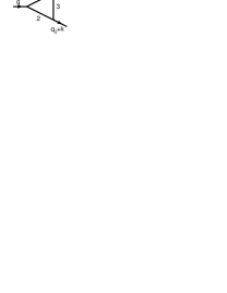
Figure 3: Oneloop subgraph $C(k)$

The purpose of this paper is to calculate typical two-loop IR-divergent vertex diagrams by two independent methods. One of them is based on general formulae for asymptotic expansions of Feynman integrals in momenta and masses [5, 6] (see [7] for a brief review) and subsequent use of conformal mapping and summation by Padé approximations [1, 2]. The general simple formulae have been proven [6] at least for the Feynman integrals off the mass shell. However it is quite natural to expect that the same off-shell formulae hold as well for the pure large mass limit when there are no large momenta, as it has been confirmed in ref. [2]. This conjecture is likely to hold even for Feynman integrals which possess IR and collinear divergences from the very beginning. To check the validity of this conjecture we shall calculate IR-divergent diagrams 7 and 8 shown in Fig. 1 (the labelling is according to [2], Fig. 3) by use of the large mass expansion and compare results in a wide range of external momenta with results based on numerical integration.

The project is motivated by the demand to provide the necessary integrals for the process $Z\rightarrow b\bar{b}$. The before-mentioned divergences appear in the limit $m_{b}\to 0$, which is a natural limit to take since $m_{b}$ is small compared to the other scales in this process. The case of a finite $m_{b}$ mass can in principle also be handled by both methods, see e.g. Ref. [9] for the momentum expansion method applied to a finite diagram ($Case~{}5$, $m_{5}=m_{6}=M$, all others zero, see Fig. 1). In this case, however, one obtains less precise results because of the low thresholds, which are eliminated in the present approach due to the factorization of logarithms. For the numerical method the case $m_{b}\neq 0$ presents no difficulty.

The numerical methods, as introduced in [3, 4, 10, 11] are in the present paper extended to the case of IR and collinear divergences. We will explain this extension below. The two methods used in this paper are of complementary nature. While for the method based on the large mass expansion the equal mass case is simpler than the case of different masses, the situation is reversed if we apply the two-fold integral representation. The presence of poles of the type $\lim_{m_{1}\to m_{2}}1/(m_{1}-m_{2})$ in the integral representations results in numerical instabilities which have to be handled with due care. Corresponding poles in the first method can be avoided from the very beginning by calculating the Taylor coefficients analytically in terms of rational numbers and $\zeta(2)$ for the equal mass case. In the case of nonequal masses the Taylor coefficients contain such poles of high order (see below), which cancel in the $\lim_{m_{1}\to m_{2}}$. Numerically a close approach is possible due to the use of a multiple precision package [12].

The idea of the numerical approach is now well documented in the literature. We will thus restrict ourselves to describe the necessary changes demanded by the presence of IR and collinear divergences. These changes are simple: one merely has to find subtraction terms to absorb the divergences, which are sufficiently easy to allow for a direct evaluation. So there was no new conceptual challenge present in the numerical method, but solely a technical hurdle to be overcome.

The paper is organized as follows. First, we discuss the method based on the large mass expansion for $Cases~{}7$ and $8$, considering the equal as well as different masses in $Case~{}7$. We then discuss the relevant subtraction terms for the numerical method. Once they are understood, all the previous cases can be easily obtained. We summarize the results in a set of tables, and compare accuracies and CPU times for both methods. We finally conclude that the agreement of data obtained by the two independent methods confirms the usefulness of both.

Figure 1: On-shell infrared divergent planar diagrams with zero thresholds (solid lines massive, dashed lines massless).

2 $Case~{}7$

2.1 Equal masses

Let $F_{\Gamma}(p_{1},p_{2},M;\varepsilon)$ be the Feynman integral corresponding to $Case~{}7$, with $m_{3}=m_{4}=m_{5}=0,\;m_{1}=m_{2}=m_{6}=M,\;p_{1}^{2}=p_{2}^{2}=0,q=p_{1}-p_{2}$. We imply that the factor $1/(k^{2}-m^{2}+i0)$ corresponds to a line, $1/(2\pi)^{d}$ is not included. For convenience we divide our Feynman integrals by $i\pi^{d/2}\Gamma(1+\varepsilon)\mu^{-2\varepsilon}$ per loop, where $d=4-2\varepsilon$ is the space-time dimension and $\mu$ the scale parameter of dimensional regularization [13] (although we shall not usually write down $\mu$ explicitly).

Although the diagram has IR poles, up to $1/\varepsilon^{2}$, let us apply the general formula for the large mass expansion [5, 6] (as it was applied for similar IR-finite planar diagrams in Ref. [2]). There are contributions from two subgraphs in this formula: the graph $\Gamma\equiv\gamma_{1}$ itself and $\gamma_{2}=\{126\}$ (we denote subgraphs by collections of their lines). The first, “naive”, contribution is the formal Taylor expansion of the initial diagram in external momenta. It reduces to two-loop vacuum graphs with numerators, two massive and one massless line. This term possesses IR divergences that were not present from the very beginning.

The second contribution is nothing but the Taylor expansion of the heavy triangle (with $p_{1}+k_{2},p_{2}+k_{2}$ as external momenta, $k_{2}$ being the loop momentum of the light triangle) inserted into the light triangle. Now, this heavy triangle is a scalar function of three variables: $(p_{1}+k_{2})^{2},(p_{2}+k_{2})^{2}$ and $q^{2}$. When performing its Taylor expansion, the factor $(p_{1}+k_{2})^{2}$ leads to a cancellation of one of the lines in the light triangle. This produces a one-loop massless diagram with its external momentum on the lightcone. It is zero within dimensional regularization. Thus we come to the conclusion that only terms without such factors survive and one can put $k_{2}$ to zero in the expansion of the heavy triangle. So, the term under consideration happens to be just a product of two factors: the light triangle with zero masses and the Taylor expansion of the heavy triangle with $p_{1},p_{2},p_{1}-p_{2}$ as external momenta. The light triangle is equal to

$$-\frac{1}{\varepsilon^{2}}\frac{\Gamma(1-\varepsilon)^{2}}{\Gamma(1-2\varepsilon)}\frac{1}{(-q^{2}-i0)^{1+\varepsilon}}.$$ (1)

(We shall later on omit $-i0$ in $-q^{2}-i0$, for brevity.)

The Taylor expansion of the heavy triangle is also calculated explicitly:

$$-\frac{1}{(M^{2})^{1+\varepsilon}}\frac{1}{\Gamma(1+\varepsilon)}\sum_{n=0}^{\infty}\frac{\Gamma(n+1+\varepsilon)}{2(n+1)(2n+1)!!}(q^{2}/2M^{2})^{n}.$$ (2)

The second term does not involve UV divergences, in contrast to the large mass expansions considered in Ref. [2]. In large mass expansions (as well as large momentum expansions off the mass shell) induced IR divergences are usually cancelled by induced UV divergences. Here we have an example of a new cancellation: the induced IR divergences are cancelled by collinear divergences that are present in the second term. To a large extent this happens when we put to zero the above mentioned one-loop massless diagram on the lightcone where the UV divergences are cancelled by the collinear divergences.

Thus the contribution of the second subgraph takes the form (with the normalization described above)

$$-\frac{1}{q^{2}}\frac{1}{M^{2}}(-q^{2}/\mu^{2})^{-\varepsilon}(M^{2}/\mu^{2})^{-\varepsilon}\frac{1}{\varepsilon^{2}}\frac{\Gamma(1-\varepsilon)^{2}}{\Gamma(1+\varepsilon)\Gamma(1-2\varepsilon)}$$

$$\times\sum_{n=0}^{\infty}\frac{\Gamma(n+1+\varepsilon)}{2(n+1)(2n+1)!!}(q^{2}/2M^{2})^{n}.$$ (3)

If an initial quantity is finite the cancellation of poles serves as a good check of the asymptotic expansion. In our case, it is reasonable to check that the poles in the sum of the terms in our expansion are the same as in the initial diagram. To see that the poles in $\varepsilon$ in the sum of the two contributions are the same as in the initial Feynman integral let us apply the following expression for the pole part in $\varepsilon$ of the product of three propagators, namely, $1/k^{2},1/(k^{2}-2p_{1}k)$ and $1/(k^{2}-2p_{2}k)$ considered as a distribution in $k$:

$$i\frac{\pi^{2-\varepsilon}}{(-q^{2})^{1+\varepsilon}}\left\{\left(-\frac{1}{\varepsilon^{2}}+\gamma_{\rm E}\frac{1}{\varepsilon}\right)\delta^{(d)}(k)+\frac{1}{\varepsilon}\int_{0}^{1}\frac{\mbox{d}z}{z}[\delta(k-zp_{1})+\delta(k-zp_{2})-2\delta(k)]\right\}.$$ (4)

It is easy to observe that the term with $\delta^{(d)}(k)$ exactly corresponds to the pole part of the second contribution. Thus, the term with the integral over $z$ should give the pole part of the naive contribution. Let us therefore calculate the integral over $z$ of the rest of the diagram (which is nothing but a one-loop triangle diagram with the external momenta $(1-z)p_{1},p_{2}-zp_{1}$, plus a similar contribution, with $p_{2}$ instead of $p_{1}$). Representing the result in the form of a Taylor expansion in the external momenta we conclude that the pole part in $\varepsilon$ of the naive part is equal to

$$\frac{1}{M^{4}}\frac{1}{\varepsilon}\sum_{n=0}^{\infty}\frac{s_{n+1}(n+1)!}{2(n+2)(2n+3)!!}(q^{2}/2M^{2})^{n},$$ (5)

where $s_{n}=S_{1}(n)$ and we introduce

$$S_{k}(n)=\sum_{j=1}^{n}\frac{1}{j^{k}}.$$ (6)

This property has served as a check in our calculation.

The double pole in $\varepsilon$ comes only from $\gamma_{2}$. Using (3) we obtain the following explicit expression for the coefficient at $1/\varepsilon^{2}$:

$$-\frac{2}{(q^{2})^{2}}\arcsin^{2}\sqrt{q^{2}/4M^{2}}\,.$$ (7)

The naive part is calculated as described in [2], see also [14]. The two-loop bubble integrals with equal masses and one zero mass are again of the type as used in [2], i.e. expressible in terms of $\Gamma$-functions as a result of which the Taylor coefficients of the naive part are essentially rational numbers (apart from a $\zeta(2)$ as for the second contribution. These Taylor coefficients have been calculated with FORM [15] and the Padé approximants in turn by means of REDUCE [16], which allows an easy change to floating point numbers of arbitrary precision. Adding up the finite parts, the results are presented in Table 1 with the following normalization. In addition to $-\pi^{d}\Gamma(1+\varepsilon)^{2}\mu^{-4\varepsilon}$, we extract the factor $\frac{\Gamma(1-\varepsilon)^{2}}{\Gamma(1-2\varepsilon)}\frac{1}{\mu^{4}}$, and we choose $\mu=M$.

2.2 Two different masses

Proceeding as before in $Case~{}7$ with two different masses, $m_{3}=m_{4}=m_{5}=0,\;m_{1}=m_{2}=M_{1},\;m_{6}=M_{2}$, we come to the following result for the contribution of the second subgraph:

$$\frac{1}{(-q^{2})^{1+\varepsilon}}\frac{1}{(M_{2}^{2})^{\varepsilon}}\frac{1}{\varepsilon^{2}}\frac{\Gamma(1-\varepsilon)^{2}}{\Gamma(1+\varepsilon)\Gamma(1-2\varepsilon)}\sum_{n=0}^{\infty}n!\left\{\Gamma(-n-1+\varepsilon)\frac{(M_{2}^{2})^{n+1}}{(M_{2}^{2}-M_{1}^{2})^{2n+2}}\right.$$

$$\left.+\left(\frac{M_{2}^{2}}{M_{1}^{2}}\right)^{\varepsilon}\;\sum_{i=0}^{2n+1}\frac{(-1)^{i}\Gamma(n-i+\varepsilon)}{(2n-i+1)!}\frac{(M_{1}^{2})^{i-n}}{(M_{2}^{2}-M_{1}^{2})^{1+i}}\right\}(q^{2})^{n}.$$ (8)

Calculation of the pole and finite parts allows for the representation

$$\frac{r_{2}}{\varepsilon^{2}}+\frac{r_{1}-r_{2}L}{\varepsilon}+r_{0}-r_{1}L+\frac{1}{2}r_{2}L^{2}\,,$$ (9)

where $L=\ln M_{2}^{2}+\ln(-q^{2})$ and

$$r_{0}=\frac{1}{2M_{1}^{2}q^{2}}\sum_{n=0}^{\infty}n!(q^{2}/M_{1}^{2})^{n}$$

$$\times\left\{\sum_{i=0}^{n-1}\frac{(n-i-1)!}{z^{i+1}(2n-i+1)!}\left(\ln^{2}(1-z)-2\zeta(2)+2\ln(1-z)s_{n-i-1}+s^{2}_{n-i-1}+t_{n-i-1}\right)\right.$$

$$+\sum_{i=n}^{2n+1}\frac{(-1)^{i-n}}{3z^{i+1}(i-n)!(2n-i+1)!}\left(3\ln^{2}(1-z)s_{i-n}\right.+3\ln(1-z)(s^{2}_{i-n}-t_{i-n})$$

$$+3s_{n+1}t_{n+1}+\ln^{3}(1-z)+s^{3}_{i-n}-s^{3}_{n+1}\left.\left.+u_{i-n}-u_{n+1}-3s_{i-n}t_{i-n}\right)\right\},$$

$$r_{1}=\frac{1}{M_{1}^{2}q^{2}}\sum_{n=0}^{\infty}n!(q^{2}/M_{1}^{2})^{n}\left\{\sum_{i=0}^{n-1}\frac{(n-i-1)!}{z^{i+1}(2n-i+1)!}(\ln(1-z)+s_{n-i-1})\right.$$

$$-\sum_{i=n}^{2n+1}\frac{(-1)^{i-n}}{2z^{i+1}(i-n)!(2n-i+1)!}\left(-\ln^{2}(1-z)-2\ln(1-z)s_{i-n}\right.$$

$$\left.\left.-s^{2}_{i-n}+t_{i-n}+s^{2}_{n+1}-t_{n+1}\right)\right\},$$

$$r_{2}=\frac{1}{M_{1}^{2}q^{2}}\sum_{n=0}^{\infty}n!(q^{2}/M_{1}^{2})^{n}$$

$$\times\left\{\sum_{i=0}^{n-1}\frac{(n-i-1)!}{z^{i+1}(2n-i+1)!}+\sum_{i=n}^{2n+1}\frac{(-1)^{i-n}\left(\ln(1-z)+s_{i-n}-s_{n+1}\right)}{z^{i+1}(i-n)!(2n-i+1)!}\right\},$$

where $t_{n}=\zeta(2)-S_{2}(n)$ and $u_{n}=-2\zeta(3)+S_{3}(n)$, $S_{k}(n)$ given by Eq. (6) and $z=1-M_{2}^{2}/M_{1}^{2}$. The importance of presenting the above formulae lies in their easy numerical evaluation. If instead we would use the expanded form, 30 coefficients could not even be compiled anymore simultaneously.

We also calculate (in the same way as in the case with equal masses) a quantity, the pole part of which is equal to the pole part of the naive contribution:

$$\frac{1}{q^{2}}\frac{1}{\varepsilon}\sum_{n=1}^{\infty}n!\sum_{j=1}^{n}\frac{1}{j}$$

$$\times\left\{(-1)^{j}\sum_{i=0}^{j}{2n-j+i+1\choose 2n-j+1}\frac{\Gamma(j-i-n-1+\varepsilon)}{(j-i)!}\frac{(M_{2}^{2})^{n+i-j+1-\varepsilon}}{(M_{2}^{2}-M_{1}^{2})^{2n-j+i+2}}\right.$$

$$\left.+\sum_{i=0}^{2n-j+1}{j+i\choose j}\frac{(-1)^{i}\Gamma(n-j-i+\varepsilon)}{(2n-j-i+1)!}\frac{(M_{1}^{2})^{i+j-n-\varepsilon}}{(M_{2}^{2}-M_{1}^{2})^{j+i+1}}\right\}(q^{2})^{n}.$$ (10)

Explicitly, this gives

$$\frac{1}{\varepsilon}\frac{2}{M_{1}^{2}q^{2}}\sum_{n=1}^{\infty}n!(q^{2}/M_{1}^{2})^{n}$$

$$\times\sum_{j=1}^{n}\frac{(-1)^{j}}{j}\left\{(-1)^{n}\sum_{i=0}^{j}{2n-j+i+1\choose 2n-j+1}\frac{s_{n-j+i+1}(1-z)^{n-j+i+1}}{(j-i)!(n-j+i+1)!z^{2n-j+i+2}}\right.$$

$$\left.+\sum_{i=0}^{n-j-1}{j+i\choose j}\frac{(n-j-i-1)!}{(2n-j-i+1)!z^{j+i+1}}+\sum_{i=0}^{n+1}(-1)^{i}{n+i\choose j}\frac{\ln(1-z)+s_{i}}{i!(n+1-i)!z^{n+i+1}}\right\}\,.$$ (11)

Furthermore this representation of the pole part has been used as a check of the naive part.

Finally there remains to calculate the finite contribution of the naive part. Again we proceed as in [2] and [14]. The difficulty arising now is a complication in the bubble integrals with two different masses and one zero mass (e.g., $m_{3}=0$):

$$V_{B}(\alpha,\beta,\gamma,m_{1},m_{2},m_{3})=\frac{(-1)^{(\alpha+\beta+\gamma)}}{(i{\pi}^{\frac{d}{2}})^{2}}\int\frac{d^{d}k_{1}d^{d}k_{2}}{(k_{1}^{2}-m_{1}^{2})^{\alpha}(k_{2}^{2}-m_{2}^{2})^{\beta}((k_{1}-k_{2})^{2}-m_{3}^{2})^{\gamma}},$$ (12)

Apart from $\Gamma$-functions these contain now the hypergeometric function ${~{}}_{2}F_{1}(a,b,c;z)$ with the argument $z=1-\frac{m_{1}^{2}}{m_{2}^{2}}\leq 1$ [17] ($z=0$ and ${~{}}_{2}F_{1}=1$ in the equal mass case!). Therefore it does not seem to be advisable anymore to use FORM for the evaluation of the Taylor coefficients since too complicated expressions would arise. Instead we extended a program developed for arbitrary nonzero masses [9] based on the multiple precision FORTRAN by D.H. Bailey [12]. In this framework the occurrence of a zero mass, i.e. the additional IR divergences cause the following complication: while for arbitrary nonzero masses only the bubble integrals

$$V_{B}(1,1,n,m_{1},m_{2},m_{3})=F(1,1,n,m_{1},m_{2},m_{3})+\frac{1}{\varepsilon}~{}\frac{1}{(n-1)(n-2)}\frac{1}{(m^{2}_{3})^{\left(n-2\right)}},~{}n>2,$$ (13)

(F($\cdots$) being the finite part) are divergent like $\frac{1}{\varepsilon}$ (apart from $V_{B}(1,1,1)$ and $V_{B}(1,1,2)$ which have also $\frac{1}{{\varepsilon}^{2}}$ -terms), in the present case all the needed bubble integrals $V_{B}(1,m,n)$ with $m\geq 1$ and $n\geq 3$ have a $\frac{1}{\varepsilon}$-term, which is to be calculated by means of the hypergeometric function ${~{}}_{2}F_{1}(a,b,c;z)$ with integer indices $a,b,c$ ($d=4$) and $c=a+b+1$. This ${~{}}_{2}F_{1}$ can be expressed in terms of $ln(1-z)$ and powers of $z$ and $1-z$.

Knowing the divergent parts of the bubble integrals explicitly, the recursion for their finite part can be performed and the complete contribution to the finite part of the diagram can be calculated.

Finally two further remarks are in order. The first concerns the evaluation of the second subgraph. As one observes from the Taylor series of $r_{0},r_{1}$ and $r_{2}$ in (9), these contain high powers of $\frac{1}{z}$. In the equal mass case ($z=0$), the expansion of the $ln(1-z)$ to high powers cancels all inverse powers of $z$ and the finite coefficients as described in Sect. 2.1 are obtained. Numerically, however, due to the use of the multiple precision program of Bailey [12] for mass ratios close to 1 (e.g. $z\sim 10^{-3}$) still stable results in close agreement with the equal mass case can be obtained.

The second remark concerns adding up of the various contributions. There are two possibilities: one can sum the different series ( for $r_{0},r_{1}$ etc. ) by means of Padé ’s, multiply the various results with the corresponding powers of $L$ (see e.g. (9)) and sum — or one can add up on the level of the coefficients, multiplying the Taylor coefficients with the powers of $L$, and then apply Padé ’s. We used the latter procedure since the coefficients are known to high precision (of the order of 50 decimals). The summed series were of course by far not that precise and if cancellations occur, one looses more precision than necessary. That in this manner correct results are obtained is demonstrated by comparing the results with those by the numerical method (see tables).

While in the present paper adding different Taylor series with kinematical factors is performed for the calculation of one diagram only, the same procedure will also work when adding scalar amplitudes from various Feynman diagrams - and may indeed work in an optimal way.

For the pole parts we do not show tables since they are either given explicitly in terms of known functions or arbitrarily many coefficients can be obtained easily and thus arbitrarily high precision. The results for the finite part are presented in Table 2. We use the same normalization as in the case with the equal masses and choose $\mu=M_{1}$.

3 $Case~{}8$

Let here $F_{\Gamma}(p_{1},p_{2},M;\varepsilon)$ be the Feynman integral corresponding to $Case~{}8$, with $m_{i}=0,\;i=1,\ldots,5,\;m_{6}=M$. Now, in its large mass expansion, we have contributions from four subgraphs: $\gamma_{1}\equiv\Gamma,\gamma_{2}=\{3456\},\gamma_{3}=\{126\}$, and $\gamma_{4}=\{6\}$. In the last two contributions, the factor (1) is again naturally factorized. Straightforward calculation leads to the following result for the sum of them:

$$-\frac{1}{(M^{2})^{1+\varepsilon}}\frac{1}{(-q^{2})^{1+\varepsilon}}\frac{1}{\varepsilon^{3}}\frac{\Gamma(1-\varepsilon)^{3}}{\Gamma(1-2\varepsilon)}$$

$$\times\left\{\sum_{n=0}^{\infty}\frac{n!}{\Gamma(n+2-\varepsilon)}(-q^{2}/M^{2})^{n}-(-q^{2}/M^{2})^{-\varepsilon}\sum_{n=0}^{\infty}\frac{\Gamma(n+1-\varepsilon)}{\Gamma(n+2-2\varepsilon)}(-q^{2}/M^{2})^{n}\right\}.$$ (14)

The calculation of the contribution of $\gamma_{2}$ is similar to the corresponding calculations for Cases 1 and 5 in ref. [2], with the following result:

$$\frac{1}{(M^{2})^{2+\varepsilon}}\frac{1}{(-q^{2})^{\varepsilon}}\frac{1}{\varepsilon}\sum_{n=0}^{\infty}c^{(2)}_{n}(\varepsilon)(q^{2}/M^{2})^{n},$$ (15)

where

$$c^{(2)}_{n}(\varepsilon)=\sum_{{i_{1},i_{2},n_{3}\geq 0,\;i_{1}+i_{2}+n_{3}\;\mbox{\scriptsize even}}\atop{i_{1}+i_{2}+n_{3}\leq 2n}}\sum_{j_{3}\geq 0}^{(n_{3},-2)}(-1)^{(i_{1}+i_{2}+n_{3})/2}\;\frac{(n-(i_{1}+i_{2}-n_{3})/2)!}{(n-(i_{1}+i_{2}+n_{3})/2)!}$$

$$\times\frac{i_{1}!i_{2}!\theta(i_{1}+i_{2}-j_{3})\theta(i_{1}-i_{2}+j_{3})\theta(-i_{1}+i_{2}+j_{3})}{((n_{3}-j_{3})/2)!((i_{1}+i_{2}-j_{3})/2)!((i_{1}-i_{2}+j_{3})/2)!((-i_{1}+i_{2}+j_{3})/2)!}$$

$$\times\frac{\Gamma(1-\varepsilon)\Gamma((i_{1}+i_{2}-j_{3})/2+1-\varepsilon)}{\Gamma(1+\varepsilon)\Gamma((i_{1}+i_{2}-j_{3})/2+2-2\varepsilon)}$$

$$\times C(1+i_{2},3+n+(i_{1}-i_{2}+n_{3})/2;(i_{1}+i_{2}+n_{3})/2),$$ (16)

and

$$C(r_{1},r_{2};s)=\frac{\Gamma(r_{1}+r_{2}-s-\frac{d}{2})\Gamma(s-r_{2}+\frac{d}{2})}{\Gamma(r_{1})\Gamma(s+\frac{d}{2})}.$$ (17)

Note that this expression is obtained from the corresponding contribution of $Case~{}5$ in [2] by the change

$$C(2+i_{1}+i_{2},2+n-(i_{1}+i_{2}-n_{3})/2;(i_{1}+i_{2}+n_{3})/2)$$

$$\to C(1+i_{2},3+n+(i_{1}-i_{2}+n_{3})/2;(i_{1}+i_{2}+n_{3})/2).$$

To see that the poles in $\varepsilon$ in the sum of all the four contributions are the same as in the initial Feynman integral let us once again apply eq. (4). Now we observe that the term with $\delta^{(d)}(k)$ corresponds to the pole part of the sum of the contributions from $\gamma_{3}$ and $\gamma_{4}$ given by (14). Thus, the term with the integral over $z$ should give the pole part of the sum of contributions from $\gamma_{1}$ and $\gamma_{2}$. So, we perform integration over $z$ of the one-loop triangle diagram with one non-zero and two zero masses. Furthermore we apply general formulae for the large mass expansion to this very triangle and eventually conclude that the pole part in $\varepsilon$ of the sum of the contributions from $\gamma_{1}$ and $\gamma_{2}$ should be equal to the pole part of the following quantity:

$$\frac{1}{q^{2}}\frac{1}{(M^{2})^{1+\varepsilon}}\frac{2}{\varepsilon\Gamma(1+\varepsilon)}\sum_{n=1}^{\infty}n!\left(\sum_{j=1}^{n}\frac{C(j+1,2n-j+2;n)}{j}\right)(q^{2}/M^{2})^{n}$$

$$+2\frac{1}{(-q^{2})^{1+\varepsilon}}\frac{1}{M^{2}}\frac{\Gamma(1-\varepsilon)}{\varepsilon^{2}}\sum_{n=1}^{\infty}\frac{s_{n}\Gamma(n+1-\varepsilon)}{\Gamma(n+2-2\varepsilon)}(-q^{2}/M^{2})^{n}.$$ (18)

Note that double poles in (18) cancel so that there must be as well a cancellation of double poles in the sum of the contributions of $\gamma_{1}$ and $\gamma_{2}$. Again this has been checked and also that the single pole part agrees with the one obtained by direct calculation of the sum of $\gamma_{1}$ and $\gamma_{2}$.

For $Case~{}8$, the double pole in $\varepsilon$ originates only from the sum of the contributions of $\gamma_{3}$ and $\gamma_{4}$. From (14) we have the following formula for its coefficient:

$$\frac{1}{(q^{2})^{2}}\left\{\ln(-q^{2}/M^{2})\ln(1+q^{2}/M^{2})+\mbox{Li}_{2}(-q^{2}/M^{2})\right\}\,.$$ (19)

Concerning the finite part, the situation is similar as in Sect. 2.1, $Case~{}7$, with equal masses. The bubble integrals are of the same type as in $Case~{}5$ [2] and the calculation of the Taylor coefficients have been done with FORM and the Padé ’s with REDUCE. Again we present no data for the divergent parts since arbitrary precision can easily be obtained from the expansion. The results for the finite part are presented in Table 3 where the same normalization as in $Case~{}7$ is used.

4 The Numerical Method

The two-fold integral representation derived in [18, 3, 10] cannot be naively applied to cases infected by genuine IR or collinear divergences. Nevertheless, all these divergences can be handled by appropriate subtraction terms. One observes a few new characteristics in such cases:

• the divergences are most easily absorbed using lightcone coordinates for internal momenta in the parallel space,

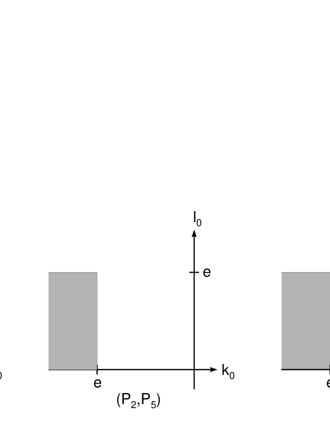
Figure 5: Contributions from term 3

• some of the remaining domains of integration are unbounded, cf. Fig.(5).

We will comment on these features in the next three subsections.

4.1 Preparations

The graph we have to calculate is

$$I = \mu^{2d-12}\int d^{d}kd^{d}l\frac{1}{P_{1}P_{2}P_{3}P_{4}P_{5}P_{6}}$$ (20)

$$= \mu^{2d-12}\int d^{d}k\frac{1}{P_{4}P_{5}P_{6}}C(k)\,,$$

where $C(k)$ denotes the inner one-loop triangle graph with external momenta shifted by $k$ (Fig. 3).

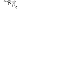
Figure 2: Propagator numbering, external and loop momenta

For our calculation, we choose the rest frame of the decaying particle and the outgoing particles moving along the $x$ axis. This is the natural reference frame for parallel-/orthogonal space splitting. Together with the condition that both outgoing momenta are on the lightcone, the external momenta can be expressed through a single parameter $e$ (cf. Fig. 2):

$$q=q_{1}+q_{2} = (2e,0,\vec{0})$$

$$q_{1} = (e,e,\vec{0})$$

$$q_{2} = (e,-e,\vec{0})$$ (21)

As usual we parameterize the loop momenta $l$ and $k$ as follows:

$$l^{\mu}=(l_{0},l_{1},\vec{l}_{\perp})\quad\mbox{and}\quad k^{\mu}=(k_{0},k_{1},\vec{k}_{\perp})\,,$$ (22)

further we define

$$s=l_{\perp}^{2}\quad\mbox{and}\quad t=k_{\perp}^{2}\,.$$ (23)

In contrast to [3, 10] we apply a more symmetric substitution to linearize the propagators in $l_{0}$, $l_{1}$, $k_{0}$ and $k_{1}$ (the Jacobian gives a factor 2 for each loop momentum):

$$l_{0} \to l_{0}+l_{1}$$

$$l_{1} \to l_{1}-l_{0}$$

$$k_{0} \to k_{0}+k_{1}$$

$$k_{1} \to k_{1}-k_{0}\,,$$ (24)

which is equivalent to expressing the propagators in lightcone variables from the beginning. After this substitution the propagators become

$$P_{1} = 4l_{0}(l_{1}+e)-s-m_{1}^{2}+i0$$

$$P_{2} = 4l_{1}(l_{0}-e)-s-m_{2}^{2}+i0$$

$$P_{3} = 4(l_{0}+k_{0})(l_{1}+k_{1})-s-t-\sqrt{s}\sqrt{t}z-m_{3}^{2}+i0$$

$$P_{4} = 4k_{0}(k_{1}-e)-t-m_{4}^{2}+i0$$

$$P_{5} = 4k_{1}(k_{0}+e)-t-m_{5}^{2}+i0$$

$$P_{6} = 4k_{0}k_{1}-t-m_{6}^{2}+i0$$ (25)

Since we are interested in the collinear divergent case, we now set $m_{4}$ and $m_{5}$ equal to 0, $m_{6}$ should be kept small for the finite contribution as a regulator. The limit will be made later analytically. The calculation is valid for arbitrary masses $m_{1}$, $m_{2}$ and $m_{3}$, except for the trivial case $m_{1}=m_{2}=m_{3}=0$.

In this representation the collinear divergence along the lines $k_{0}=0$ and $k_{1}=0$ for $t=0$ is obvious. To cure it, we adopt the following subtraction scheme for $C(k)=C(k_{0},k_{1},t)$:

$$\begin{array}[]{rclr}C(k_{0},k_{1},t)&=&\hphantom{+}C(k_{0},k_{1},t)-C(k_{0},0,0)-C(0,k_{1},0)+C(0,0,0)&(I)\\ &&+C(k_{0},0,0)-C(0,0,0)&(II)\\ &&+C(0,k_{1},0)-C(0,0,0)&(III)\\ &&+C(0,0,0)\,.&(IV)\end{array}$$ (26)

Contribution (I) will be finite and can be calculated in $d=4$ dimensions, since we subtracted out the collinear divergences and added again the twice subtracted infrared divergence at $k\equiv 0$. Contributions (II) and (III) contain the collinear divergence which starts at $1/\varepsilon$, and (IV) is the overall infrared divergence with a $1/\varepsilon^{2}$ pole. Therefore these have to be calculated in $d=4-2\varepsilon$ dimensions.

4.2 Divergent parts

Contribution (IV) is easy: it is simply a product of two one-loop diagrams, where the $k$ loop is completely massless:

$$I_{\rm IV}=-i\pi^{d/2}\frac{\Gamma^{2}\left(\frac{d-4}{2}\right)\Gamma\left(\frac{6-d}{2}\right)}{\Gamma\left(d-3\right)}(-q^{2}-i0)^{\frac{d-6}{2}}C(0,0,0)\,.$$ (27)

The expansion of the $\Gamma$ functions starts with $1/\varepsilon^{2}$, so $C(0,0,0)$ has to be calculated up to ${\cal O}(\varepsilon^{2})$. The last order is done numerically.

Contribution (II) is more complicated, since the $l$ and $k$ integrations do not decouple. However, the integrand is independent of $z$, the angle between $\vec{l}_{\perp}$ and $\vec{k}_{\perp}$, so there is no function with a cut in the complex $k_{1}$ plane. We have

$$I_{\rm II} = \frac{\pi^{\frac{d-2}{2}}}{2\Gamma\left(\frac{d-2}{2}\right)}\int\limits_{-\infty}^{+\infty}dk_{0}\big{(}C(k_{0},0,0)-C(0,0,0)\big{)}\int\limits_{0}^{\infty}t^{\frac{d-4}{2}}dt\int\limits_{-\infty}^{+\infty}dk_{1}\frac{1}{P_{4}P_{5}P_{6}}\,,$$ (28)

and perform the $k_{1}$ integration with Cauchy’s theorem. We close the contour in the lower half plane, and there is only a contribution from $P_{5}$ in the finite interval $0<k_{0}<e$, outside this interval all poles are on the same side of the real axis.

The integration over $t$ is of the form

$$\int\limits_{0}^{\infty}dt\frac{t^{\frac{d-6}{2}}}{t+4k_{0}(k_{0}+e)}=(4k_{0}(k_{0}+e))^{\frac{d-6}{2}}\Gamma\left(\frac{d-4}{2}\right)\Gamma\left(\frac{6-d}{2}\right)\,,$$ (29)

so after a substitution $k_{0}=-ze$ the result is

$$I_{\rm II} = -i\pi^{d/2}\frac{\Gamma\left(\frac{d-4}{2}\right)\Gamma\left(\frac{d-6}{2}\right)}{\Gamma\left(\frac{d-2}{2}\right)}(-q^{2}-i0)^{\frac{d-6}{2}}$$ (30)

$$\int\limits_{0}^{1}dz\frac{1}{z}\left[z(1-z)\right]^{\frac{d-4}{2}}\left(C(ze,0,0)-C(0,0,0)\right)\,.$$

The expansion of the $\Gamma$ functions starts at $1/\varepsilon$, so the integral over $z$, which will be done numerically, has to be evaluated up to ${\cal O}(\varepsilon)$.

Contribution (III) can be handled analogously by performing the $k_{0}$ integration with Cauchy’s theorem and gives

$$I_{\rm III} = -i\pi^{d/2}\frac{\Gamma\left(\frac{d-4}{2}\right)\Gamma\left(\frac{d-6}{2}\right)}{\Gamma\left(\frac{d-2}{2}\right)}(-q^{2}-i0)^{\frac{d-6}{2}}$$ (31)

$$\int\limits_{0}^{1}dz\frac{1}{z}\left[z(1-z)\right]^{\frac{d-4}{2}}\left(C(0,ze,0)-C(0,0,0)\right)\,.$$

For the symmetric case $m_{1}=m_{2}$, $I_{\rm III}$ is equal to $I_{\rm II}$.

4.3 The finite part

The most difficult is the finite part from contribution (I). In principle, the calculation is the same as in [3, 10], but care has to be taken due to the divergent behavior of the individual parts of this contribution. The integration over $z$, the angle between $\vec{l}_{\perp}$ and $\vec{k}_{\perp}$, is elementary for each for the four terms. In fact, only the first term with the full $C(k_{0},k_{1},t)$ dependence depends also on $z$, and therefore gives a result with a cut in the complex $l_{1}$ and $k_{1}$ plane.

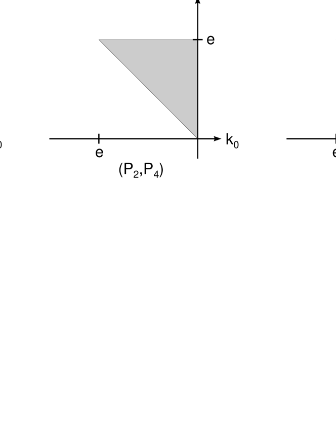
Figure 4: Contributions from terms 1 and 2

The $l_{1}$ and $k_{1}$ integrations are done with the aid of the residue theorem. Each term is still convergent on its own, so the contours can be closed independently. For the $C(k_{0},k_{1},t)$ term we have to take into account the cut which is in the upper half plane if $l_{0}+k_{0}<0$ and in the lower half plane if $l_{0}+k_{0}>0$. By checking the half plane where the propagators have their poles, we find three contributing triangles in the $(l_{0},k_{0})$ plane from the pairs $(P_{1},P_{5})$, $(P_{2},P_{4})$ and $(P_{2},P_{6})$, depicted in Fig. 4.

For the second term, $C(k_{0},0,0)$, we can close the contours arbitrarily. If we choose to close them in the same way as above (this is equivalent to avoiding poles from $P_{3}$, the propagator that depends on both loop momenta) we find the same triangles from the same propagators as above.

With $C(0,k_{1},0)$ we find something new in our parallel/orthogonal space technique: regardless how we close the contours, we end up with an unbounded area in the $(l_{0},k_{0})$ plane. If we continue with the strategy of avoiding poles from $P_{3}$, we have to close the $l_{1}$ contour in the upper half plane if $l_{0}>0$ and in the lower half plane if $l_{0}<0$, furthermore we close the $k_{1}$ contour always in the upper half plane. This gives us the three areas shown in Fig. 5 from $(P_{2},P_{4})$, $(P_{2},P_{5})$ and $(P_{2},P_{6})$ respectively.

For last term $C(0,0,0)$, which factorizes in $l$ and $k$ we can close so that in the $l_{1}$ integration only $P_{2}$ contributes, and in the $k_{1}$ integration only $P_{5}$. This results in a square (Fig. 6).

Next we will do the $t$ and later the $s$ integration analytically. Since we left $m_{6}$ finite, after partial fractioning the integrals are of the form

$$\int\limits_{0}^{\infty}ds\int\limits_{0}^{\infty}dt\frac{1}{s+s_{0}-i0}\frac{1}{t+t_{0}-i0}\frac{1}{\sqrt[c]{(at+b+i0+cs)^{2}-4st}}$$ for term 1

$$\int\limits_{0}^{\infty}ds\int\limits_{0}^{\infty}dt\frac{1}{s+s_{0}-i0}\frac{1}{t+t_{0}-i0}\frac{1}{at+b+i0+cs}$$ for term 2 & 3

$$\int\limits_{0}^{\infty}ds\int\limits_{0}^{\infty}dt\frac{1}{s+s_{0}-i0}\frac{1}{s+s_{0}^{\prime}-i0}\frac{1}{t+t_{0}-i0}\frac{1}{t+t_{0}^{\prime}-i0}$$ for term 4. (32)

Several of these integrals become divergent as $m_{6}\to 0$, whenever the corresponding $t_{0}$ is proportional to $m_{6}$. Consequently, the leading term is proportional to $\log(m_{6})$. However, as can be verified, pairs of the above integrals remain finite in the limit $m_{6}\to 0$. The pairs depend on the position in the $(l_{0},k_{0})$ plane (area A, B or C, Fig. 7).

5 Numerical Results

Tables 1–3 summarize the results. Generally, there are two sets of results for the momentum expansion method, namely two $[n/n]$ Padé approximants involving $2n+1$ Taylor coefficients, which document that the results are stable and converge. It is the second column which should be compared with the numerical data.

Let us now discuss the three cases separately. $Case~{}7$ with equal masses, Table 1, was the most challenging for the numerical method. Below the threshold, we could achieve sufficient numerical accuracy. Above the threshold, the numerical method could only achieve an accuracy of $\sim 1$%. Fortunately, for the equal mass case, M. Spira could kindly provide data which were used for comparison with the momentum expansion method to high accuracy. The lack of accuracy in the numerical method in this case is due to the degenerate cut structure which is present in the equal mass case. As a result, we are confronted with two large contributions which almost cancel.

In $Case~{}7$ with different masses, Table 2, we chose the masses $m_{1}=m_{2}=80GeV(\sim M_{W})$ and $m_{6}=180GeV(\sim M_{t})$ and $\mu=m_{1}$. If we wish to calculate the process $Z\rightarrow b\bar{b}$ the kinematics of interest is $q^{2}/m_{1}^{2}\sim 1.3$, i.e. far below the threshold at $q^{2}/m_{1}^{2}=4$. In such a situation the momentum expansion method always seems to be superior to any other approach (to achieve 10 decimals precision with a few coefficients only is no problem). Nevertheless, also for low $q^{2}$ the numerical method yields high precision as well which will be sufficient for all practical purposes. Indeed the agreement is quite impressive.

For higher $q^{2}$ the momentum expansion method naturally gets less precise, in particular near the thresholds: here $q^{2}=4m_{1}^{2}$ and $q^{2}=(m_{1}+m_{6})^{2}$, i.e. $q^{2}/m_{1}^{2}\sim 10.6$. Between the thresholds and above, both methods again show surprisingly good agreement.

The situation is indeed quite different for $Case~{}8$. While for the case of interest in $Z\rightarrow b\bar{b}$, i.e. $q^{2}/m_{1}^{2}=1$ both approaches yield approximately the same precision, the momentum expansion method looses quickly for the higher $q^{2}$, i.e. many more Taylor coefficients would be needed.

Quite generally speaking the results of the momentum expansion method obtained so far seem to indicate that the more heavy masses in a diagram occur, the better the convergence of the Padé approximants. This is at least qualitatively plausible since we start from a large mass expansion. It is also numerically verified comparing $Case~{}7$ and 8.

In any case, splitting off systematically zero-mass thresholds yields more precise results for the momentum expansion method than keeping small but non-vanishing masses resulting in low thresholds. This has been discussed in [9] for $Case~{}5$ (i.e. $m_{5}=m_{6}=M$ and all others 0, see Tables 3 and 4 of that Ref.). For the numerical method to handle such cases is much easier. In fact, one could rely on the original integral representations [3, 10] without the modifications considered here and achieve much better numerical results for all cases.

Concerning the CPU-time, comparison of the methods is difficult. In the momentum expansion method the real job is to calculate the Taylor coefficients. Once they are known, for any $q^{2}$ (in the complex plane) the calculation of the diagram under consideration is a matter of seconds. Thus, providing Taylor coefficients for the diagrams is something which practically settles the calculation of the diagrams under consideration once for all in a wide range of $q^{2}$. This is in particular true if only one nonzero mass is involved since in this case the Taylor coefficients are just rational numbers plus some well known irrationals like $\zeta(2)$, $\zeta(3)$ etc. The methods to calculate Taylor coefficients are at present still a matter of intense investigation (see e.g. also [19]) and the hope is that we will soon have more efficient methods for their calculation and higher coefficients than used here can be obtained in the future.

For the numerical method, we can give a rough estimate by comparison with the results of [3]. Due to the extra subtraction terms, the CPU time needed here is about an order of magnitude larger than in the IR- and collinear convergent cases studied in [3].

6 Conclusion

Two different methods to calculate scalar two-loop vertex diagrams with infrared and collinear divergences have been investigated and interesting techniques for their calculation have been developed. An important case with different masses has been solved, which is a step forward to a realistic calculation of the two-loop decay $Z\rightarrow b\bar{b}$. The results show that both methods deliver consistent results. This confirms the expectation that the two techniques developed are applicable in the demanding cases considered here.

Acknowledgement

We are grateful to M. Spira for providing us with numerical data for the $Case~{}7$ with equal masses. J.F. is grateful to O. Veretin and T. Kotikov for helpful discussions. K.S. would like to thank Ben Grinstein and the UCSD physics department for their hospitality.

Table 1. The finite part for $Case~{}7$ with equal masses.

Table 1. The finite part for $Case~{}7$ with equal masses.

	$q^{2}/M^{2}$		[10/10]				[14/14]				numerical results
			Re		Im		Re		Im		Re		Im
1	.0	2	.764761286	$-$0	.1635351018	2	.764761286	$-$0	.1635351018	2	.76477	$-$0	.16353
2	.0	1	.619771096	0	.4534319337	1	.619771096	0	.4534319337	1	.61977	0	.45344
3	.0	1	.477131552	0	.5068403285	1	.477131552	0	.5068403285	1	.47713	0	.50684
3	.9	3	.0354569	0	.28920132	3	.035456900	0	.2892013177	3	.03546	0	.28920
3	.99	5	.1725	0	.0143	5	.17259	0	.014233	5	.17253	0	.014236
4	.01	6	.188	2	.748	6	.187	2	.749	6	.18778	2	.74948
4	.1	3	.27648	3	.92262	3	.27645	3	.92263	3	.27646	3	.92263
5	.0	$-$0	.438728	2	.54547	$-$0	.438728258	2	.545472409	$-$0	.438728	2	.54548
6	.0	$-$0	.89277747	1	.49214654	$-$0	.8927774793	1	.492146568	$-$0	.892777	1	.49215
7	.0	$-$0	.90571711	0	.92720655	$-$0	.9057171008	0	.9272065484	$-$0	.905717	0	.927207
8	.0	$-$0	.828158487	0	.59820497	$-$0	.8281584836	0	.5982049870	$-$0	.828159	0	.598205
10	.0	$-$0	.65092293	0	.26109287	$-$0	.6509229304	0	.2610928562	$-$0	.650923	0	.261093
40	.0	$-$0	.07133439	$-$0	.0467805	$-$0	.0713343755	$-$0	.0467805683	$-$0	.0713345	$-$0	.0467805
100	.0	$-$0	.0126312	$-$0	.0182863	$-$0	.012631500	$-$0	.018286325		N/A		N/A
400	.0	$-$0	.000556	$-$0	.002743	$-$0	.00055586	$-$0	.00274078	$-$0	.000555895	$-$0	.00274078

Table 2. The finite part for $Case~{}7$ with different masses.

Table 2. The finite part for $Case~{}7$ with different masses.

	$q^{2}/m_{1}^{2}$		[12/12]				[15/15]				numerical results
			Re		Im		Re		Im		Re		Im
1	.0	1	.255976034	0	.4303855857	1	.255976034	0	.4303855857	1	.255974	0	.430385
2	.0	0	.6127661221	0	.4991658334	0	.6127661221	0	.4991658334	0	.61277	0	.499164
3	.0	0	.4346988621	0	.4502907526	0	.4346988621	0	.4502907526	0	.43470	0	.450292
3	.9	0	.4583945	0	.34378450	0	.458394486	0	.343784488	0	.4584	0	.34379
3	.99	0	.4926	0	.2501	0	.49254	0	.25004761	0	.4925	0	.25003
4	.01	0	.637	0	.190	0	.6359	0	.1902	0	.63598	0	.18994
4	.1	0	.73506	0	.43258	0	.73504	0	.43260	0	.73526	0	.43271
5	.0	0	.32211	0	.855621	0	.322110	0	.855622	0	.32219	0	.85569
6	.0	0	.00752	0	.802352	0	.0075200	0	.8023528	0	.00756	0	.80237
7	.0	$-$0	.16178	0	.682114	$-$0	.161777	0	.682110	$-$0	.16176	0	.68214
8	.0	$-$0	.25256	0	.56468	$-$0	.252547	0	.564693	$-$0	.25255	0	.56469
10	.0	$-$0	.3259	0	.3799	$-$0	.3256	0	.37987	$-$0	.32559	0	.37975
40	.0	$-$0	.06956	$-$0	.02984	$-$0	.0695667	$-$0	.029828	$-$0	.06956	$-$0	.02983
100	.0	$-$0	.01350	$-$0	.01529	$-$0	.013493	$-$0	.015279	$-$0	.01349	$-$0	.01528
400	.0	$-$0	.00072	$-$0	.00253	$-$0	.00071	$-$0	.002537	$-$0	.00071	$-$0	.00254

Table 3. The finite part for $Case~{}8$.

Table 3. The finite part for $Case~{}8$.

	$q^{2}/m_{6}^{2}$		[12/12]				[15/15]				numerical results
			Re		Im		Re		Im		Re		Im
0	.5	81	.17501719	12	.06458720	81	.17501719	12	.06458720	81	.1750	12	.0644
1	.0	17	.766	19	.97799834	17	.7659	19	.97799834	17	.7658	19	.9779
2	.0	$-$0	.605	7	.376	$-$0	.6047	7	.3759	$-$0	.604	7	.376
3	.0	$-$1	.753	3	.182	$-$1	.7543	3	.1815	$-$1	.754	3	.182
4	.0	$-$1	.596	1	.606	$-$1	.595	1	.603	$-$1	.595	1	.604
5	.0	$-$1	.33	0	.881	$-$1	.327	0	.880	$-$1	.326	0	.880
6	.0	$-$1	.10	0	.50	$-$1	.096	0	.503	$-$1	.095	0	.503
7	.0	$-$0	.92	0	.28	$-$0	.914	0	.289	$-$0	.913	0	.288
8	.0	$-$0	.77	0	.15	$-$0	.773	0	.159	$-$0	.771	0	.159
10	.0	$-$ 0	.56	0	.01	$-$ 0	.572	0	.023	$-$ 0	.570	0	.025

Figure 6: Contribution from term 4

Figure 7: Integration regions in the $(l_{0},k_{0})$ plane

References

- [1] J. Fleischer and O.V. Tarasov, Z. Phys. C 64 (1994) 413.
- [2] J. Fleischer, V.A. Smirnov and O.V. Tarasov , Z. Phys. C74 (1997) 379.
- [3] A. Czarnecki, U. Kilian, D. Kreimer, Nucl. Phys. B433, 259 (1995).
- [4] A. Frink, B.A. Kniehl, D. Kreimer, K. Riesselmann, Phys. Rev. D54 (1996) 4548.
- [5] S.G. Gorishny, preprints JINR E2–86–176, E2–86–177 (Dubna 1986); Nucl. Phys. B319 (1989) 633; K.G. Chetyrkin, Teor. Mat. Fiz. 75 (1988) 26; 76 (1988) 207; K.G. Chetyrkin, preprint MPI-PAE/PTh 13/91 (Munich, 1991); S.G. Gorishny and S.A. Larin, Nucl. Phys. B 283 (1987) 452; S.A. Larin, T. van Ritbergen and J.A.M. Vermaseren, Nucl. Phys. B 438 (1995) 278.
- [6] V.A. Smirnov, Commun. Math. Phys. 134 (1990) 109; V.A. Smirnov, Renormalization and asymptotic expansions (Birkhäuser, Basel, 1991).
- [7] V.A. Smirnov, Mod. Phys. Lett. A 10 (1995) 1485.
- [8] V.A. Smirnov, Phys. Lett. B394 (1997) 205; A. Czarnecki and V.A. Smirnov, Phys. Lett. B394 (1997) 211; V.A. Smirnov, hep-ph/9703357.
- [9] J. Fleischer and O.V. Tarasov, Proceedings of the 1966 Zeuthen Workshop on Elementary Particle Theory: QCD and QED in higher Orders; Rheinsberg Germany 21-26 April 1966. Nucl. Phys. B (Proc. Suppl.) 51C (1966); J. Blümlein, F. Jegerlehner and T. Riemann editors.
- [10] A. Frink, U. Kilian, D. Kreimer, Nucl.Phys.B488 (1997) 426.
- [11] L. Brücher, J. Franzkowski, A. Frink, D. Kreimer, ‘An Introduction to XLOOPS , MZ-TH/96-39A-D, hep-ph/9611378, 4 talks, all to appear in Nucl.Instr.Meth.Phys.Res.A, Presented at 5th International Workshop on New Computing Techniques in Physics Research (AIHENP96), Lausanne, Switzerland, 2-6 Sep 1996.
- [12] D.H. Bailey, ACM Transactions on Mathematical Software, 19 (1993) 288.
- [13] G. ’t Hooft and M. Veltman, Nucl. Phys. B44 (1972) 189; C.G. Bollini and J.J. Giambiagi, Nuovo Cim. 12B (1972) 20.
- [14] J. Fleischer and O.V. Tarasov, in proceedings of the ZiF conference on Computer Algebra in Science and Engineering, Bielefeld, 28-31 August 1994, World Scientific 1995, J. Fleischer, J. Grabmeier, F.W. Hehl and W. Küchlin editors.
- [15] J.A.M. Vermaseren, Symbolic manipulation with FORM (Amsterdam, Computer Algebra Nederland, 1991).
- [16] A.C. Hearn, REDUCE User’s manual, version 3.5, RAND publication CP78 (Rev.10/93).
- [17] F.A. Berends, A.I. Davydychev, V.A. Smirnov and J.B. Tausk, Nucl. Phys. B439 (1995) 536.
- [18] D. Kreimer, Phys. Lett. B292, 341, (1992).
- [19] O.V. Tarasov, Nucl.Phys. B 480 (1996) 397.