PRA-HEP 97/06


On the role of power expansions in quantum field theory

abstract

Methods of summation of power series relevant to applications in quantum theory are reviewed, with particular attention to expansions in powers of the coupling constant and in inverse powers of an energy variable. Alternatives to the Borel summation method are considered and their relevance to different physical situations is discussed. Emphasis is placed on quantum chromodynamics. Applications of the renormalon language to perturbation expansions (resummation of bubble chains) in various QCD processes are reported and the importance of observing the full renormalization-group invariance in predicting observables is emphasized. News in applications of the Borel-plane formalism to phenomenology are conveyed. The properties of the operator-product expansion along different rays in the complex plane are examined and the problem is studied how the remainder after subtraction of the first $n$ terms depends on the distance from euclidean region. Estimates of the remainder are obtained and their strong dependence on the nature of the discontinuity along the cut is shown. Relevance of this subject to calculations of various QCD effects is discussed.

PACS numbers: 11.55.Hx, 11.55.Fv

April 1997

1 Introduction

1.1 Perturbation series

A typical situation in physics is want of exact solutions. To find a good approximation of a problem, we have mostly first to simplify it by neglecting a number of effects, thereby facilitating its solution but, simultaneously, endangering its physical relevance. It is a general experience that exact equations can mostly be solved only approximately.

Perturbation theory (PT) is based on the idea of expressing the solution $f(g)$ to a problem (equation) in the form of the power series

$$\sum_{n=0}^{\infty}f_{n}g^{n},$$ (1)

where $g$, the perturbative parameter, is considered to be a small numerical quantity describing, possibly, a physically important effect.

The first question to ask is how $f(g)$ is related to the series (1). To approach it, we have to see (i) what is the precise meaning of (1) and, (ii), in what sense the series (1) is assigned to $f(g)$, the searched solution to the problem. For this to discuss, we have to consider complex values of $g$.

Simplest is the situation when $f(g)$ is holomorphic inside a circle of radius $\rho>0$ centred at the origin; then (1) is the Taylor expansion of $f(g)$ and determines $f(g)$ uniquely, $f(g)$ being equal to (1) for all $|g|<\rho$. The $f_{n}$ are given by the derivatives of $f(g)$ at the origin.

If, however, $\rho=0$, the equality

$$f(g)=\sum_{n=0}^{\infty}f_{n}g^{n}\,\,,$$ (2)

being valid only for $g=0$, is not relevant for applications. On the other hand, if we assume, instead of (2), an asymptotic relation between $f(g)$ and (1),

$$f(g)\sim\sum_{n=0}^{\infty}f_{n}g^{n}$$ (3)

for $g\rightarrow 0$, there is always an $f(g)$ satisfying (3) for any set $\{f_{n}\}$ [1]. Further, in contrast to (2), the relation (3) does not determine the function $f(g)$ uniquely, even when all the $f_{n}$ are explicitly given and the set of rays approaching the point $g=0$ is specified. Even then a whole class of functions $f(g)$ is defined by (3). The situation changes if additional restrictions are imposed on the remainder $f(g)-\sum_{n=0}^{N}f_{n}g^{n}$; then there may be only one function satisfying the requirements, and we can call it the sum of the series.

Such additional restrictions as well as the assumptions (2), (3) themselves should be motivated physically. Equation (2) is related to the question of convergence:

• /1/ (Convergence): Is the series convergent, in the sense that the limit of

  $$f_{(N)}(g)=\sum_{n=0}^{N}f_{n}g^{n}$$ (4)

  for $N\rightarrow\infty$, with $g$ fixed, exists? For what values of $g$ is this the case?

  The asymptoticity property (3), on the other hand, is a statement on smoothness:

• /2/ (Smoothness): Is the expression

  $$|f(g)-\sum_{n=0}^{N}f_{n}g^{n}|$$ (5)

  bounded, in what domain of $(N,g)$ (with $g$ complex and $N$ a nonnegative integer) and what is the bounding function?

  Finally, there is the question of uniqueness:

• /3/ (Uniqueness): Can the sequence $\{f_{n}\}$, $n=1,2$,…, uniquely determine the expanded function $f(g)$ and under what conditions?

Perturbation theory yields, at least in principle, explicitly all the coefficients $f_{n}$ of the expansion (1). The knowledge of the large-order behaviour of the $f_{n},n=1,2$,…, tells us whether the series (1) is convergent or not, but what we really need is to answer the question /3/, i.e., that of a unique determination of $f(g)$. If $f(g)$ is holomorphic at the origin, (1) is convergent and $f(g)$ is uniquely determined from the coefficients $f_{n}$ by means of (2). There was a universal belief till the early 1950’s that a sound physical theory should not use a divergent perturbation expansion or a function singular at the origin.

In 1952, F.J. Dyson [3] argued that in QED there is a singularity at the origin of the complex coupling-constant plane. (The conjecture that such a singularity makes the series divergent was questioned later, see [4] and references therein.)

A wide class of divergent series can be given precise meaning by means of Borel summation, provided that certain additional conditions are imposed on $f(g)$. This method has found fruitful applications in quantum field theory, where its use goes back to the 1950’s. In 1951, for example, J. Schwinger [5] obtained a compact expression for the term in the Lagrangian corresponding to the QED vacuum polarization by an external constant magnetic field $H$. Then V. Ogievetsky [6] used the (divergent) perturbative expansion of this term to show that its Borel sum coincides with Schwinger’s result. Indeed, the coefficients of its perturbative expansion in powers of $e^{2}$ behave as $(2n-3)!(-H^{2}/(\pi^{2}m^{4}))^{n}$ at large $n$, where $e$ and $m$ is the charge and the mass of the electron respectively. Ogievetsky found the Borel sum in the form

$$\int_{0}^{\infty}{\rm e}^{-m^{2}t}a(t,e){\rm d}t$$ (6)

with

$$a(t,e)=-\frac{1}{8\pi^{2}t^{3}}[etH\cot(etH)-1-(etH)^{2}/3],$$ (7)

which coincides with the compact expression obtained by Schwinger [5]. This important result shows that a divergent perturbative expansion does not signal an inconsistency in a theory; it also shows that there are special - but realistic - cases of Borel summability in QED, although general considerations indicate Borel non-summability (see [7, 9, 10], and Table 1 and a discussion in section 2 of the present paper).

Gradually, the Borel summation techniques became widely adopted in quantum theory. It even became common to judge theories according to whether their perturbation expansions are Borel summable or not; in this sense, the formal criterion of Borel summability became successor to the criterion of convergence. Being rather technical assumptions, however, neither convergence nor Borel summability can serve as criteria of consistency of a theory. One might find it more natural to set another criterion of consistency: that the transition from the perturbed to the unperturbed state should be continuous and smooth in the coupling parameter. But even this is not necessary: Nature is not obliged to be smooth in our parameters. It is a special step to assume that the transition from the world with interaction, $g>0$, to that without it ($g=0$) is smooth. This is why the relation (3) has nontrivial physical implications.

Disregarding special field theories with interactions being interpreted as discontinuous perturbations in the sense that the theory does not return to the unperturbed theory as the interaction coupling vanishes, the fact is that asymptotic expansions in powers of $g$ have been universally adopted in quantum theory; perturbation theory does imply the assumption of a smooth transition from the state with interaction to that without it. What we then really need is to answer the question /3/ of uniqueness, which is independent both of convergence and of Borel summability. If the answer to /3/ is yes, i.e., if the $f_{n}$ determine $f(g)$ uniquely, the theory could be considered as selfsufficient, no matter whether the conditions of Borel summability are satisfied or not. If the answer is no, the theory has to be supplemented with some additional input.

In the majority of situations in physics, $f(g)$ has a singularity at the origin; note that smoothness at a point does not exclude a singularity at this point. Then the perturbation expansion is not a Taylor series and, if considered as an asymptotic expansion, it needs a supplement for uniqueness to be reached. Needless to say, this supplement should be of physical nature, while no formal argument (e.g., that the method yields a finite value of a divergent series) can fill the gap where physics is missing.

1.2 Large-order behaviour

The problem of the high-order behaviour of the perturbation-expansion coefficients in field theory calculations has aroused new interest in the last decade. Particular attention has been paid to power corrections to QCD predictions for hard scattering processes. One can point out two reasons for this growing interest:

• The theoretical problem of how physical observables can be reconstructed from their (often divergent) power expansions.

• The pragmatic need to assess the usefulness of performing the extensive evaluations of multi-loop Feynman diagrams in QCD. Much effort has been devoted to the computation of higher-order QCD perturbative corrections; in some cases third-order approximations are known, and we now seem to be at the border of what can be carried out analytically or numerically in high-order perturbative calculations. So, why next order? If the series is divergent, the next order may represent no improvement with respect to the lower-order result. On the contrary, at a certain order it will lead to deterioration.

The question of the possible divergence of asymptotic perturbation expansions, which goes back to the original argument of Dyson [3], still defies definite and clear answer. Notice in this connection that a series that is asymptotic to a function singular at the origin need not be divergent. Indeed, for any series (1) convergent within a circle $|g|<\rho$ there are functions $f(g)$ which are singular at $g=0$ and have (1) as asymptotic series. The traditional wisdom that the divergence of perturbation expansions is directly related to the discontinuities of Green’s functions is not generally true. If the series is asymptotic, the knowledge of the large-order behaviour of perturbation-theory coefficients is insufficient for the determination of the function expanded and one needs much more detailed information in the vicinity of the point of expansion in order to establish the relation between the expansion and the function expanded.

In fact most of the information on the analytic properties of relevant Green’s functions near $g=0$ [9, 11] may actually be invisible in perturbation expansions themselves. Moreover, the summability of a perturbation expansion is not the same as the possibility of recovering from such series the corresponding full physical quantity. As the summability of QCD perturbation expansions is determined by the large-order behaviour of their coefficients, we primarily need to know which kind of information is necessary to explicitly obtain the sum of the series.

If a theory provides, in addition to the values of the expansion coefficients ${f_{n}}$, enough supplementary information, a power series can be summed to a finite number, which is not arbitrary but reflects the additional piece of information used. One has to give it such a form that it could be used to reduce (or even remove) the ambiguity connected with the asymptoticity of the expansion. The task of a summation method then is not to assign arbitrarily an ad hoc value (whose only merit might just be that it is finite) to your infinite or ambiguous series, nor to fill the gap in physics (which your theory possibly possesses) with some mathematical cement, but to offer you a service: to translate your physical idea (or that of the theory you work with) into a mathematical condition to reduce the ambiguity of the formal power series.

As a typical example of this procedure the role of general principles in the $S$-matrix theory can be mentioned. The $S$-matrix techniques were built from mathematically formulated, but physical principles: analyticity as a mathematical formulation of microscopic causality, unitarity as probability conservation, crossing symmetry as a general property of Feynman diagrams, and the position and character of the cut in the complex energy plane as a description of the properties of the particle spectrum. A simultaneous use of the analyticity properties and of the concepts of field theory was carried out in the QCD Sum Rules program [12], which met with tremendous phenomenological success. Note that the foundation of this approach rests on the non-trivial fact [13, 14] that the principles of $S$-matrix theory are rigorously true in QCD: it follows [14] that for gauge theories, if confinement is imposed, the analytic properties of physical amplitudes are the same as those obtained from an effective theory involving only the composite (physical) fields.

It should be considered as very fortunate that, simultaneously, analyticity plays a crucial role also as a mathematical condition reducing the ambiguity of asymptotic series. In Section 2 of the present paper, we discuss in detail the interplay between large-order behaviour of a series (as listed in Table 1) and the analyticity properties of the function expanded; it turns out that a balance between these two concepts is needed for a unique determination of $f(z)$ from (3), in the sense that if more analyticity of $f(z)$ is available, one can afford a more violent behaviour of the $a_{n}$, and vice versa.

In Section 3 we focus on some practical aspects of the operator-product expansion, in particular on the problem of how the remainder after subtraction of the first $n$ terms from the function expanded depends on the distance from euclidean region, provided that an estimate on the remainder in euclidean region is known. Sections 4 and 5 are devoted to singularities in the Borel plane and applications of the Borel plane formalism to phenomenology. We discuss the progress in understanding the role of the singularities in the Borel plane for nonperturbative effects, in studying hadrons containing heavy quarks, then the different methods of calculation of the coupling constant $\alpha_{s}$ from existing experimental data, the role of operator product expansion in practical calculations and the progress in the resummation of bubble chains. Section 6 is devoted to problems related to renormalization ambiguities and their impact on phenomenology. Section 7 contains concluding remarks. Some parts of the present paper represent an extended and amended version of ref. [15].

Below we give a survey of the large-order behaviour of perturbative series in different theories. Bender and Wu [16] examined perturbation theory for one-dimensional quantum mechanics with a polynomial potential and they obtained the large-order behaviour of the perturbation coefficients. Lipatov [18] obtained the same results for massless renormalizable scalar field theories.

Brézin, Le Guillou and Zinn-Justin [19], applying independently the same method to anharmonic oscillations in quantum mechanics, were able to rederive and generalize the results obtained by Bender and Wu.

In QED, after the pioneering work of Dyson [3], a number of papers appeared discussing the analyticity properties of the Green functions (some of them are cited in refs. [4] and [20]). The growth like $n!$ (where $n$ is the order of approximation) has two sources:

1. The number of diagrams grows like $n!$, each diagram giving a contribution of the order of 1.

2. There are types of diagrams for which the amplitude itself grows like $n!$ [21].

A survey of the large-order behaviour of expansion coefficients in some typical theories and models is given in the Table 1. As subtle cancellations among higher-order graphs may occur, the expressions in the third column of Table 1 may sometimes give an upper bound rather than the actual high-order behaviour of the coefficients.

Table 1 is intended for first information and should not be used for systematic analyses because some important conditions or restrictions could not be mentioned. A brief explanation of its use is given below. Notation is not consistent, being mostly taken from the papers quoted; the reader is referred to them for explanation. References in the table as well as in the text are often made not to the original papers but rather to more recent papers or reviews, in which the subject is explained in modern context. As a result, a number of valuable papers are not quoted. I apologize for this. For details I refer to the papers cited and references therein, and to the anthology by Le Guillou and Zinn-Justin [20], which contains a list of references up to  1990.

Theory	Notation and references	High-order behaviour
1 Disp. relation	${\rm Im}f(z)\sim z^{-b}{\rm e}^{-a/z}$	$f_{n}\sim(-a)^{n}\Gamma(n+b)$
2 Anharmonic	$E_{m}(g)=\sum_{n=0}^{\infty}E_{m,n}g^{n}$	$E_{m,n}\sim(-3/4)^{n}n!$
2 oscillator	[16]
3 Anharmonic	$I(g)\sim\int_{-\infty}^{\infty}{\rm e}^{(-x^{2}/2-gx^{4}/4)}{\rm d}x$	$I_{n}\sim(-1)^{n}4^{-n}(n-1)!$
3 oscillator,    $\phi^{4}$	[20]
4 $\phi^{4}$ in 2 and	[25]	Analyticity for complex $g$,
4 3 dimensions	[26]	Borel summability proved
5 Instantons,	$m\geq 6$, [18]	$C_{n}(m)\sim(-\tilde{g})^{n}{\rm e}^{n(1-m/2)}n^{(m+D)/2}$
5 $D=2m/(m-2)$	$m=4$, [18]	$C_{n}(4)\sim 2.75n^{4}(n/(16\pi^{2}e))^{n}$
6 Field theories	$Z_{n}=\sum_{k=0}^{\infty}Z_{n}^{(k)}(-e^{2}/(4\pi))^{k}$	$Z_{n}^{(k)}\sim k!k^{b_{n}}A^{-k}c_{n}[1+O(1/k)]$
without fermions	[19],[27] - [30]
7 Field theories	[8]	$A_{n}\sim\Gamma(n(d-2)/d)R^{n}n^{-\alpha}\cos(2\pi n/d)A$
7 with fermions	[31]	$f_{n}\sim(-1)^{n}S^{n/2}\Gamma(n/2)D$
8 Yukawa theories	[8]	$Z_{n}\sim n^{-\alpha}A^{-n}{\rm cos}(2\pi n/d)\Gamma(n(d-2)/d)$
Yuk $d=2$	[32]	$d_{n}\sim A^{-n}(\ln\,n)^{n}$
9 QED	[31, 33]	$f_{n}\sim(-1)^{n}\Gamma((n+\nu)/2)a^{n+\nu}$
	[44] (1st IR renormalon)	$d_{n}\sim{\rm const}(-\beta_{0}/2)^{n}\Gamma(n+1-2\beta_{1}/\beta_{0}^{2})$
	[45]	$r_{n}\sim{\rm const}\,\beta_{0}^{n}n!\,n^{2+\beta_{1}/\beta^{2}_{0}+\gamma_{2}}$
10 QCD in 2 dim.	[46]	$(g^{2}N_{c}/2)^{2k}(-1)^{k-1}(2k)!$
11 QCD	[11, 34, 47, 48]	$f_{n}\sim a^{n}n^{\gamma}n!$
	see [44, 45] for discussion	$d_{n}\sim{\rm const}(-\beta_{0}/2)^{n}\Gamma(n+1-2\beta_{1}/\beta_{0}^{2})$
12 Bosonic strings	$h$ is # of handles,   [22]	$\sim h!$

Table 1: High-order behaviour of perturbation expansion coefficients
(see also explanations in the text)

A few words on the explanation of the symbols used in the table. In the item 1, $f(z)$ is a real function analytic in the complex $z$ plane cut along $[-\infty,0]$ and equal to $\int_{-\infty}^{0}{\rm d}z^{\prime}{\rm Im}f(z^{\prime})/(z^{\prime}-z)$. In item 2, the $E_{m}(g)$ are, for $g>0$, the eigenvalues of the Hamiltonian $H=-\frac{1}{2}({\rm d/d}q)^{2}+\frac{1}{2}q^{2}+\frac{1}{4}gq^{4}$.

Eckmann, Magnen and Sénéor [25] consider the two-dimensional Euclidean boson field theories and give bounds on truncated Schwinger functions. They also prove that the domain of analyticity and of the bounds obtained can be extended to an angle $>\pi$ bisected by the positive real semiaxis, and prove the Borel summability of the power series of the Schwinger functions. In the case of the Euclidean $\phi^{4}$ theory in 3 dimensions, Magnen and Sénéor [26] prove the stability of the free energy for complex values of the coupling constant and obtain, in analogy with the two-dimensional case, Borel summability of the perturbation series.

In the instanton row (item 5), the $C_{n}(m)$ are the coefficients of the expansion of the Gell-Mann–Low function, with $n$ being the perturbative order and $m$ being related to the dimension $D$ by $D=2m/(m-2)$. Further, both $C_{n}(m)$ and $C_{n}(4)$ contain an $n$-independent (but $m$-dependent) factor.

The item 6 is related to scalar electrodynamics in four dimensions, with the action

$$S(\phi,A_{\mu})=\int{\rm d}^{4}x\left[\frac{1}{4}F_{\mu\nu}^{2}+\frac{1}{2}|D_{\mu}\phi|^{2}+\frac{1}{2}m^{2}|\phi|^{2}+\lambda|\phi|^{4}/4!\right].$$ (8)

The $Z_{n}$ are one-particle irreducible Euclidean Green’s functions, with $c_{n},b_{n}$ and $A$ being constants and $A$ being equal to 12 approximately.

For field theories with fermions (item 7), $A(g)=\sum_{n}A_{n}g^{2n}$ is the Green function of the scalar field $\sigma$ with the coupling term $g\sigma\bar{\Psi}\Psi$ for a Yukawa interaction in $d>2$ dimensions [8]; $R,\alpha$ and $A$ are computable constants. In ref. [31], the $f_{n}$ denote the main contribution to the QED perturbation theory asymptotics, where $S$ is equal to $3^{-3/2}4\pi^{3}$.

The $d_{n}$ in the item 9 describe (see [44]) the asymptotic behaviour of perturbation series due to the first infrared renormalon in QED. (In QCD, item 11, the result agrees with that obtained by relating infrared renormalons to nonperturbative corrections.) The $d_{n}$ are the coefficients in the perturbative expansion of the function $Q^{2}{\rm d}/({\rm d}Q^{2})\,\,P(Q^{2})$ in powers of the coupling parameter $\alpha(Q)$,

$$\sum_{n=-1}d_{n}\alpha(Q)^{n+1}.$$ (9)

In QED, $\alpha P$ is equal to $\Pi$, the photon vacuum polarization, and $d_{-1}=-\beta_{0}$, $\beta_{0}$ is the first coefficient in the expansion of the beta function, which is defined as $\mu^{2}{\rm d}/{\rm d}\mu^{2}\,\,\alpha(\mu)=\beta(\mu)=\sum_{n=0}\beta_{n}\alpha(\mu)^{n+2}$. In QCD, $P=\Pi$ is the electromagnetic current-current correlation function. The large-order behaviour in QCD is $d_{n}\sim{\rm const}(-\beta_{0}/2)^{n}\Gamma(n+1-2\beta_{1}/\beta_{0}^{2})(1+{\rm O}(n))$. Beneke and Zakharov [44] show that in QED (with massless fermions), the coefficients $d_{n}$ have the same IR behaviour with $\beta_{n}$ taking their QED values. The UV renormalons are also present and produce the fixed-sign divergence of the perturbative series. They have been analyzed by Beneke and Smirnov [45], who study classes of diagrams with an arbitrary number of chains, and derive explicit formulae for leading and subleading divergence. To organize the diagrams in classes, the expansion parameter $1/N_{f}$ is used, where $N_{f}$ is the number of fermion species; as a consequence, diagrams suppressed in the $1/N_{f}$ expansion are not suppressed for large $n$ and, consequently, no finite order in the $1/N_{f}$ expansion provides the correct behaviour in $n$ in the full theory. Table 1 shows the large-order behaviour of the vacuum polarization, $r_{n}$ being the coefficient of i$\alpha^{n+1}$ in the perturbative expansion and $\gamma_{2}=99/(8N_{f}^{2})$ . The authors discuss extension of the formalism to non-abelian gauge theories and expect a similar result.

For QCD in 2 dimensions (with $N_{c}$ tending to infinity), Zhitnitsky [46] argues that the factorial growth $(g^{2}N_{c}/2)^{2k}(2k)!(-1)^{k-1}$ of the large-order perturbative coefficients is related to instantons, thus being of non-perturbative nature. Important in this theory is dimensionality of the coupling constant.

Gross and Periwal [22] (see item 12) proved that the $h$-loop bosonic partition function (cut off in the infrared region) is bounded below and the perturbative expansion for the bosonic string diverges as $\sum_{h=0}^{\infty}g^{2h}\,h!$. The series is not Borel summable, all its terms being positive.

A look at the third column of Table 1 shows that most of the theories listed are characterized by an $n!$ large-order behaviour. This does not mean that all of them can be cured by the same resummation method: large-order behaviour is just one of aspects which determine the summation procedure. To each power series with coefficients listed in the 3rd column of Table 1, there is a whole class of functions $f(z)$ having the same asymptotic expansion. To specify the asymptotic expansion, one has to establish the angle (ray(s)) along which $z$ approaches the origin; further, to pick out one function $f(z)$ of this class, one has to add some additional information, according to the theory in question.

As was already mentioned, these additional conditions are often formulated in terms of analyticity properties of the function expanded.

In the next section, let us discuss the character of the additional conditions.

2 Asymptotic series. Summation methods

If you are in doubt,

examine the asymptotics

How to deal with divergent series and under which conditions a power series can uniquely determine the expanded function are questions of fundamental importance in quantum theory. Power expansions are badly needed in physics, but additional input is required to ensure that they have precise meaning. These additional conditions should reflect some physical features of the system.

We shall change the notation in this section, introducing the symbol $z$ for the coupling parameter denoted previously by $g$.

A formal series (1) is called asymptotic to $f(z)$ on the set ${\cal S}$ if the sequence $R_{N}(z)$,

$$R_{N+1}(z)=f(z)-\sum_{0}^{N}f_{n}z^{n}$$ (10)

satisfies the condition

$$R_{N+1}(z)=o(z^{N})$$ (11)

for all non-negative integers $N$ and all $z\,\in\,{\cal S}$, where ${\cal S}$ is a subset of the complex plane having the origin as an accumulation point.

The analogous notion of a series for which (10) and (11) are satisfied only for a limited number of $N$, $N=0,1,2,...,N_{0}$, has also interesting applications.

It is important that ${\cal S}$ is generally a subset of the neighbourhood of the origin. As an example to illustrate non-uniqueness, consider (3) for $z$ approaching zero within the angle $|\arg z|<\beta$ with $\beta\leq\pi/2$, i.e., in the right-hand half of the complex plane. To a function $f(z)$ satisfying (3), one can add a term of the form $A\exp(-1/z^{a})$ with $A$ real and $0<a<\pi/(2\beta)$ without violating (11) within ${\cal S}$.

A summation method states conditions under which an asymptotic series can determine $f(z)$ uniquely, and yields the explicit formula for $f(z)$.

2.1 Uniqueness by Borel summation

The series

$$\sum_{n=0}^{\infty}a_{n}z^{n}$$ (12)

is called Borel summable if

1) its Borel transform $B(t)$,

$$B(t)=\sum_{n=0}^{\infty}a_{n}t^{n}/n!,$$ (13)

converges inside some circle, $\mid t\mid<\delta\,,\,\,\delta>0$;

2) $B(t)$ has the analytic continuation to an infinite strip of non-vanishing width bisected by the positive real semi-axis ${\rm Re}\,\,t\geq 0$, and

3) the integral

$$g(z)=\frac{1}{z}\int_{0}^{\infty}{\rm e}^{-t/z}B(t){\rm d}t\,,$$ (14)

called the Borel sum, converges for some $z\neq 0$.

One can see the motivation of this summation method on a simple example. Consider a generic quantity $D$, calculated in perturbation theory with the coupling $z$,

$$D(z)=\sum_{n=0}^{\infty}d_{n}z^{n}\,.$$ (15)

This can be rewritten as

$$D(z)=\sum_{n=0}^{\infty}d_{n}z^{n}(1/n!)\int_{0}^{\infty}{\rm d}t{\rm e}^{-t}t^{n}\,.$$ (16)

If the series (15) has a non-vanishing convergence radius $\rho$, the integration in (16) can be exchanged with the sum inside the circle. If we are outside the circle (or if the convergence radius is zero, $\rho=0$) we exchange the order of integration and summation to define the series by the same expression (provided that the integral converges). In either case, we obtain

$$D(z)=\int_{0}^{\infty}{\rm d}t{\rm e}^{-t}\sum_{0}^{\infty}d_{n}\frac{(zt)^{n}}{n!}=\int_{0}^{\infty}{\rm d}t{\rm e}^{-t}B(zt)\,,$$ (17)

where $B$ is the Borel transform of $D$. Taking $d_{n}=n!$ as an example (finite-order coefficients are irrelevant for the character of singularities) we obtain

$$D(z)=\int_{0}^{\infty}{\rm d}t{\rm e}^{-t}\frac{1}{1-zt}\,.$$ (18)

This integral does not exist for $z$ positive (where $D(z)$ has a cut), nor is the Borel sum of such a series defined. For other values of $z$, the integral is convergent and selects one of the functions having $\sum_{n=0}^{\infty}n!z^{n}$ as asymptotic expansion within the angle $0<\arg z<2\pi$. The summation can be defined in many ways; there are infinitely many functions with this asymptotic expansion. For instance, one can add any term of the form $A\exp(-1/z^{\alpha})$ for $0<\alpha<1/2$.

Comparing the expansions (12) and (13) we observe that the Borel transform has better convergence properties. To see this, let us compare the convergence radius $\rho_{1}$ and $\rho_{2}$ of (12) and (13) respectively. We have

$$1/\rho_{1}=\limsup_{n\rightarrow\infty}\sqrt[n]{|a_{n}|}$$ (19)

$$1/\rho_{2}=\limsup_{n\rightarrow\infty}\sqrt[n]{|a_{n}|/n!}.$$ (20)

The factor $\sqrt[n]{n!}$ between $\rho_{1}$ and $\rho_{2}$ indicates that if the convergence radius of the original series is nonvanishing, that of $B(t)$ will be infinite. Also, some singularities that are condensed at the origin will spread out to the complex plane. In a sense, the distribution of singularities of the Borel transform is a blow-up of that of the original function; the convergence properties of (13) are better than those of (12).

Nevanlinna [35] gave the following criterion of Borel summability (this criterion is a refinement of the Watson lemma [36], see [37] and also [42] for discussion):

Let $f(z)$ be analytic in ${\cal K}(\eta)$ defined by the inequality ${\rm Re}\frac{1}{z}>\frac{1}{\eta}$ (with $\eta$ positive), a disc of radius $\frac{1}{2}\eta$ bisected by the positive real semi-axis and tangent to the imaginary axis (see Fig. 1a), and let $f(z)$ have the asymptotic expansion

$$f(z)\sim\sum_{n=0}^{\infty}a_{n}z^{n}.$$ (21)

If the remainder $R_{N}(z)$ (10), after subtracting $N-1$ terms from $f(z)$, is bounded by the inequality

$$|R_{N}(z)|<A\sigma^{N}N!|z|^{N}$$ (22)

uniformly for all $z\,\in\,{\cal K}(\eta)$ and all $N$ above some value $N_{0}$, then $f(z)$ can be represented by the integral (14) for any $z\,\in\,{\cal K}(\eta)$.

Taking QCD as an example, we see that the conditions of the Nevanlinna criterion are not satisfied, because the analyticity region is not a disc ${\cal K}(\eta)$ but a wedge of zero opening angle.

Let us therefore consider some modifications of the Nevanlinna criterion.

2.2 Analyticity vs. large-order behaviour: balance for uniqueness

We shall briefly mention two modifications of the Borel method that are relevant for quantum theory. There must be a balance between large-order behaviour and ${\cal A}$, the analyticity and boundedness domain of $f(z)$. The rule is simple: if the expansion coefficients grow faster than $n!$, one has to require a larger domain ${\cal A}$ to obtain a unique function from the expansion. If the large-order behaviour of the coefficients is tamer than $n!$, one can afford a smaller domain ${\cal A}$ to reach uniqueness in determining $f(z)$.

The Nevanlinna theorem can be generalized to the case that the opening angle of the analyticity domain is less than $\pi$, in which case the disc ${\cal K}(\eta)$ transforms into a drop-shaped domain with its tip at the origin.

Indeed, let $F(z)$ be holomorphic in the ”droplet” ${\cal L}(\rho)$ placed inside the sector $|\arg z|\leq\frac{1}{2}\pi\gamma$, $\gamma<1$ with $\rho\leq\gamma$. We demand, in analogy with (10) and (22), the bounds in the form

$$|f(z)-\sum_{n=0}^{N-1}a_{n}z^{n}|\leq A\sigma^{N}(N!)^{\rho}|z|^{N}.$$ (23)

The generalized Borel transform will have the form

$$B_{\rho}(t)=\sum_{n=0}^{\infty}a_{n}t^{n}/\Gamma(\rho n+1).$$ (24)

We see that the condition (23) is more restrictive than (22) but, in compensation, its validity is required within a smaller angle. Correspondingly, the coefficients of the series $B_{\rho}(t)$ defined by (24) are less suppressed than those of $B(t)$ defined by (13) (notice that $B_{\rho}(t)$ equals $B(t)$ for $\rho=1$).

In discussing this generalized form for different values of $\gamma$ and comparing it with the original Nevanlinna theorem, we see that there is a balance between the size of the opening angle of ${\cal A}$ and the restrictiveness of the corresponding condition required for the series to determine the expanded function uniquely. This also means that Borel summability (i.e., $\rho=1$, $\mu(n)=n!$)) plays no privileged role among the variety of possible summation methods.

In many practical problems, the Borel method nevertheless seems to be preferable, because most of the large-order estimates suggest an $n!$ behaviour of the perturbative coefficients (see Table 1). But this method simultaneously requires analyticity and the bound (22) in the $z$ plane in an opening angle that is equal to $\pi$. This is not always satisfied; in QED and QCD, as was already mentioned, the opening angle is zero in the coupling-constant complex plane, the origin being an accumulation point of singularities, and ${\cal A}$ being a wedge bisected by the positive real semiaxis and bounded above and below by circles that are tangent to it.

This generalization of the Nevanlinna theorem gives no answer to such a situation; a zero opening angle would make us choose $\gamma$ and $\rho$ equal to zero, but in this case the series (24) for $B_{\rho}(z)$ would coincide with the original one (12) and there would be no resummation. Conditions for a unique determination of $f(z)$ for ${\cal A}$ of such a shape have been obtained by A. Moroz [38]. They are given by the following theorem.

Theorem 1 [38]. Let $f(z)$

1) be regular in the wedge ${\cal W}$   with the boundary    $|F(1/z)|=F(1/R)$,   $F(z)=\sum_{n=0}^{\infty}z^{n}/\mu(n)$, with

$$\mu(n)=\int_{o}^{\infty}\exp(-{\rm e}^{t})t^{n}{\rm d}t,$$ (25)

and continuous up to the boundary.

Let the remainder $R_{N}(z)$, see (10), satisfy the bound

$$|R_{N}(z)|\leq A\mu(N)|z|^{N}$$ (26)

uniformly in $z\,\in\,\bar{\cal W}$ and $N$.

Then

$$M(t)=\sum_{n=0}^{\infty}f_{n}t^{n}/\mu(n)$$ (27)

converges for $|t|<1$ and $f(z)$ is uniquely represented by the absolutely convergent integral

$$f(x)=\int_{0}^{\infty}\exp(-{\rm e}^{t})M(tx){\rm d}t$$ (28)

for any $x\in(0,R)$.

The interested reader is referred to the original work [38] for details and also to a discussion in [42]. We just mention that, according to this theorem, the horn-shaped (zero angle) analyticity domain requires, for $f(z)$ to be uniquely determined from the asymptotic series, a very tame large-order behaviour (given by (26)) of the expansion coefficients, namely $a_{N}\sim(\ln N)^{N}$ instead of $N!$ required in the ordinary Borel summation method. Note the double exponential function in the integrand of (25), which causes this slow large-order behaviour.

$f(z)$ at $z=0$	Uniform bound	Transform	Summation
	on $R_{N}(z)$
1 Analytic			$\sum_{n=0}^{\infty}a_{n}z^{n}$
			is convergent
2 Singular,	$A\sigma^{N}N!|z|^{N}$	$B(t)=$	$g(z)=$
opening angle $=\pi$	in ${\cal K}(\eta)$ and $N>N_{0}$	$\sum_{n=0}^{\infty}\frac{a_{n}}{n!}t^{n}$	$\frac{1}{z}\int_{0}^{\infty}{\rm e}^{-t/z}B(t){\rm d}t$
3 Singular,	$A\sigma^{N}(N!)^{\rho}|z|^{N}$	$B_{\rho}(t)=$	$g_{\rho}(z)=$
opening angle $>0$	in ${\cal L}(\rho)$, $N>N_{0}$	$\sum_{0}^{\infty}\frac{a_{n}t^{n}}{\Gamma(n\rho+1)}$	$\int_{0}^{\infty}{\rm e}^{-t}$ $B_{\rho}(t^{\rho}z){\rm d}t$
4 Singular,	$A\mu(N)|z|^{N}$	$M(t)=$	$g_{m}(z)=\int_{0}^{\infty}M(tz)$
opening angle $=0$	in wedge ${\cal W}$, $N>N_{0}$	$\sum_{n=0}^{\infty}\frac{a_{n}}{\mu(n)}t^{n}$	${\rm exp}(-{\rm e}^{t}){\rm d}t$

Table 2: Analyticity vs. high orders: a balance is needed for uniqueness

A survey of typical cases is presented here in the Table 2, together with conditions for a unique determination of $f(z)$ from its asymptotic expansion. Conditions required for this are placed under one and the same item. Of course, one does not expect that $f(z)$ will be determined uniquely from its perturbation expansion in real physical situations. Consequently, one cannot expect that the conditions placed in one item of Table 2 will be satisfied by a theory. This is indeed the case: QCD exhibits, according to [9] (see [10] for general proof), analyticity in the wedge ${\cal W}$ (see item 4 of the 1st column in Table 2), but the large-order behaviour of the series is governed by the $N!$ rule (see item 2 of the 2nd column). This is no surprise: perturbation theory in QCD is incomplete and this discrepancy indicates the extent of non-uniqueness. The general rule for the use of Table 2 is as follows: To ascertain uniqueness in the determination of a function $f(z)$ out of its asymptotic series (21), one has to check if the conditions in all columns in one row are satisfied for the case considered; otherwise the function is either not uniquely determined or may not exist.

The disc ${\cal K}(\eta)$, the ”drop” ${\cal L}(\rho)$ and the wedge ${\cal W}$ are depicted in Figs. 1 a, b, and c respectively.

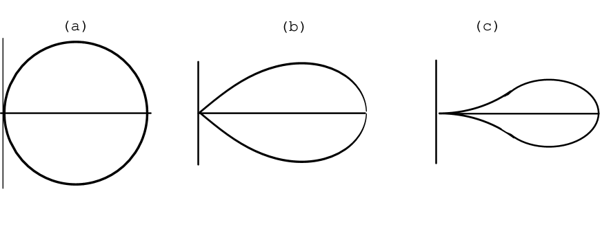
Figure 1: Three summation methods (see Table 2) for three different analyticity and boundedness domains: (a) the disc ${\cal K}(\eta)$, (b) the drop ${\cal L}(\rho)$, and (c) the wedge ${\cal W}$. Crucial is not the size of the domain, but the opening angle at the origin.

Table 2 also shows that the large-order behaviour of the coefficients $a_{n}$ is not the only criterion of the (Borel or some other) summability of the series (21). Even a series with a very tame behaviour of the coefficients $a_{n}$ may not be Borel summable, in spite of the radical suppression of the $a_{n}$ by the Borel factors $1/n!$. An example is discussed in [39].

2.3 Useful facts on power series

Certain important facts on power series are sometimes overlooked in physical considerations. It may therefore be useful to recall some of them here because spontaneous intuition is often misleading. I apologize for some repetition of the text.

1. The divergence of a perturbation expansion does not signal an inconsistency or ambiguity in the theory. An example to illustrate this is the result of Ogievetsky [6], who used the Borel summation method to sum a divergent perturbation series and obtained the exact result derived by Schwinger [5], as is discussed here in subsection 1.1.

The problem is not that of convergence or divergence, but whether the expansion uniquely determines the function or not. The method of Feynman diagrams allows one to find, at least in principle, all coefficients of the perturbation series, which may determine the function uniquely even if the series is divergent, and may not do so even if it is convergent. This depends on additional conditions.

2. The requirement (21) of asymptoticity of a perturbation series is not a formal assumption. It has physical content.

When a perturbation series is divergent, one often re-interprets it automatically as an asymptotic series. This assumption is weaker than that of convergence, but is not self-evident. It is not only technical either. Its physical meaning is that there is a very smooth transition between the system with interaction and the system without it.

For certain classes of observables the perturbation series is believed to be an asymptotic expansion.

3. A very violent behaviour of the expansion coefficients $a_{n}$ at $n\rightarrow\infty$ might make us expect that no function with the property (21) would exist. This fear is not justified; it was proved by Borel and Carleman (see [1] for details) that there are analytic functions corresponding to any asymptotic series.

4. Borel non-summability of a perturbation expansion alone does not signal an inconsistency or ambiguity in the theory. Borel summability (or its lack) is not a fundamental classification criterion (see, e.g., [38, 46]).

While large-order behaviour is often believed to be related to some very deep physics (see [46]), the Borel procedure is just one of many possible summation methods and need not be applicable always and everywhere. There are power series with mildly growing coefficients which are not Borel summable; the problem is to find a method (not necessarily the Borel one) which is appropriate for the case considered.

Example of a non-Borel summable series (although composed of very tamely behaving coefficients) which, nevertheless, is summable by the method based on Theorem 1 is considered in [39] and discussed here in the end of subsection 4.1, (56).

5. If the $a_{n}$ behave very violently at $n\rightarrow\infty$ (so that the Borel series $\sum_{n=0}^{\infty}a_{n}z^{n}/n!$ has zero convergence radius) one might expect that it would be sufficient to replace $n!$ in the denominator by a sequence ${b_{n}}$ that grows faster than $n!$, in order to reach a more efficient suppression of the $a_{n}$. But this is done at a price: stronger conditions on analyticity are required for the summation procedure to be unambiguous.

6. Asymptoticity is not a property of the series alone, but is contingent also upon the properties of the function expanded. These properties (e.g., analyticity) must be examined simultaneously with the asymptotic series, otherwise the same series can be summed to different functions.

7. An asymptotic series need not be divergent. A wide-spread prejudice that gleams, often implicitly, in a number of papers is that an asymptotic series is always a divergent one. To see a quick counterexample, consider the function $F(z)=g(z)+A{\rm e}^{-\alpha/z}$ with $A$ real and $\alpha$ positive, where $g(z)$ is analytic at the origin. This is a two-parametric class of functions $F(z)$ that all have, in the right half plane, the same asymptotic expansion, which is identical with the Taylor series for $g(z)$; so the asymptotic expansion of all the singular functions $F(z)$ is a convergent series because of analyticity of $g(z)$. This convergent series is asymptotic to many singular functions, but its values converge only to one function, the analytic $g(z)$. They do so inside the Taylor circle, which extends up to the nearest-to-origin singularity of $g(z)$.

3 Operator-product expansion and analyticity

3.1 Operator-product expansion

A standard way to investigate the interplay of perturbative and non-perturbative effects is the operator-product expansion (OPE) [49, 51], in which the singularities of an operator product are expressed as a sum of non-singular operators with the coefficients being c-number functions. Being formulated before QCD, the operator-product expansion became a powerful (and actually the only) tool for examining non-perturbative effects in QCD. It consists in expanding the product of two local operators $A(x)$ and $B(y)$, for $(x-y)_{\mu}$ tending to zero, into a series of local operators ${\cal O}_{n}(\frac{1}{2}(x+y))$,

$$A(x)B(y)\approx_{{}_{(x-y)_{{}_{\mu}}\rightarrow 0}}\sum_{n}C_{n}(x-y){\cal O}_{n}((x+y)/2).$$ (29)

where the $C_{n}$ are c-number functions. The meaning of the symbol $\approx$ is discussed below. The operators ${\cal O}_{n}$ are ordered according to their canonical dimensions, and their quantum numbers must match those of $AB$. As a consequence, the coefficients $C_{n}$ are ordered according to their decreasing singularity degree, and only a finite number of them are singular functions infinite at the origin, while the remainder of the expansion is finite or tends to zero with vanishing distance. To any finite order in $x-y$, only a finite number of terms contribute.

The short-distance behaviour of the $C_{n}$ is obtained, by dimensional counting, from

$$C_{n}(x)\rightarrow x^{d_{n}-d_{A}-d_{B}}(\ln xm)^{p}(1+O(xm))$$ (30)

with $d_{A},d_{B}$ and $d_{n}$ being the dimensions of $A,B$ and ${\cal O}_{n}$ respectively, and $m$ being a quantity of the dimension of mass. In this way the canonical dimension of ${\cal O}_{n}$ determines the singularity degree of the corresponding $C_{n}$; the operators ${\cal O}_{n}$ with the smallest dimensions are dominant at short distances, being multiplied with the most singular coefficients $C_{n}$.

In momentum space, the expansion (29) takes the form (we put $y=0$)

$${\rm i}\int{\rm d}x{\rm e}^{{\rm i}qx}A(x)B(0)\approx\sum_{n}C_{n}(q){\cal O}_{n}.$$ (31)

The symbol $\approx$ is understood differently in different contexts.

(i) While originally the validity of OPE was interpreted in the weak sense [49], i.e., in that of sandwiching the product between two fixed states, from the very beginning it has been widely adopted [50] also to understand (29) and (31) as (formal) operator relations.

(ii) Different is the interpretation also in the perturbative and in the non-perturbative context. The standard derivation of OPE [49, 51] relies on an analysis of Feynman graphs and remains within the framework of perturbation theory. The relations (29) and (31) are often understood as asymptotic relations (see, e.g., [52, 53, 54]) which, in special situations (free-field theory, [55]), may become convergent Taylor series.

In application to non-perturbative phenomena, it is assumed [12] that the left- and the right-hand sides of (31) are approximately equal provided that a few first terms are taken. Then, at a critical dimension $d_{r}$, the series breaks down and has to be supplemented with a term which is not of the $Q^{-2k}$ form. At higher values of $k$, other terms of different nature may appear. Relation (31) can be understood as an approximate equality with finite number of terms on the right-hand side [12], with the hope that its validity and practical applicability (far from the point of expansion) can be established by phenomenological analysis of experimental data. Application of this approach to hadron resonances has been very successful; agreement with experimental data and internal consistency of the QCD sum rules scheme are impressive.

Non-perturbative effects manifest themselves also in the fact that, taking the vacuum-to-vacuum matrix element of (31), the terms on the right-hand side can be non-vanishing, whereas only the unit operator would survive within standard perturbation theory.

(iii) Various attitudes are adopted to the topical problem of the validity region (angle, rays) of the expansion (31) in the complex $Q^{2}$ plane. The expansion (31) reflects the properties of the left-hand side at the point of expansion and in a subset of its neighbourhood. In the euclidean ($Q^{2}>0$) region, the expansion is well defined in the sense that the separation of the large-distance contributions from the short-distance ones is well defined [53]. The Minkowski ($Q^{2}<0$) region, on the other hand, is most important for applications, because it contains the spectrum of the physical states.

This indicates that the expansion (31) can have different interpretations, according to the assumed physical content. These interpretations, however, have common mathematical features, which we are going to discuss in the next subsection. We adopt the approach (which is mostly used in phenomenology and is formulated, e.g., in [56]) according to which the operator product expansion is originally built up in the euclidean region and then translated in the language of observables by analytic continuation to the Minkowski region. (For problems of the definition of euclidean Fermi and Bose fields, we refer the reader to [57] and references therein).

Note that along directions in the complex plane away from the euclidean ray different asymptotic expansions may apply or may not exist at all.

Predictions in the Minkowski region are obtained by analytic continuation, which can be carried out under special assumptions of smoothness and stability.

We shall now discuss conditions under which an asymptotic expansion can be extended to angles away from the euclidean semiaxis. It turns out that sign-definitness and integrability of the discontinuity along the cut in the Minkowski region play an important role.

3.2 Operator-product expansion away from euclidean region

The combination of the operator-product expansion with analyticity represents a solid basis for the calculation of the QCD observables. Such calculations require knowledge of the properties of the expansion in the complex energy plane away from the euclidean ray, and analyticity allows one to establish them by means of analytic continuation.

In practical applications of the operator-product expansion one typically meets the following generic situation. Let $f(z)$ be holomorphic in $C$, the complex $z$ plane ($z=1/Q^{2}$), cut along the negative real semiaxis, $z\,\in\,[-\infty,0]$. Let $f(z)$ be bounded by a constant,

$$|f(z)|<M$$ (32)

for $z\,\in\,C$ . Let the numbers $a_{k}$, $k=0,1,2,...n-1$, exist such that the following $n$ inequalities

$$|R_{k}(x)|<N_{k}x^{k}$$ (33)

are satisfied for all $x={\rm Re}z$, $0<x<d$, with $d$ being a positive number, $n$ being a positive integer, and

$$R_{n}(x)=f(x)-\sum_{k=0}^{n-1}a_{k}x^{k}.$$ (34)

The problem is whether or in what sense the estimates (33) apply also to rays away from the positive real semiaxis.

The condition (32) of boundedness by $M$ can be generalized to cases in which the function of interest, $F(z)$, is bounded by a polynomial in $Q^{2}=1/z$ rather than by a constant; the theorem can then be applied either to $F(z)$ multiplied by the corresponding power of $z$, or to the corresponding derivative of $F(z)$.

Notice that our considerations in this section, being equally well applicable to the case of a fixed, finite value of $n$ as well as to the case of $n$ infinite, are not restricted to the case of asymptotic series. We find the case of a finite $n$ closer to physics because, first, one always knows only a finite number of the coefficients $a_{k}$ and, second, theorems dealing with a fixed value of $n$ are more transparent and their application to the case of infinitely many inequalities (33) is straightforward.

The solution to the problem very much depends on the character of the discontinuity of $f(z)$ on the cut.

3.2.1 The case of integrable discontinuity

1. Positive-definite discontinuity. Let us first assume that $f(z)$ can be represented in the form of a generalized Stieltjes integral [59],

$$f(z)=\int_{0}^{\infty}\frac{\rho(t)}{1+zt}{\rm d}t,$$ (35)

where the discontinuity is positive-definite all along the cut, i.e., $\rho(t)$ is nonnegative for $t>0$. Let $\rho(t)$ be such that the integral in (35) exists for $z$ complex, not negative, and that also the moments

$$a_{k}=\int_{0}^{\infty}t^{k}\rho(t){\rm d}t$$ (36)

exist for all nonnegative integers $k$.

The function $f(z)$ has an asymptotic power expansion with the coefficients $(-1)^{k}a_{k}$,

$$f(z)\sim\sum_{k=0}^{\infty}(-1)^{k}a_{k}z^{k}$$ (37)

for $z$ approaching zero from the positive side, $z\rightarrow 0_{+}$. Indeed,

$$R_{n}(z)=(-z)^{n}\int_{0}^{\infty}\frac{\rho(t)}{1+zt}t^{n}{\rm d}t$$ (38)

and, consequently,

$$|R_{n}(z)|=\tilde{a}_{n}(z)|z|^{n}\leq a_{n}|z|^{n}$$ (39)

which, as expected, tends to zero one order faster than $|z|^{n-1}$, the highest power subtracted from $f(z)$ (see (34)). We use the notation

$$\tilde{a}_{n}(z)=\int_{0}^{\infty}\frac{\rho(t)}{|1+zt|}t^{n}{\rm d}t.$$ (40)

Analogous estimates are obtained for $z$ approaching zero along a ray in the complex plane (but away from the Minkowski ray). In the right halfplane, certainly, $\tilde{a}_{n}(z)\leq a_{n}$ , but this is not the case for Re $z<0$, where the general bound on $\tilde{a}_{n}(z)$ is worse, due to the presence of the cut in this halfplane. The bound can be obtained as follows. We have, denoting $z=r{\rm e}^{{\rm i}\phi}$,

$$|1+zt|=(1+2rt\cos\phi+r^{2}t^{2})^{1/2}.$$ (41)

Considered as a function of $t$ at $t>0$ and $\phi$ fixed, $1/|1+zt|$ has its maximum at $t=t_{0}=-\frac{1}{r}\cos\phi$, where its value is $1/|\sin\phi|$. In this way we obtain (39) and

$$|R_{n}(z)|\leq\frac{1}{|\sin\phi|}\,a_{n}\,|z|^{n}$$ (42)

for Re$\,z>0$ and Re $z<0$ respectively. Comparing (42) with (39), we see how the factor $1/|\sin\phi|$ makes the estimate looser when the ray approaches the direction of the cut, i.e., when $\phi$ approaches zero.

Possible applications to some QCD processes are discussed in subsection 5.2.

2. Sign-indefinite discontinuity. The estimates are worse if the discontinuity along the cut is not positive definite. Physical relevance of such situations is pointed out in [53]. If the integral representation (35) is still admitted, be it with $\rho(t)$ sign-indefinite or even a complex-valued function on the integration interval, the resulting bounds (39) and (42) have to be modified in the following sense. The function $\rho(t)$ is assumed to be such that the integral (35) is absolutely convergent and that the moments of $|\rho(t)|$ ,

$$\bar{a}_{k}=\int_{0}^{\infty}t^{k}|\rho(t)|{\rm d}t,$$ (43)

are convergent integrals; this excludes wild oscillations of the discontinuity along the cut. The estimates (39) and (42) are replaced by

$$|R_{n}(z)|\leq\bar{a}_{n}\,|z|^{n}$$ (44)

and

$$|R_{n}(z)|\leq\frac{1}{|\sin\phi|}\,\bar{a}_{n}\,|z|^{n}$$ (45)

respectively. This may imply a considerable deterioration of the estimate relative to a sign-definite $\rho(t)$: if the discontinuity on the cut oscillates, $\bar{a}_{n}$ and $|R_{n}(z)|$ will have very little to do with the expansion coefficient $a_{n}$.

Better estimates on $|R_{n}(z)|$ than (39), (42) and, respectively, (44), (45) cannot be obtained unless some special assumptions are made about the explicit form of the function $\rho(t)$ in the respective cases.

3.2.2 General case

It is interesting to discuss a further generalization, although its relevance for physics may still be unclear. In the general case, when the integral (35) is not absolutely convergent or the moments (43) are not defined, we can use a theorem by I. Vrkoč (see [41]) to obtain an estimate. Assumed are holomorphy of $f(z)$ and the bound (32) on $f(z)$ to be valid in an angle $2\alpha$ bisected by the real axis, and the inequality

$$|R_{n}(x)|<N_{n}x^{n}$$ (46)

to hold for a positive integer $n$ and for $0<x<d$. When applied to $\alpha=\pi$ (the values of $n$ and $d$ being fixed), the theorem implies that, along all rays between $-\pi(1-2^{-l})$ and $\pi(1-2^{l})$, $R_{m}(z)$ satisfies the following inequality:

$$|R_{m}(z)|<\hat{N}_{m}|z|^{n/2^{l}}$$ (47)

for all $|z|<d_{0}$, where $d_{0}$ is a positive number and $l$ is a nonnegative integer. The coefficient $\hat{N}_{m}$ in front of $|z|^{n/2^{l}}$ is a linear combination of the $|a_{k}|$ for $k$ running from $m=[(n-1)/2^{l}]+1$ to $n-1$, $[q]$ denoting the integer part of the real number $q$.

This result is of relevance for expansions both with a finite and with infinite number of terms. Note that the bound (46) on $R_{n}(x)$ for $x$ positive implies, for $z$ complex, the estimate (47) on $R_{m}(z)$, where $m$ is smaller than $n$. This resulting bound for complex $z$ is considerably looser than that for $x$ real, the number of exploitable terms being reduced from $n$ down to $m=[(n-1)/2^{l}]+1$. This effect is the price paid for the extended validity region of (47), and is becoming more and more pronounced with increasing $l$, i.e., with increasing angular deflection from the euclidean interval. We also see that the higher-order expansion coefficients $a_{k}$ (for $k=m+1,..,n-1$) cannot be used to improve the bound along a complex ray.

The result shows quantitatively how quickly the expansion breaks down when the angle becomes large, i.e., when one approaches the cut on the Minkowski side of the real axis. As is usual in analytic extrapolations [60], a point-by-point continuation from approximate data is impossible, and an extrapolation up to the cut can be safely done onto an interval but not to a point. The procedure should be based on statistical analysis of experimental data, [61].

Since the estimate (47) might seem rather loose (note that $n$ in the exponent on the right hand side is divided by $2^{l}$), it is interesting to look for a function which would saturate it. A set of functions saturating (47) for different nonnegative integers $n$ can be generated by using the function $\exp(-{\rm i}a(\ln z)^{2})$ with $a$ real.

Further modifications of the results of this section will arise when the logarithmic dependence of the expansion coefficients $C_{n}(x)$ indicated in (30) is taken into account. Physical relevance of this generalization is evident.

4 Renormalons and instantons

4.1 Singularities in the Borel plane

The integral (14) defines the Borel sum of the series (12) if the conditions 1), 2) and 3) from subsection 2.1 are satisfied.

The condition 1) would be violated if the $a_{n}$ were to grow faster than $n!$. As follows from Table 1, this is not the case in typical situations.

We generally do not know the nature or distribution of singularities to assess the validity of the condition 2). Analyses of large-order behaviour indicate that 2) is violated by an infinite set of singularities located on the real axis (renormalons, instantons). Then, the integral (14) is not well-defined and should not be used. In quantum theory, however, it is nevertheless used, with the aim to reduce the problem of summation to that of defining the integral (14) by means of a suitable modification of the integration contour.

The spectrum of ambiguitites is wider, however. By introducing the renormalon language we consider only special sets of equidistant singularities (poles, branch points) whose parameters have physical interpretation. Those lying on the positive real semiaxis produce ambiguity and remind us that non-perturbative input has to be added.

The electromagnetic current–current correlation function is a useful example to discuss a typical structure of singularities in the complex coupling-constant plane. Denoting this function $\Pi^{\mu\nu}$,

$$\Pi^{\mu\nu}={\rm i}\int{\rm d}^{4}x{\rm e}^{-{\rm i}qx}\langle 0|\,{\rm T}(j^{\mu}(x)j^{\nu}(0))\,|0\rangle$$ (48)

$$=(g^{\mu\nu}q^{2}-q^{\mu}q^{\nu})\Pi(-q^{2})$$ (49)

and taking $R$, the ratio of the total cross section for ${\rm e}^{+}{\rm e}^{-}\rightarrow{\rm hadrons}$ to that for ${\rm e}^{+}{\rm e}^{-}\rightarrow\mu^{+}\mu^{-}$, which is related to the imaginary part of $\Pi$,

$$R(s)=12\pi{\rm Im}\,\Pi(s+{\rm i}0^{+})\,,$$ (50)

we introduce a modified quantity $D(Q^{2})$ defined as

$$D(Q^{2})=-4\pi^{2}Q^{2}\left(\frac{{\rm d}}{{\rm d}Q^{2}}\right)\Pi(Q^{2})$$ (51)

(where $Q^{2}=-q^{2}$, i.e., $Q^{2}>0$ in the euclidean domain), to avoid inessential logarithmic terms and the dependence on the renormalization scale $\mu$ [64]). The perturbation expansion of $D$ in powers of the coupling constant has the form

$$D\sim 1+\frac{\alpha_{s}(Q^{2})}{\pi}\sum_{n=0}^{\infty}D_{n}(\alpha_{s}(Q^{2}))^{n}.$$ (52)

The dependence of $D$ on $\alpha_{s}(Q^{2})$ exhibits a complex structure of singularities in the coupling constant plane at and around the origin [9]. Their nature can be conveniently displayed by studying the corresponding Borel transform. The behaviour of the running coupling constant $g(\mu^{2})$ is determined by the $\beta$ function, $\beta(g^{2}(\mu^{2}))\equiv\mu^{2}({\rm d}/{\rm d}\mu^{2})g^{2}(\mu^{2})$, which has the perturbative expansion $\beta(g^{2})\sim-b_{0}g^{4}-b_{1}g^{6}-...\,$.

The structure of the singularities of the Borel transform that are nearest to the origin can be seen from the following (simplified, see [48, 62]) expression for $D$

$$Q^{2}\int{\rm d}k^{2}\frac{k^{2}\alpha_{s}(k^{2})}{(k^{2}+Q^{2})^{3}},$$ (53)

which at the infrared and the ultraviolet end of the spectrum has the following behaviour

$$\alpha_{s}(Q^{2})\sum_{n}[b\alpha_{s}(Q^{2})/(4\pi)]^{n}n!/2^{n+1}$$ (54)

and

$$\alpha_{s}(Q^{2})\sum_{n}[-b\alpha_{s}(Q^{2})/(4\pi)]^{n}n!$$ (55)

respectively, where $b$ is the first coefficient in the Gell-Mann–Low function. This corresponds to an $n!$ large-order behaviour, with the nearest singularities located in the Borel plane at $8\pi/b$ and $-4\pi/b$ respectively.

Perturbation theory suggests the following structure of the singularities of the Borel transform [64, 48]:

(1) Instanton–anti-instanton pairs [18, 19] generate equidistant singularities along the positive real axis starting at $t=4$, for $t=4l,l=1,2,...$. Balitsky [65] calculated the behaviour of $R_{{\rm e}^{+}{\rm e}^{-}\rightarrow{\rm hadrons}}$ near $t=4$ and found the leading ${\rm I-{\bar{I}}}$ singularity to be a branch point with the power $\frac{11}{6}(N_{\rm f}-N)$, where $N$ and $N_{{\rm f}}$ is the number of colours and of flavours respectively.

(2) Ultraviolet renormalons are generated by contributions behaving as $c_{k+1}\sim(-b_{0}/l)^{k}k!$ for $l=1,2,...$, leading to singularities located at $t=-2l/b$   on the negative real axis (where $b=8\pi^{2}b_{0}$), with a branch point for $l=1$.

(3) Infrared renormalons are generated by contributions behaving as $c_{k+1}\sim(b_{0}/l)^{k}k!$, $l=2,3,...$, leading to singularities located at $t=2l/b$. Near the first of the points, the singularity behaves [11] as $(bt-4)^{-1-2\lambda/b_{0}}$, $\lambda=b_{1}/b_{0}$. By absence of a dimension-two condensate the existence of the $l=1$-singularity is excluded.

Other singularities are not assumed to exist in the Borel plane. But there may be still another source of ambiguities, due to possible singularities at infinity. They may be non-Borel summable, no matter how tame the large-order growth may be! A trivial example is the series $\sum_{n=0}^{\infty}z^{n}$, whose coefficients are constant. It has no singularities in the Borel plane, but the series is Borel summable only for Re$z<1$, because otherwise the Borel integral does not exist. A more sophisticated example is $\sum_{n=0}^{\infty}c_{n}z^{n}$ with

$$c_{n}=c^{n}\mu(n)$$

$$\mu(n)=\int_{0}^{\infty}{\rm exp(-e}^{t})\,\,t^{n}{\rm d}t$$ (56)

$$c=|c|{\rm e}^{{\rm i}\theta},\,\,\,\,\,0<\theta<\pi/2$$

(see ref. [39], Example 3). Note the double exponential in the integrand, which makes $\mu(n)$ and $c_{n}$ rise extremely slowly. At first sight, this series should be Borel summable, even more that there are no singularities in the Borel plane, the convergence radius (condition 2)) being infinity. But the condition 3) is not satisfied: the integral (14) does not exist. Indeed,

$$\int_{0}^{\infty}{\rm d}t{\rm e}^{-t/z}\sum_{n=0}^{\infty}\frac{c_{n}}{n!}t^{n}$$ (57)

is divergent, because $B(t)$ grows faster than ${\rm e}^{t}$ with $t\rightarrow+\infty$. But the series $\sum_{n=0}^{\infty}c_{n}z^{n}$ is summable by Moroz’s method [38].

4.2 A further generalization of Borel transformation

The functions $B_{\rho}(t)$ and $M(t)$ defined in Table 2 are generalizations of the Borel transform, which can be used in the various situations listed in Table 1 to reduce non-uniqueness, provided some additional information is available. More about the properties of $B_{\rho}(t)$ and $M(t)$ can be found in [38, 39, 40, 42] and in references therein.

I will now discuss another type of generalization of the notion of Borel transform, [63, 64, 47], which makes use of the specific structures mentioned in the previous subsection.

Let me first make a general remark. After having exposed mathematical methods in sections 1 and 2, we have passed to practical aspects of the operator-product expansion (estimate of the remainder after the $n$-th term, see section 3), and of the assumption (in section 4) that two-point Green’s functions have special singularities in the Borel plane, the instantons and the renormalons, a structure that is now almost universally adopted. Existence of these structures in the Borel plane is based on various mathematical models developed in late 70’s and early 80’s, but nowadays they are mostly considered as true features of Nature.

Brown, Yaffe and Zhai and Beneke [63, 64, 47] use information about the structure of the first infrared renormalon. Assuming first the special case of a one-term $\beta$ function,

$$\beta(g^{2})=-b_{0}\,g^{4}\,,$$ (58)

expanding ${\rm Im}\,\Pi$ and $\Pi$ in powers of the coupling constant with the expansion coefficients $a_{n}$ and $c_{n}$ respectively and defining their respective Borel transforms

$$A(t)=\sum_{n=1}^{\infty}\frac{na_{n}}{\Gamma(n+1)}\,t^{n}$$ (59)

and

$$C(t)={\tilde{c}_{0}}+\sum_{n=1}^{\infty}\frac{nc_{n}}{\Gamma(n+1)}\,t^{n}\,,$$ (60)

Brown and Yaffe [63] obtain, by comparing the expansion coefficients, the following relation between $A$ and $C$:

$$A(t)=\sin(b_{0}t)C(t)\,,$$ (61)

which turns out to be a consequence of renormalization-group invariance [47]. Defining a modified Borel transform ${\cal F}(t)$ by

$${\cal F}(t)=\sum_{n=0}^{\infty}\frac{\Gamma(1+\lambda t)}{\Gamma(n+1+\lambda t)}f_{n}t^{n}$$ (62)

(thereby accounting for the first infrared renormalon), the authors of [64, 47] consider the case of a general beta function, chosen in such a scheme that its inverse contains two terms:

$$1/\beta(g^{2})=-1/(b_{0}g^{4})+\lambda/(b_{0}g^{2}).$$ (63)

They find that, for this form of $\beta(g^{2})$, the relation (61) remains valid also for ${\cal A}(t)$ and ${\cal C}(t)$, the modified (according to (62)) Borel transforms of ${\rm Im}\,\Pi$ and $\Pi$ respectively:

$${\cal A}(t)=\sin(b_{0}t)\,{\cal C}(t)\,.$$ (64)

In this way, the endeavour to retain the relation (61) also for the case of a general $\beta$ function motivates the authors to introduce the generalized Borel transform in the form (62).

It was already pointed out that the concept of renormalon is at present applied to concrete physical situations. This poses a topical problem: To what extent are renormalons physical concepts and to what extent are they just artefacts of our, maybe inadequate, formalism? Some authors [66] argue that the series of renormalon-type graphs is ill-defined, or that infrared renormalons might be an attribute of the renormalization scheme used. The Borel plane formalism is, nevertheless, successful in phenomenology.

4.3 Phenomenology in the Borel plane

Soper and Surguladze [67] use information on the singularities in the Borel plane to compute the ratio $R$ of the width for Z$\rightarrow$ hadrons to that for Z$\rightarrow$ e⁺e^-. The result is impressive. Considering $R$ as a function $R(s)$ of $s$, the c.m. energy squared of the e⁺e^- annihilation, one obtains the measured $R$ as $R(M^{2}_{{\rm Z}})$. Representing $R(s)$ and $D(s)$ as $R_{0}[1+{\cal R}(s)]$ and $D_{0}[1+{\cal D}(s)]$ respectively with ${\cal R}$ and ${\cal D}$ expanded in powers of the coupling constant $\alpha_{s}(s)/\pi$, the authors of [67] use, in view of the relations (50) and (51), the formula

$${\cal R}(s)=\frac{1}{2\pi}\int_{-\pi}^{\pi}{\rm d}\theta{\cal D}(s{\rm e}^{{\rm i}\theta})$$ (65)

to calculate ${\cal R}(s)$ from ${\cal D}(z)$. Both ${\cal R}$ and ${\cal D}$ are expanded in perturbation series to third order, where the coefficients are explicitly known. Assuming now a standard large-order behaviour of the perturbative expansion of ${\cal D}$, the authors write the Borel representation for it,

$${\cal D}(Q^{2})=\int_{0}^{\infty}{\rm d}z\exp(-\pi z/(\alpha_{s}(Q^{2}))\tilde{\cal D}(z),$$ (66)

where the Borel-transform coefficients $\tilde{\cal D}_{n}$ have better large-order behaviour than the ${\cal D}_{n}$, those of the original series. Combining (65) with (66), one expresses ${\cal R}$ directly in terms of $\tilde{\cal D}(z)$ through an integral over $z$ from 0 to $\infty$, in which the upper limit can be safely replaced by $z_{{\rm max}}$, with $\beta_{0}z_{{\em max}}$ around 0.5 or higher. The ultraviolet renormalon at $\beta_{0}z=-1$, being the singularity closest to the origin, controls the large-order behaviour of the perturbative series; the authors of [67] move it farther by means of the conformal mapping

$$\beta_{0}(\zeta)=4\frac{\sqrt{1+\beta_{0}z}-1}{\sqrt{1+\beta_{0}z}+1}\,\,,$$ (67)

thereby improving the convergence rate of the power series in the Borel plane. Note that the other set of dangerous singularities, the infrared renormalons (the nearest of which is at $\beta_{0}z=+2$), are not pushed away from the origin by (67), but on the contrary become closer to it. Although the infrared renormalons could be pushed away by means of the optimal conformal mapping [68] (which leads to the fastest convergence), Soper and Surguladze [67] prefer to soften the nearest infrared renormalon by multiplying $\tilde{\cal D}$ with its power, because they know the numerical value of the exponent. Making good use of this valuable piece of information, they reach a high accuracy in determining $\alpha_{s}(M^{2}_{{\rm Z}})$, estimating that the uncertainty arising from QCD is less than 0.5 per cent.

4.4 Renormalons and OPE

A scheme to use renormalons to construct non-perturbative terms in the operator-product expansion has been proposed by Grunberg [69]. Defining from $\Pi(Q^{2})$ the renormalization-group invariant quantity

$$R(Q^{2})=\frac{{\rm d}\Pi}{{\rm d}\ln Q^{2}}-\frac{{\rm d}\Pi}{{\rm d}\ln Q^{2}}|_{\alpha=0},$$ (68)

he uses the OPE representation

$$R(Q^{2})=R_{{\rm PT}}(\alpha)+G_{0}(\alpha)+...,$$ (69)

where $\alpha=\alpha(\mu)$ is the coupling at scale $\mu$, $R_{{\rm PT}}(\alpha)=\sum_{n=0}^{\infty}r_{n}\alpha^{n+1}$ the perturbative contribution and $G_{0}(\alpha)$ is the leading condensate contribution. For $G_{0}(\alpha)$, the renormalization group equation yields

$$G_{0}(\alpha)=C(\mu^{2}/Q^{2})^{d/2}\exp(d/(2\beta_{0}\alpha))\alpha^{\delta}[1+O(\alpha)],$$ (70)

where $\delta$ is expressed through the $\beta$-function coefficients, and the $\mu$-dependence of the factor $(\mu^{2}/Q^{2})^{d/2}$ is compensated by that of the subsequent exponential function.

The function $R_{{\rm PT}}(\alpha)$ is then approximated by first infrared renormalon singularity. Using the Borel representation

$$R_{{\rm PT}}(\alpha)=\int_{0}^{\infty}{\rm d}z\exp(-z/\alpha)R^{\rm B}_{\rm PT}(z)$$ (71)

with $R^{{\rm B}}_{{\rm PT}}(z)$ approximated by the first renormalon $R^{{\rm B}}_{{\rm PT,0}}(z)$,

$$R^{{\rm B}}_{{\rm PT,0}}(z)=K(\mu^{2}/Q^{2})^{-z_{0}\beta_{0}}(1-z/z_{0})^{-\gamma}[1+O(1-z/z_{0}],$$ (72)

where $K$ is a scale-independent factor, Grunberg arrives [69] at

$${\rm Im}R_{{\rm PT,0}}(\alpha)=\pm Kz_{0}^{\gamma}\Gamma(1-\gamma)\sin(\pi(1-\gamma))(\mu^{2}/Q^{2})^{-z_{0}\beta_{0}}\exp(-z_{0}/\alpha)\alpha^{1-\gamma}[1+O(\alpha)].$$ (73)

The sign depends on the choice of the integration contour; thus, the resummed $R_{{\rm PT}}(\alpha)$ cannot determine $R$ uniquely. Consistency requires the ambiguity to be removed by some non-perturbative input. Assuming $C$ in (70) complex, Grunberg [69] compares (73) with (70) to find relations connecting $z_{0}\beta_{0}$ and $\gamma$ with $d$ and $\delta$ and to fix the position and the power of the singularity.

This method allows non-perturbative terms in the operator-product expansion to be constructed from perturbation theory. The author gives a convergent scheme to deal with perturbation theory in presence of infrared renormalons. The procedure can be extended to non-leading IR renormalons.

Grunberg’s result shows that there are “non-perturbative” terms in the operator-product expansion which have their origin in perturbation theory. The author considers also the possibility that all “non-perturbative terms” in the expansion, taken to all orders, could be determined in principle from perturbation theory. This interesting possibility could be a good starting point for approximations, although it does not mean that all QCD could be fully described in terms of perturbative concepts. Within perturbation theory one can account for the infrared domain up to terms of the form

$$\exp(m/(\beta_{0}\alpha(Q))\sim(\Lambda^{2}/Q^{2})^{m}$$ (74)

(see a discussion in [70]), where $m$ is the order of IR renormalon. On the other hand, an additional non-perturbative input may also have implications in the Borel plane. The presence of renormalons can signal deficiency of the perturbative approach and indicate a nonperturbative supplement.

5 Further applications

5.1 Resummation of bubble chains

The renewed interest in calculating higher-order perturbative corrections and in examining the high-order behaviour of perturbative series is intimately related to the investigation of renormalization scale and scheme dependence of a truncated series as well as to attempts to estimate its uncalculated remainder. In the past various criteria for finding a suitable renormalization prescription were proposed; they are based on an estimate of the size of the remainder. Examples are Stevenson’s principle of minimal sensitivity [4], Grunberg’s notion of effective charge [71], and the BLM method of scale setting [72] by Brodsky, Lepage and Mackenzie. The BLM prescription, which is based on an analogy with QED, was further developed recently. It is a method of estimating higher-order perturbative corrections of a physical quantity, provided that the first approximation is known. It consists in the use of some “average virtuality” as scale in the running coupling. Instead of working with fixed scale,

$$\alpha_{s}(Q^{2})\int{\rm d}^{4}kF(k,Q)\,,$$ (75)

one averages over the logarithm of the gluon momentum:

$$\alpha_{s}(Q_{BLM}^{2})\int{\rm d}^{4}kF(k,Q)\equiv\alpha_{s}(Q^{2})\int{\rm d}^{4}k\left(1-\frac{\beta_{0}}{4\pi}\alpha_{s}(Q^{2})\ln\frac{-k^{2}}{Q^{2}}\right)F(k,Q)\,.\,\,\,$$ (76)

This replacement amounts to accounting for higher-order terms in powers of $\alpha_{s}(Q^{2})$ by making use of the renormalization-group evolution

$$\alpha_{s}(-k^{2})=\alpha_{s}(Q^{2})\sum_{n=1}^{\infty}\left(\frac{\beta_{0}\alpha_{s}(Q^{2})}{4\pi}\right)^{n-1}(-\ln(-k^{2}/Q^{2}))^{n-1}$$ (77)

(in the leading-logarithm approximation) and retaining only the first two terms in the sum. This approach was generalized [73, 80, 81] by introducing the running coupling constant $\alpha_{s}(k^{2})$ directly into the vertices of Feynman diagrams, with $k$ being the momentum “flowing” through the line of the virtual gluon. This modification means replacement of (76) by

$$\alpha_{s}(Q^{*2})\int{\rm d}^{4}kF(k,Q)=\int{\rm d}^{4}k\alpha_{s}(-k^{2})F(k,Q)\,\,\,$$ (78)

with $\alpha_{s}(x^{2})=4\pi/(\beta_{0}\ln(x^{2}/\Lambda^{2}_{QCD})$. Note, however, that the beta function $\beta(\alpha_{s}(Q^{2}))$ is approximated by its first term only.

This method has been applied in phenomenology to various QCD observables, such as $\tau$ decay hadronic width and heavy-quark pole mass [83, 81], semileptonic B-meson decay [82] and the Drell–Yan process [83]. It makes maximal use of the information contained in the one-loop perturbative corrections combined with the one-loop running of the effective coupling, thereby providing a natural extension of the BLM scale-fixing prescription.

Methods generalizing the scale-setting procedure developed by Brodsky, Lepage and Mackenzie met with criticism [84, 85] showing that the summation based on “naive non-abelization” is renormalization-prescription dependent. Further research will clarify the issue; some of its aspects are discussed in Sec. 6.

A resummation that is renormalization-scheme invariant in the large-$N_{f}$ approximation has recently been proposed by Maxwell and Tonge [86]. It is based on approximating the effective charge beta-function coefficients by the part produced by the highest power of $b=(11N_{c}-2N_{f})/6$, and accounts for exact all-orders results in this approximation. This method allows one to include, in any renormalization scheme, the exact perturbative coefficients not only at NLO but also at NNLO. The approach is used to critically examine the reliability of calculations of fixed-order perturbation theory for various observables and sum rules. Application of the RS-invariant resummation to different physical processes indicates varying reliability of the standard fixed-order perturbation theory.

Ellis et al. [87] use Padé approximants to develop another method of resumming the QCD perturbative series. The authors test their method on various known QCD results and find that it works very well; in particular, they reach a weaker renormalization-scale dependence of the calculations. The problem why Padé approximants reduce the renormalization-scale dependence has recently been considered in ref. [88]. The author finds that in the “large $\beta_{0}$ limit” (when the beta function is dominated by the 1-loop contribution) diagonal Padé approximants become renormalization-scale independent, thereby sharing an important feature of the exact result.

5.2 Use of operator-product expansion

Operator-product expansion has proved to be very useful in practical calculations in connection with the tau decay hadronic width, the heavy quark pole mass, heavy-light quark systems, semileptonic B-meson decay, heavy quarkonia and the Drell-Yan process. Renewed interest in the evaluation of power corrections to QCD predictions has resulted in attempts to understand the implications of the presence of renormalon singularities in these processes.

Starting from analyticity and operator product expansion Braaten, Narison and Pich [89] used the measurements of the $\tau$ decay rates to determine the QCD running coupling constant at the scale of the $\tau$ mass $M_{\tau}$=1.784 GeV. The ratio $R_{\tau}$,

$$R_{\tau}=\frac{\Gamma[\tau^{-}\rightarrow\nu_{\tau}{\rm hadrons}(\gamma)]}{\Gamma[\tau^{-}\rightarrow\nu_{\tau}{\rm e}^{-}\bar{\nu}_{\rm e}(\gamma)]}$$ (79)

(where $(\gamma)$ represents possible additional photons or lepton pairs), is represented in the form

$$12\pi\int_{0}^{M_{\tau}^{2}}(1-s/M_{\tau}^{2})^{2}(1+2s/M_{\tau}^{2}){\rm Im}\Pi(s)\frac{{\rm d}s}{M_{\tau}^{2}}$$ (80)

where $\Pi(s)$ is a combination of the two-point correlation functions for the vector $V_{ij}^{\mu}=\bar{\psi}_{j}\gamma^{\mu}\psi_{i}$ and axial vector $A_{ij}^{\mu}=\bar{\psi}_{j}\gamma^{\mu}\gamma_{5}\psi_{i}$ colour singlet quark currents, with coefficients given by the elements $V_{{\rm ud}}$ and $V_{{\rm us}}$ of the Kobayashi-Maskawa matrix, the subscripts $i,j=$u,d,s denoting light quark flavours.

This integral cannot at present be calculated from QCD, because the hadronic functions are sensitive to the non-perturbative effects that confine quarks in hadrons. But one can make use of the properties of the correlating functions, which are known to be analytic in the complex $s$-plane cut along the positive real semiaxis. This allows the integral in (80) to be expressed as a contour integral along the circle of radius $M_{\tau}^{2}$:

$$6\pi{\rm i}\oint_{|s|=M_{\tau}^{2}}(1-s/M_{\tau}^{2})^{2}(1+2s/M_{\tau}^{2})\Pi(s)\frac{{\rm d}s}{M_{\tau}^{2}}\,.$$ (81)

Representing now $\Pi(s)$ as the operator product expansion over local gauge invariant operators, the authors of [89] point out that the double zero in the kinematic factor of the integrand at $s=M_{\tau}^{2}$ suppresses the contribution from the dangerous segment close to the branch cut, where OPE has little chance to represent appropriately the function. (As a further means of suppressing bad influence of this segment, integral averaging smeared over an energy of the order $\Lambda_{{\rm QCD}}$ can be used.) Application of the estimates discussed in subsection 3.2 will give quantitative background to this qualitative assumption, specifying how reliable the expansion is at the points $|s|=M_{\tau}^{2}$ that are far both from the euclidean interval and from the immediate neighbourhood of the point $s=M_{\tau}^{2}$, thereby possibly modifying the accuracy of some of the estimates.

The estimate of $\alpha_{s}$ and of the QCD condensates from e⁺e${}^{-}\rightarrow I=1$ data was re-examined in [90] using $\tau$-like inclusive process and QCD sum rules. The resulting values confirm previous sum rules estimate based on stability criteria. Implication on the value of $\alpha_{s}$ from $\tau$-decays gives 0.33 $\pm$ 0.03 as the value of $\alpha_{s}(M_{\tau})$.

Applications of the operator-product expansion to heavy quark physics (such as B and $\Lambda_{{\rm b}}$ decays, the problem of heavy-quark pole mass) are based on an extension of the idea of the operator-product expansion to a new situation, when the expansion is made in terms of operators in the heavy-quark effective field theory, in inverse powers of a quantity of the scale of the heavy quark mass $m_{{\rm Q}}$ [76]. Heavy-quark field theory is, to leading order, a theory for light quarks in the field of a static colour source. Evidently, $m_{{\rm Q}}$, this key quantity, is not uniquely defined because quarks are unobservable; the so-called pole mass $m_{{\rm Q}}^{{\rm pole}}$ (i.e., the position of the pole in the quark propagator) is well-defined in each finite-order perturbation theory [62] but, as the authors show, no precise definition of the pole mass exists once nonperturbative effects are included. They argue that any consistent definition of this quantity suffers from an intrinsic uncertainty of order [pole mass times $\Lambda_{{\rm QCD}}/m_{\rm Q}$]. This circumstance can be described in terms of an infrared renormalon of the type (54), which produces a factorial divergence of the perturbation series.

As in the $\tau$ decay case, also in the case of the heavy-quark systems the approach starts from the operator-product expansion in euclidean region, this time in the kinematic invariant $v.q$, where $v$ is the velocity of the heavy quark. Again, the problem leads to a contour integral of the type (81), which has a segment close to the cut, where the expansion is not safe, and it is expected that smearing over an energy of the order $\Lambda_{{\rm QCD}}$ would make valid the OPE computation of the differential distributions. Results for semileptonic B and $\Lambda_{{\rm b}}$ decays are obtained in [76].

The relation of the heavy quark mass to the expansion parameter is investigated in [70]. It is shown that the heavy-quark effective theory suffers from a series of ultraviolet renormalons which are not Borel-summable. The heavy-quark effective theory should be independent of the heavy-quark mass; since the $S$-matrix elements in a confining theory have no poles corresponding to a physical quark there is no natural choice of the expansion parameter. The ambiguity of perturbation series is related to an infrared renormalon in the pole mass and expresses the necessity of including an additional (and ambiguous) mass term.

The structure of renormalons in the heavy-quark effective theory is examined in [77]. The authors show that the way in which renormalons appear in effective theories is not universal, but depends on the regularization scheme used to define the effective theory. In the case of kinetic energy operator, they find that the leading ultraviolet renormalon is absent in all but one regularization schemes.

The authors of [78] develop a nonperturbative method for defining the higher-dimensional operators of the heavy quark effective theory such that the matrix elements are free of ambiguities due to the UV renormalon singularities. They define a ”subtracted pole mass” from which the renormalon singularities are subtracted in a nonperturbative way and whose inverse can be used as the expansion parameter.

For a critical review of recent achievements in the heavy quark theory see ref. [79].

6 Renormalization ambiguities

Results of any finite-order calculation depend on the renormalization prescription, although the theory as a whole must be invariant with respect to the renormalization group. This issue has been lively discussed in QCD since many years in connection with theoretical predictions of observable quantities. As the renormalization-group dependence of a finite-order result can never be fully removed, the effort has been focused on looking for such a renormalization prescription (RP) and such a method of approximation which would possibly minimize the dependence on the choice of the RP. The extent of ambiguities connected with renormalization-group invariance is often not fully appreciated; we shall therefore explain the main concepts and the actual origin of the ambiguities. In expounding the subject we shall follow the way outlined in ref. [84]; for practical aspects of the renormalization scheme dependence of the perturbative QCD approximations see also [91], [92].

Let $r(Q)$ be a generic observable quantity that depends, for simplicity, on a single external momentum $Q$,

$$r(Q)=a\left[1+r_{1}a+r_{2}a^{2}+...\right].$$ (82)

On the right-hand side, the $Q$-dependence of $r(Q)$ is hidden in a $Q$ dependence of the expansion coefficients $r_{k}$. Besides this, both $a$ (the renormalized coupling constant, often called coupling parameter or couplant in this context, to emphasize its running character) and the coefficients $r_{k}$ depend on the renormalization prescription (RP), which consists of the choice of the renormalization scale $\mu$ (of dimension energy) and of the so-called renormalization scheme (RS). Thus,

$$a=a(\mu,{\rm RS})$$

$$r_{k}=r_{k}(Q/\mu,{\rm RS}).$$ (83)

The quantity $r(Q)$, on the other hand, should not (by definition) depend on $\mu$ or RS, because it is an observable quantity.

One can distinguish the following stages of fixing the renormalization-group ambiguities.

1. Renormalization scale. The dependence of the couplant $a$ on the scale $\mu$ is governed by the differential equation

$$\frac{{\rm d}a(\mu,{\rm RS})}{{\rm d}\ln\mu}\equiv\beta(a)=-ba^{2}(\mu,{\rm RS})\left(1+ca(\mu,{\rm RS})+c_{2}a(\mu,{\rm RS})+...\right).$$ (84)

The choice of the renormalization scale consists in selecting, when equation (84) has been solved, the value of the parameter $\mu$, with respect to which the theory is invariant.

2. Renormalization convention. While $b$ and $c$, the first two coefficients on the right hand side of (84), are uniquely determined as functions of $N_{f}$ and $N_{c}$,

$$b=(11N_{c}-2N_{f})/6$$

$$c=(51N_{c}-19N_{f})/(11N_{c}-4N_{f})$$

(where $N_{f}$ and $N_{c}$ is the number of massless quark species and the number of colours respectively), all the other coefficients $c_{i}$ are completely arbitrary and define the renormalization convention, see Table 3. One can consider different renormalization conventions (i.e., different choices of the $c_{i}$), among which ’t Hooft’s convention [9], in which all the $c_{i}$ vanish, is remarkable for its simplicity and is suitable for general considerations; in this convention, the right-hand side of (84) consists of two terms, while (82) is generally an infinite series. One can think of another special choice, in which (82) is a truncated expression and (84) is an infinite series (Grunberg’s convention, effective charges approach, [71]).

Symbol	Name	to be fixed	what happens
Rscale	renormalization scale	$\mu$	scale chosen
RC	renormalization convention	$c_{i}$	form of curves chosen
RS	renormalization scheme	$c_{i}$, $\Lambda_{{\rm RS}}$	curve chosen
RP	renormalization prescription	$c_{i}$, $\Lambda_{{\rm RS}}$, $\mu$	complete choice

Table 3: Stages of renormalization fixing: renormalization is fully fixed by specifying the renormalization prescription

3. Choice of the renormalization scheme. Once the coefficients $c_{i}$ are chosen and some boundary condition on $a(\mu,{\rm RS})$ is specified, the equation (84) can be solved. Concerning the different ways of specifying the boundary conditions on $a(\mu,{\rm RS})$, a popular way consists in selecting the scale parameter $\Lambda_{RS}$, defined by the following implicit equation[4] for the solution of the differential equation (84)

$$b\ln\frac{\mu}{\Lambda_{RS}}=\frac{1}{a}+c\ln\frac{ca}{1+ca}+\int_{0}^{a}{\rm d}x\left[-\frac{1}{x^{2}B^{(n)}(x)}+\frac{1}{x^{2}(1+cx)}\right],$$ (85)

where $B^{(n)}(x)=1+cx+c_{2}x^{2}+...c_{n-1}x^{n-1}$. The integrand on the right-hand side of (85) is regular at the lower integration limit and vanishes in ’t Hooft’s convention, in which all the $c_{i}$ vanish.

According to (85), the choice of $\Lambda_{{\rm RS}}$ amounts to selecting a special curve among the solutions to (84), which in ’t Hooft’s convention has a particularly simple interpretation: $\Lambda_{RS}$ is that value of $\mu$ for which $a(\mu,{\rm RS})$ becomes infinite. Equations similar to (85) govern also the dependence of the couplant $a(\mu,c_{i})$ on the parameters $c_{i}$; the equations contain the same fundamental $\beta$ function and introduce no additional ambiguity.

To sum up, the full size of ambiguities connected with renormalization group invariance involves the choice of the renormalization scale $\mu$, the choice of the values of the $c_{i}$-coefficients, and the choice of the boundary condition on $a(\mu,{\rm RS})$ by specifying the renormalization scheme. A survey of degrees of renormalization fixing is given in Table 3; let me just point out that the terminology (convention, scheme, prescription…), although widely adopted at present, is sometimes used in a different way.

The explicit dependence of the expansion coefficients $r_{k}$ on the renormalization parameters $\mu$, $\Lambda_{{\rm RS}}$ and the $c_{i}$ is given by the condition that $r^{(N)}(Q/\mu,{\rm RS})$, the sum of the first $N$ terms of the right-hand side of (82),

$$r^{(N)}(Q/\mu,{\rm RS})=\sum_{k=0}^{N-1}r_{k}(Q/\mu,{\rm RS})a^{k+1}(\mu,{\rm RS}),$$

when differentiated once with respect to $\ln\mu$, $c_{i}$ and $\ln\Lambda_{{\rm RS}}$ respectively, should be of the order $O(a^{N+1})$ (note that, in the latter case, it is not the value of $\Lambda_{{\rm RS}}$ what varies at fixed RS, but the change consists in a transition from one renormalization scheme to another). This allows us to introduce the renormalization-group invariants $\rho_{i}$, $i=1,2,3,...$ and represent the coefficients $r_{k}$ in terms of them in the following form

$$r_{1}(Q/\mu,{\rm RS})=b\ln\frac{\mu}{\Lambda_{{\rm RS}}}-\rho_{1}(Q/\Lambda_{{\rm RS}})$$

$$r_{2}(Q/\mu,{\rm RS})=\rho_{2}-c_{2}+r_{1}^{2}+cr_{1},$$ (86)

etc., where only $\rho_{1}$ depends on $Q$, while the $\rho_{i}$, $i=2,3,...$ are numbers, the dependence of $\rho_{1}$ on $Q$ being obtained from (86) by setting $\mu=Q$.

Thus, although the expansion coefficients $r_{i}$ and $c_{i}$ are RP-dependent, certain combinations of them, the function $\rho_{1}$ and the numbers $\rho_{i}$, $i=2,3,...$, are RP-invariants. Their knowledge is relevant for the the extraction of QCD observables from experiment (see, e.g., [84, 91, 95, 96, 97]). There are two different sources of uncertainties in the theoretical determination of a QCD quantity, one being connected with higher-order (uncalculated) perturbative corrections, the other with the renormalization scheme and scale ambiguity. Since the exact expression (perturbative sum) must be RG invariant (see the footnote 6), there is a widespread belief that a weak RG dependence is a signal of a small large-order correction, i.e., that the strength of the RG dependence of a particular observable is related to the size of its higher-order corrections which, by this, can be minimized by choosing the renormalization prescription that has the weakest dependence on the RG parameters.

7 Concluding remarks

A typical feature of the present status of the QCD perturbative corrections is the trend to avoid explicit calculation of higher-order corrections and, instead, to improve the result by making use of some additional information. Such information may be, for instance, the renormalization group invariance (which allows us to introduce the running coupling constant instead of the fixed one), analyticity, or the structure of singularities in the Borel plane.

As was already mentioned, the notion of renormalon, originally introduced and used to investigate interesting mathematical models, is now widely believed to have concrete background in physical phenomena. This wide-spread opinion meets also with scepticism, which argues that some singularities in the Borel plane might be an attribute of the renormalization scheme used [66].

It seems that the present effort in further developing the idea of renormalon and the corresponding formalism will be helpful in finding a language appropriate for supplying the non-perturbative sector with new physical ideas. Generalizations of the scale-setting procedures become valuable by implementing new physical information without the need to calculate higher-order perturbative corrections (which is not only cumbersome but also doubtful, if the series is divergent or convergent with a bad rate), by using some additional, perturbatively independent, information. This idea is not new, appearing in theoretical physics whenever technical difficulties force one to look for methods allowing the exploitation of all information on the system, including whatever is not adequately taken into account by the existing formalism.

This additional information is needed not only whenever one is unable to calculate higher-order corrections. It seems evident that perturbative quantum chromodynamics is not self-sufficient on principle, even if we had calculated all the perturbative coefficients of any order. The asymptotic perturbative series calls for new dynamical input. The operator product expansion, however bringing valuable physical contribution, is not sufficient either, being as a power series connected with a similar ambiguity. It is intriguing to have the missing input supplied by the general principles of the $S$-matrix theory, among which analyticity occupies the central position. This is not only due to its rich physical content, but also because, as was pointed out in subsection 1.2, the $S$-matrix possesses the standard analyticity properties even for gauge theories with confinement [14]. This fact distinguishes all summation methods that are able to make use of analyticity, as additional input, to remove the ambiguity of a power expansion in defining the expanded function.

The optimal summation method may be different from whatever we now know. It may be Borel, some of its generalizations, Padé, but also something very different. The criterion should not be mathematical simplicity or elegance of the method or result, but adequateness with which the method in question is able to glean all the physical information that the standard conventional field (and perturbation) theory failed to take into account and process.

Summarizing, one can say that the difficulties of the present quantum chromodynamics are, first, of technical nature (technical impossibility of calculating higher-order perturbative coefficients) and, second, of principal nature (ambiguities of asymptotic power expansions, renormalization ambiguities). All of them point to insufficiency of the current state of QCD and have in common the feature that they represent a challenge to nonperturbative quantum chromodynamics, without which no essential progress seems to be possible.

Acknowledgements

This paper is dedicated to the memory of Ryszard Ra̧czka, my excellent teacher, colleague and friend. I am indebted to Chris Maxwell, Stephan Narison and Ivo Vrkoč for stimulating discussions, and to Martin Beneke and Jiří Chýla for carefully reading the manuscript and valuable comments. This work has been supported in part by GACR and GAAV (Czech Republic) under grant Nos. 202/96/1616 and A1010603 respectively.

References

- [1] G.H. Hardy: Divergent series (Oxford University Press, Oxford, 1949)
- [2] J. Basdevant, Fortschritte der Physik 20 (1972) 283
- [3] F. J. Dyson, Phys.Rev. 85 (1952) 631
- [4] P.M. Stevenson, Phys.Rev. D 23 (1981) 2916; Nucl.Phys. B 231 (1984) 65
- [5] J. Schwinger, Phys.Rev. 82 (1951) 664
- [6] V.I. Ogievetsky, Doklady Akademii Nauk 109 (1956) 919 (in Russian)
- [7] Ya.I. Azimov, Sov.Journ.of Nucl.Phys. 11 (1970) 115
- [8] G. Parisi, Phys.Lett. 66B (1977) 382
- [9] G. ’t Hooft: Can we make sense out of ”Quantum Chromodynamics?”, in: ”The Whys in Subnuclear Physics”, Proc. Erice Summer School, 1977, ed. A. Zichichi (Plenum Press, New York, 1979), p. 943
- [10] N.N. Khuri, Phys.Rev. D 23 (1981) 2285
- [11] A. Mueller, Nucl.Phys. B250 (1985) 327
- [12] M.A. Shifman, A.I. Vainshtein and V.I. Zakharov, Nucl.Phys. B 147 (1979) 385
-
[13]
R. Oehme, Dispersion relations in
Quantum Chromodynamics, in: N Newsletter No.
7, December 1992, ISSN 0942-4148, pp. 1–32; EFI 92-17,
hep-ph/9205236
W. Zimmermann: Composite operators in Quantum Field Theory, MPI-PAE/PTh 61/87, in: Festschrift for Kazuhiko Nishijima, 1987
R. Oehme: On the analytic structure of hadronic amplitudes in QCD; EFI 92-54, hep-ph 9212292 - [14] R. Oehme, Int.J.Mod.Phys. A10 (1995) 1995
- [15] J. Fischer, Acta Physica Polonica B 27 (1996) 2549
- [16] C.M. Bender and T.T. Wu, Phys.Rev.Lett. 27(1971) 461; Phys.Rev. D 7 (1973) 1620
- [17] C.M. Bender and T.T. Wu, Phys.Rev.Lett. 37 (1976) 117
- [18] L.N. Lipatov, JETP Lett. 25 (1977) 116 (in Russian)
- [19] E. Brézin, J.C. Le Guillou and J. Zinn-Justin, Phys.Rev. D 15 (1977) 1544 and 1558
- [20] J.C. Le Guillou and J. Zinn-Justin (Eds.), Large-order behaviour of perturbation theory (North-Holland, Amsterdam,1990)
- [21] D.J. Gross and A. Neveu, Phys.Rev. D 10 (1974) 3235; see also M.C. Bergère and F. David, Phys.Lett. 135B (1984) 412
- [22] D.J. Gross and V. Periwal, Phys.Rev.Lett. 60 (1988) 2105
- [23] C.T. Sachrajda, Renormalons, Invited lecture presented at the 1995 International Symposium on Lattice Field Theory, Melbourne, Australia, July 1995
- [24] E.B. Bogomolny, Phys.Lett. B91 (1980) 431
- [25] J.-P. Eckmann, J. Magnen and R. Sénéor, Commun.Math.Phys. 39 (1975) 251
- [26] J. Magnen and R. Sénéor, Commun.Math.Phys. 56 (1977) 237
- [27] C. Itzykson, G. Parisi and J.-B. Zuber, Phys.Rev.Lett. 38 (1977) 306
- [28] B. Lautrup, Phys.Lett. 69B (1977) 306
- [29] A.P. Bukhvostov and L.N. Lipatov, Phys.Lett. B 70 (1977) 48; Sov.Phys. JETP 46 (1977) 871
- [30] C.A. Hurst, Proc.Camb.Philos.Soc.48 (1952) 625; W. Thirring, Helv. Phys. Acta 26 (1953) 33; A. Peterman, ibid. 26 (1953) 291
- [31] E.B. Bogomolny and V.A. Fateev, Phys.Lett. 76B (1978) 210
- [32] M. Fry, Phys.Lett. B 80 (1978) 65; P. Renuard, Preprint Ecole Polytechnique (Palaiseau) A 247.1076 (1976) 32
- [33] C. Itzykson, B. Parisi and J-B. Zuber, Phys.Rev D 16 (1977) 996; R. Balian, C. Itzykson, J.-B. Zuber and G. Parisi, Phys.Rev. D 17 (1978) 1041
- [34] A.I. Vainshtein and V.I. Zakharov, Phys.Rev.Lett. 73 (1994) 1207
- [35] F. Nevanlinna: Zur Theorie der asymptotischen Potenzreihen, PhD thesis of the Alexander University, Helsingfors, 1918; Ann.Acad.Sci.Fennicae Ser. A12, No. 3 (1918–19); Jahrbuch Fort.Math. 46 (1916–18) 1463
- [36] G.N. Watson, Phil.Trans.Roy.Soc. London, Ser. A 211 (1912) 279
- [37] A. Sokal, J.Math.Phys. 21 (1980) 261
- [38] A. Moroz, Commun.Math.Phys. 133 (1990) 369; Quantum field theory as a problem of resummation, PhD. thesis, Institute of Physics, Prague, 1991, ’hep-th/9206074’
- [39] A. Moroz, Czech.J.Phys. 42 (1992) 753
- [40] A. Moroz, Czech.J.Phys. 40 (1990) 705
- [41] I. Vrkoč, to be published
- [42] J. Fischer, Fortschr.Phys. 42 (1994) 665
- [43] M. Beneke, Phys.Lett. B 307 (1993) 154
- [44] M. Beneke and V.I. Zakharov, Phys.Lett. B 312 (1993) 340
- [45] M. Beneke and V.A. Smirnov, Nucl.Phys B 472 (1996) 529
- [46] Ariel R. Zhitnitsky, Phys.Rev. D 53 (1996) 5821, hep-ph/9510366
- [47] M. Beneke, Nucl.Phys B405 (1993) 424; Die Struktur der Stoerungsreihe in hohen Ordnungen, PhD. thesis, Max-Planck-Institut, Munich, 1992
- [48] V. Zakharov, Nucl.Phys. B 385 (1992) 452
- [49] K.G. Wilson, Phys.Rev. 179 (1969) 1499
-
[50]
R.A. Brandt, Annals of Physics 44 (1967) 221
R.A. Brandt and G. Preparata, Nucl.Phys. B 27 (1971) 541 - [51] W. Zimmermann: Local Operator Products and Renormalization in Quantum Field Theory, in: Lectures on Elementary Particles and Quantum Field Theory, 1970; Brandeis University Summer Institute in Theoretical Physics, Volume 1, pp. 395-589. The M.I.T. Press, 1970
- [52] C. Itzykson, J.-B. Zuber: Quantum Field Theory. McGraw Hill Book Company 1978
- [53] M.A. Shifman: Theory of pre-asymptotic effects in weak inclusive decays, in: ”Continuous Advances in QCD” Workshop Univ.of Minnesota, Minneapolis; TPI-MINN-94/17-T, UMN-TH-1253/94, hep-ph/9405246
- [54] A.I. Vainshtein, V.I. Zakharov, V.A. Novikov and M.A. Shifman, Yad.Phys. (Journal of Nucelar Physics) 32 (1980) 1622 (in Russian)
- [55] John Collins: Renormalization. Cambridge University Press, 1984; Chap. 10
- [56] B. Chibisov, R.D. Dikeman, M. Shifman and N.G. Uraltsev: OPE, Heavy Quarks, QCD Duality and its Violations; prep. CERN-TH/96-113, hep-ph/9605465
- [57] K. Osterwalder and R. Schrader, Helvetica Physica Acta 46 (1973) 277
-
[58]
F.V. Tkachov, Int.J.Mod.Phys. A8 (1993)
2047
F.V. Tkachov and G.B. Pivovarov, Int.J.Mod.Phys. A8 (1993) 2241 - [59] Carl M. Bender and Steven A. Orszag: Advanced mathematical methods for scientists and engineers; McGraw-Hill Book Company, 1978, p. 121s
-
[60]
R.E. Cutkosky and B.B. Deo, Phys.Rev. 174 (1968) 1859 and Phys.Rev.Lett. 22 (1968) 1272;
S. Ciulli, Nuovo Cimento 61A (1969) 787 and ibid. 62A (1969) 301
J. Pišút, Springer Tracts in Modern Physics 55 (1970) 43 and EČAYA 9 (1978) 603 (in Russian)
S. Ciulli, C. Pomponiu and I. Sabba-Stefanescu, Phys.Rep. 17 (1975) 133 -
[61]
R.E. Cutkosky, Ann.Phys. (N.Y.) 54 (1969) 350
P. Prešnajder and J. Pišút, Nuovo Cimento 3 A (1971) 603 - [62] I.I. Bigi, M.A. Shifman, N.G. Uraltsev and A.I. Vainshtein, Phys.Rev. D 50 (1994) 2234
- [63] L.S. Brown and G.L. Yaffe, Phys.Rev. D 45 (1992) R398
- [64] L.S. Brown, G.L. Yaffe and C. Zhai, Phys.Rev. D 46 (1992) 4712
- [65] I.I. Balitsky, Phys.Lett. B273 (1991) 282
-
[66]
N.V. Krasnikov and A.A. Pivovarov: Running
coupling at small momenta, renormalization schemes and renormalons,
preprint INR 0903/95, hep-ph/9510207;
S.V. Faleev and P.G. Silvestrov: The status of renormalon, preprint BUDKERINP 95-86, hep-ph/9510343 - [67] Davison E. Soper and Levan R. Surguladze, Phys.Rev. D54 (1996) 4566
- [68] S. Ciulli and J. Fischer, Nucl.Phys. 24 (1961) 465
- [69] G. Grunberg, Phys.Lett. B 325 (1994) 441
- [70] M. Beneke and V.M. Braun, Nucl.Phys. B 426 (1994) 301
- [71] G. Grunberg, Phys.Rev. D 29 (1984) 2315
-
[72]
G.P. Lepage and P.B. Mackenzie, Phys.Rev. D
48 (1993) 2250
S.J. Brodsky, G.P. Lepage and P.B. Mackenzie, Phys.Rev. D 28 (1983) 228 - [73] M. Beneke and V.M. Braun, Phys.Lett. B 348 (1995) 513
- [74] M. Neubert and C.T. Sachrajda, Nucl.Phys. B 438 (1995) 235
-
[75]
M. Beneke, V.M. Braun and V.I. Zakharov,
Phys.Rev.Lett. 73 (1994) 3058;
M. Luke, A.V. Manohar and M.J. Savage, Phys.Rev. D 51 (1995) 4924 - [76] J. Chay, H. Georgi and B. Grinstein, Phys.Lett. B 247 (1990) 399; C.Glenn Boyd, Benjamin Grinstein and Aneesh V. Manohar, Phys.Rev D 54 (1996) 2081
- [77] G. Martinelli, M. Neubert and C.T. Sachrajda, Nucl.Phys. B 461 (1996) 238
- [78] G. Martinelli and C.T. Sachrajda, Phys.Lett. B 354 (1995) 423
- [79] I. Bigi, M. Shifman and N. Uraltsev: Aspects of heavy quark theory. hep-ph/9703290 and preprint UND-HEP-97-BIG01, UMIN-TH 1528-97 and TPI-MINN-9702-T
- [80] P. Ball, M. Beneke and V.M. Braun, Nucl.Phys. B 452 (1995) 563
- [81] M. Neubert, Phys.Rev. D 51 (1995) 5924
- [82] P. Ball, M. Beneke and V.M. Braun, Phys.Rev D 52 (1995) 3929
- [83] M. Beneke and V.M. Braun, Nucl.Phys. B 454 (1995) 253
- [84] J. Chýla, Phys.Lett. B 356 (1995) 341
- [85] C.N. Lovett-Turner and C.J. Maxwell, Nucl.Phys. B 452 (1995) 188
- [86] C.J. Maxwell and D.G. Tonge, RS-Invariant All-Orders Renormalon Resummations for some QCD Observables; preprint DTP/96/52, June 1996; hep-ph/9606392
-
[87]
M.A. Samuel, J. Ellis and M. Karliner, Phys.Rev.Lett.
74 (1995) 4380;
J. Ellis, E. Gardi, M. Karliner and M.A. Samuel, B 366 (1996) 268 and
Phys.Rev D 54 (1996) 6986 - [88] Einan Gardi: Why Padé approximants reduce the renormalization-scale dependence in quantum field theory? Report No. TAUP-2393-96, hep-ph/9611453
-
[89]
E. Braaten, S. Narison and A. Pich, Nucl.Phys.
B 373 (1992) 581
A. Pich: QCD tests from tau decays. Invited talk at the 20th Johns Hopkins Workshop (Heidelberg, 27-29 June 1996), hep-ph/9701305 - [90] S. Narison, Phys.Lett. B 361 (1995) 121
- [91] J. Chýla and A.L. Kataev, Phys.Lett. B 297(1992) 385
-
[92]
P.A. Ra̧czka, Phys.Rev. D 46 (1992)
R3699
P.A. Ra̧czka, RS-Dependence and the Problem of Theoretical Uncertainties in NNLO QCD Predictions; ANL-HEP-PR-94-41, hep-ph/9407343 - [93] N.N. Khuri, Phys.Rev. D16 (1977) 1754
- [94] D.T. Barclay and C.J. Maxwell, Phys.Rev. 45 (1992) 1760
- [95] D.T. Barclay, C.J. Maxwell and M.T. Reader, Phys.Rev D 49 (1994) 3480
- [96] P.A. Ra̧czka: Improved evaluation of of the NNLO QCD effects in the tau decay, e+e- annihilations into hadrons and deep-inelastic processes hep-ph/9506462, in: XXXth Rencontres de Moriond ”QCD and High Energy Interactions”, Editions Frontières, 1995, p. 279 (ed. J. Tran Thanh Van)
- [97] P.A. Ra̧czka, Z.Phys. C65 (1995) 481