Inter-meson Potentials in Dual Ginzburg-Landau Theory

Abstract

We calculate inter-meson potentials numerically by solving classical equations of motion derived from Dual Ginzburg-Landau (DGL) Theory. Inter-meson potentials in DGL theory are shown to be similar to those of the string-flip model and well reproduce behaviors of the short-range interaction at the classical level. We also compare our results with those from lattice QCD Monte carlo calculations.

I Introduction

Quark confinement is one of the main ploblems that should be solved in hadronic physics. The linear potential between quark and anti-quark at long distance can be calculated by Monte Carlo calculations of lattice QCD and the non-relativistic quark potential model explain the low-lying hadron spectrum with the infinitely rising potentials.[1]

Quark potentials in multi-hadron system should also be investigated. A difficulty appears when one try to understand multi-hadron systems in the framework of linear rising quark potential model. It gives a long-range attraction, called color van der Waals force, between two color-singlet hadrons which seems to contradict experimental data of nucleon-nucleon scattering.[2]

In treating multi-hadron system, the string flip model was proposed phenomenologically.[3]  In the string flip model, hadrons do not interact each other except when the strings flip into another combination. Hence the string flip model is by construction free from color van der Waals force. But it is not so straightforward to understand the string flip model starting from QCD.

Dual Ginzburg-Landau (DGL) theory is an infrared effective theory of quark confinement derived from QCD.[4]  ’tHooft and Mandelstam conjectured that QCD vacuum may be dual to superconductor and that monopoles play the analogous role of Cooper pairs in QCD.[5, 6] ’tHooft proposed abelian projection to extract relevant dynamical variable at low energy in QCD and suggested that the variable is color magnetic monopole.[7] The abelian projection is a prescription of partial gauge fixing which reduces $SU(3)$ gauge group to $U(1)\times U(1)$ and monopoles appear as a point like singularity. Following Bardacki and Samuel we can integrate out monopole trajectories.[8]   Introducing dual vector gauge fields,[9]  we can get Dual Ginzburg-Landau Lagrangian that is an abelian effective theory with magnetic monopoles.

Meson, baryon and spin-dependent baryon potentials have been calculated numerically in DGL theory.[10, 11]  The model also explains the characteristic features of finite-temperature transition of pure QCD found by lattice calculations. [12]  Monopole condensation and chiral symmetry breaking is also discussed.[13]

In this paper, we treat multi-hadron system (for simplicity meson-meson system) in DGL theory. We numerically solve classical equations of motion derived from DGL theory and obtain static potentials $V_{2}$ in two body systems and $V_{4}$ in four body systems. Inter-meson potential is evaluated from $E_{4}=V_{4}-2V_{2}$. We also compare our results from DGL theory with those from lattice Monte Carlo calculations done by Green et al..[14]

II inter-meson potential in DGL theory

DGL theory is represented by a Lagrangian

$${\cal L}_{DGL} = -\frac{1}{4}{(\vec{H}_{\mu\nu})}^{2}+\sum_{\alpha=1}^{3}\left\{{\left|(\partial_{\mu}+ig{\vec{\epsilon}}_{\alpha}\cdot{\vec{C}}_{\mu})\chi_{\alpha}\right|}^{2}-\lambda{\left({|\chi_{\alpha}|}^{2}-v^{2}\right)}^{2}\right\}$$ (1)

with the constraint $\sum_{\alpha=1}^{3}\mbox{arg}(\chi_{\alpha})=0$ , where $\vec{C}_{\mu}=(C_{\mu}^{3},C_{\nu}^{8})$ is the dual abelian vector field with respect to $U(1)$$\times$$U(1)$ and $\chi_{\alpha}(\alpha=1,2,3)$ are the complex scalar monopole fields which couple to $\vec{C}_{\mu}$ covariantly under magnetic $U(1)$$\times$$U(1)$.[8]  Here $\vec{\epsilon}_{\alpha}$ are the root vectors : $\vec{\epsilon}_{1}=(1,0),\ \vec{\epsilon}_{2}=(-1/2,-\sqrt{3}/2),\ \vec{\epsilon}_{3}=(-1/2,\sqrt{3}/2)$. $\vec{H}_{\mu\nu}$ is defined as

$${\vec{H}}_{\mu\nu} = \partial_{\mu}{\vec{C}}_{\nu}-\partial_{\nu}{\vec{C}}_{\mu}+\epsilon_{\mu\nu\lambda\sigma}\int d^{4}y\;n^{\lambda}(n\cdot\partial)^{-1}(x-y){\vec{j}_{\mbox{ex}}}^{\sigma}(y),$$ (2)

where $n^{\lambda}$ is an arbitrary constant four vector and $\vec{j}^{\sigma}_{\mbox{ex}}=(j_{3}^{\sigma},j_{8}^{\sigma})$ is an external color-electric current. We have already assumed monopole condensation and abelian dominance[4]  which is supported by Monte Carlo simulations of QCD.[15]  It is noted that this form is just dual to relativistic Ginzburg-Landau theory with an external magnetic current.

We consider for simplicity the following symmetric configurations of four static quarks in three dimensional space :

$${\vec{j}}_{\mbox{ex}}^{\mu}(r)=\vec{Q}_{2}~{}g^{\mu 0} \biggl{\{} \delta\left(x\right)\delta\left(y-\frac{D}{2}\right)\delta\left(z-\frac{R}{2}\right)$$ (3)

$$- \delta\left(x\right)\delta\left(y-\frac{D}{2}\right)\delta\left(z+\frac{R}{2}\right)$$ (4)

$$- \delta\left(x\right)\delta\left(y+\frac{D}{2}\right)\delta\left(z-\frac{R}{2}\right)$$ (5)

$$+ \delta\left(x\right)\delta\left(y+\frac{D}{2}\right)\delta\left(z+\frac{R}{2}\right)\biggr{\}},$$ (6)

where

$$\vec{Q}_{2} = (Q^{3}_{2},Q^{8}_{2})=\left(-\frac{e}{2}\ ,-\frac{e}{2\sqrt{3}}\right).$$ (7)

Here color-electric coupling $e$ is related to $g$ by Dirac quantization condition $eg=4\pi$.

We now look for static solutions in which the time components are neglected. Adopting a unitary gauge ${\mbox{arg}}(\chi_{\alpha})=0$ , we get equations of motion :

$$\mbox{\boldmath$\nabla$}\times\vec{\mbox{\boldmath$E$}}-2g^{2}\sum_{\alpha=1}^{3}{\vec{\varepsilon}}_{\alpha}({\vec{\varepsilon}}_{\alpha}\cdot\vec{\mbox{\boldmath$C$}}){|\chi_{\alpha}|}^{2}=0,$$ (8)

$$\Delta{|\chi_{\alpha}|}-2g^{2}({\vec{\epsilon}}_{\alpha}\cdot\vec{\mbox{\boldmath$C$}}){|\chi_{\alpha}|}-2\lambda({|\chi_{\alpha}|}^{2}-v^{2}){|\chi_{\alpha}|}=0,\qquad(\alpha=1,2,3).$$ (9)

The energy density $\cal{E}$ is written as

$${\cal{E}}=\frac{1}{2}{\vec{\mbox{\boldmath$E$}}}^{2}+\sum_{\alpha=1}^{3}\left\{{\left(\nabla|{\chi}_{\alpha}|\right)}^{2}+g^{2}{\left({\vec{\varepsilon}}_{\alpha}\cdot\vec{\mbox{\boldmath$C$}}\right)}^{2}{|{\chi}_{\alpha}|}^{2}+\lambda{\left({|{\chi}_{\alpha}|}^{2}-v^{2}\right)}^{2}\right\}.$$ (10)

Here the color-electric field is defined as

$$\vec{\mbox{\boldmath$E$}}=\mbox{\boldmath$\nabla$}\times\vec{{\mbox{\boldmath$C$}}}+\vec{{\mbox{\boldmath$E$}}}_{S},$$ (11)

where $\vec{{\mbox{\boldmath$E$}}}_{S}$ is the singular string field which vanishes everywhere except on the Dirac strings. It comes from the last term of Eq. (2).

If we require $\vec{\mbox{\boldmath$E$}}\to 0$ and $\chi_{\alpha}\to v$ at the spatial infinity, our gauge choice makes the $\vec{\mbox{\boldmath$C$}}$ field vanish at this region as seen from Eq. (8). This means that the string singularity does not extend to infinity but connects the quark charges in the unitary gauge. There are various ways to connect the charges.

Here we consider the Dirac quantization condition which guarantees unobservability of the string. We can change the string location by a single-valued gauge transformation, if the integral of the dual vector field along an infinitesimal closed loop is quantized as follows :

$$\lim\oint\vec{\mbox{\boldmath$C$}}d\mbox{\boldmath$l$}=\sum_{i=1}^{3}{\xi}_{i}{\vec{Q}}_{i}\ ,$$ (12)

where $\xi$ is an integer and $eg=4\pi$ is used. Condition (12) selects two-type configurations of the Dirac string (Figs. 1 (a) and (b)) out of those which connect the charges (Figs. 1 (a), (b) and (c)). Note that in the unitary gauge the location of the color-electric flux coincides with that of the Dirac string where the value of the monopole fields $\chi_{\alpha}$ vanishes.

From $j_{3}^{\mu}=\sqrt{3}j_{8}^{\mu}$ it is expected that there exists a solution satisfying $C^{3}_{\mu}=\sqrt{3}C^{8}_{\mu}\equiv C_{\mu}$. Then two equations of (9) $(\alpha=1,\ 2)$ become identical, so that we get the same solution for $\chi_{1}$ and $\chi_{2}$ $(|\chi_{1}|=|\chi_{2}|\equiv\chi)$ . Moreover we can solve the remaining equation of (9) $(\alpha=3)$ with the condition that the static energy is minimized :

$$|\chi_{3}|=v.$$ (13)

To solve Eqs. (8) and (9) numerically, we have to avoid infinite quantities such as the string singularities. Following Ball and Caticha,[16]  we separate

$${\mbox{\boldmath$C$}}={\mbox{\boldmath$C$}}_{D}+{\tilde{\mbox{\boldmath$C$}}}.$$ (14)

Here ${\mbox{\boldmath$C$}}_{D}$ represents the Coulomb field generated by the four charges. In the case of (a) type string location in Fig. 1, it is written as

$${\mbox{\boldmath$C$}}_{D}(\vec{r}) = \frac{Q^{3}_{2}}{4\pi}\frac{\cos{\theta}_{1}+1}{|{\mbox{\boldmath$r$}}-{\mbox{\boldmath$r_{1}$}}|\sin{\theta}_{1}}{\hat{\phi}}_{1}-\frac{Q^{3}_{2}}{4\pi}\frac{\cos{\theta}_{2}+1}{|\mbox{\boldmath$r$}-\mbox{\boldmath$r_{2}$}|\sin{\theta}_{2}}{\hat{\phi}}_{2}$$ (16)

$$-\frac{Q^{3}_{2}}{4\pi}\frac{\cos{\theta}_{3}+1}{|\mbox{\boldmath$r$}-\mbox{\boldmath$r_{3}$}|\sin{\theta}_{3}}{\hat{\phi}}_{3}+\frac{Q^{3}_{2}}{4\pi}\frac{\cos{\theta}_{4}+1}{|\mbox{\boldmath$r$}-\mbox{\boldmath$r_{4}$}|\sin{\theta}_{4}}{\hat{\phi}}_{4},$$

where the notation is explained in Fig. 2 . The new fields ${\tilde{\mbox{\boldmath$C$}}}$ and $\nabla\times{\tilde{\mbox{\boldmath$C$}}}$ are well behaved everywhere. The field equations are reduced to

$${\nabla}^{2}\chi-g^{2}({\mbox{\boldmath$C$}}_{D}+{\tilde{\mbox{\boldmath$C$}}})^{2}\chi=2\lambda({\chi}^{2}-1)\chi,$$ (17)

$${\nabla}^{2}\tilde{\mbox{\boldmath$C$}}-{\nabla}\cdot({\nabla}{\tilde{\mbox{\boldmath$C$}}})=3g^{2}{\chi}^{2}({\mbox{\boldmath$C$}}_{D}+{\tilde{\mbox{\boldmath$C$}}}).$$ (18)

Eq. (14) not only eliminates the singularities from the equations for ${\tilde{\mbox{\boldmath$C$}}}$ but also enables a separation of the infinite Coulomb self-energy. The static potential energy in four body system without the self-energy is given by

$$V_{4}(R,D)= {\frac{e^{2}}{6\pi}}\left\{-\frac{1}{R}-\frac{1}{D}+\frac{1}{\sqrt{(R^{2}+D^{2})}}\right\}$$ (20)

$$+\int d^{3}x\left\{-2g^{2}{\chi}^{2}\mbox{\boldmath$C$}\cdot\tilde{\mbox{\boldmath$C$}}+2\lambda(v^{4}-{\chi}^{4})\right\}.$$

As the boundary condition at the space-like infinity, we have required $\mbox{\boldmath$C$}\to 0$ and $\chi\to v$ . This means the vacuum of the dual superconductor is realized at the infinite boundary.

The static potential $V_{2}(R)$ in two body system can be evaluated in a similar way. Finally we get inter-meson potential $E_{4}$ using the equation

$$E_{4}(R,D)=V_{4}(R,D)-\left\{\begin{array}[]{rl}2V_{2}~{}(R),&\quad\mbox{if }R<D,\\ 2V_{2}~{}(D),&\quad\mbox{if }R>D.\end{array}\right.$$ (21)

III Numerical Method

As we treat the system numerically, we rescale the variables as $x^{\prime}\equiv vx,\mbox{ }\tilde{\mbox{\boldmath${C}$}}^{\prime}\equiv v^{-1}\tilde{\mbox{\boldmath${C}$}},\mbox{ }\mbox{\boldmath$C$}_{D}^{\prime}\equiv v^{-1}\mbox{\boldmath$C$}_{D},\mbox{ }\chi^{\prime}\equiv v^{-1}\chi\$ and $V^{\prime}(R,D)\equiv v^{-1}V(R,D)$ .

The spatial boundary conditions are imposed on the surface of sufficiently large but finite volume. Since the system has (anti)symmetries under $x\to-x$, $y\to-y$ or $z\to-z$ , we can restrict ourselves to the region ( $x\geq 0,\ y\geq 0,\ z\geq 0$ ) with the appropriate continuity conditions. The region is discretized into an $N_{x}\times N_{y}\times N_{z}$ lattice. Since a fine lattice is not needed near the boundary surface, we have used lattices whose lattice spacing becomes larger as the distance from the quark sources. We have used the Gauss-Seidel method applying the successive overrelaxation technique. Furthermore, we have adopted the following procedure to get rapid convergence. We work first on a coarse lattice and next employ the solution as the intial configuration on a finer lattice which is constructed by putting new sites between the original lattice sites. And we repeat this process. The largest values of $N_{x},N_{y}$, and $N_{z}$ attained are 80, 120 and 120, respectively.

The procedure of changing the lattice size shows us the lattice spacing dependence of the energy $V_{4}$ and $V_{2}$. It is nicely fitted by $V_{4,2}=c_{0}+c_{1}a^{2}+c_{2}a^{4}$ where $a$ is a typical lattice spacing. This dependence gives the continuum limit of the energy.

Varying the inter-quark distances $R$ and $D$, we get the potential $V_{4}$ and $V_{2}$.

IV Results and discussion

We first illustrate the results of the inter-quark potential. As shown in Fig. 3, inter-quark potential in DGL theory is Yukawa-like in the short distance and linear in the long distance. DGL theory realizes quark confinement.

To compare our results based on DGL theory with those from $SU(2)$ lattice QCD calculation obtained by Green et al.,[14]  we study the $SU(2)$ case. In $SU(2)$ case, Eqs. (17) and (18) are almost the same as in $SU(3)$ case except that the coupling $3g^{2}$ is replaced by $2g^{2}$ in Eq. (18). The four quark potential is modified into

$$V(R,D)= {\frac{e^{2}}{2\pi}}\left\{-\frac{1}{R}-\frac{1}{D}+\frac{1}{\sqrt{(R^{2}+D^{2})}}\right\}$$ (23)

$$+\int d^{3}x\left\{-g^{2}{\chi}^{2}\mbox{\boldmath$C$}\cdot\tilde{\mbox{\boldmath$C$}}+\lambda(v^{4}-{\chi}^{4})\right\}$$

Our results in $SU(3)$ case is qualitatively similar to those in $SU(2)$ case. To compare these results, we have to adjust the parameters in both results. Free parameters are $e,\lambda,v$ in DGL theory and $a_{2.4}$ which is the lattice spacing at $\beta=2.4$ in $SU(2)$ lattice QCD. Inter-quark potential $V_{2}(R)$ calculated numerically in DGL theory gives the scaled string tension $\sigma/v^{2}=6.2809(2)$, whereas lattice $SU(2)$ QCD Monte Carlo simulation gives the scaled string tension $\sigma a^{2}_{2.4}=0.0699$.[14]  The string tension $\sigma=(440\ \mbox{MeV})^{2}$ determines $v$ and $a_{2.4}$ to be 175.567(3) MeV and 0.1179 fm, respectively. Because all charged gluons as well as neutral gluons contribute equally in the short distance, the Coulomb term of $V_{2}(R)$ in DGL theory[10]  should be equal to one third of the term $-0.249/R$ derived from the lattice data . Hence we set $e=2.04$. In Ref. [17], it is found that the QCD vacuum is near the border between type 1 and 2. Hence we take $\lambda=\frac{1}{2}(\frac{4\pi}{e})^{2}$ in accordance with the Ginzburg-Landau parameter $\kappa=\sqrt{\lambda}/g=1/\sqrt{2}$.

Now we can calculate the inter-meson potential. We consider both cases of Dirac string location (Fig. 1 (a) and (b)). Using Eq. (21) we evaluate the inter-meson potential $E_{4}(R,D)$ in both cases and choose the lower one. In Fig. 4 the results are shown when $R$ is fixed. Two mesons hardly interact each other in the region $D\gg R$. But as two mesons are getting closer, interaction between them becomes sizable at some value of $D$. The maximally interacting point is just the square ($R=D$) point. Still decreasing $D$ makes Dirac strings flip to take the holizontal direction and the interaction gets weaker. This behaviour is similar to the ansatz made in the string flip model.[3]

To see whether these inter-meson potentials in DGL theory are long-range or short-range, $E_{4}(R,D)$ in the region $D\geq R$ is fitted by the function

$$-\alpha\frac{e^{-\delta D}}{D^{\gamma}}$$ (24)

when $R=0.1179$ fm. This function reproduces well the data when $\delta=1.43(1)$ GeV and $\gamma=1.145(1)$. So the inter-meson potential in DGL theory is short-range.

When $R$ is taken larger, the peak value of interaction becomes smaller (Fig. 5). The case $R=D$ is shown in Fig. 6. In Fig. 7 we also show the potential in the case that Dirac strings run in the same direction. In this case the inter-meson potential is repulsive as expected.

We also compare our results with those from lattice QCD .[14] Both results are similar qualitatively as seen from Figs. 4, 5 and 6. The degree of falling at $R\approx D$ in DGL theory is a little weaker than that in lattice QCD. This difference may come from the assumption that we have neglected the off-diagonal gluons whose contribution is sizable in the short distance.

In Fig. 8 the color electric flux distribution is shown. The color electric flux spreads in all direction in Coulomb phase $(v=0)$, while it is squeezed between quarks which belong to the same meson in the confinement phase $(v\neq 0)$. This illustrates the interactions between mesons are short-range. Thus DGL theory reproduces both properties of quark confinement and asymptotic separability of mesons at the classical level. The potentials in DGL theory is linear in the color electric flux direction, whereas Yukawa-like short-range in the direction perpendicular to the flux.

Recently an attempt to determine the couplings in the abelian effective monopole action has been performed. Monopole action can be derived numerically from the monopole current configurations given after abelian projection on the lattice.[18]  This action is equivalent to non-compact abelian Higgs action on the dual lattice in the long-range region.[19]  It is very interesting to fix the couplings in DGL theory directly from QCD.

This calculation were performed on Fujitsu VPP500 at the institute of Physical and Chemical Research (RIKEN).

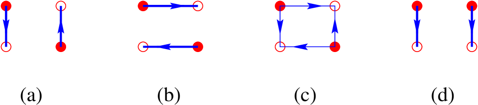
FIG. 1.: Locations of Dirac strings. (a), (b) each charge has one Dirac string. Two Dirac strings run in the opposite direction. (c) each charge has two Dirac strings. (d) each charge has one Dirac string. Two Dirac strings run in the same direction.

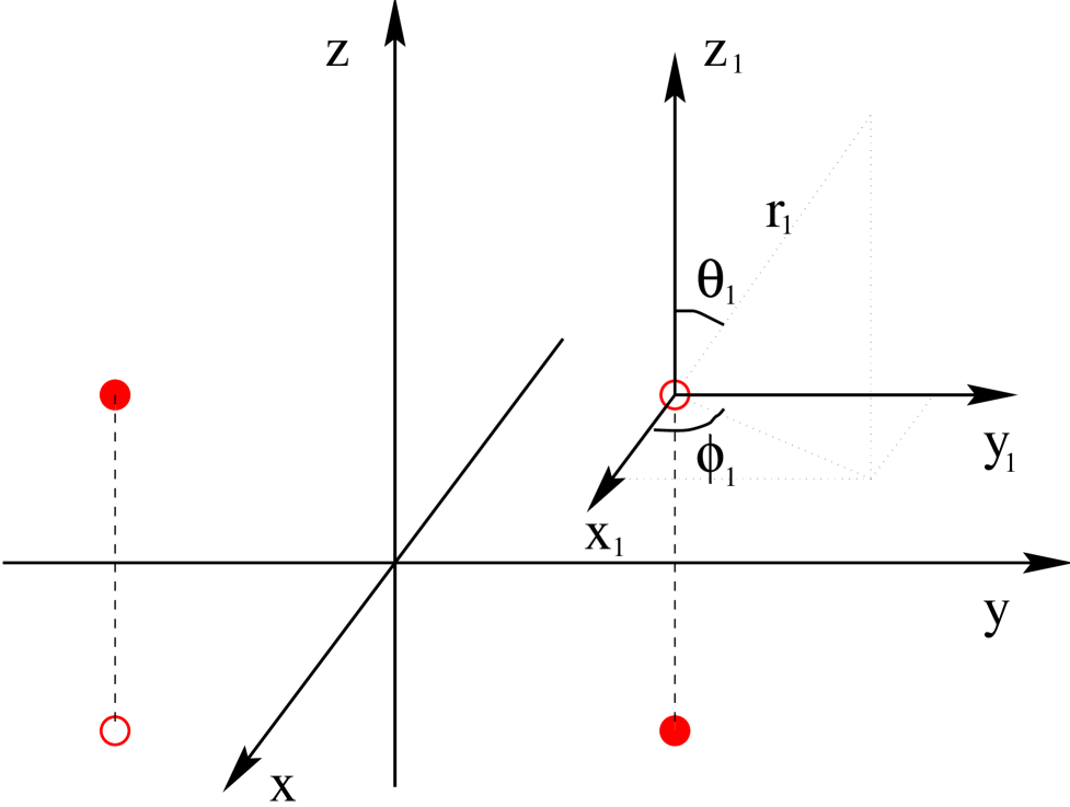
FIG. 2.: Coordinates used in Eq. (16).

FIG. 3.: Inter-quark potential derived from $SU(2)$ DGL theory when $e$=2.04, $\kappa=0.707$, $\sigma={(440\ \mbox{MeV})}^{2}$.

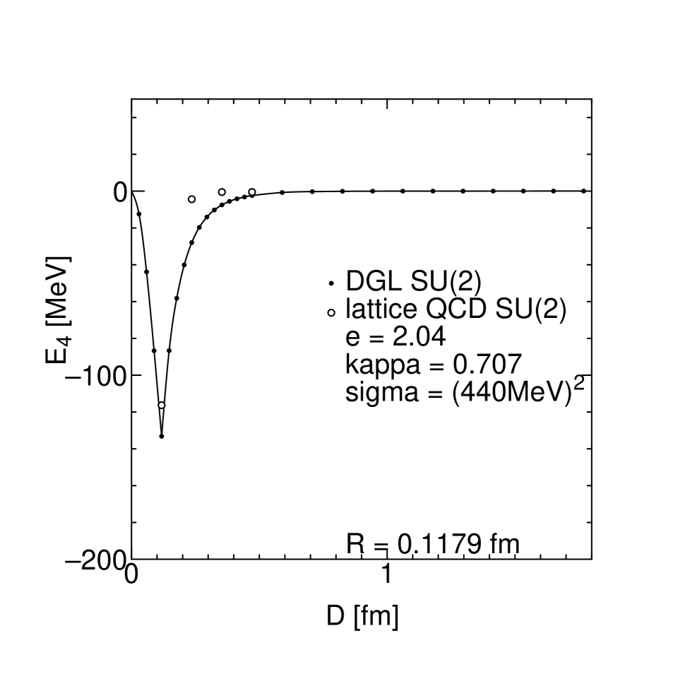
FIG. 4.: Inter-meson potential dreived from $SU(2)$ DGL theory (dot) when $e$=2.04, $\kappa$=0.707, $\sigma={(440\ \mbox{MeV})}^{2}$. The open circle denotes potential from $SU(2)$ lattice QCD in Ref. [14]. Quark charges are located at the corner of the rectangle and two Dirac strings run in the opposite direction (Figs. 1 (a) and (b)). $R$ is fixed to be $0.1179\ \mbox{fm}$.

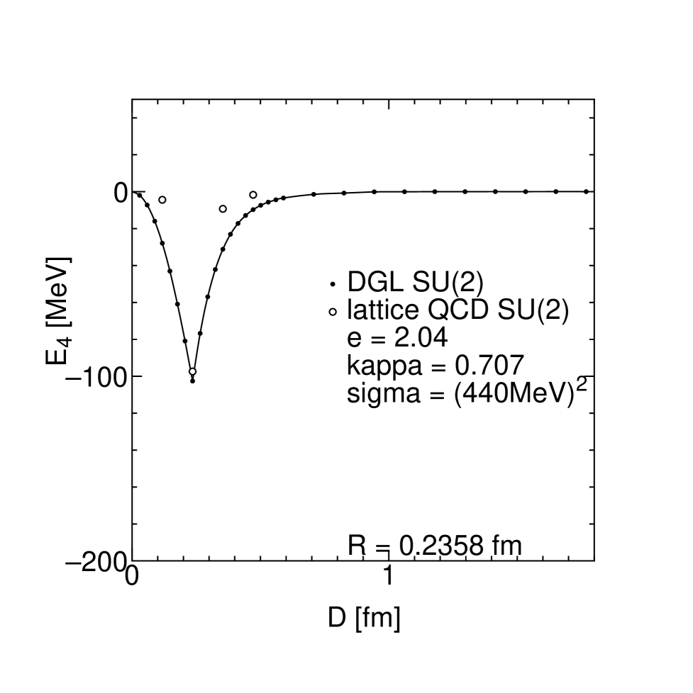
FIG. 5.: Inter-meson potential dreived from $SU(2)$ DGL theory when $R$ is fixed to be $0.2358\ \mbox{fm}$.

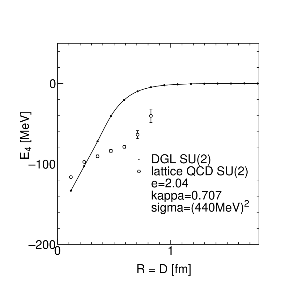
FIG. 6.: Inter-meson potential dreived from $SU(2)$ DGL theory in the $R=D$ case.

FIG. 7.: Inter-meson potential dreived from $SU(2)$ DGL theory when two Dirac srtings run in the same direction (Fig. 1 (d)). $R$ is fixed to be $0.1179\ \mbox{fm}$.

FIG. 8.: Color electric flux in confinement phase $v\neq 0$ (solid line) and that in Coulomb phase $v=0$ (dashed line). Color electric charges are located at $(x,y)$=($\pm$0.795 fm, $\pm$ 0.445 fm). Parameters are taken to be $e$=2.04, $\kappa$=0.707, $\sigma={(440\ \mbox{MeV})}^{2}$ .

REFERENCES

- [1] See, e.g., R. K. Bhaduri et al., Phys. Rev. Lett. 44 (1980), 1369 and refrence therein.
- [2] See, e.g., S. Matsuyama and H. Miyazawa, Prog. Theor. Phys. 61 (1978), 942.
- [3] See, e.g., F. Lenz et al., Ann. Phys. 170 (1986), 65 and reference therein.
- [4] T.Suzuki, Prog. Theor. Phys. 80 (1988), 929. S.Maedan and T.Suzuki, Prog. Theor. Phys. 81 (1989), 229.
- [5] G.’tHooft, in High Energy Physics, edited by A. Zichichi (Editorice Compositori, Bologna, 1975).
- [6] S. Mandelstam, Phys. Rep. 23C, (1976), 245.
- [7] G. ’tHooft, Nucl. Phys. B190 (1981), 455.
- [8] K. Bardacki and S. Samuel, Phys. Rev. D18 (1978), 2849.
- [9] D.Zwanziger, Phys. Rev. D3 (1971), 880.
- [10] S. Maedan et al., Prog. Theor. Phys. 84 (1990), 130.
- [11] S. Kamizawa et al., Nucl. Phys. B389 (1993), 563. T. Yazawa et.al, in preparation.
- [12] H. Monden et al., Phys. Lett. B294 (1992), 100.
- [13] Y. Matsubara, Review talk in ETC Workshop ’Nonperturbative Approaches to QCD’ (Trento 1995). H. Suganuma et.al., Nucl. Phys. B435 (1995), 207.
- [14] A. M. Green et al., Int. J. Mod. Phys. E2 (1993), 479.
- [15] T. Suzuki and I. Yotsuyanagi, Phys. Rev. D42 (1990), 4257. S. Hioki et al., Phys. Lett. B272 (1991), 326; errata, Phys. Lett. B281 (1992), 416, Nucl. Phys. B(Proc.Suppl.)30 (1992), 441.
- [16] J. S. Ball and A. Caticha, Phys. Rev. D11 (1975), 860.
- [17] V. Singh et al., LSU preprint LSUHEP-1-92(1992); Nucl. Phys. B(Proc.Suppl.)30 (1993), 568. P. Cea and L. Cosmai, Nucl. Phys. B(Proc.Suppl.)30 (1993), 572. Y. Matsubara et al., Nucl. Phys. B(Proc.Suppl.)30 (1993), 176.
- [18] H. Shiba and T. Suzuki, Phys. Lett. B351 (1995), 519. N. Arasaki et al., hep-lat/9608129.
- [19] J. Smit and A. J. van der Sijs, Nucl. Phys. B355 (1991), 603.