hep-ph/9704335 NIKHEF 97-018 VUTH 97-7 Modelling quark distribution and fragmentation functions

Abstract

The representation of quark distribution and fragmentation functions in terms of non-local operators is combined with a simple spectator model. This allows us to estimate these functions for the nucleon and the pion ensuring correct crossing and support properties. We give estimates for the unpolarized functions as well as for the polarized ones and for subleading (higher twist) functions. Furthermore we can study several relations that are consequences of Lorentz invariance and of C, P, and T invariance of the strong interactions.

I Introduction

Quark distribution functions and quark fragmentation functions appear in the field-theoretical description of hard processes as the parts that connect the quark and gluon lines to hadrons in the initial or final state. These parts are defined as connected matrix elements of non-local operators built from quark and gluon fields. The simplest, but most important ones, are the quark-quark correlation functions[1, 2, 3]. For each quark flavor one can write

$$\Phi_{ij}(p,P,S) = \int{d^{4}\xi\over(2\pi)^{4}}\ e^{-ip\cdot\xi}\ \langle P,S|\overline{\psi}_{j}(\xi)\psi_{i}(0)|P,S\rangle,$$ (1)

$$\Delta_{kl}(k,P_{h},S_{h}) = \sum_{X}\int{d^{4}\xi\over(2\pi)^{4}}\ e^{ik\cdot\xi}\ \langle 0|\psi_{k}(\xi)|P_{h},S_{h};X\rangle\ \langle P_{h},S_{h};X|\overline{\psi}_{l}(0)|0\rangle,$$ (2)

diagrammatically represented in Fig. 1.

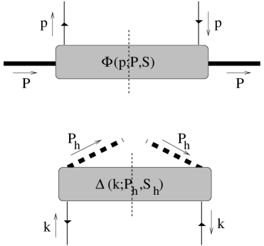
FIG. 1.: Diagrammatic representation of the correlation functions $\Phi$ and $\Delta$.

The hadron states are characterized by the momentum and spin vectors (limiting ourselves to spinless or spin 1/2 hadrons), $|P,S\rangle$ and $|P_{h},S_{h}\rangle$, for incoming and outgoing hadrons, respectively. The quark momenta are denoted $p$ and $k$, respectively. In the correlation function $\Delta$, the sum runs over all possible intermediate states that contain the hadron $h$ characterized by $P_{h}$ and $S_{h}$, while for $\Phi$ the sum is omitted assuming completeness. Furthermore a summation (average) over colors is understood in $\Phi$ ($\Delta$).

In a particular hard process only certain Dirac projections of the correlation functions appear and the non-locality is restricted by the integration over quark momenta. For inclusive lepton-hadron scattering, where the hard scale $Q$ is set by the spacelike momentum transfer $-q^{2}$ = $Q^{2}$, the correlation function $\Phi$ appears in the leading order result in an expansion in $1/Q$ of the cross section of hard processes. To be precise, the structure functions appearing in the cross sections can be expressed in terms of quark distribution functions, e.g., at leading order in $\alpha_{s}$, $2F_{1}(x_{\scriptscriptstyle B})$ = $F_{2}(x_{\scriptscriptstyle B})/x_{\scriptscriptstyle B}$ = $\sum_{a}e_{a}^{2}\,f_{1}^{a}(x_{\scriptscriptstyle B})$, where $x_{\scriptscriptstyle B}=Q^{2}/2P\cdot q$.

The unpolarized quark distribution function (omitting flavor index $a$) is obtained from $\Phi$ as

$$f_{1}(x) = \left.\frac{1}{2}\int dp^{-}\,d^{2}\mbox{\boldmath$p$}_{T}\ {\rm Tr}(\Phi\gamma^{+})\right|_{p^{+}=xP^{+}}$$ (3)

$$= \left.\int\frac{d\xi^{-}}{4\pi}\ e^{i\,p^{+}\xi^{-}}\langle P,S|\overline{\psi}(0)\gamma^{+}\psi(\xi)|P,S\rangle\right|_{\xi^{+}=\xi_{T}=0},$$ (4)

and depends only on the light-cone momentum fraction $x$ = $p^{+}/P^{+}$. The lightlike components $a^{\pm}\equiv a\cdot n_{\mp}$ are defined with the help of lightlike vectors $n_{\pm}$ satisfying $n_{+}^{2}$ = $n_{-}^{2}$ = 0 and $n_{+}\cdot n_{-}$ = 1. In inclusive lepton-hadron scattering they are related to the hadron momentum $P$ and the hard momentum $q$ as

$$P = {M^{2}x_{b}\over Q\sqrt{2}}\ n_{-}+{Q\over x_{b}\sqrt{2}}\ n_{+},$$ (5)

$$q = {Q\over\sqrt{2}}\ n_{-}-{Q\over\sqrt{2}}\ n_{+},$$ (6)

where $M$ is the mass of the hadron. The non-locality is restricted to a lightlike separation. At this point it should be noted that there are other contributions in the leading cross section resulting from soft parts with $A^{+}$ gluon legs. These can be absorbed into the correlation function providing the link operator that renders the definition in Eqs. (1) and (2) color gauge invariant. Choosing the $A^{+}=0$ gauge in the study of $\Phi$ the link operator reduces to unity.

The simplest example of a hard process in which the correlation function $\Delta$ appears is 1-particle inclusive $e^{+}e^{-}$ annihilation. In that case the scale is set by the momentum squared of the annihilating leptons, $q^{2}$ = $Q^{2}$ and the production cross section in leading order becomes proportional to fragmentation functions $D_{1}^{a\rightarrow h}(z_{h})$, where $z_{h}$ = $2P_{h}\cdot q/q^{2}$. The quark fragmentation function (omitting flavor index $a$) is obtained from $\Delta$ as

$$D_{1}(z) = \left.\frac{1}{4z}\int dk^{+}\,d^{2}\mbox{\boldmath$k$}_{T}\ {\rm Tr}(\Delta\gamma^{-})\right|_{k^{-}=P_{h}^{-}/z}$$ (7)

$$= \left.\int\frac{d\xi^{+}}{8\pi\,z}\ e^{i\,k^{-}\xi^{+}}\ {\rm Tr}\left(\gamma^{-}\langle 0|\psi(\xi)|P_{h},S_{h};X\rangle\langle P_{h},S_{h};X|\overline{\psi}(0)|0\rangle\right)\right|_{\xi^{-}=\xi_{T}=0},$$ (8)

and depends only on the light-cone momentum fraction $z$ = $P_{h}^{-}/k^{-}$. Taking as an explicit example 1-particle inclusive electron-positron annihilation, the lightlike vectors are defined from the hadron momentum $P_{h}$ and the hard momentum $q$:

$$P_{h} = {z_{h}Q\over\sqrt{2}}\ n_{-}+{M_{h}^{2}\over z_{h}Q\sqrt{2}}\ n_{+},$$ (9)

$$q = {Q\over\sqrt{2}}\ n_{-}+{Q\over\sqrt{2}}\ n_{+},$$ (10)

where $M_{h}$ is the mass of the produced hadron. The non-locality in the expression for $D_{1}$ is again restricted to a lightlike separation. The link operator needed for color gauge invariance becomes invisible by using the gauge $A^{-}$ = 0 in the study of $\Delta$.

As soon as in a hard process two hadrons (or for that matter one jet and one hadron) play a role, the transverse directions become important. Examples are inclusive Drell-Yan scattering, 1-particle inclusive lepton-hadron scattering or 2-particle inclusive $e^{+}e^{-}$ annihilation. For instance, in inclusive lepton-hadron scattering the leading order cross section is given by the handbag diagram containing only one soft part $\Phi$, shown in Fig. 1, but in 1-particle inclusive lepton-hadron scattering the leading order cross section involves also the fragmentation of the quark, the part $\Delta$ in Fig. 1. In order to describe the current fragmentation one can still define lightlike vectors $n_{\pm}$ using the hadronic momenta as in Eqs. (5) and (9), but the third momentum, in casu the hard momentum $q$, contains a transverse piece. Up to $M^{2}/Q^{2}$ corrections (irrelevant for our purposes), $P$ is proportional to $n_{+}$, $P_{h}$ is proportional to $n_{-}$ and

$$q={Q\over\sqrt{2}}\ n_{-}-{Q\over\sqrt{2}}\ n_{+}+q_{T}.$$ (11)

By selecting observables depending on the transverse momentum scale $-q_{T}^{2}$ = $Q_{T}^{2}\ll Q^{2}$ one needs to consider distribution functions and fragmentation functions before integrating over $\mbox{\boldmath$p$}_{T}$ or $\mbox{\boldmath$k$}_{T}$, respectively. Examples are the dependence on the transverse momentum of the produced lepton pair in Drell-Yan scattering, the dependence on the transverse momentum of a produced hadron belonging to the current jet in lepton-hadron scattering or the transverse momentum distribution of hadrons with respect to the jet-axis (or with respect to a fast hadron in the opposite jet) in the case of back-to-back jets in $e^{+}e^{-}$ annihilation.

In this paper, we review the structure of light-cone correlation functions including the effects of transverse separation of the quark fields, and we estimate them using a simple model. This will be done for all possible Dirac projections that contribute in leading or subleading order. Thus we obtain estimates not only for the usual unpolarized distribution and fragmentation functions, but also for the polarized ones and for subleading (higher twist) functions. As we will see, in a number of cases there are relations between leading and subleading $\mbox{\boldmath$p$}_{T}$-integrated functions.

Although hard cross sections can be expressed in terms of distribution and fragmentation functions, these objects cannot be calculated from QCD because they involve the hadronic bound states (at least not for light quarks). Even the simplest case, the moments that are related to matrix elements of local operators require non-perturbative methods like, for instance, lattice calculations. The full ($x$-dependent) quark distribution, however, requires the knowledge of all moments. We follow here a different route. We want to investigate the structure of light-cone correlation functions and illustrate the consequences of various constraints in a simple model. Particularly suitable is a model in which the spectrum of intermediate states, which can be inserted in Eq. (1) or is explicitly present in Eq. (2), is replaced by one state, referred to as a diquark, if the hadron is a baryon. At that point one still has lots of freedom to parametrize the hadron-quark-diquark vertex. We make the ansatz that in the zero-binding limit implies the simple symmetric $SU(6)$ spin-flavor structure. As parameters to describe the vertex one then has only the quark mass, a diquark mass and a size parameter left.

Although there are a few parameters, the approach has the advantage of being covariant and producing the right support, in contrast to the use of other models [4], such as bag models [5, 6, 7], quark models [8, 9, 10] or soliton models [11, 12, 13], which require projection techniques [14]. Of course, these models have the advantage that they also reproduce other observables. Similar spectator models have also been used for the calculation of distributions [15, 16] and fragmentation functions [17].

Of course, matrix elements as discussed above have a scale dependence, which in expressions for hard cross sections shows up as a logarithmic dependence on the hard scale. A well known problem is that the modelling does not provide a scale dependence. Models with a simple valence quark input, as we take as our starting point, will be naturally ‘low scale models’. In principle, this could be evolved to higher scales to allow comparison with data. However, we lack evolution equations at low scales. On the other hand, we also consider higher twist distributions, for which evolution is much more involved than the twist two case [18]. These are the reasons for not including evolution in this paper. In other words, radiative corrections and their absorption in the scale dependence of the quark distributions are not taken into account.

The setup of the paper is the following. In section II we discuss the structure of light-cone correlation functions, both quark distribution functions and quark fragmentation functions. In section III we present the diquark spectator approach and the construction of the vertices. The results for the distribution and fragmentation functions are given in section IV. We end with a summary and outlook.

II Quark correlation functions

A Distribution functions

In order to study the correlation function $\Phi$ it is useful to realize that its form is constrained by the hermiticity properties of the fields and invariance under parity operation. The most general expression for $\Phi$ consistent with these constraints is [19, 20]:

$$\Phi(p,P,S) = M\,A_{1}+A_{2}\,\hbox to0.0pt{\hbox to7.80904pt{\hfil/\hfil}\hss}P+A_{3}\,\hbox to0.0pt{\hbox to5.03125pt{\hfil/\hfil}\hss}p+{A_{4}\over M}\,\sigma^{\mu\nu}P_{\mu}p_{\nu}+i\ A_{5}\,p\cdot S\ \gamma_{5}+M\,A_{6}\,\hbox to0.0pt{\hbox to6.70831pt{\hfil/\hfil}\hss}S\,\gamma_{5}$$ (14)

$$+{A_{7}\over M}\,p\cdot S\ \hbox to0.0pt{\hbox to7.80904pt{\hfil/\hfil}\hss}P\,\gamma_{5}+{A_{8}\over M}\,p\cdot S\ \hbox to0.0pt{\hbox to5.03125pt{\hfil/\hfil}\hss}p\,\gamma_{5}+i\,A_{9}\,\sigma^{\mu\nu}\,\gamma_{5}\ S_{\mu}P_{\nu}$$

$$+i\,A_{10}\,\sigma^{\mu\nu}\,\gamma_{5}\,S_{\mu}p_{\nu}+i\,{A_{11}\over M^{2}}\,p\cdot S\ \sigma^{\mu\nu}\,\gamma_{5}\,p_{\mu}P_{\nu}+{A_{12}\over M}\,\epsilon_{\mu\nu\rho\sigma}\,\gamma^{\mu}P^{\nu}p^{\rho}S^{\sigma},$$

where the amplitudes $A_{i}$ depend on $\sigma\equiv 2p\cdot P$ and $\tau\equiv p^{2}$. Hermiticity requires all amplitudes $A_{i}(\sigma,\tau)$ to be real. Time reversal invariance can also be used and requires the amplitudes $A_{4}$, $A_{5}$ and $A_{12}$ to be purely imaginary, hence they vanish.

In hard processes the hard momentum scale $q$ and the hadron momentum $P$ define the lightlike directions $n_{\pm}$. The momentum $P$ is parametrized as in Eq. (5). The spin vector $S$ and the quark momentum $p$ are also expanded in the lightlike vectors and transverse components:

$$p={x_{\scriptscriptstyle B}(p^{2}+{\mbox{\boldmath$p$}}_{T}^{2})\over xQ\sqrt{2}}\ n_{-}+{xQ\over x_{\scriptscriptstyle B}\sqrt{2}}\ n_{+}+p_{T},$$ (15)

$$S=-{\lambda Mx_{\scriptscriptstyle B}\over Q\sqrt{2}}\ n_{-}+{\lambda Q\over Mx_{\scriptscriptstyle B}\sqrt{2}}\ n_{+}+S_{T}.$$ (16)

Thus $x$ represents the fraction of the momentum in the $+$ direction carried by the quark inside the hadron. In the transverse space the following projectors can be used

$$g_{T}^{\mu\nu}=g^{\mu\nu}-n_{+}^{\{\mu}n_{-}^{\nu\}},$$ (17)

$$\epsilon_{T}^{\mu\nu}=\epsilon^{-+\mu\nu}.$$ (18)

Considering a hard scattering process up to order $1/Q^{2}$, the component of $p$ along $n_{-}$ is irrelevant and one encounters the quantities

$$\Phi^{[\Gamma]}\left(x,{\mbox{\boldmath$p$}}_{T}\right)=\left.{1\over 2}\int dp^{-}\ {\rm Tr}\left(\Phi\Gamma\right)\right|_{p^{+}=xP^{+},p_{T}}=\int[d\sigma d\tau\,\delta(\ )]\ \frac{{\rm Tr}(\Phi\Gamma)}{4P^{+}},$$ (19)

where we used the shorthand notation

$$\left[d\sigma d\tau\,\delta(\ )\right]=d\sigma d\tau\ \delta\left(\tau-x\sigma+x^{2}M^{2}+{\mbox{\boldmath$p$}}_{T}^{2}\right).$$ (20)

The projections of $\Phi$ on different Dirac structures define distribution functions. They are related to integrals over linear combinations of the amplitudes. The projections

$$\Phi^{[\gamma^{+}]}(x,{\mbox{\boldmath$p$}}_{T}) \equiv f_{1}(x,{\mbox{\boldmath$p$}}_{T}^{2})$$ (21)

$$= \int[d\sigma d\tau\,\delta(\ )]\left[A_{2}+xA_{3}\right],$$ (22)

$$\Phi^{[\gamma^{+}\gamma_{5}]}(x,{\mbox{\boldmath$p$}}_{T}) \equiv \lambda g_{1L}(x,{\mbox{\boldmath$p$}}_{T}^{2})+\frac{\,{\mbox{\boldmath$p$}}_{T}\!\cdot\!{\mbox{\boldmath$S$}}_{T}\,}{M}g_{1T}(x,{\mbox{\boldmath$p$}}_{T}^{2})$$ (24)

$$= \int[d\sigma d\tau\,\delta(\ )]\Biggl{\{}\lambda\left[-A_{6}-\left(\frac{\sigma-2x\,M^{2}}{2M^{2}}\right)\;\left(A_{7}+xA_{8}\right)\right]+\frac{\,{\mbox{\boldmath$p$}}_{T}\!\cdot\!{\mbox{\boldmath$S$}}_{T}\,}{M}\;\left(A_{7}+xA_{8}\right)\Biggr{\}},$$ (25)

$$\Phi^{[i\sigma^{i+}\gamma_{5}]}(x,{\mbox{\boldmath$p$}}_{T}) \equiv S_{T}^{i}h_{1T}(x,{\mbox{\boldmath$p$}}_{T}^{2})+\frac{p_{T}^{i}}{M}\left(\lambda h_{1L}^{\perp}(x,{\mbox{\boldmath$p$}}_{T}^{2})+\frac{\,{\mbox{\boldmath$p$}}_{T}\!\cdot\!{\mbox{\boldmath$S$}}_{T}\,}{M}h_{1T}^{\perp}(x,{\mbox{\boldmath$p$}}_{T}^{2})\right)$$ (27)

$$= \int[d\sigma d\tau\,\delta(\ )]\Biggl{\{}-S_{T}^{i}(A_{9}+xA_{10})+\frac{\lambda\,p_{T}^{i}}{M}\left[A_{10}-\left(\frac{\sigma-2x\,M^{2}}{2M^{2}}\right)\;A_{11}\right]$$ (29)

$$\qquad\qquad\qquad\mbox{}+\frac{p_{T}^{i}}{M}\;\frac{\,{\mbox{\boldmath$p$}}_{T}\!\cdot\!{\mbox{\boldmath$S$}}_{T}\,}{M}\;A_{11}\Biggr{\}},$$

are leading in $1/Q$. For the distribution functions, this is indicated by the subscript $1$ in the names of the functions [21]. The following projections occur with a pre-factor $M/P^{+}$, which signals the subleading (or higher twist) nature of the corresponding distribution functions

$$\Phi^{[1]}(x,{\mbox{\boldmath$p$}}_{T}) \equiv \frac{M}{P^{+}}\,e(x,{\mbox{\boldmath$p$}}_{T}^{2})$$ (30)

$$= \frac{M}{P^{+}}\int[d\sigma d\tau\,\delta(\ )]\ A_{1},$$ (31)

$$\Phi^{[\gamma^{i}]}(x,{\mbox{\boldmath$p$}}_{T}) \equiv \frac{p_{T}^{i}}{P^{+}}\,f^{\perp}(x,{\mbox{\boldmath$p$}}_{T}^{2})$$ (33)

$$= \frac{M}{P^{+}}\int[d\sigma d\tau\,\delta(\ )]\frac{p_{T}^{i}}{M}\;A_{3},$$ (34)

$$\Phi^{[\gamma^{i}\gamma_{5}]}(x,{\mbox{\boldmath$p$}}_{T}) \equiv \frac{M\,S_{T}^{i}}{P^{+}}\,g^{\prime}_{T}(x,{\mbox{\boldmath$p$}}_{T}^{2})+\frac{p_{T}^{i}}{P^{+}}\left(\lambda g_{L}^{\perp}(x,{\mbox{\boldmath$p$}}_{T}^{2})+\frac{\,{\mbox{\boldmath$p$}}_{T}\!\cdot\!{\mbox{\boldmath$S$}}_{T}\,}{M}g_{T}^{\perp}(x,{\mbox{\boldmath$p$}}_{T}^{2})\right)$$ (36)

$$= \frac{M}{P^{+}}\int[d\sigma d\tau\,\delta(\ )]\left\{-S_{T}^{i}\;A_{6}-\frac{\lambda\,p_{T}^{i}}{M}\,\left(\frac{\sigma-2x\,M^{2}}{2M^{2}}\right)\;A_{8}+\frac{p_{T}^{i}}{M}\,\frac{\,{\mbox{\boldmath$p$}}_{T}\!\cdot\!{\mbox{\boldmath$S$}}_{T}\,}{M}\;A_{8}\right\},$$ (37)

$$\Phi^{[i\sigma^{ij}\gamma_{5}]}(x,{\mbox{\boldmath$p$}}_{T}) \equiv \frac{S_{T}^{i}p_{T}^{j}-S_{T}^{j}p_{T}^{i}}{P^{+}}\,h_{T}^{\perp}(x,{\mbox{\boldmath$p$}}_{T}^{2})$$ (39)

$$= \frac{M}{P^{+}}\int[d\sigma d\tau\,\delta(\ )]\frac{S_{T}^{i}p_{T}^{j}-S_{T}^{j}p_{T}^{i}}{M}\;\left[-A_{10}\right],$$ (40)

$$\Phi^{[i\sigma^{+-}]}(x,{\mbox{\boldmath$p$}}_{T}) \equiv \frac{M}{P^{+}}\left(\lambda h_{L}(x,{\mbox{\boldmath$p$}}_{T}^{2})+\frac{\,{\mbox{\boldmath$p$}}_{T}\!\cdot\!{\mbox{\boldmath$S$}}_{T}\,}{M}\,h_{T}(x,{\mbox{\boldmath$p$}}_{T}^{2})\right)$$ (42)

$$= \frac{M}{P^{+}}\int[d\sigma d\tau\,\delta(\ )]\Biggl{\{}\lambda\,\Biggl{[}-A_{9}-\frac{\sigma}{2M^{2}}\,A_{10}+\left(\frac{\sigma-2x\,M^{2}}{2M^{2}}\right)^{2}\,A_{11}\Biggr{]}$$ (44)

$$\qquad\qquad\qquad\mbox{}-\frac{\,{\mbox{\boldmath$p$}}_{T}\!\cdot\!{\mbox{\boldmath$S$}}_{T}\,}{M}\,\left(\frac{\sigma-2x\,M^{2}}{2M^{2}}\right)\,A_{11}\Biggr{\}}.$$

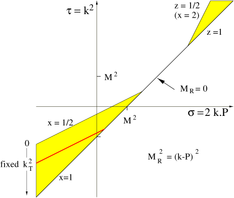
FIG. 2.: The $\delta$-function constraint in the $\sigma$-$\tau$ plane (using quark momentum $k$ and hadron momentum $P$) coming from fixing $x$ and $\mbox{\boldmath$k$}_{T}^{2}$ in the expression for the distribution functions $F(x,\mbox{\boldmath$k$}_{T}^{2})$ (and similarly for the fragmentation functions $D(z,z^{2}\mbox{\boldmath$k$}_{T}^{2})$) and the full integration regions for the $\mbox{\boldmath$k$}_{T}$ integrated functions $F(x)$ (and similarly for $D(z)$). The latter region is determined by $\mbox{\boldmath$k$}_{T}^{2}\geq 0$ and $M_{R}^{2}\geq 0$.

The constraint of the $\delta$-function in the integration over $\sigma$ and $\tau$ is indicated in Fig. 2. Furthermore, the integration is restricted to the region $M_{R}^{2}\equiv(P-p)^{2}\geq 0$. This leads to the vanishing of the distribution functions at $x=1$.

If a generic distribution function is written as

$$F(x,{\mbox{\boldmath$p$}}_{T}^{2})=\int[d\sigma d\tau\,\delta(\ )]\ G\left(A_{i}(\sigma,\tau),\sigma,x\right),$$ (45)

symmetric integration over ${\mbox{\boldmath$p$}}_{T}$ gives

$$F(x)=\int[d\sigma d\tau\theta(\ )]\ G\left(A_{i}(\sigma,\tau),\sigma,x\right),$$ (46)

where

$$[d\sigma d\tau\,\theta(\ )]=d\sigma d\tau\ \theta\left(x\sigma-x^{2}M^{2}-\tau\right).$$ (47)

The region covered by the $\theta$-function (for $x=1/2$) is the lower shaded region in Fig. 2 corresponding to ${\mbox{\boldmath$p$}}_{T}^{2}\geq 0$. Only the terms involving the distribution functions $f_{1}$, $g_{1}=g_{1L}$, $h_{1}=h_{1T}+({\mbox{\boldmath$p$}}_{T}^{2}/2M^{2})\,h_{1T}^{\perp}$, $e$, $g_{T}=g^{\prime}_{T}+({\mbox{\boldmath$p$}}_{T}^{2}/2M^{2})\,g_{T}^{\perp}$ and $h_{L}$ are non-vanishing upon integration over ${\mbox{\boldmath$p$}}_{T}$. The integrated functions $f_{1}(x)$, $g_{1}(x)$ and $h_{1}(x)$ have the well known probabilistic interpretations. $f_{1}(x)$ gives the probability of finding a quark with light-cone momentum fraction $x$ in the $+$ direction (and any transverse momentum). $g_{1}(x)$ is a chirality distribution: in a hadron that is in a positive helicity eigenstate ($\lambda=1$), it measures the probability of finding a right-handed quark with light-cone momentum fraction $x$ minus the the probability of finding a left-handed quark with the same light-cone momentum fraction (and any transverse momentum). $h_{1}(x)$ is a transverse spin distribution: in a transversely polarized hadron, it measures the probability of finding quarks with light-cone momentum fraction $x$ polarized along the direction of the polarization of the hadron minus the probability of finding quarks with the same light-cone momentum fraction polarized along the direction opposite to the polarization of the hadron. The twist three functions have no intuitive partonic interpretation. Nevertheless, they are well defined as hadronic matrix elements via Eqs. (1) and (2), and their projections.

We note the appearance of higher $\mbox{\boldmath$p$}_{T}^{2}$-moments,

$$F^{(n)}(x) \equiv \int d^{2}{\mbox{\boldmath$p$}}_{T}\ \left({{\mbox{\boldmath$p$}}_{T}^{2}\over 2M^{2}}\right)^{n}F(x,{\mbox{\boldmath$p$}}_{T}^{2})$$ (48)

$$= \pi\int[d\sigma d\tau\,\theta(\ )]\ \left(\frac{x\sigma-x^{2}M^{2}-\tau}{2M^{2}}\right)^{n}\ G\left(A_{i}(\sigma,\tau),\sigma,x\right),$$ (49)

such as $h_{1T}^{\perp(1)}$ and $g_{T}^{\perp(1)}$. The equality in Eq. (49) is obtained using the azimuthal symmetry of the distribution functions, which depend only on $x$ and ${\mbox{\boldmath$p$}}_{T}^{2}$. In the weighted integration, $\int d^{2}\mbox{\boldmath$p$}_{T}\,p_{T}^{i}\ldots$ one will encounter the functions $g_{1T}^{(1)}$ and $h_{1L}^{\perp(1)}$.

The distribution functions cannot be all independent because their number is larger than the number of amplitudes $A_{i}$. This is reflected in relations such as

$$g_{T}(x) = g_{1}(x)+{d\over dx}\ g_{1T}^{(1)}(x),$$ (50)

$$h_{L}(x) = h_{1}(x)-{d\over dx}\ h_{1L}^{\perp(1)}(x),$$ (51)

$$h_{T}^{(1)}(x) = -\frac{1}{2}\,\frac{d}{dx}\ h_{1T}^{\perp(2)}(x),$$ (52)

which can be obtained using their explicit expressions in terms of the amplitudes.

The functions $g_{2}=g_{T}-g_{1}$ and $h_{2}=2(h_{L}-h_{1})$ thus satisfy the sum rules

$$\int_{0}^{1}dx\ g_{2}(x) = -g_{1T}^{(1)}(0),$$ (53)

$$\int_{0}^{1}dx\ h_{2}(x) = 2\,h_{1L}^{\perp(1)}(0),$$ (54)

which are a direct consequence of (50) and (51). If the functions $g_{1T}^{(1)}$ and $h_{1L}^{\perp(1)}$ vanish at the origin, we rediscover the Burkhardt-Cottingham sum rule [22] and the Burkardt sum rule [23]. These sum rules (Eqs. (53) and (54) with vanishing right-hand sides) can also be derived using Lorentz covariance for the expectation values of local operators [24]. In our approach this would imply constraints on the amplitudes $A_{i}$.

B Fragmentation functions

The correlation function $\Delta$ is also constrained by the hermiticity properties of the fields and invariance under parity operation, leading to an expansion identical to that in Eq. (14) with the replacements $\left\{p,P,S,M\right\}\to\left\{k,P_{h},S_{h},M_{h}\right\}$ [21] and with real amplitudes, say $B_{i}$, now depending on $\tau_{h}\equiv k^{2}$ and $\sigma_{h}\equiv 2k\cdot P_{h}$. Time reversal invariance does not imply any constraints on the amplitudes, thus $B_{4}$, $B_{5}$ and $B_{12}$, referred to as ‘T-odd’, are, in general, non-vanishing. (For a discussion on T-odd fragmentation functions, see [25]).

In hard processes one encounters the quantities

$$\Delta^{[\Gamma]}\left(z,{\mbox{\boldmath$k$}}_{T}\right)=\left.{1\over 4z}\ \int dk^{+}\ {\rm Tr}\left(\Delta\Gamma\right)\right|_{k^{-}=P_{h}^{-}/z,k_{T}}=\int\left[d\sigma_{h}d\tau_{h}\,\delta(\ )\right]\ \frac{{\rm Tr}(\Delta\Gamma)}{8z\,P_{h}^{-}},$$ (55)

where we used the shorthand notation

$$\left[d\sigma_{h}d\tau_{h}\,\delta(\ )\right]=d\sigma_{h}d\tau_{h}\ \delta\left(\tau_{h}-\frac{\sigma_{h}}{z}+\frac{M_{h}^{2}}{z^{2}}+{\mbox{\boldmath$k$}}_{T}^{2}\right).$$ (56)

The momentum $P_{h}$ is parametrized as in Eq. (9) and is used to define the lightlike vectors, in terms of which the vectors $S_{h}$ and $k$ can also expanded:

$$k={z_{h}Q\over z\sqrt{2}}\ n_{-}+{z(k^{2}+{\mbox{\boldmath$k$}}_{T}^{2})\over z_{h}Q\sqrt{2}}\ n_{+}+k_{T},$$ (57)

$$S_{h}={\lambda_{h}z_{h}Q\over M_{h}\sqrt{2}}\ n_{-}-{\lambda_{h}M_{h}\over z_{h}Q\sqrt{2}}\ n_{+}+S_{hT}.$$ (58)

Thus $z$ is the fraction of the momentum in the $-$ direction carried by the hadron $h$ originating from the fragmentation of the quark. The spin vector satisfies $P_{h}\cdot S_{h}$ = 0 and for a pure state $-S_{h}^{2}$ = $\lambda_{h}^{2}+\mbox{\boldmath$S$}_{hT}^{2}$ = 1.

Comparing the above equations with the case of the distribution functions, one sees that the relations between the Dirac projections $2z\,\Delta^{[\Gamma]}(z,\mbox{\boldmath$k$}_{T})$ and the amplitudes are identical to those for $\Phi^{[\Gamma]}(x,\mbox{\boldmath$p$}_{T})$ after the replacements $\left\{x,\sigma,\tau,{\mbox{\boldmath$p$}}_{T},P,S_{T},\lambda,M,A_{i},\pm-\mbox{components}\right\}\to\left\{1/z,\sigma_{h},\tau_{h},{\mbox{\boldmath$k$}}_{T},P_{h},S_{hT},\lambda_{h},M_{h},B_{i},\mp-\mbox{components}\right\}$, except for additional parts originating from the T-odd functions. Furthermore, the definition of fragmentation functions follow the general procedure used to define distribution functions. We use for the names of the fragmentation functions capital letters (with the only exception for the counterparts of $f_{..}$ functions which are called $D_{..}$). For example,

$$\Delta^{[\gamma^{-}]}(z,{\mbox{\boldmath$k$}}_{T}) \equiv D_{1}(z,\mbox{\boldmath$k$}_{T}^{\prime 2})+\frac{\epsilon_{T}^{ij}k_{Ti}S_{hTj}}{M_{h}}D_{1T}^{\perp}(z,\mbox{\boldmath$k$}_{T}^{\prime 2})$$ (59)

$$= \frac{1}{2z}\int[d\sigma_{h}d\tau_{h}\,\delta(\ )]\Biggl{\{}\left[B_{2}+\frac{1}{z}\,B_{3}\right]+\frac{\epsilon_{T}^{ij}k_{Ti}S_{hTj}}{M_{h}}\,B_{12}\Biggr{\}},$$ (60)

where ${\mbox{\boldmath$k$}}^{\prime}_{T}=-z{\mbox{\boldmath$k$}}_{T}$. The choice of arguments $z$ and ${\mbox{\boldmath$k$}}^{\prime}_{T}$ in the fragmentation functions is worth a comment. In the expansion of $k$ in Eq. (57) the quantities $1/z$ and ${\mbox{\boldmath$k$}}_{T}$ appear in a natural way. However, in the interpretation of $\Delta$ as a decay function of quarks, the variable $z$ as the ratio of $P_{h}^{-}/k^{-}$ is more adequate. Applying a Lorentz transformation that leaves the $-$ component (and hence the definition of $z$) unchanged, one finds that ${\mbox{\boldmath$k$}}^{\prime}_{T}=-z{\mbox{\boldmath$k$}}_{T}$ is the transverse component of hadron $h$ with respect to the quark momentum.

Further, we only display the additional parts of projections which come from the time reversal odd amplitudes and which, thus, have no counterparts in the distribution functions. In the leading twist projections there is only one other projection with an additional term,

$$\Delta^{[i\sigma^{i-}\gamma_{5}]}(z,{\mbox{\boldmath$k$}}_{T}) \equiv \ldots+\frac{\epsilon_{T}^{ij}k_{Tj}}{M_{h}}H_{1}^{\perp}(z,{\mbox{\boldmath$k$}}_{T}^{\prime 2})$$ (61)

$$= \ldots+\frac{1}{2z}\int[d\sigma_{h}d\tau_{h}\,\delta(\ )]\,\frac{\epsilon_{T}^{ij}k_{Tj}}{M_{h}}\left[-B_{4}\right].$$ (62)

At subleading twist there are five additional T-odd structures:

$$\Delta^{[\gamma^{i}]}(z,{\mbox{\boldmath$k$}}_{T}) \equiv \ldots+\frac{M_{h}}{P_{h}^{-}}\left(\lambda_{h}\frac{\epsilon_{T}^{ij}k_{Tj}}{M_{h}}D_{L}^{\perp}(z,{\mbox{\boldmath$k$}}_{T}^{\prime 2})+\epsilon_{T}^{ij}S_{hTj}D_{T}(z,{\mbox{\boldmath$k$}}_{T}^{\prime 2})\right)$$ (63)

$$= \ldots+\frac{M_{h}}{2zP_{h}^{-}}\int[d\sigma_{h}d\tau_{h}\,\delta(\ )]\left\{-\lambda_{h}\frac{\epsilon_{T}^{ij}k_{Tj}}{M_{h}}\,B_{12}-\epsilon_{T}^{ij}S_{hTj}\left(\frac{\sigma_{h}-2M_{h}^{2}/z}{2M_{h}^{2}}\right)B_{12}\right\},$$ (64)

$$\Delta^{[i\gamma_{5}]}(z,{\mbox{\boldmath$k$}}_{T}) \equiv \ldots+\frac{M_{h}}{P_{h}^{-}}\left(\lambda_{h}E_{L}(z,{\mbox{\boldmath$k$}}_{T}^{\prime 2})+\frac{\,{\mbox{\boldmath$k$}}_{T}\!\cdot\!{\mbox{\boldmath$S$}}_{hT}\,}{M_{h}}E_{T}(z,{\mbox{\boldmath$k$}}_{T}^{\prime 2})\right)$$ (66)

$$= \ldots+\frac{M_{h}}{2zP_{h}^{-}}\int[d\sigma_{h}d\tau_{h}\,\delta(\ )]\left\{-\lambda_{h}\left(\frac{\sigma_{h}-2M_{h}^{2}/z}{2M_{h}^{2}}\right)\,B_{5}+\frac{\,{\mbox{\boldmath$k$}}_{T}\!\cdot\!{\mbox{\boldmath$S$}}_{hT}\,}{M_{h}}\,B_{5}\right\},$$ (67)

$$\Delta^{[i\sigma^{ij}\gamma_{5}]}(z,{\mbox{\boldmath$k$}}_{T}) \equiv \ldots+\frac{M_{h}}{P_{h}^{-}}\epsilon_{T}^{ij}H(z,{\mbox{\boldmath$k$}}_{T}^{\prime 2})$$ (69)

$$= \ldots+\frac{M_{h}}{2zP_{h}^{-}}\int[d\sigma_{h}d\tau_{h}\,\delta(\ )]\left\{\epsilon_{T}^{ij}\left(\frac{\sigma_{h}-2M_{h}^{2}/z}{2M_{h}^{2}}\right)\,B_{4}\right\}.$$ (70)

The constraint imposed by the $\delta$-function in the $\sigma_{h}$-$\tau_{h}$ plane is also indicated in Fig. 2. The integration is restricted to the region $M_{R}^{2}=(P_{h}-k)^{2}\geq 0$, which implies that the fragmentation functions vanish at $z=1$. We note the reciprocity of $x$ and $z$, i.e., the constraint for $z=1/2$ is the same as one would have for $x$ = 2. Note, however, that the integration involves different regions. For the distributions one has (roughly) spacelike quark momenta, for the fragmentation timelike quark momenta. If a generic quark fragmentation function is given by

$$D(z,{{\mbox{\boldmath$k$}}^{\prime}_{T}}^{2})={1\over 2z}\int[d\sigma_{h}d\tau_{h}\,\delta(\ )]\ G(B_{i}(\sigma_{h},\tau_{h}),\sigma_{h},z),$$ (71)

the integrated functions are given by

$$D^{(n)}(z) \equiv z^{2}\int d^{2}{\mbox{\boldmath$k$}}_{T}\left({{\mbox{\boldmath$k$}}_{T}^{2}\over 2M_{h}^{2}}\right)^{n}D(z,{\mbox{\boldmath$k$}}_{T}^{2})$$ (72)

$$= \frac{\pi\,z}{2}\int[d\sigma_{h}d\tau_{h}\,\theta(\ )]\left(\frac{\sigma_{h}-2M_{h}^{2}/z}{2M_{h}^{2}}\right)^{n}G(B_{i}(\sigma_{h},\tau_{h}),\sigma_{h},z),$$ (73)

where

$$[d\sigma_{h}d\tau_{h}\,\theta(\ )]=d\sigma_{h}d\tau_{h}\ \theta\left(\frac{\sigma_{h}}{z}-\frac{M_{h}^{2}}{z^{2}}-\tau_{h}\right).$$ (74)

Non-vanishing upon integration over ${\mbox{\boldmath$k$}}_{T}$ are the fragmentation functions $D_{1}$, $G_{1}=G_{1L}$, $H_{1}=H_{1T}+({\mbox{\boldmath$k$}}_{T}^{2}/2M_{h}^{2})\,H_{1T}^{\perp})$, $E$, $G_{T}=G_{T}^{\prime}+({\mbox{\boldmath$k$}}_{T}^{2}/2M_{h}^{2})\,G_{T}^{\perp}$, $H_{L}$ and $D_{T}$.

As for the distributions, the integrated fragmentation functions are not all independent. Using Eq. (73) one obtains relations such as

$$E_{L}(z) = z^{3}\ {d\over dz}\left[\frac{E_{T}^{(1)}(z)}{z}\right],$$ (75)

$$D_{T}(z) = z^{3}\ {d\over dz}\left[\frac{D_{1T}^{\perp(1)}(z)}{z}\right],$$ (76)

$$G_{T}(z) = G_{1}(z)-z^{3}\ {d\over dz}\left[\frac{G_{1T}^{(1)}(z)}{z}\right],$$ (77)

$$H_{L}(z) = H_{1}(z)+z^{3}\ {d\over dz}\left[\frac{H_{1L}^{\perp(1)}(z)}{z}\right],$$ (78)

$$H(z) = z^{3}\ {d\over dz}\left[\frac{H_{1}^{\perp(1)}(z)}{z}\right],$$ (79)

leading to

$$\int_{0}^{1}dz\ {E_{L}(z)\over z^{3}}=\lim_{z\rightarrow 0}\frac{E_{T}^{(1)}(z)}{z},$$ (80)

and similar ones for $D_{T}$, $G_{2}=G_{T}-G_{1}$, $H_{2}=2(H_{L}-H_{1})$ and $H$. Provided that the functions labelled with superscript $(1)$ vanish at the origin faster than one power of $z$, the right hand side vanishes. Finally, let us remark that this formalism can be easily extended to include antiquarks [21].

III The spectator model

The basic idea of the spectator model is to treat the intermediate states that can be inserted in the definition of the correlation function $\Phi$ in Eq. (1), or which are explicitly displayed in the definition of the correlation function $\Delta$ in Eq. (2), as a state with a definite mass. In other words, we make a specific ansatz for the spectral decomposition of these correlation functions. This may be best illustrated using the support plot in $\sigma$ and $\tau$. In this plot the mass $M_{R}$ of the remainder, called the spectator, is constant along the lines $(P-k)^{2}=\tau-\sigma+M^{2}=M_{R}^{2}$, as indicated in Fig. 3.

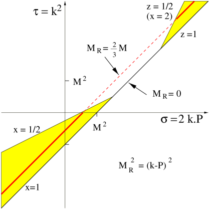
FIG. 3.: The constraint in the $\sigma-\tau$ plane coming from fixing the spectator mass $M_{R}$ (compare with Fig. 2).

The quantum numbers of the intermediate state are those determined by the action of the quark field on the state $|P,S\rangle$, hence the name diquark spectator. In the most naive picture of the quark structure of the nucleon, such that in its rest frame all quarks are in $1/2^{+}$ orbitals, the spin of the diquark system can be either 0 (scalar diquark $s$) or 1 (axial vector diquark $a$). For a pion state we have an antiquark spectator. The inclusion of antiquark and gluon distributions requires a more complex spectral decomposition of intermediate states. Here, we restrict ourselves to the simplest case. The correlation function $\Phi$ (the correlation function $\Delta$ will be treated later) is then given in the spectator model by

$$\Phi^{R}_{ij}(p,P,S)=\frac{1}{(2\pi)^{3}}\;\langle P,S|\overline{\psi}_{j}(0)|X^{(\lambda)}\rangle\;\theta(P_{R}^{+})\;\delta\left[(p-P)^{2}-M_{R}^{2}\right]\;\langle X^{(\lambda)}|\psi_{i}(0)|P,S\rangle,$$ (81)

where $P_{R}$ = $P-p$ and $X^{(\lambda)}$ represents the spectator and its possible spin states (indicated with $\lambda$). We will project onto different spins in the intermediate state and allow for different spectator masses.

We start with the correlation function $\Phi$ for a nucleon. The matrix element appearing in the RHS of (81) is given by

$$\langle X_{s}|\psi_{i}(0)|P,S\rangle={\left({i\over\hbox to0.0pt{\hbox to5.03125pt{\hfil/\hfil}\hss}p-m}\right)}_{ik}\;\Upsilon^{s}_{kl}\ U_{l}(P,S),$$ (82)

in the case of a scalar diquark, or by

$$\langle X_{a}^{(\lambda)}|\psi_{i}(0)|P,S\rangle=\epsilon_{\mu}^{*(\lambda)}{\left({i\over\hbox to0.0pt{\hbox to5.03125pt{\hfil/\hfil}\hss}p-m}\right)}_{ik}\;\Upsilon^{a\mu}_{kl}\ U_{l}(P,S),$$ (83)

for a vector diquark. The matrix elements consist of a nucleon-quark-diquark vertex $\Upsilon(N)$ yet to be specified, the Dirac spinor for the nucleon $U_{l}(P,S)$, a quark propagator for the untruncated quark line ($m$ is the constituent mass of the quark) and a polarization vector $\epsilon_{\mu}^{*(\lambda)}$ in the case of an axial vector diquark. The next step is to fix the Dirac structure of the nucleon-quark-diquark vertex $\Upsilon$. We assume the following structures:

$$\Upsilon^{s}(N)={\bf 1}\ g_{s}(p^{2}),$$ (84)

$$\Upsilon^{a\mu}(N)={g_{a}(p^{2})\over\sqrt{3}}\,\gamma_{\nu}\gamma_{5}\,\frac{\hbox to0.0pt{\hbox to7.80904pt{\hfil/\hfil}\hss}P+M}{2M}\,\left(-g^{\mu\nu}+\frac{P^{\mu}P^{\nu}}{M^{2}}\right)=\frac{g_{a}(p^{2})}{\sqrt{3}}\,\gamma_{5}\,\left(\gamma^{\mu}+\frac{P^{\mu}}{M}\right).$$ (85)

The functions $g_{\scriptscriptstyle R}(p^{2})$ (where $R$ is $s$ or $a$) are form factors that take into account the composite structure of the nucleon and the diquark spectator. In the choice of vertices, the factors and projection operators are chosen to assure that in the target rest frame, where the nucleon spinors have only upper components, the diquark spin 1 states are purely spatial and in which case the axial vector diquark vertex reduces to $\chi_{N}^{\dagger}\mbox{\boldmath$\sigma$}\cdot\mbox{\boldmath$\epsilon$}\chi_{q}$. The most general structure of the vertices can be found in [26]. With our choices, we find

$$\Phi^{R}(p,P,S)={|g_{\scriptscriptstyle R}(p^{2})|^{2}\over 2(2\pi)^{3}}\ {\delta\left(\tau-\sigma+M^{2}-M_{R}^{2}\right)\over{\left(p^{2}-m^{2}\right)}^{2}}\,(\hbox to0.0pt{\hbox to5.03125pt{\hfil/\hfil}\hss}p+m)\,\left(\hbox to0.0pt{\hbox to7.80904pt{\hfil/\hfil}\hss}P+M\right)\,(1+a_{\scriptscriptstyle R}\gamma_{5}\hbox to0.0pt{\hbox to6.70831pt{\hfil/\hfil}\hss}S)\ (\hbox to0.0pt{\hbox to5.03125pt{\hfil/\hfil}\hss}p+m),$$ (86)

where $a_{\scriptscriptstyle R}$ is a spin factor, which takes the values $a_{s}=1$ and $a_{a}=-1/3$. In obtaining this result we used as the polarization sum for the axial vector diquark in the form $\sum_{\lambda}\epsilon_{\mu}^{*(\lambda)}\epsilon_{\nu}^{(\lambda)}=-g_{\mu\nu}+P_{\mu}P_{\nu}/M^{2}$, which is consistent with the choice that the axial vector diquark spin states are purely spatial in the nucleon rest frame. We will use the same form factors for scalar and axial vector diquark:

$$g(\tau)=N\,\frac{\tau-m^{2}}{\left|\tau-\Lambda^{2}\right|^{\alpha}}.$$ (87)

The quantity $\Lambda$ is another parameter of the model which ensures that the vertex is cut off if the virtuality of the quark leg is much larger than $\Lambda^{2}$. $N$ is a normalization constant. This choice of form factor has the advantage of killing the pole of the quark propagator as suggested in [26].

In the same way, one can write down a simple spectator model for the pion. The matrix element can be written as

$$\langle X^{(\alpha)}|\psi_{i}(0)|P_{\pi}\rangle={\left({i\over\hbox to0.0pt{\hbox to5.03125pt{\hfil/\hfil}\hss}p-m}\right)}_{ik}\;\Upsilon_{kl}\ v_{l}^{(\alpha)}.$$ (88)

The spinor $v_{l}^{(\alpha)}$ describes the spin state of the antiquark spectator. The simplest vertex is given by

$$\Upsilon(\pi)=\frac{g(p^{2})}{\sqrt{2}}\,\frac{\hbox to0.0pt{\hbox to7.80904pt{\hfil/\hfil}\hss}P_{\pi}+M_{\pi}}{2M_{\pi}}\,\gamma_{5}.$$ (89)

Taking for the spectator antiquark spin sum $\sum_{\alpha}v_{l}^{(\alpha)}\bar{v}_{l}^{(\alpha)}$ = $\hbox to0.0pt{\hbox to7.80904pt{\hfil/\hfil}\hss}P_{\pi}-M_{\pi}$ one arrives at precisely the same expression as for the nucleon (Eq. (86)) with $a_{\scriptscriptstyle R}=0$.

From the correlation function $\Phi$ one easily obtains the distribution functions. Taking out the explicit $\delta$-function,

$$\Phi^{R}(p,P,S)=\tilde{\Phi}(p,P,S)\ \delta\left(\tau-\sigma+M^{2}-M_{R}^{2}\right),$$ (90)

one finds immediately from Eq. (19) the result

$$\Phi^{[\Gamma]}(x,\mbox{\boldmath$p$}_{T})=\left.\frac{{\rm Tr}(\tilde{\Phi}\Gamma)}{4(1-x)P^{+}}\right|_{\normalsize\tau=p^{2}(x,\mbox{\boldmath$p$}_{T}^{2})},$$ (91)

with

$$-p^{2}(x,\mbox{\boldmath$p$}_{T}^{2})=\frac{\mbox{\boldmath$p$}_{T}^{2}}{1-x}+\frac{x}{1-x}\,M_{R}^{2}-x\,M^{2}.$$ (92)

We now turn to the fragmentation functions. The calculation is very similar to the case of the distribution functions, involving the same type of matrix elements. Further, we assume that the hadron $h$ has no interactions with the the spectator. This allows us to use a free spinor to describe this outgoing hadron. Then we see that the correlation function $\Delta$ is the same as the one needed for the distributions, after obvious replacements in the arguments, namely

$$\Delta^{R}(k,P_{h},S_{h})={|g_{\scriptscriptstyle R}(k^{2})|^{2}\over 2(2\pi)^{3}}\ {\delta\left(\tau_{h}-\sigma_{h}+M_{h}^{2}-M_{R}^{2}\right)\over{\left(k^{2}-m^{2}\right)}^{2}}\,(\hbox to0.0pt{\hbox to5.52084pt{\hfil/\hfil}\hss}k+m)\,\left(\hbox to0.0pt{\hbox to7.80904pt{\hfil/\hfil}\hss}P_{h}+M_{h}\right)\,(1+a_{\scriptscriptstyle R}\gamma_{5}\hbox to0.0pt{\hbox to6.70831pt{\hfil/\hfil}\hss}S_{h})\,(\hbox to0.0pt{\hbox to5.52084pt{\hfil/\hfil}\hss}k+m).$$ (93)

A direct consequence is

$$\Delta^{[\Gamma]}(z,\mbox{\boldmath$k$}_{T})=\frac{1}{2z}\,\Phi^{[\Gamma^{\prime}]}\left(\frac{1}{z},\mbox{\boldmath$k$}_{T}\right)=\frac{1}{2z}\,\Phi^{[\Gamma^{\prime}]}\left(\frac{1}{z},-\,\frac{\mbox{\boldmath$k$}_{T}^{\prime}}{z}\right),$$ (94)

where $\Gamma^{\prime}$ and $\Gamma$ involve an interchange of $+$ and $-$ components. Writing $\Delta(k,P_{h},S_{h})$ = $\tilde{\Delta}(k,P_{h},S_{h})\,\delta\left((k-P_{h})^{2}-M_{R}^{2}\right)$, Eq. (55) leads to

$$\Delta^{[\Gamma]}(z,\mbox{\boldmath$k$}_{T})=\left.\frac{{\rm Tr}(\tilde{\Delta}\Gamma)}{8(1-z)P_{h}^{-}}\right|_{\normalsize\tau_{h}=k^{2}(z,\mbox{\boldmath$k$}_{T}^{2})},$$ (95)

with

$$k^{2}(z,\mbox{\boldmath$k$}_{T}^{2})=\frac{z}{1-z}\,\mbox{\boldmath$k$}_{T}^{2}+\frac{M_{R}^{2}}{1-z}+\frac{M_{h}^{2}}{z}.$$ (96)

The consequence of using free spinors to describe the outgoing hadron is that all T-odd fragmentation functions vanish and we have a one-to-one correspondence between distribution and fragmentation functions. As can be seen in Fig. 3 the actual behavior of the distribution and fragmentation functions comes from different regions in $\tau$, roughly spacelike and timelike, respectively. Therefore, the above reciprocity (Eq. (94)) is of use for the analytic expressions, less for the actual values.

IV Results and discussion

A Distribution functions of the nucleon

Using the expression in Eq. (86) we can compute the amplitudes $A_{i}$ shown in Eq. (14). Taking out some common factors by defining

$$A_{i}={N^{2}\over 2(2\pi)^{3}}\ {\delta\left(\tau-\sigma+M^{2}-M_{R}^{2}\right)\over\left|\tau-\Lambda^{2}\right|^{2\alpha}}\ \tilde{A}_{i},$$ (97)

we obtain, as expected, the T-odd amplitudes $\tilde{A}_{4}$ = $\tilde{A}_{5}$ = $\tilde{A}_{12}$ = 0, and

$$\tilde{A}_{1} = {m\over M}\,\left((M+m)^{2}-M_{R}^{2}\right)+(\tau-m^{2})\left(1+{m\over M}\right),$$ (98)

$$\tilde{A}_{2} = -\left(\tau-m^{2}\right),$$ (99)

$$\tilde{A}_{3} = (M+m)^{2}-M_{R}^{2}+(\tau-m^{2}),$$ (100)

$$\tilde{A}_{6} = -a_{\scriptscriptstyle R}\,\left[{m\over M}\,\left((M+m)^{2}-M_{R}^{2}\right)+(\tau-m^{2})\left(1+{m\over M}\right)\right],$$ (101)

$$\tilde{A}_{7} = 2\,a_{\scriptscriptstyle R}\,mM,$$ (102)

$$\tilde{A}_{8} = 2\,a_{\scriptscriptstyle R}\,M^{2},$$ (103)

$$\tilde{A}_{9} = a_{\scriptscriptstyle R}\,(\tau-m^{2}),$$ (104)

$$\tilde{A}_{10} = -a_{\scriptscriptstyle R}\,\left[(M+m)^{2}-M_{R}^{2}+(\tau-m^{2})\right],$$ (105)

$$\tilde{A}_{11} = -2\,a_{R}\,M^{2}.$$ (106)

Introducing the function $\lambda_{\scriptscriptstyle R}^{2}(x)$ such that

$$\Lambda^{2}-p^{2}=\frac{\mbox{\boldmath$p$}_{T}^{2}+\lambda_{\scriptscriptstyle R}^{2}(x)}{1-x},$$ (107)

which implies

$$\lambda_{\scriptscriptstyle R}^{2}(x)=\Lambda^{2}(1-x)+xM_{R}^{2}-x(1-x)M^{2},$$ (108)

one gets the following results for the distribution functions,

$$f_{1}(x,{\mbox{\boldmath$p$}}^{2}_{T}) = {N^{2}\,(1-x)^{2\alpha-1}\over 16\pi^{3}}\ {{\left(xM+m\right)}^{2}+{\mbox{\boldmath$p$}}_{T}^{2}\over\left({\mbox{\boldmath$p$}}_{T}^{2}+\lambda_{\scriptscriptstyle R}^{2}\right)^{2\alpha}},$$ (109)

$$g_{1L}(x,{\mbox{\boldmath$p$}}^{2}_{T}) = a_{\scriptscriptstyle R}\,{N^{2}\,(1-x)^{2\alpha-1}\over 16\pi^{3}}\ {{\left(xM+m\right)}^{2}-{\mbox{\boldmath$p$}}_{T}^{2}\over\left({\mbox{\boldmath$p$}}_{T}^{2}+\lambda_{\scriptscriptstyle R}^{2}\right)^{2\alpha}},$$ (110)

$$g_{1T}(x,{\mbox{\boldmath$p$}}^{2}_{T}) = a_{\scriptscriptstyle R}\,{N^{2}\ \,(1-x)^{2\alpha-1}\over 8\pi^{3}}\ {M(xM+m)\over\left({\mbox{\boldmath$p$}}_{T}^{2}+\lambda_{\scriptscriptstyle R}^{2}\right)^{2\alpha}},$$ (111)

$$h_{1T}(x,{\mbox{\boldmath$p$}}^{2}_{T}) = a_{\scriptscriptstyle R}\,f_{1}(x,{\mbox{\boldmath$p$}}^{2}_{T}),$$ (112)

$$h_{1L}^{\perp}(x,{\mbox{\boldmath$p$}}^{2}_{T}) = -g_{1T}(x,{\mbox{\boldmath$p$}}^{2}_{T}),$$ (114)

$$h_{1T}^{\perp}(x,{\mbox{\boldmath$p$}}^{2}_{T}) = -\,a_{\scriptscriptstyle R}\,{N^{2}\,(1-x)^{2\alpha-1}\over 8\pi^{3}}\ {M^{2}\over\left({\mbox{\boldmath$p$}}_{T}^{2}+\lambda_{\scriptscriptstyle R}^{2}\right)^{2\alpha}},$$ (116)

$$e(x,{\mbox{\boldmath$p$}}^{2}_{T}) = {N^{2}\,(1-x)^{2\alpha-2}\over 16\pi^{3}}\ {(1-x)(xM+m)(M+m)-M_{R}^{2}\left(x+{m\over M}\right)-\left(1+{m\over M}\right){\mbox{\boldmath$p$}}_{T}^{2}\over\left({\mbox{\boldmath$p$}}_{T}^{2}+\lambda_{\scriptscriptstyle R}^{2}\right)^{2\alpha}},$$ (117)

$$f^{\perp}(x,{\mbox{\boldmath$p$}}^{2}_{T}) = {N^{2}\,(1-x)^{2\alpha-2}\over 16\pi^{3}}\ {(1-x^{2})M^{2}+2mM(1-x)-M_{R}^{2}-{\mbox{\boldmath$p$}}_{T}^{2}\over\left({\mbox{\boldmath$p$}}_{T}^{2}+\lambda_{\scriptscriptstyle R}^{2}\right)^{2\alpha}},$$ (118)

$$g^{\prime}_{T}(x,{\mbox{\boldmath$p$}}^{2}_{T}) = a_{\scriptscriptstyle R}\,e(x,{\mbox{\boldmath$p$}}^{2}_{T}),$$ (119)

$$g_{L}^{\perp}(x,{\mbox{\boldmath$p$}}^{2}_{T}) = -\,a_{\scriptscriptstyle R}\,{N^{2}\,(1-x)^{2\alpha-2}\over 16\pi^{3}}\ {(1-x)^{2}M^{2}-M_{R}^{2}-{\mbox{\boldmath$p$}}_{T}^{2}\over\left({\mbox{\boldmath$p$}}_{T}^{2}+\lambda_{\scriptscriptstyle R}^{2}\right)^{2\alpha}},$$ (121)

$$g_{T}^{\perp}(x,{\mbox{\boldmath$p$}}^{2}_{T}) = a_{\scriptscriptstyle R}\,{N^{2}\,(1-x)^{2\alpha-1}\over 8\pi^{3}}\ {M^{2}\over\left({\mbox{\boldmath$p$}}_{T}^{2}+\lambda_{\scriptscriptstyle R}^{2}\right)^{2\alpha}},$$ (122)

$$h_{T}^{\perp}(x,{\mbox{\boldmath$p$}}^{2}_{T}) = a_{\scriptscriptstyle R}\,f^{\perp}(x,{\mbox{\boldmath$p$}}^{2}_{T}),$$ (123)

$$h_{L}(x,{\mbox{\boldmath$p$}}^{2}_{T}) = a_{\scriptscriptstyle R}\,{N^{2}\,(1-x)^{2\alpha-2}\over 16\pi^{3}}\ {(1-x)(xM+m)(M+m)-\left(x+{m\over M}\right)M_{R}^{2}+\left(1-2x-{m\over M}\right){\mbox{\boldmath$p$}}_{T}^{2}\over\left({\mbox{\boldmath$p$}}_{T}^{2}+\lambda_{\scriptscriptstyle R}^{2}\right)^{2\alpha}},$$ (125)

$$h_{T}(x,{\mbox{\boldmath$p$}}^{2}_{T}) = -g_{L}^{\perp}(x,{\mbox{\boldmath$p$}}^{2}_{T}).$$ (126)

Although there is a certain freedom in the choice of the parameters, one immediately sees that the occurence of singularities in the integration region (see Fig. 3) will cause problems which are avoided if there is no zero in the denominator. The requirement that $\lambda_{\scriptscriptstyle R}^{2}(x)$ is positive implies for the distribution functions ($0\leq x\leq 1$)

$$M_{R}>M-\Lambda,$$ (127)

while for the fragmentation functions (using reciprocity, we have to look at $x\geq 1$) it leads to

$$M_{R}>\Lambda-M_{h}.$$ (128)

Provided condition (127) is fulfilled, one obtains the integrated distribution functions,

$$f_{1}(x) = {N^{2}\,(1-x)^{2\alpha-1}\over 32\pi^{2}\,(\alpha-1)(2\alpha-1)}\ {2(\alpha-1)\,(xM+m)^{2}+\lambda_{\scriptscriptstyle R}^{2}(x)\over\left(\lambda_{\scriptscriptstyle R}^{2}(x)\right)^{2\alpha-1}},$$ (129)

$$g_{1}(x) = {N^{2}a_{\scriptscriptstyle R}\,(1-x)^{2\alpha-1}\over 32\pi^{2}\,(\alpha-1)(2\alpha-1)}\ {2(\alpha-1)\,(xM+m)^{2}-\lambda_{\scriptscriptstyle R}^{2}(x)\over\left(\lambda_{\scriptscriptstyle R}^{2}(x)\right)^{2\alpha-1}},$$ (130)

$$h_{1}(x) = {N^{2}a_{\scriptscriptstyle R}\,(1-x)^{2\alpha-1}\over 16\pi^{2}(2\alpha-1)}\ {(xM+m)^{2}\over\left(\lambda_{\scriptscriptstyle R}^{2}(x)\right)^{2\alpha-1}},$$ (131)

$$e(x) = {N^{2}\,(1-x)^{2\alpha-2}\over 32\pi^{2}(\alpha-1)(2\alpha-1)}\ {2(\alpha-1)\left(x+{m\over M}\right)\left[(1-x)(M+m)M-M_{R}^{2}\right]-\left(1+{m\over M}\right)\lambda_{\scriptscriptstyle R}^{2}(x)\over\left(\lambda_{\scriptscriptstyle R}^{2}(x)\right)^{2\alpha-1}},$$ (132)

$$g_{T}(x) = {N^{2}a_{\scriptscriptstyle R}\,(1-x)^{2\alpha-2}\over 32\pi^{2}(\alpha-1)(2\alpha-1)}\ {2(\alpha-1)\left(x+{m\over M}\right)\left[(1-x)(M+m)M-M_{R}^{2}\right]-\left(x+{m\over M}\right)\lambda_{\scriptscriptstyle R}^{2}(x)\over\left(\lambda_{\scriptscriptstyle R}^{2}(x)\right)^{2\alpha-1}},$$ (133)

$$h_{L}(x) = {N^{2}a_{\scriptscriptstyle R}\,(1-x)^{2\alpha-2}\over 32\pi^{2}(\alpha-1)(2\alpha-1)}\ {2(\alpha-1)\left(x+{m\over M}\right)\left[(1-x)\left(M+m\right)M-M_{R}^{2}\right]+\left(1-2x-{m\over M}\right)\lambda_{\scriptscriptstyle R}^{2}(x)\over\left(\lambda_{\scriptscriptstyle R}^{2}(x)\right)^{2\alpha-1}}.$$ (134)

Examples of the $\mbox{\boldmath$p$}_{T}^{2}/2M^{2}$-weighted distributions are

$$g_{1T}^{(1)}(x)=-h_{1L}^{\perp(1)}(x)={N^{2}a_{\scriptscriptstyle R}\,(1-x)^{2\alpha-1}\over 32\pi^{2}\,(\alpha-1)(2\alpha-1)}\ {x+{m\over M}\over\left(\lambda_{\scriptscriptstyle R}^{2}(x)\right)^{2\alpha-2}}.$$ (135)

We note that these latter functions do not vanish at $x=0$, implying non-vanishing sum rules for $g_{2}$ and $h_{2}$, in accordance with Eqs. (53) and (54), except if the quarks are massless.

The functions $g_{2}$ and $h_{2}$ are given by

$$g_{2}(x)={h_{2}(x)\over 2}={N^{2}a_{\scriptscriptstyle R}\ (1-x)^{2\alpha-2}\over 32\pi^{2}\,(\alpha-1)(2\alpha-1)}\ {2(\alpha-1)\left(x+{m\over M}\right)\left[M^{2}(1-x)^{2}-M_{R}^{2}\right]+\left(1-2x-{m\over M}\right)\lambda_{\scriptscriptstyle R}^{2}(x)\over\left(\lambda_{\scriptscriptstyle R}^{2}(x)\right)^{2\alpha-1}}.$$ (136)

We can directly check that Eqs. (50) and (51) are satisfied.

Up to now, we have not specified flavor in the distributions. For the nucleon we only distinguished two types of distributions, $f_{1}^{s}$ and $f_{1}^{a}$, etc. Since spin 0 diquarks are in a flavor singlet state and spin 1 diquarks are in a flavor triplet state, in order to combine to a symmetric spin-flavor wave function as demanded by the Pauli principle, the proton wave function has the well-known $SU(4)$ structure,

$$|p\uparrow\rangle={1\over\sqrt{2}}\ |u\uparrow S_{0}^{0}\rangle+{1\over\sqrt{18}}|u\uparrow A_{0}^{0}\rangle-{1\over 3}\ |u\downarrow A_{0}^{1}\rangle-{1\over 3}\ |d\uparrow A_{1}^{0}\rangle+\sqrt{{2\over 9}}\ |d\downarrow A_{1}^{1}\rangle,$$ (137)

where $S$ ($A$) represents a scalar (axial vector) diquark and the upper (lower) indices represent the projections of the spin (isospin) along a definite direction. Since the coupling of the spin has already been included in the vertices, we need the flavor coupling

$$|p\rangle={1\over\sqrt{2}}\ |u\ S_{0}\rangle+{1\over\sqrt{6}}|u\ A_{0}\rangle-{1\over\sqrt{3}}\ |d\ A_{1}\rangle,$$ (138)

to find that for the nucleon the flavor distributions are

$$f_{1}^{u}=\frac{3}{2}\,f_{1}^{s}+\frac{1}{2}\,f_{1}^{a},$$ (139)

$$f_{1}^{d}=f_{1}^{a},$$ (140)

and similarly for the other functions. The proportionality of the numbers is obtained from Eq. (138), while the overall factor is chosen to reproduce the sum rules for the number of up and down quarks if $f_{1}^{s}$ and $f_{1}^{a}$ are normalized to unity upon integration over $\mbox{\boldmath$p$}_{T}$ and $x$. This will fix the normalization $N$ in the form factor in Eq. (87). Notice that the factors $a_{s}=1$ and $a_{a}=-1/3$ in the distribution functions will produce different $u$ and $d$ weighting for unpolarized and polarized distributions. Further differences between $u$ and $d$ distributions can also be induced by different choices of $M_{R}$, $\Lambda$ or $\alpha$. We take for the nucleon $\alpha=2$ to reproduce the right large $x$ behavior of $f_{1}^{u}$, i.e. $(1-x)^{3}$, as predicted by the Drell-Yan-West relation and reasonably well confirmed by data. We refrain from tuning the large $x$ behavior of $f_{1}^{d}$ to match the $(1-x)^{4}$ form indicated by data. Since $f_{1}^{d}$ is only affected by vector diquarks, this could be easily obtained by choosing a different form factor for the latter. We feel that this kind of fine-tuning would take things too far with the simple model we use. Similarly, we will only consider one common value for $\Lambda$. We will, however, consider different masses for scalar and vector diquark spectators. The color magnetic hyperfine interaction, held responsible for the nucleon-delta mass difference of 300 MeV, will also produce a mass difference between singlet and triplet diquark states. Neglecting dynamical effects, group-theoretical factors lead to a difference $M_{a}-M_{s}$ = 200 MeV [27].

Another important constraint comes from the axial charge of the nucleon, given by

$$g_{\scriptscriptstyle A}=\int_{0}^{1}dx\left[g_{1}^{u}(x)-g_{1}^{d}(x)\right]=\int_{0}^{1}dx\left[{3\over 2}\ g_{1}^{s}(x)-{1\over 2}\ g_{1}^{a}(x)\right].$$ (141)

The sensitivity to the parameters $M_{R}$ and $\Lambda$ is best illustrated by considering some characteristic values. We take a quark mass of 0.36 GeV (about one third of the average nucleon-delta mass), two different values for $M_{R}$ (0.6 and 0.8 GeV) and three values for $\Lambda$ (0.4, 0.5 and 0.6 GeV). The distributions turn out to be insensitive to the value chosen for the quark mass. In Table I the values of some moments are given.

TABLE I.: The second moment of $f_{1}$, $\langle x\rangle$ = $\int dx\,xf_{1}(x)$ and the first moments $g_{1}$ = $\int dx\,g_{1}(x)$ and $h_{1}$ = $\int dx\,h_{1}(x)$ are given for two diquark masses and for three values of $\Lambda$.

	$M_{R}=0.6$ GeV			$M_{R}=0.8$ GeV
$\Lambda$ (GeV)	$\langle x\rangle^{R}$	$g_{1}^{R}$	$h_{1}^{R}$	$\langle x\rangle^{R}$	$g_{1}^{R}$	$h_{1}^{R}$
0.4	0.366	0.923$\,a_{R}$	0.962$\,a_{R}$	0.230	0.650$\,a_{R}$	0.825$\,a_{R}$
0.5	0.375	0.794$\,a_{R}$	0.897$\,a_{R}$	0.256	0.527$\,a_{R}$	0.764$\,a_{R}$
0.6	0.384	0.671$\,a_{R}$	0.835$\,a_{R}$	0.277	0.416$\,a_{R}$	0.708$\,a_{R}$

TABLE II.: The second moment of $f_{1}$, $\langle x\rangle$ = $\int dx\,xf_{1}(x)$ and the first moments $g_{1}$ = $\int dx\,g_{1}(x)$ and $h_{1}$ = $\int dx\,h_{1}(x)$ are given for $u$ and $d$ quarks in a proton for three values of $\Lambda$.

	$u$-quark			$d$-quark
$\Lambda$ (GeV)	$\langle x\rangle^{u}$	$g_{1}^{u}$	$h_{1}^{u}$	$\langle x\rangle^{d}$	$g_{1}^{d}$	$h_{1}^{d}$
0.4	$0.664$	$1.277$	$1.305$	$0.230$	$-0.217$	$-0.275$
0.5	$0.690$	$1.103$	$1.218$	$0.256$	$-0.176$	$-0.255$
0.6	$0.715$	$0.937$	$1.135$	$0.277$	$-0.139$	$-0.236$

Fig. 4 shows the twist two distributions for different values of the mass of the spectator and of the parameter $\Lambda$. Clearly, $M_{R}$ dictates the position of the maximum, while $\Lambda$ governs the width of the distribution. We can see that an increase of $M_{R}$ induces a shift on the peak of the valence distribution $f_{1}(x)$ towards lower values of $x$ and a decrease in its second moment. In order to model sea quark distributions, one could introduce heavier spectators with four quarks or three quarks and one antiquark, and in this way satisfy the momentum sum rule at the model-scale. In the absence of transverse momentum for the quarks he have $f_{1}(x)=g_{1}(x)/a_{R}=h_{1}(x)/a_{R}$.

FIG. 4.: Twist two distributions for the nucleon. The plots on the top represent $f_{1}(x)$, the ones on the middle show $g_{1}(x)/a_{R}$ and at the bottom we have $h_{1}(x)/a_{R}$. The plots on the left correspond to $\Lambda=0.4$ GeV and the ones on the right to $\Lambda=0.6$ GeV. The full line corresponds to $M_{R}=0.6$ GeV and the dashed line to $M_{R}=0.8$ GeV.

In Table II we have given the values of some moments for $u$ and $d$ quarks in the proton using $M_{s}=0.6$ GeV and $M_{a}=0.8$ GeV.We now use the axial charge of the nucleon, $g_{A}=g_{1}^{u}-g_{1}^{d}$, to find the most suitable values for $\Lambda$. The value $\Lambda=0.5$ GeV gives $g_{\scriptscriptstyle A}=1.28$, close to the experimental value.

FIG. 5.: Twist two distributions for the nucleon. The plot at the top shows $xf_{1}^{s}(x)$ (full line) and $xf_{1}^{a}(x)$ (dashed line) for $M_{s}=0.6$ GeV, $M_{a}=0.8$ GeV and $\Lambda=0.5$ GeV. The plot on the middle shows $xf_{1}^{u}(x)$ (full line) and $xf_{1}^{d}(x)$ (dashed line) for the same values of the parameters. The third plot shows the low scale ($\mu^{2}=0.23$ GeV²) valence distributions of Glück, Reya and Vogt [28].

Fig. 5 shows the distribution $f_{1}(x)$ multiplied by $x$. We find a satisfactory qualitative agreement with the valence distributions of Glück, Reya and Vogt (GRV) calculated at the low scale $\mu^{2}_{LO}=0.23$ GeV² [28]. For $u$ and $d$ quarks, the first moment of $f_{1}(x)$ is clearly larger in our model, which would imply that our results describe the nucleon at an even lower scale than GRV. Fig. 6 shows the distributions $g_{1}^{u}(x)$ and $g_{1}^{d}(x)$ multiplied by $x$ for the values $M_{s}=0.6$ GeV, $M_{a}=0.8$ GeV and $\Lambda=0.5$ GeV. Again, we find a qualitative agreement with the polarized valence distributions of Glück et al. [29]. Using the same parameters, we can obtain higher twist distributions. Fig. 7 shows the twist three distributions $e^{u}(x)$ and $e^{d}(x)$, Fig. 8 shows the distributions $g_{1T}^{(1)u}(x)$ and $g_{1T}^{(1)d}(x)$, while in Fig. 9 we have the distributions $g_{2}^{u}(x)$ and $g_{2}^{d}(x)$. We find a small violation of the Burkhardt-Cottingham sum rule, in agreement with Eq. (53), due to the non-zero value of $g_{1T}^{(1)}(0)$.

FIG. 6.: Polarized proton distributions $g_{1}^{u}(x)$ and $g_{1}^{d}(x)$. The first plot shows our estimates for $xg_{1}^{u}(x)$ (full line) and $xg_{1}^{d}(x)$ (dashed line) for $\Lambda=0.5$ GeV, $M_{s}=0.6$ GeV and $M_{a}=0.8$ GeV. The second plot shows the low scale $\mu_{LO}^{2}=0.23$ GeV² parametrization of Glück, et al. [29] for the same functions

.

FIG. 7.: Distributions $e^{u}(x)$ (solid line) and $e^{d}(x)$ (dotted line) for $M_{s}=0.6$ GeV, $M_{a}=0.8$ GeV and $\Lambda=0.5$ GeV.

FIG. 8.: Distributions $g_{1T}^{(1)u}(x)$ (solid line) and $g_{1T}^{(1)d}(x)$ (dashed line) for $M_{s}=0.6$ GeV, $M_{a}=0.8$ GeV and $\Lambda=0.5$ GeV.

FIG. 9.: Distributions $g_{2}^{u}(x)$ (solid line) and $g_{2}^{d}(x)$ (dashed line) for $M_{s}=0.6$ GeV, $M_{a}=0.8$ GeV and $\Lambda=0.5$ GeV.

At this point it is important to realize that in this model there are no antiquarks. This means that the distribution functions are zero for $x<0$, due to the symmetry properties of the matrix elements involved in the calculation. Therefore, $C$-even and $C$-odd sum rules are equal.

B Distribution functions for the pion

The expressions for the distribution functions for the pion are the same as those for the nucleon with $a_{R}=0$ and making the replacement $M_{R}\rightarrow m$. Only spin independent functions will remain. For $\alpha=1$ we have $f_{1}(x)=2(1-x)$, showing the power law behavior expected from simple counting rules. The apparent singularity caused by the factor $(\alpha-1)$ that enters in the denominator can be avoided including this factor in the normalization $N$. In this case we find the symmetry $x\leftrightarrow(1-x)$ for $xf_{1}(x)$. For values of $\alpha$ different from 1 the functions depend on the parameter $\Lambda$, which is constrained by Eq. (127). For $\Lambda=0.4$ GeV, the distribution $f_{1}(x)$ is shown in Fig. 10 for two values of $\alpha$ and compared with the parametrization of the leading order valence distributions of Glück, Reya and Vogt at the low scale $\mu^{2}_{LO}=0.25$ GeV² [30].

In this case the vertex gives immediately identical antiquark distribution or, equivalently, a contribution for negatives values of $x$.

FIG. 10.: Momentum distribution $xf_{1}(x)$ for the pion for $\alpha=1.0$ (solid line) and $\alpha=1.2$, $\Lambda=0.4$ GeV (dashed line). The dotted line represents the GRV low scale parametrization [30].

C Fragmentation functions for the nucleon

The assumed form of the quark-diquark-nucleon vertex also allows the calculation of the fragmentation functions for the nucleons. We can use the reciprocity relation mentioned at the end of section III to obtain the analytic expressions for $D_{1}(z,-z{\mbox{\boldmath$k$}}_{T})$, etc., and, after integration over ${\mbox{\boldmath$k$}}^{\prime}_{T}=-z{\mbox{\boldmath$k$}}_{T}$, the expressions for $D_{1}(z)$ etc. In this case we introduce the function $\lambda_{\scriptscriptstyle R}$ through the relation

$$k^{2}-\Lambda^{2}={{\mbox{\boldmath$k$}}_{T}^{2}+\lambda_{\scriptscriptstyle R}^{2}(1/z)\over 1-z}.$$ (142)

For example, the unpolarized fragmentation function reads

$$D_{1}(z,z^{2}{\mbox{\boldmath$k$}}_{T}^{2})={N_{F}^{2}(1-z)^{2\alpha-1}\over 16\pi^{3}z^{2\alpha}}\ {\left({M\over z}+m\right)^{2}+{\mbox{\boldmath$k$}}_{T}^{2}\over\left({\mbox{\boldmath$k$}}_{T}^{2}+\lambda_{\scriptscriptstyle R}^{2}\left({1\over z}\right)\right)^{2\alpha}},$$ (143)

and, after integration over the transverse momentum,

$$zD_{1}(z)={N_{F}^{2}\,z^{2\alpha-1}\,(1-z)^{2\alpha-1}\over 32\pi^{2}\,(\alpha-1)(2\alpha-1)}\ {2(\alpha-1)\,(M+mz)^{2}+z^{2}\,\lambda_{\scriptscriptstyle R}^{2}\left({1\over z}\right)\over\left(z^{2}\lambda_{\scriptscriptstyle R}^{2}\left({1\over z}\right)\right)^{2\alpha-1}}.$$ (144)

The factor $N_{F}$ is a normalization constant. Distinguishing $D_{1}^{s}(D_{1}^{a})$ as the fragmentation functions for a quark into a nucleon and an anti-S diquark (anti-$A$ diquark), one finds

$$D_{1}^{u\rightarrow p} = {3\over 2}\ D_{1}^{s}+{1\over 2}D_{1}^{a},$$ (145)

$$D_{1}^{u\rightarrow n} = D_{1}^{d\rightarrow p}=D_{1}^{a},$$ (146)

and similarly for $G_{1}$ and $H_{1}$. In this case there is no sum rule to fix the normalizations of $D_{1}^{s}$ and $D_{1}^{a}$. In the $SU(4)$ symmetric limit $(D_{1}^{s}=D_{1}^{a})$, one finds the expected ratio $D_{1}^{u\rightarrow p}/D_{1}^{d\rightarrow p}=2$. We will introduce the scale invariant quantities

$$\epsilon^{\scriptscriptstyle R}=\int_{0}^{1}dz\,z\,D_{1}^{R}(z),$$ (147)

and express our results with the help of these quantities. In Table III the values of some moments are given for a quark mass of 0.36 GeV, two different values of $M_{R}$ (0.6 and 0.8 GeV) and three values of $\Lambda$ (0.4, 0.5 and 0.6 GeV.) By normalizing $\epsilon^{s}=\epsilon^{a}=1$, we obtain the results for $u$ and $d$ quarks given in Table IV.

TABLE III.: The first two moments of the unpolarized fragmentation function $D_{1}^{R}$ ($N^{R}=\int D_{1}^{R}(z)\,dz$ and $\epsilon^{R}$) and the ratios $G_{1}^{R}/N^{R}=\int G_{1}^{R}(z)\,dz/N^{R}$ and $H_{1}^{R}/N^{R}=\int H_{1}^{R}(z)\,dz/N^{R}$ for different values of $\Lambda$ and $M_{R}$.

	$M_{R}=0.6$ GeV				$M_{R}=0.8$ GeV
$\Lambda$ (GeV)	$N^{R}$	$\epsilon^{R}$	$G_{1}^{R}/N^{R}$	$H_{1}^{R}/N^{R}$	$N_{R}$	$\epsilon^{R}$	$G_{1}^{R}/N^{R}$	$H_{1}^{R}/N^{R}$
0.4	$1.908\;\epsilon^{\scriptscriptstyle R}$	$2.732\times 10^{-5}$	$0.628\;a_{\scriptscriptstyle R}$	$0.814\;a_{\scriptscriptstyle R}$	$2.112\;\epsilon^{\scriptscriptstyle R}$	$3.785\times 10^{-4}$	$0.538\;a_{\scriptscriptstyle R}$	$0.769\;a_{\scriptscriptstyle R}$
0.5	$1.901\;\epsilon^{\scriptscriptstyle R}$	$4.808\times 10^{-4}$	$0.639\;a_{\scriptscriptstyle R}$	$0.820\;a_{\scriptscriptstyle R}$	$2.107\;\epsilon^{\scriptscriptstyle R}$	$1.345\times 10^{-3}$	$0.548\;a_{\scriptscriptstyle R}$	$0.774\;a_{\scriptscriptstyle R}$
0.6	$1.891\>\epsilon^{\scriptscriptstyle R}$	$2.429\times 10^{-3}$	$0.654\;a_{\scriptscriptstyle R}$	$0.827\;a_{\scriptscriptstyle R}$	$2.099\;\epsilon^{\scriptscriptstyle R}$	$3.732\times 10^{-3}$	$0.561\;a_{\scriptscriptstyle R}$	$0.781\;a_{\scriptscriptstyle R}$

TABLE IV.: The first two moments of the $u$ and $d$ quark combinations of Eqs. (145) and (146) and the ratios $G_{1}^{q}/N^{q}=\int G_{1}^{q}(z)\,dz/N^{q}$ and $H_{1}^{q}/N^{q}=\int H_{1}^{q}(z)\,dz/N^{q}$ for fragmentation into protons.

	$u$-quark				$d$-quark
$\Lambda$ (GeV)	$N^{u}$	$\epsilon^{u}$	$G_{1}^{u}/N^{u}$	$H_{1}^{u}/N^{u}$	$N^{d}$	$\epsilon^{d}$	$G_{1}^{d}/N^{d}$	$H_{1}^{d}/N^{d}$
0.4	$3.917$	$2$	$0.410$	$0.525$	$2.112$	$1$	$-0.179$	$-0.256$
0.5	$3.904$	$2$	$0.418$	$0.529$	$2.107$	$1$	$-0.183$	$-0.258$
0.6	$3.886$	$2$	$0.427$	$0.533$	$2.099$	$1$	$-0.187$	$-0.260$

In Fig. 11 we show our results for the unpolarized fragmentation function $D_{1}$ and the ratios of polarized to unpolarized functions $G_{1}(z)/D_{1}(z)$ and $H_{1}(z)/D_{1}(z)$. Since the dependence on the parameter $\Lambda$ turns out to be weak, we display results for the choice $\Lambda=0.5$ GeV only. On the left hand side of the figure the two spectator masses ($M_{R}=0.6$ GeV and $M_{R}=0.8$ GeV) are compared. On the right hand side we show the results for the $u$ and the $d$ quark fragmentation functions as defined by Eqs. (145) and (146). To allow a comparison with data [31] we fixed the normalization such that the second moment $\epsilon^{q\to p}=\int dz\,z\,D_{1}^{q}(z)$ takes the value

$$\int dz\,z\,\left(D_{1}^{u\to p}(z)-D_{1}^{u\to\bar{p}}(z)\right)\approx 0.019,$$ (148)

which is our (rough) estimate for the second moment obtained from the EMC data. We compare our result for $D_{1}^{u}(z)$ to the difference

$$D_{1}^{u\to p}(z)-D_{1}^{u\to\bar{p}}(z)=D_{1}^{u\to p}(z)-D_{1}^{\bar{u}\to p}(z),$$ (149)

since it is the appropriate combination for comparison with a model involving only valence quarks, although in our model $D_{1}^{u\to\bar{p}}$ is zero by construction (as are all so-called unfavored fragmentation functions). Furthermore, since in the EMC analysis the assumption $D_{1}^{u\to p}(z)=D_{1}^{d\to p}(z)$ was made, we compare our result for $D_{1}^{d}(z)$ to just the same combination of Eq. (149). The ratios of polarized to unpolarized fragmentation functions, $G_{1}(z)/D_{1}(z)$ and $H_{1}(z)/D_{1}(z)$, are given for the $q=u,d$ as well; normalization factors drop from the ratios.

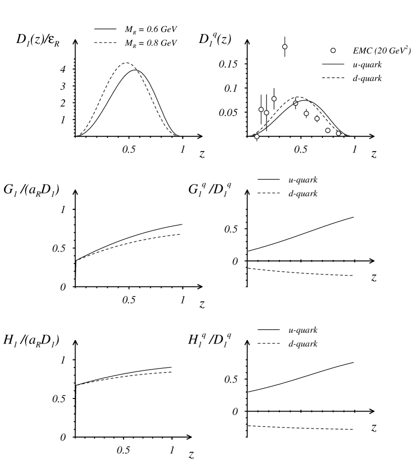
FIG. 11.: Twist two fragmentation functions. The plots on the left show $D_{1}^{R}(z)/\epsilon^{R}$ (with $\epsilon^{R}$ defined according to Eq. (147)) and the ratios $G_{1}(z)/(a_{R}D_{1}^{R}(z))$ and $H_{1}(z)/(a_{R}D_{1}^{R}(z))$ for $M_{R}=0.6$ GeV and $M_{R}=0.8$ GeV ($\Lambda=0.5$ GeV). The plots on the right show the $u$ and $d$ quark results obtained with $\epsilon^{s}=\epsilon^{a}=1$. For comparison with data our results for $D_{1}^{q}(z)$ are rescaled (see text). Data for the difference $(D_{1}^{u\to p}(z)-D_{1}^{u\to\bar{p}}(z))$ are taken from [31].

D Fragmentation functions for the pion

Our results for the fragmentation function of a quark to a pion are shown in Fig. 12. We display $zD_{1}^{u\to\pi^{+}}(z)$ which is rescaled such that the second moment $\epsilon^{q\to\pi}=\int dz\,z\,D_{1}^{u\to\pi^{+}}(z)$ equals the value of the valence combination

$$\int dz\,z\,\left(D_{1}^{u\to{\pi^{+}}}(z)-D_{1}^{u\to{\pi^{-}}}(z)\right)\approx 0.088,$$ (150)

our estimate for the second moment obtained from the corresponding EMC data [31] (more recent parametrizations available for the combination ($D_{1}^{u\to{\pi^{+}}}+D_{1}^{u\to{\pi^{-}}}$) [32] agree with the EMC data).

Note that in our calculation all favored fragmentation functions are identical

$$D_{1}^{u\to{\pi^{+}}}(z)=D_{1}^{\bar{d}\to{\pi^{+}}}(z)=D_{1}^{d\to{\pi^{-}}}(z)=D_{1}^{\bar{u}\to{\pi^{-}}}(z),$$ (151)

while all unfavored fragmentation functions have not been considered in our approach:

$$D_{1}^{d\to{\pi^{+}}}(z)=D_{1}^{\bar{u}\to{\pi^{+}}}(z)=D_{1}^{\bar{d}\to{\pi^{-}}}(z)=D_{1}^{u\to{\pi^{-}}}(z)=0.$$ (152)

The latter property has to be contrasted with the experimental observation that unfavored fragmentation functions can be as large as the favored ones for small $z$, are suppressed by a factor of about 2 for $0.4\leq z\leq 0.6$ and even stronger suppressed for large $z$ [31]. This observation holds true for both nucleons and pions.

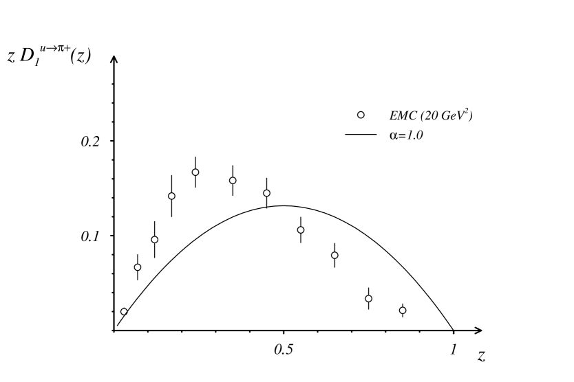
FIG. 12.: The pion fragmentation function $z\,D_{1}^{u\to{\pi^{+}}}(z)$ (rescaled, see text) for $\alpha=1.0$ is compared to the EMC data from Ref. [31]. Data are shown for the difference ($z\,D_{1}^{u\to{\pi^{+}}}-z\,D_{1}^{u\to{\pi^{-}}}$).

E Summary

In this paper we combined the representation of distribution and fragmentation functions in terms of non-local operator expectation values with a simple spectator model. This amounts to saturating the antiquark-hadron intermediate state with one single state of definite mass. With an effective vertex that connects to this state, containing a form factor, we can calculate all the independent amplitudes that are allowed for the non-local operator expectation values after imposing constraints of Lorentz invariance and invariance under parity and time-reversal operations. Exploiting the explicit expressions of distribution and fragmentation functions in terms of those amplitudes, several relations between $p_{T}$-integrated distribution (or fragmentation) functions arise.

For nucleons and pions we have obtained expressions for the distribution and fragmentation functions within our approach. Flavor charges and axial vector charge served to fix the free parameters of the model in the case of the distribution functions. For the fragmentation functions we utilized the same set of parameters except for the overall normalization which in this case is not constrained by a number sum-rule. Considering all Dirac projections in leading and subleading order (in an expansion in 1/Q) we were able to give estimates for the polarized and unpolarized cases, including subleading (higher twist) functions. The latter lack a simple probabilistic interpretation, but are well defined as projections of non-local operators.

By comparing our expressions to available parametrizations at ‘low (hadronic) scales’ and to some experimental data we find that we can obtain reasonable qualitative agreement for the unpolarized distribution function $f_{1}(x)$, the longitudinal spin-distribution $g_{1}(x)$ and with the unpolarized fragmentation function $D_{1}(z)$ for both nucleons and pions. These findings give confidence that the estimates obtained for the ‘terra incognita’ functions (transverse spin distributions, longitudinal and transverse spin fragmentations and subleading functions) provide a reasonable estimate of the order of magnitude of the functions and their (large) $x$ behavior despite the simplicity of the model. The comparison to the available parametrizations and experimental data gives an indication of the level of accuracy our estimates can reach, keeping in mind that we have excluded the sea-quark and gluon sectors, and evolution.

- [1] D.E. Soper, Phys. Rev. D 15, 1141 (1977); Phys. Rev. Lett. 43, 1847 (1979).
- [2] J.C. Collins and D.E. Soper, Nucl. Phys. B194, 445 (1982).
- [3] R.L. Jaffe, Nucl. Phys. B229, 205 (1983).
- [4] X. Song and J.S. McCarthy, Phys. Rev. D 49, 3169 (1994).
- [5] R.L. Jaffe, Phys. Rev. D 11, 1953 (1975).
- [6] C.J. Benesh and G.A. Miller, Phys. Lett. B 215, 381 (1988).
- [7] A.W. Schreiber, A.I. Signal and A.W. Thomas, Phys. Rev. D 44, 2653 (1991).
- [8] M. Ropele, M. Traini and V. Vento, Nucl. Phys. A584, 227 (1995).
- [9] R.G. Roberts and G.G. Ross, Phys. Lett. B 373, 235 (1996).
- [10] V. Barone, T. Calarco and A. Drago, Phys. Lett. B 390, 287 (1997).
- [11] H. Weigel, L. Gamberg and H. Reinhardt, hep-ph/9604295.
- [12] H. Weigel, L. Gamberg and H. Reinhardt, hep-ph/9609226.
- [13] D.I. Diakonov, et al., hep-ph/9703420.
- [14] C.J. Benesh and G.A. Miller, Phys. Rev. D 36, 1344 (1987).
- [15] H. Meyer and P.J. Mulders, Nucl. Phys. A528, 589 (1991).
- [16] J. Rodrigues, A. Henneman and P.J. Mulders, in Proceedings of the First ELFE Summer School on Confinement Physics, Cambridge, UK, 1995, eds. S.D. Bass and P.A.M. Guichon (Editions Frontières, 1996).
- [17] M. Nzar and P. Hoodbhoy, Phys. Rev. D 51, 32 (1995).
- [18] Y. Koike and N. Nishiyama, Phys. Rev. D 55, 3068 (1997), and references therein.
- [19] J.P. Ralston and D.E. Soper, Nucl. Phys. B152, 109 (1979).
- [20] R.D. Tangerman and P.J. Mulders, Phys. Rev. D 51, 3357 (1995).
- [21] P.J. Mulders and R.D. Tangerman, Nucl. Phys. B461, 197 (1996).
- [22] H. Burkhardt and W.N. Cottingham, Ann. Phys. (N.Y.) 56, 453 (1970).
- [23] M. Burkardt, in Proceedings of 10th International Symposium on High Energy Spin Physics, Nagoya, Japan, 1992, ed. Hasegawa et al. (Universal Academy Press, Tokyo, 1993).
- [24] M. Burkardt; Phys. Rev. D 52, 3841 (1995).
- [25] D. Boer, R. Jakob and P.J. Mulders; hep-ph/9702281.
- [26] W. Melnitchouk, A.W. Schreiber and A.W. Thomas, Phys. Rev. D 49, 1183 (1994).
- [27] F.E. Close and A.W. Thomas; Phys. Lett. B 212, 227 (1988).
- [28] M. Glück, E. Reya and A. Vogt; Z. Phys. C 67, 433 (1995).
- [29] M. Glück, et al.; Phys. Rev. D 53, 4775 (1996).
- [30] M. Glück, E. Reya and A. Vogt; Z. Phys. C 53, 651 (1992).
- [31] M. Arneodo, et al., European Muon Collaboration; Nucl. Phys. B321, 541 (1989).
- [32] J. Binnewies, B.A. Kniehl and G. Kramer, Z. Phys. C 65, 471 (1995).