Abstract

We discuss the new model expression $\bar{\alpha}_{\rm an}(Q^{2})$ recently obtained for the QCD running coupling with a regular ghost-free behavior in the “low $Q^{2}$” region. Being deduced from the standard “asymptotic-freedom” expression by imposing the $Q^{2}$-analyticity – without any adjustable parameters – it obeys nice features: (i) The universal limiting value $\bar{\alpha}_{\rm an}(0)=4\pi/\beta_{0}\simeq 1.4$ expressed only via group symmetry factors and independent of experimental estimates on the running coupling $\bar{\alpha}_{s}(Q^{2})$ (of QCD scale parameter $\Lambda$). This value turns out to be stable with respect to higher order corrections; (ii) Stability of IR behavior with respect to higher-loop effects; (iii) Coherence between the experimental $\bar{\alpha}_{\rm an}(M_{\tau}^{2})$ value and integral information on IR $\bar{\alpha}_{s}(Q^{2})$ behavior as extracted from jet physics data.

The ghost-pole problem in the behavior of a running coupling, being an obvious property of the geometrical progression, spoils a physical discussion of the RG-summed perturbative QCD results in the infrared (IR) region. To avoid it, one uses some artificial constructions like the “freezing of the coupling” hypothesis.

Here, we are going to revive an old idea of combining the RG summation with analyticity in the $Q^{2}$ variable. It was successfully used in the late 50’s for examining the QED ghost-pole issue [1, 2]. Quite recently, it has been proposed for applying to the QCD case [3].

The QED effective coupling $\bar{\alpha}(Q^{2})$ being proportional to the transverse dressed-photon propagator amplitude according to general principles of local QFT satisfies the Käll$\acute{{\rm e}}$n–Lehmann spectral representation and, therefore, is an analytic function in the cut complex $Q^{2}$ plane.

The “analytization procedure” elaborated in papers [1, 2] consists of three steps:

(I) To find an explicit expression for $\bar{\alpha}_{RG}(Q^{2})$ in the Euclidean region $Q^{2}>0$ by standard RG improvement of a perturbative input.

(II) To perform the straightforward analytical continuation of this expression into the Minkowskian region ${\rm Re}\,Q^{2}<0$, ${\rm Im}\,Q^{2}=-\epsilon$. To calculate its imaginary part and to define the spectral density by $\rho_{RG}(\sigma,\alpha)={\rm Im}\bar{\alpha}_{RG}(-\sigma-i\epsilon,\alpha)$.

(III) Using the spectral representation [see Eq. (2) below] with $\rho_{RG}$ in the integrand to define an “analytically-improved” running coupling $\bar{\alpha}_{{\rm an}}(Q^{2})$ in the Euclidean region.

Being applied to $\bar{\alpha}(Q^{2})$ in the one-loop ultra-violet (UV) QED case, this procedure produced [2] an explicit expression with the following properties:

(a) it has no ghost pole,

(b) as a function of $\alpha$ at the point $\alpha=0$ it possesses an essential singularity

$\sim~{}\exp(-3\pi/\alpha)$,

(c) in the vicinity of this singularity for real and positive $\alpha$ it admits a power expansion that coincides with the perturbation one (used as an input),

(d) it has the finite UV limit $\bar{\alpha}(\infty,\alpha)=3\pi$ that does not depend on the experimental value $\alpha\simeq 1/137$.

The same procedure being applied to the two-loop QED case yielded [2] a more complicated expression with the same essential features.

In the QCD case, to apply this technique to the strong running coupling, one has to make two reservations.

First, as far as here $\bar{\alpha}_{s}(Q^{2})$ is defined via a product of propagators and a vertex function, there is a question about validity of the spectral representation. Happily, this point has been discussed in paper [4]. As a result, one can use the Käll$\acute{{\rm e}}$n-Lehmann analyticity here, as well.

Second, in QCD, the running of coupling is, generally, connected with the running of gauge. For simplicity, we assume that the $\overline{{\rm MS}}$ scheme is used (or the MOM scheme in the transverse gauge) when $\bar{\alpha}_{s}$ is not influenced by the running of gauge.

To construct an analytic effective coupling in the QCD case, we start with the leading-logs expression

$$\bar{a}^{(1)}(Q^{2})=\frac{a}{1+a\beta_{0}\ln(Q^{2}/\mu^{2})}=\frac{1}{\beta_{0}\ln(Q^{2}/\Lambda^{2})}$$ (1)

with $\bar{a}(Q^{2})=\bar{\alpha}_{s}(Q^{2})/4\pi$ and $\beta_{0}=11-(2/3)n_{f}$, the one-loop coefficient, and with the spectral representation

$$\bar{a}_{{\rm an}}(Q^{2})=\frac{1}{\pi}\int_{0}^{\infty}d\sigma\frac{\rho(\sigma,a)}{\sigma+Q^{2}-{\rm i}\epsilon}\,.$$ (2)

According to step (II) of the outlined procedure, we define the spectral function in the one-loop approximation

$$\rho^{(1)}_{RG}(\sigma,a)=\frac{a^{2}\beta_{0}\pi}{{(1+a\beta_{0}L)}^{2}+{(a\beta_{0}\pi)^{2}}}\,,\quad L=\ln\frac{\sigma}{\mu^{2}}.$$ (3)

Note that the RG invariance of $\bar{a}_{{\rm an}}$ defined via Eq.(2) is provided by the scaling property of the spectral function

$$\rho(\sigma/\mu^{2},a)=\tilde{\rho}(\ln\sigma/\Lambda^{2}),~{}~{}\Lambda^{2}=\mu^{2}\exp(-1/a\beta_{0})~{}.$$ (4)

Substituting $\rho^{(1)}_{RG}$ into Eq. (2) we get [3]

$$\bar{a}^{(1)}_{{\rm an}}(Q^{2})=\frac{1}{\beta_{0}}\left[\frac{1}{\ln Q^{2}/\Lambda^{2}}\,+\,\frac{\Lambda^{2}}{\Lambda^{2}-Q^{2}}\right]~{},$$ (5)

where we used the QCD scale parameter defined as in Eq.(4). However, to identify $a$ with $a(\mu^{2})$, the running coupling value at $Q^{2}=\mu^{2}$, we have to change this definition for $\Lambda^{2}=\mu^{2}\exp[-\phi(a(\mu^{2})\beta_{0})],$ where the function $\phi(z)$ satisfies the equation $z=1/{\phi(z)}-1/[\exp(\phi(z))-1]$.

It is clear that the “analytic” coupling constant, Eq. (5), has no ghost pole at $Q^{2}=\Lambda^{2}$, and its IR limiting value $\bar{\alpha}_{s}^{(1)}(0)=4\pi/\beta_{0}$ depends only on group factors. Numerically, for $n_{f}=3$, we have $\bar{\alpha}_{{\rm an}}^{(1)}(0)=4\pi/9\simeq 1.398$.

Usually, we are accustomed to the idea that theory supplies us with a set of possible curves for $\bar{\alpha}_{s}(Q)$ and one has to fix the “physical one” by comparing with experiment. Here, Eq. (5) describes a family of possible curves for $\bar{\alpha}_{{\rm an}}(Q^{2})$ forming a bundle with the same common limit at $Q^{2}=0$ as it is shown in Fig. 1.

 

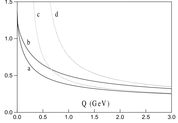
Figure 1: The bundle of analytic solutions. The curves (a) and (b) are the 1-loop analytic $\bar{\alpha}_{s}$ for $\Lambda=$200 MeV and 400 MeV, respectively; the curves (c) and (d) show the corresponding perturbative result.

Another important virtue of Eq. (5) is that the analytic behavior in the IR domain is provided by a nonperturbative contribution $\simeq\exp(-1/a\beta_{0})$.

To analyze the two-loop case, let us start with $\bar{a}^{(2)}(Q^{2})$ written down in the form

$$\bar{a}^{(2)}_{RG}(Q^{2})=\frac{1}{\beta_{0}l+\beta_{0}b_{1}\ln(1+l/b_{1})}~{},\quad l=\ln\frac{Q^{2}}{\Lambda^{2}}\,,$$ (6)

where $b_{1}=\beta_{1}/(\beta_{0})^{2}$ and $\beta_{1}=102-38/3n_{f}$ is the two-loop coefficient. This expression corresponds to the result of exact integration of the two-loop differential RG equation resolved by an iteration and generates a popular two-loop formula with $\ln l/l^{2}$ term.

For the spectral density, we get

$$\beta_{0}\rho^{(2)}_{RG}(L)\,=\,\frac{I(L)}{R^{2}(L)\,+\,I^{2}(L)}\,,\quad L=\ln\frac{\sigma}{\Lambda^{2}}$$ (7)

with

$$R(L) = L+b_{1}\ln\sqrt{\left(1+\frac{L}{b_{1}}\right)^{2}+\left(\frac{\pi}{b_{1}}\right)^{2}}~{},$$ (8)

$$I(L) = \pi+b_{1}{\rm arccos}\frac{b_{1}+L}{\sqrt{\left(b_{1}+L\right)^{2}+\pi^{2}}}~{}.$$

Now, to obtain $\bar{a}^{(2)}_{{\rm an}}(Q^{2})$, one has to substitute Eq. (7) into the r.h.s. of Eq. (2). However, the integral expression thus obtained is too complicated for presenting in an explicit form as the integration result differs from the used input $\bar{a}^{(2)}_{RG}$ not only by the pole term “subtracting” the ghost pole (as in the one-loop case), but also by an integral along the unphysical cut $~{}~{}0<Q^{2}<\Lambda^{2}\exp(-b_{1})~{}~{}$ “born” by the log-of-log dependence. For a quantitative discussion we have to use numerical calculation.

Nevertheless, for a particular value at $Q^{2}=0$ we can make two important statements. First, the IR limiting coupling value $\bar{\alpha}_{{\rm an}}(0)\,$, generally, does not depend on the scale parameter $\Lambda$. This is a consequence of RG invariance (compare with Ref.[5]) and in our case follows directly from Eq.(4). Second, the IR limiting coupling value is defined by the one-loop approximation, that is in the two-loop case coincides with the one-loop case: $\bar{\alpha}_{{\rm an}}^{(2)}(0)\,=\,\bar{\alpha}_{{\rm an}}^{(1)}(0)\,\equiv\bar{\alpha}_{{\rm an}}(0)$.

To obtain a simple proof for the two-loop case, it is convenient to express the difference $\bar{\alpha}_{{\rm an}}^{(1)}(0)-\bar{\alpha}_{{\rm an}}^{(2)}(0)$ via the imaginary part of the integral

$$\Delta\,=\,\int_{C}\,\frac{dz}{z}\,\frac{\ln(1\,+\,z)}{z\,+\,\ln(1\,+\,z)}$$ (9)

with the contour $C$ defined by $-\infty<{\rm Re}z<+\infty,\,{\rm Im}z=-\pi/b_{1}$. As far as the integrand is an analytic function in the half-plane below the contour C, we conclude that $\Delta=0$. Note also that the universality of $\bar{a}_{{\rm an}}(0)$ follows directly from the procedure of constructing the analytic coupling. Indeed, our two-loop input Eq. (6) has the ghost pole at $Q^{2}=\Lambda^{2}$ and the unphysical cut mentioned above. The analytization procedure removes these parasitic singularities by two compensation terms. The term that removes the pole gives the contribution $\Delta\bar{a}(0)_{{\rm pole}}=1/(2\beta_{0})$. The second term that compensates the cut can be expressed via the discontinuity of function (6) on this cut and presented as

$$\Delta\bar{a}(0)_{{\rm cut}}\,=\,\frac{1}{\beta_{0}}\,\int_{0}^{\infty}\,\frac{dz}{(z+1-\ln\,z)^{2}\,+\,\pi^{2}}\,,$$ (10)

which equals $1/(2\beta_{0})$ and we again obtain the universal value of $\bar{a}_{{\rm an}}(0)=1/\beta_{0}$. Thus, in contrast to perturbation theory, where the many-loop corrections change the IR behavior of the running coupling significantly, our analytic coupling has a stable IR limit. The analytization procedure removing all unphysical singularities leaves us with the physical cut which is mainly described by the one-loop contribution.

Note also that the universality of the value of $\bar{a}_{{\rm an}}(0)$ is not simply a matter of approximate resolution, Eq. (6), of the exact RG solution – it has a deeper ground. This fact can be established in a more general context, e.g., by considering the analytic properties, given by the analytization prescription, in the complex $1/a$-plane. The details of this reasoning are rather lengthy and will be published elsewhere.

Thus, the $\bar{\alpha}_{{\rm an}}(0)$ value, due to the RG invariance, is independent of $\Lambda$ and, due to the analytic properties, independent of higher corrections. This means that the causality (=analyticity) property brings the feature of the universality.

Here, we mean also that the whole shape of the $\bar{\alpha}_{{\rm an}}(Q^{2})$ evolution turns out to be reasonably stable with respect to higher corrections. The point is that the universality of $\bar{\alpha}_{{\rm an}}(0)$ practically gives rise to stability of the ${\bar{\alpha}_{{\rm an}}^{(\ell)}(Q^{2})}$ behavior with respect to higher correction in the whole IR region. On the other hand, this stability in the UV domain is a reflection of the property of asymptotic freedom. As a result, our analytic model obeys approximate “higher loops stability” in the whole Euclidean region. Numerical calculation (performed in the $\overline{{\rm MS}}$ scheme for one-, two-, and three-loop cases with $n_{f}=3$) reveals that ${\bar{\alpha}_{{\rm an}}^{(2)}(Q^{2})}$ differs from ${\bar{\alpha}_{{\rm an}}^{(1)}(Q^{2})}$ within the 10% interval and ${\bar{\alpha}_{{\rm an}}^{(3)}(Q^{2})}$ from ${\bar{\alpha}_{{\rm an}}^{(2)}(Q^{2})}$ within the 1% limit. This fact is demonstrated in Fig. 2

 

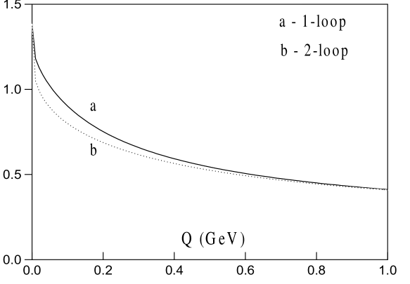
Figure 2: “Higher loop stability” of the analytic solution. The normalization point is on the $\tau$ lepton scale: $\bar{\alpha}_{s}(M_{\tau}^{2})=$0.34. Practically, the curve ${\bar{\alpha}_{{\rm an}}^{(3)}(Q^{2})}$ coincides with ${\bar{\alpha}_{{\rm an}}^{(2)}(Q^{2})}$ and we do not plot it in the figure.

It seems that the IR stability is an intrinsic feature of a non-analytic (in $\alpha_{s}$) contribution. To illustrate this thesis, consider a recent IR modification, ${\bar{\alpha}_{B}(Q^{2})}$, for the QCD running coupling by Badalian and Simonov [6]. These authors have studied a non-perturbative contribution to the QCD running coupling on the basis of the general background formalism using nonperturbative background correlators as a dynamic input. They came to the conclusion that these effects can practically be described by introducing an effective gluonic mass $M_{B}=\sqrt{2\pi\sigma}$ defined by string tension $\sigma$ into all “gluonic logarithms”: $\ln Q^{2}\to\ln(Q^{2}+M_{B}^{2})$. This means that ${\bar{\alpha}(Q^{2})}$ essentially slows down its evolution (i.e., freezes) around $Q\simeq M_{B}$. Their numerical estimate gave $M_{B}\simeq 1.5~{}{\rm GeV}$. In practice, this yields the difference between one– and two–loop results in the IR region of $15\%$ order.

In our calculations, we used $n_{f}=3$ as an average quark number. This seems to be reasonable in the low energy region $Q<2\,{\rm GeV}\simeq m_{c}$. For a more realistic description of the $\bar{\alpha}_{s}(Q)$ evolution in the whole Euclidean domain, one should take into account quark thresholds. To this end, one usually applies a matching procedure, changing abruptly the number of active quarks at an “effective” threshold $Q=\xi m_{q}$ with some matching parameter $\xi\simeq 1$. Evidently, any procedure of that sort violates the $Q^{2}$ analytic properties. On the other hand, these properties could be preserved by the “smooth matching” algorithm devised [7] on the base of an explicitly mass-dependent RG formalism ascending to Bogoliubov. This algorithm has been recently used [8] for the precise analysis of the $\bar{\alpha}_{s}(Q)$ evolution in the $3\,{\rm GeV}<Q<100\,{\rm GeV}$ interval.

In the present context it could be applied also in the $Q\leq\Lambda$ domain. However, this would change the $\bar{\alpha}_{{\rm an}}(Q^{2})$ behavior in the “very low $Q$” region only slightly as far as the limiting $\bar{\alpha}_{{\rm an}}(0)$ value depends on $\beta_{0}(n_{f}^{*})$ with the effective quark number $n_{f}^{*}$ related to the ghost-pole position $\Lambda$. As it is generally accepted on the base of DIS data, in the $\overline{{\rm MS}}$ scheme $\Lambda_{n_{f}=3}(2-{\rm loop})\simeq 250\div 350\,{\rm MeV}$ which is quite above of the strange quark mass. This means that the use of value $n_{f}^{*}=3$ is justified.

Analytic properties of the running coupling are important from the point of view of phynomenological applications, for example, for the description of the inclusive decay of the $\tau$ lepton. To this end, one usually transforms the initial expression for the $R_{\tau}$ ratio to the integral form in the complex $q^{2}$-plane (see, e.g., [9]). This transformation based on analytic properties mentioned above which are violated in the standard perturbative consideration and maintained within our method. Note also that referring to “low-$Q$” data, like those of $\tau$-lepton decay, one should distinguish between QCD scale $\Lambda^{\overline{{\rm MS}}}$ in the usual RG solution taken in the $\overline{{\rm MS}}$ scheme and $\Lambda^{{\rm an}}$ corresponding to our analytic expression. For instance, in the one-loop case, to the $\bar{\alpha}_{s}(M_{\tau}^{2})=0.34$ there correspond $\Lambda_{3}^{{\rm an}}=280\,{\rm MeV}$ as compared with $\Lambda_{3}^{\overline{{\rm MS}}}=230\,{\rm MeV}$.

The idea that the QCD running coupling can be frozen or finite at small momenta has been considered in many papers (see, e.g., the discussion in [10]). There seems to be experimental evidence in favor of this behavior of the QCD coupling in the IR region. As an appropriate object for comparison with our construction, we use the average

$$A(Q)\,=\,\frac{1}{Q}\,\int_{0}^{Q}\,dk\,{\bar{\alpha}_{s}}(k^{2})$$ (11)

that people manage to extract from jet physics data. Empirically, it has been claimed that this integral at $Q\simeq 1\div 2$ GeV turns out to be a fit-invariant quantity. For it there is an estimate: $A(2\,\,{\rm GeV})=0.52\pm 0.10$ [11]. Our results for $A(2\,\,{\rm GeV})$ obtained by the substitution $\bar{\alpha}^{(1)}_{{\rm an}}$ and $\bar{\alpha}^{(2)}_{{\rm an}}$ into Eq. (11) for some values of the running coupling at the normalization point $\mu^{2}=M_{\tau}^{2}$ are summarized in the Table.

$\bar{\alpha}_{{\rm an}}(M_{\tau}^{2})$	0.34	0.36	0.38
$A_{{\rm 1-loop}}(2\,{\rm GeV})$	0.50	0.52	0.55
$A_{{\rm 2-loop}}(2\,{\rm GeV})$	0.48	0.50	0.52

Note here that a nonperturbative contribution, like the second term on the l.h.s. of Eq. (5), reveals itself even at moderate $Q$ values by “slowing down” the rate of $\bar{\alpha}_{s}(Q)$ evolution. For instance, in the vicinity of the $c$ and $b$ quark thresholds at $Q=3\,{\rm GeV}$ it contributes about 4%, which could be essential for the resolution of the “discrepancy” between “low-$Q$” data and direct $Z_{0}$ measurement for $\bar{\alpha}_{s}(M_{Z})$.

In this letter, we have argued that a possible way to resolve the ghost-pole problem for the QCD running coupling can be found by imposing the Käll$\acute{{\rm e}}$n-Lehmann $Q^{2}$-analyticity which reflects the causality principle of QFT. The analytic behavior in the IR region is restored by a nonperturbative contribution. The procedure of constructing the analytic running coupling is not unambiguous [12]. We have considered the simplest way which does not require any additional parameters and operates only with $\Lambda$ or a value of the coupling at a certain normalization point. The requirement of analyticity yields significant modification in the IR and intermediate domains and leads to the universal value of $\bar{\alpha}_{{\rm an}}(0)$. In this paper we have obtained the analytically-improved result $\bar{\alpha}_{{\rm an}}(Q^{2})$ for the QCD running coupling that turns out to be quite stable with respect to higher-order corrections for the whole interval of $Q^{2}$ and agrees with low energy experimental evidence for the IR-finite behavior.

Our construction does not contain adjustable parameters. This is due, in particular, to the convergence of a nonsubtracted spectral integral, that is, with the asymptotic freedom property. Here, analyticity plays the role of a bridge between regions of small and large momenta. The idea that “analyticity is the key factor relating high energy to low energy” has recently been emphasized by Nishijima [13] in the context of connection between the asymptotic freedom and color confinement. However, in our approach this connection is not so direct. If, e.g., we admit (see Ref. [14]) the possibility of a UV fixed point for the QCD effective coupling at some small value of $\alpha_{s}\leq 0.05$, then we arrive at a modification of the UV behavior with a power instead of $(\ln\sigma)^{-2}$ decrease of the spectral function. So, in that case we can also use a nonsubtracted spectral representation.

As far as it is difficult to present an explicit analytic expression for ${\bar{\alpha}_{{\rm an}}^{(2)}(Q^{2})}$, for the need of QCD practitioners, we propose an approximate formula. It can be obtained by the method of subtraction of unphysical singularities if one takes into account the explicit expression for the term that removes the ghost pole and an approximate expression in the form of the first term of the power expansion for the term that removes the unphysical cut. The corresponding expression reads

$$\beta_{0}\tilde{a}^{(2)}(Q^{2})\simeq\beta_{0}\bar{a}^{(2)}_{RG}(Q^{2})+\frac{1}{2}\;\frac{1}{1-Q^{2}/\Lambda^{2}}-\frac{\Lambda^{2}}{Q^{2}}C_{1}\,,$$ (12)

where $\bar{a}^{(2)}_{RG}(Q^{2})$ is defined by (6) and, for $n_{f}=3$, $C_{1}=0.035$. Expression (12) approximates the two-loop analytic coupling with an accuracy less than 0.5% in the region $2.5\,\Lambda<Q<3.5\,\Lambda$, practically coincides with the exact formula for larger values of momenta, and, therefore, can be used in the analysis of many experimental data. If there is necessary to consider a very small momentum, like Eq. (11), we suggest another approximate formula which can be written in the form of Eq. (5) with substitution, instead $Q^{2}/\Lambda^{2}$, the expression $\exp[\ln\,{Q^{2}}/{\Lambda^{2}}+b_{1}\ln\sqrt{\ln^{2}\,{Q^{2}}/{\Lambda^{2}}+4\pi^{2}}].$ For $Q\geq\Lambda$, the accuracy of this approximation is less than 5% and yields only 3% error into the $A(2\,{\rm GeV})$ value.

The authors would like to thank A.M. Baldin, H.F. Jones, A.L. Kataev, K.A. Milton, V.A. Rubakov and O.P. Solovtsova for interest in the work and useful comments. Partial support of D.Sh. by INTAS 93-1180 and RFBR 96-15-96030 grants and of I.S. by the US NSF grant PHY-9600421 is gratefully acknowledged.

References

- [1] P. Redmond, Phys. Rev. 112 1404 (1958); P. Redmond and J.L. Uretsky, Phys. Rev. Lett. 1 147 (1958).
- [2] N.N. Bogoliubov, A.A. Logunov and D.V. Shirkov, Sov. Phys. JETP 37(10) 574 (1960).
- [3] D.V. Shirkov and I.L. Solovtsov, JINR Rapid Comm., No. 2[76]-96, 5, hep-ph/9604363.
- [4] I.F. Ginzburg and D.V. Shirkov, Sov. Phys. JETP 22 234 (1966).
- [5] M. Gell-Mann and F. Low, Phys.Rev., 95 1300 (1954).
- [6] Yu.A. Simonov, Yad. Fizika, 58 1139 (1995); A.M. Badalian and Yu.A. Simonov, loc. cit. (to be published).
- [7] D.V. Shirkov, Nucl. Phys. B 371 476 (1992).
- [8] D.V. Shirkov and S.V. Mikhailov, Z. Phys. C 63 463 (1994).
- [9] E. Braaten, S. Narison and A. Pich, Nucl. Phys. B 373 581 (1992).
- [10] A.C. Mattingly and P.M. Stevenson, Phys. Rev. D 49 437 (1994).
- [11] Yu.L. Dokshitzer and B.R. Webber, Phys. Lett. B 352 451 (1995); Yu.L. Dokshitzer, V.A. Khoze and S.I. Troyan, Phys. Rev. D 53 89 (1996).
- [12] D.A. Kirzhnits, V.Ya. Fainberg and E.S. Fradkin, Sov. Phys. JETP 11 174 (1960).
- [13] K. Nishijima, Czech. J. Phys. 46 1 (1996).
- [14] A. Patrascioiu and E. Seiler, Phys. Rev. Lett. 74 1920 (1995); ibid 74 1924 (1995).