Multiple inflation

Abstract

Attempts at building an unified description of the strong, weak and electromagnetic interactions usually involve several stages of spontaneous symmetry breaking. We consider the effects of such symmetry breaking during an era of primordial inflation in supergravity models. In cases that these occur along flat directions at intermediate scales there will be a succession of short bursts of inflation which leave a distinctive signature in the spectrum of the generated scalar density perturbation. Thus measurements of the spectral index can directly probe the structure of unified theories at very high energy scales. An observed feature in the power spectrum of galaxy clustering from the APM survey may well be associated with such structure. If so, this implies a characteristic suppression of the secondary Doppler peaks in the angular power spectrum of temperature fluctuations in the cosmic microwave background.

I Introduction

Cosmological inflation is an attractive idea in search of a basis in physics beyond the Standard Model [1]. It has become increasingly clear over the past decade that the most compelling such extension of physics is the local version of supersymmetry (SUSY), i.e. supergravity (SUGRA) [2]. This provides a natural framework for obtaining the required extremely flat and radiatively stable potential for the scalar ‘inflaton’ field $\phi$, the large and approximately constant vacuum energy of which drives an exponential increase of the scale-factor and is then converted to radiation when the inflaton settles into its global minimum [3, 4]. There has also been impressive progress in astronomical observations of large-scale structure (LSS) in the universe [5] and of angular anisotropy in the cosmic microwave background (CMB) [6], which provide detailed constraints on the spectrum of quantum fluctuations generated during the inflationary De Sitter era, and therefore on the inflaton potential [7]. Together these advances promise to shed light on the structure of the theory at very high energies for it is known [1, 7] that the amplitude of the large angular scale CMB fluctuations observed by COBE require the energy scale $\Lambda$ of the responsible inflationary era to be well above the electroweak scale. We refer to this era as ‘primordial inflation’.

Most SUGRA models of inflation studied so far contain the inflationary potential in a sector termed ‘hidden’ because it is coupled only gravitationally to the visible sector containing the quarks and leptons and the states responsible for their non-gravitational interactions. This is done because the required flatness of the inflaton potential is easily maintained in the hidden sector. In such schemes, the physics of the visible world appears to play no significant role during inflation. In this paper we will demonstrate that this is not necessarily the case because the visible sector may undergo spontaneous symmetry breaking during inflation. This can have significant effects on the quantum fluctuations of the inflaton through the inevitable gravitational interactions.

There are two essential requirements for this to have observationally interesting effects. The phase transition should occur during inflation and the subsequent amount of inflation should be small enough so as not to inflate the density perturbation generated during the phase transition to scales beyond the present horizon. Both conditions are naturally met in supergravity models.

To see this, let us consider the origin of symmetry breaking in supergravity theories. We view these as the effective “low-energy” theories originating from the underlying unified ‘Theory of Everything’, the only viable candidate for which is the superstring. In the latter, the fundamental scale is the string tension which may be re-interpreted as the Planck scale; all other scales must be generated by spontaneous symmetry breakdown. How does this occur? The first requirement is a source of SUSY breaking. The origin of this is not firmly established but the most promising mechanism is through a stage of dynamical symmetry breaking involving a strongly coupled hidden sector. In analogy with QCD it is then reasonable to assume that the strongly interacting fermions — the gaugino partners of the gauge boson of the strong group — form a condensate which necessarily breaks local SUSY. The scale of SUSY breaking is the scale at which the coupling becomes strong and thus, like QCD, can be far from the Planck scale. Once SUSY is broken, this breaking is communicated to all sectors of the theory via gravitational interactions.

For our present purposes all we need to assume is some mechanism that gives such an initial source of ‘soft’ SUSY breaking mass terms for all the fields of the theory. The scale for these is set by the gravitino mass $m_{3/2}$, which must be of ${\cal O}(m_{W})$ if the hierarchy problem is to be solved allowing for a small electroweak breaking scale. Now consider the possible sources of gauge symmetry breaking. In supersymmetric theories there are many ‘flat’ directions, even amongst fields with large gauge (or other) couplings. These are directions in field space along which, in the absence of SUSY breaking, the potential identically vanishes or occurs only in higher order, suppressed by some power of the Planck scale. Along such directions, which we will characterize by the field $\rho$, the SUSY breaking mass terms will be the dominant terms in the potential. If the mass-squared is negative at the origin of field space, symmetry breaking occurs along the flat direction and the vacuum expectation value (vev) of $\rho$, which we denote by $\Sigma$, will be determined by the stabilizing higher order terms. Since these are small, the vev $\Sigma$ will be very large and can be close to the Planck scale. The important point is that the SUSY breaking trigger for fields in the visible sector is small, of ${\cal O}(m_{3/2})$. This is true even though the scale of symmetry breaking thus generated is very large. It is now easy to see why such a stage of symmetry breaking in the visible sector must necessarily occur during primordial inflation. The reason is that the gauge and/or Yukawa interactions of the field $\rho$ will ensure that it is in thermal equilibrium before inflation. Thus there will be stabilizing terms $\propto\,\rho^{2}T^{2}$ in the full effective potential $V(\phi,\rho,T)$ which will prevent the transition to the asymmetric minimum from occurring until the temperature drops to $T\sim\,m_{3/2}$. This happens only after several e-folds of inflation as we shall demonstrate. Thereafter the phase transition will occur but this will affect the inflaton sector only through gravitational corrections. If these are small, inflation will continue.

Thus we have the first ingredient necessary for imprinting structure onto the (nearly) scale-invariant scalar density perturbation generated during inflation because, as the phase transition occurs, the mass of the inflaton changes through its gravitational coupling to $\rho$. This would be irrelevant if inflation continues afterwards for more than about $50$ e-folds for then any such structure would then be inflated to spatial scales larger than our present horizon. However this may not happen if there is more than one stage of intermediate scale symmetry breaking. Then there will be several phase transitions in succession each of which imprints structure on the density perturbation. At each stage there is the possibility that the gravitational coupling of the inflaton to the visible sector may change the inflaton potential to such an extent that it causes inflation to end. This provides the second essential ingredient in that it makes it likely that the structure in the density perturbation produced during the previous phase transitions will be inflated by a limited number of e-folds and thus may still remain within our observable horizon.

This is not yet the end of the story because on reheating after inflation, the symmetries in the visible sector may be restored by thermal effects. Thus as the universe cools during the radiation-dominated era, the field $\rho$ may again be trapped at the origin until the temperature drops below $T\sim\,m_{3/2}$. Now the potential energy in the visible sector will dominate and generate a late era of inflation. When this behaviour was first noticed a decade ago [8, 9] it was considered to be an “entropy crisis” since it would erase the baryon asymmetry presumed to have been generated at the GUT scale. We know now that there are several plausible mechanisms for low temperature baryogenesis well below the GUT scale, for example electroweak baryogenesis [10] as well as the Affleck-Dine mechanism which is specific to the flat directions under discussion [11]. Therefore late inflation is no longer a fatal problem. Indeed the above mechanism has recently been revived [12] under the name ‘thermal inflation’ to offer a plausible solution to the problem of overproduction (after primordial inflation) of moduli fields with electroweak scale (or heavier) masses. Again the crucial observation is that only a limited number of e-folds of inflation occur, so such late inflation [13] does not destroy the success of primordial inflation in providing the density perturbation responsible for the CMB anisotropy observed by COBE and necessary to seed the growth of the observed large-scale structure.

With this motivation we now turn to a quantitative study of such multiple inflation in supergravity models. A preliminary account of this work was presented earlier [14].

II The scalar potential in supergravity

In this section we review the form of a $N=1$ supergravity potential. The results of relevance to the inflationary potential will be summarised in the next section so the reader not interested in the fine details may skip this section.

In constructing a model of inflation we are interested in the form of the potential for the scalar ‘inflaton’ field, viz. the order parameter associated with a phase transformation which generates a period of exponentially fast growth of the cosmological scale parameter. In $N=1$ supersymmetric theories with a single SUSY generator, complex scalar fields are the lowest components, $\phi^{a}$, of chiral superfields, $\Phi^{a}$, which contain chiral fermions, $\psi^{a}$, as their other components. In what follows we will take $\Phi^{a}$ to be left-handed chiral superfields so that $\psi^{a}$ are left-handed massless fermions. Masses for fields will be generated by spontaneous symmetry breakdown so that the only fundamental mass scale is the normalized Planck scale, $M\equiv\,M_{\rm P}/\sqrt{8\pi}\simeq 2.44\times 10^{18}$ GeV. This is aesthetically attractive and is also what follows if the underlying theory generating the effective low-energy supergravity theory follows from the superstring. The $N=1$ supergravity theory describing the interaction of the chiral superfields is specified by the Kähler potential [2],

$$G(\Phi,\Phi^{\dagger})=d(\Phi,\Phi^{\dagger})+\ln|f(\Phi)|^{2}.$$ (1)

Here $d$ and $f$ (the superpotential) are two functions needed to specify the theory; they must be chosen to be invariant under the symmetries of the theory. The dimension of $d$ is 2 and that of $f$ is 3, so terms bilinear (trilinear) in the superfields appear without any mass factors in $d$ ($f$). The scalar potential following from eq.(1) is given by [2]

$$V=\exp\left(\frac{d}{M^{2}}\right)\left[F^{A^{\dagger}}(d_{A}^{B})^{-1}F_{B}-3\frac{|f|^{2}}{M^{2}}\right]+{\rm D-terms}\ ,$$ (2)

where

$$F_{A}\equiv\frac{\partial f}{\partial\Phi^{A}}+\left(\frac{\partial d}{\partial\Phi^{A}}\right)\frac{f}{M^{2}}\ ,\qquad\left(d_{A}^{B}\right)^{-1}\equiv\left(\frac{\partial^{2}d}{\partial\Phi^{A}\partial\Phi_{B}^{\dagger}}\right)^{-1}.$$ (3)

We follow ref.[15] in expanding $f$ and $d$ as a series in $M$

$$f(z,y) = M^{2}f^{(2)}(\frac{z}{M})+Mf^{(1)}(\frac{z}{M})+f^{(0)}(\frac{z}{M},y)\ ,$$ (4)

$$d(z,z^{\dagger},y,y^{\dagger}) = M^{2}d^{(2)}(\frac{z}{M},\frac{z^{\dagger}}{M})+Md^{(1)}(\frac{z}{M},\frac{z^{\dagger}}{M})+d^{(0)}(\frac{z}{M},\frac{z^{\dagger}}{M},y,y^{\dagger})\ .$$ (5)

Here $z$ are chiral superfields whose scalar component have large vevs and $y$ correspond to those fields which do not have large vevs and which remain light. Thus the superfields $y$ cannot appear multiplied by powers of $M$, hence the form of eq.(5).

If, as is the case in theories descending from the superstring, there are no mass scales other than $M$ and those induced by spontaneous breaking, we have for the terms generating the renormalizable self couplings of the light fields $y$ the form [16]

$$f^{(0)}(\frac{z}{M},y) = \sum_{n}c_{n}(z)g_{n}^{(3)}(y)\ ,$$ (6)

$$d^{(0)}(\frac{z}{M},\frac{z^{\dagger}}{M},y,y^{\dagger}) = y^{a}\Lambda_{a}^{b}(\frac{z}{M},\frac{z^{\dagger}}{M})y_{b}^{\dagger}+\sum_{m}c^{\prime}_{m}(\frac{z}{M},\frac{z^{\dagger}}{M})g_{m}^{(2)}(y)+{\rm h.c.}\ ,$$ (7)

where $g_{n}^{(3)}(y)$ and $g_{m}^{(2)}(y)$ are, respectively, the trilinear and bilinear terms in $y^{a}$ allowed by the symmetries of the theory. In addition there will be further terms in eq.(7) suppressed by inverse powers of $M$ which generate non-renormalizable terms involving the light fields $y$ in the effective low energy Lagrangian.

From ref.[16], the terms in the effective potential which survive in the $M\rightarrow\infty$ limit (keeping terms of order $z/M$) are:

$$V \approx \left|\frac{\partial\hat{g}}{\partial y^{a}}\right|^{2}+m_{3/2}^{2}y^{a}S_{a}^{b}y_{b}^{\dagger}+[m_{3/2}^{\dagger}(y^{a}R_{a}^{b}\frac{\partial\hat{g}}{\partial y^{b}}+\sum_{n}(A_{n}-3)\hat{g}^{(3)}_{n}$$ (9)

$$+\sum_{n}(B_{m}-2)\mu_{m}g_{m}^{(2)})+{\rm h.c.}]+{\rm D-terms}\ ,$$

where

$$m_{3/2}\equiv\langle{\rm e}^{d^{(2)}/2}f^{(2)}\rangle$$ (10)

is the gravitino mass, and

$$S_{a}^{b}=\delta^{b}_{a}+M^{2}\left\langle\rho^{\dagger i}\left(\frac{\partial\Lambda_{c}^{b}}{\partial z^{\dagger}_{j}}\frac{\partial\Lambda_{a}^{c}}{\partial z^{i}}-\frac{\partial^{2}\Lambda_{a}^{b}}{\partial z^{\dagger}_{j}\partial z^{i}}\right)\rho_{j}\right\rangle,\qquad R_{a}^{b}=\delta_{a}^{b}-M\left\langle\rho^{\dagger i}\frac{\partial\Lambda_{a}^{b}}{\partial z^{i}}\right\rangle,$$ (11)

where

$$\rho_{j}\equiv\left(M\frac{\partial^{2}d^{(2)}}{\partial z^{i}\partial z^{\dagger}_{j}}\right)^{-1}\frac{\partial}{\partial z^{j}}(\ln f^{(2)}+d^{(2)})\ .$$ (12)

Here $\hat{g}$ is the superpotential for the light fields defined by

$$\hat{g}(y)=\sum_{n}\hat{g}^{(3)}_{n}(y)+\sum_{m}\mu_{m}g_{m}^{(2)}(y)\ ,$$ (13)

with

$$\hat{g}^{(3)}_{n}(y)=\langle{\rm e}^{d^{(2)}/2}S\rangle c_{n}(\langle{\frac{z}{M}}\rangle)g_{n}^{(3)}(y)\ ,\qquad\mu_{m}=m_{3/2}\left\langle\left(1-M\rho_{i}\frac{\partial}{\partial z^{\dagger}_{i}}\right)c_{m}^{\prime}({\frac{z}{M}},{\frac{z^{\dagger}}{M}})\right\rangle.$$ (14)

The coefficients $A_{n}$ and $B_{m}$ are given by

$$A_{n} = M\left\langle\rho^{\dagger i}\frac{\partial}{\partial z^{i}}[d^{(2)}+\ln c_{n}(\frac{z}{M})]\right\rangle,$$ (15)

$$B_{m} = \left\langle\left[2+M\left(\rho^{\dagger i}\frac{\partial}{\partial z^{i}}-\rho_{i}\frac{\partial}{\partial z^{\dagger}_{j}}\right)-M^{2}\rho^{\dagger i}\rho_{j}\frac{\partial^{2}}{\partial z^{i}\partial z^{\dagger}_{j}}\right]\frac{c^{\prime}_{m}(\frac{z}{M},\frac{z^{\dagger}}{M})}{(1-M\rho_{i}\frac{\partial}{\partial z^{\dagger}_{i}}c^{\prime}_{m}(\frac{z}{M},\frac{z^{\dagger}}{M})}\right\rangle.$$ (16)

A Constraints on the inflaton potential

The question whether the form of eq.(9) is such as to generate a period of inflation has been considered extensively in the literature [4]. For our purposes here it is sufficient to introduce a general formalism encompassing the various possibilities by expanding the (slowly varying) potential about the value $\phi^{*}$ in inflaton field space at which the quantum fluctuations of interest are produced. Thus we write $\phi=\tilde{\phi}+\phi^{*}$ (in units of $M$) and expand the inflaton potential as

$$V_{\rm I}(\phi)=\Lambda^{4}\left[1+c_{1}\tilde{\phi}+c_{2}\tilde{\phi}^{2}+c_{3}\tilde{\phi}^{3}+c_{4}\tilde{\phi}^{4}+\dots\right]\ .$$ (17)

Here we have factored out the overall scale of inflation $\Lambda$ which is usually required to be $\sim 10^{-4}M$ in order to account for the CMB anisotropy observed by COBE [17, 18]. Note that since a non-zero potential breaks supersymmetry, the magnitude of SUSY breaking during inflation is different from that after inflation. During inflation the gravitino mass receives a contribution of order the Hubble parameter [19] which, in this case, is

$$|m_{3/2}|\sim\frac{\Lambda^{2}}{M}\sim 10^{-8}M\ ,$$ (18)

i.e. much larger than its nominal value of ${\cal O}(m_{W})$.

The constraints on the parameters in the potential following from the ‘slow-roll’ conditions [7] for successful inflation are

$$c_{1}\ll 1\ ,\quad c_{2}\ll 1\ ,\quad c_{3}\tilde{\phi}\ll 1\ ,\quad c_{4}\tilde{\phi}^{2}\ll 1\ ,\ \ldots$$ (19)

We focus on ‘new inflation’ in which initially $\tilde{\phi}\ll\,1$, so the constraints are only severe for $c_{1}$ and $c_{2}$. A variety of models have been examined in which these constraints are automatically satisfied [4]. For example symmetry may give $c_{1},~{}c_{2}=0$ while $c_{3}$ and $c_{4}$ are of ${\cal O}(1)$ [17, 18]. More interestingly, the problematic quadratic term may dynamically relax to zero by virtue of an infrared fixed point at the origin for the coupled equations of motion of the inflaton field $\tilde{\phi}$ and the modulus field $\varphi$ which determines its couplings [20]. This requires only that the kinetic term have a symmetry leading to (pseudo) Goldstone modes and the resulting scalar potential then has the form (17) with the coefficients

$$c_{1}=0\ ,\quad c_{2}\sim\varphi\ ,\quad c_{3}\sim 1\ ,\quad c_{4}\sim 1\ ,\ \ldots$$ (20)

The fields are driven to the initial values $\varphi,|\tilde{\phi}|\sim\,H$ so the ‘quadratic’ and cubic terms become comparable; thereafter $\tilde{\phi}$ grows more rapidly than $\varphi$ and the cubic term soon dominates [20]. This results in a ‘tilted’ spectrum for the scalar density perturbation which solves the problem of excess power on small spatial scales in the COBE-normalized cold dark matter (CDM) cosmogony.

For the present discussion, the precise form chosen is not crucial, so we proceed under the assumption that there is a hidden sector inflationary potential satisfying the slow-roll conditions.

III Multiple primordial inflation

As discussed above, supersymmetric theories may have ‘flat’ directions in field space along which combinations of fields may acquire vevs without changing the potential significantly. Gauge singlet moduli fields of the type found in superstrings [21] provide an example of this, having absolutely flat potentials in the absence of SUSY breaking. The same may be true for strongly interacting fields e.g. gauge non-singlets may acquire vevs along ‘D-flat’ directions. Along these flat directions it is the SUSY breaking masses that determine the vevs. For example, if the potential for a field $y$ is completely flat in the absence of SUSY breaking, the superpotential $f$ in eq.(1) vanishes identically and the scalar potential is given by eq.(9) as

$$V\approx m_{3/2}^{2}(S|y|^{2}+Ty^{2}+{\rm h.c.})\ ,$$ (21)

where

$$S_{b}^{a}=S\delta_{b}^{a}\ ,\qquad T=(B_{m}-2+2R)\left\langle\left(1-M\rho_{i}\frac{\partial}{\partial z_{i}^{\dagger}}\right)c_{m}^{\prime}({\frac{z}{M}},\frac{z^{\dagger}}{M})\right\rangle\frac{\partial^{2}g_{m}^{(2)}}{\partial y^{2}}\ ,\qquad R_{b}^{a}=R\delta_{b}^{a}\ .$$ (22)

We see that the scalar potential is proportional to the square of the SUSY breaking parameter $m_{3/2}$, thus vanishing in the supersymmetric limit.

Let us now consider the potential for a field $\rho$ which triggers a stage of symmetry breaking in the visible sector (for simplicity $\rho$ may be taken to be real). The full scalar potential describing the inflaton field $\phi$ and the visible sector field $\rho$ is

$$V=V_{\rm I}(\phi)+m^{2}(\frac{\rho}{M})\ \rho^{2}[1+{\cal O}(\frac{\rho}{M})]\ .$$ (23)

Here we have allowed for the effect of radiative corrections in the visible sector which cause the SUSY breaking mass $m$ to run, with corrections dependent on the logarithm of $\rho/M$. If $m^{2}$ is positive at the Planck scale but changes sign due to these radiative corrections at a scale $\Sigma$, the potential will have a minimum at an ‘intermediate’ scale very close to $\Sigma$. In the case the flat direction described by $\rho$ is only approximately flat, there will be additional terms in the potential proportional to $\rho^{N}/M^{N-4}$ which will provide a stable minimum even if the SUSY breaking mass-squared is negative at the Planck scale. However even in this case the vev of the field $\rho$ at the minimum will be large, of ${\cal O}(M^{N-4}m_{3/2}^{2})^{1/(N-2)}$. Let us denote this scale too by $\Sigma$. For future reference we note that the depth of the potential in both cases is given approximately by $m_{3/2}^{2}\Sigma^{2}\sim\Lambda^{4}(\Sigma/M)^{2}$.

We are interested in the case $\rho$ is a visible sector field having strong (gauge and/or Yukawa) interactions which will maintain it initially in thermal equilibrium with a potential of the form [8]

$$V(\phi,\rho,T)=V_{\rm I}(\phi)+\left[-|m|^{2}(\frac{\rho}{M})+\alpha T^{2}\right]\rho^{2}[1+{\cal O}(\frac{\rho}{M})]\ .$$ (24)

where we have now explicitly indicated that $m^{2}$ is negative. This form applies for values of the $\rho$ field small enough that its mass is less than the temperature. Since $\rho$ has strong couplings this essentially requires $\rho<T$. Above this scale the thermal term in the effective potential above vanishes. Thus the thermal term creates a potential barrier of height $\sim\,T^{4}$ in between $\rho\sim\,T$ and $\rho\sim\,T^{2}/|m|$, which prevents the vev of $\rho$ from developing until the temperature drops to $T_{\rm f}\sim\,|m|\approx\,|m_{3/2}|$ and the barrier disappears [8, 22]. However, before this happens but after $T$ drops below $T_{\rm i}\sim\,V^{1/4}\approx\Lambda$, the approximately constant potential term $V_{\rm I}(\phi)$ dominates the thermal energy, driving a short period of inflation. Note that $T_{\rm f}$ is determined by the value of $m$ (given by eq.(18)) during this period of inflation, i.e. $T_{\rm f}\approx\,V_{\rm I}^{1/2}/M$. The important point is that the extent of this inflationary period is thus limited to $\ln(T_{\rm i}/T_{\rm f})\sim\ln(M/\Lambda)$ i.e. about 10 e-folds for $\Lambda\sim 10^{-4}M$. Subsequently the field $\rho$ evolves to its global minimum at $\Sigma$ according to the governing equation

$$\ddot{\rho}+3H\dot{\rho}+\frac{{\rm d}V}{{\rm d}\rho}=0\ ,$$ (25)

so its growth (for $\langle\rho\rangle\ll\Sigma$) obeys

$$\rho=\rho_{0}\exp\left[\frac{3Ht}{2}\left(\sqrt{1+\frac{8m^{2}}{9H^{2}}}-1\right)\right].$$ (26)

Since $|m|\sim\,H$ we have $\rho\sim\rho_{0}{\rm e}^{Ht}$ with $\rho_{0}\lesssim\,T_{\rm f}$, so there is a further $\sim\ln(\Sigma\,M/\Lambda^{2})$ e-folds of inflation before $\rho$ settles into its minimum and releases its stored energy. (However, because of the exponentially fast growth, most of the actual increase in $\langle\rho\rangle$ occurs in the last 1–2 e-folds.) Thus the total number of e-folds of inflation is:

$${\cal N}_{1}^{\rm prim}\sim\ln\left(\frac{\Sigma M^{2}}{\Lambda^{3}}\right).$$ (27)

As the intermediate scale transition occurs energy is released and there is the possibility of reheating in the visible sector to which $\rho$ is coupled. However fields strongly coupled to $\rho$ will obtain a large intermediate scale mass and thus will not be readily produced by $\rho$ decay or by its rescattering products. Thus one must consider only reheating processes to visible sector states $\chi$ which have coupling $h\rho^{2}\chi^{2}$ with the coupling constant $h$ constrained by $h\langle\rho\rangle<T_{\rm R}$, where $T_{\rm R}$ is the reheat temperature. With such a small coupling the energy release does not lead to reheating above the Hawking temperature $T_{\rm H}=H/2\pi$ in the De Sitter vacuum because of the large Hubble parameter during primordial inflation.

After the phase transition inflation continues but with a reduced scale, i.e.

$$V_{\rm I}\rightarrow V_{\rm I}\left[1-\left(\frac{\Sigma}{M}\right)^{2}\right].$$ (28)

This will have the effect of changing the amplitude of the generated density perturbation (see eq.(33)), albeit by a negligible amount for small $\Sigma/M$. A more significant change to the density perturbation will occur however due to the inevitable gravitational coupling between the $\rho$ and $\phi$ sectors, changing the inflaton mass. Note that since the latter is anomalously small relative to the Planck scale, small changes in it have a disproportionately large effect. The magnitude of this effect is easily estimated by adding to the effective low energy theory, terms allowed by the governing symmetries. Thus we may expect in eq.(1) a term $d\supset\beta\phi\phi^{\dagger}\rho^{2}/M^{2}$. Following from the scalar potential (2) this gives a contribution to the inflaton mass of

$$\delta m_{\phi}^{2}\sim m_{3/2}^{2}\ \beta\left(\frac{\Sigma}{M}\right)^{2},$$ (29)

to be compared with the effective inflaton mass during inflation given by eqs.(17) and (20),

$$m_{\phi}^{2}=m_{3/2}^{2}\ c_{3}\left(\frac{\langle|\tilde{\phi}|\rangle}{M}\right).$$ (30)

For $\beta(\Sigma/M)^{2}$ of ${\cal O}(c_{3}(\langle|\tilde{\phi}|\rangle/M))$, the inflatonary potential will be significantly modified and hence so too will be the density perturbation which is sensitive to the inflaton mass.

Of course if the second period of inflation continues for more than about $50$ e-folds the difference in the density perturbations produced in the two periods of inflation becomes observationally irrelevant. However, analyses of realistic models suggest there may be several flat directions and several stages of spontaneous symmetry breaking, so we may expect this new period of inflation to be short-lived as well because of a further stage of intermediate scale symmetry breaking (at a scale $\Sigma_{2}$) either running concurrently or triggered by the first stage of breaking (through the effect on the mass of the second ‘flat direction’ field of the vev of the first). This second period of inflation lasts just

$${\cal N}_{2}^{\rm prim}\approx\ln\left(\frac{\Sigma_{2}}{\Sigma}\right),\ \ln\left(\frac{\Sigma_{2}M}{\Lambda^{2}}\right)$$ (31)

e-folds for the two cases respectively. As before, after the second stage of breaking is completed, the form of the inflation potential may change significantly due to the gravitational coupling between the inflaton and ‘flat’ sectors. The whole process may continue for as many stages of intermediate scale breaking as there are flat directions.

What about the end of inflation? There are two possibilities. The first is that the end occurs in the usual manner when the inflaton vev becomes of ${\cal O}(M)$. Since the overall number of e-folds of inflation in a ‘slow-roll’ model is very large (see e.g. [18, 20]), one may expect that the total number of e-folds in the last period of inflation, after intermediate scale breaking, is also quite large, much greater than $50$, so the effect of the previous eras of intermediate scale breaking is observationally irrelevant. The second, more interesting, possibility is that at the end of one of the intermediate breaking stages the modification of the inflaton potential is so great that it ceases to satisfy the slow-roll conditions. As we have discussed (c.f. eq.(29)) this happens if $\beta(\Sigma_{i}/M)^{2}\sim 1$, for then the change in the $\phi$ potential violates eq.(19). In this case the corresponding intermediate scale phase transition ends inflation. Note that this may occur at any of the symmetry breaking stages since there is no requirement for the various intermediate scales $\Sigma_{i}$ to be all of the same magnitude. This follows because these depend sensitively on the form of the non-renormalizable higher dimension terms which lift the flatness of the potential in the supersymmetric limit.

When inflation is terminated, the potential energy $\Lambda^{4}$ of the inflaton $\phi$ is released. Reheating is inefficient in our model [17] as the inflaton has only gravitational couplings to the visible sector resulting in a slow decay rate $\Gamma_{\phi}\sim\Lambda^{6}/M^{5}$. As discussed earlier [18], the temperature at the beginning of the standard radiation dominated era is consequently low:

$$T_{\rm R}^{\rm prim}\sim\left(\sqrt{\frac{30}{\pi^{2}g_{\ast}}}\Gamma_{\phi}M\right)^{1/2}\sim 10^{5}\ {\rm GeV},$$ (32)

taking $g_{\ast}$, the effective number of relativistic degrees of freedom in the plasma, to be 915/4 as in the MSSM for $T\gg\,m_{W}$. There is no parametric resonance [23] since the inflaton has no coupling to the visible sector fields $\chi$ of the form $\phi^{2}\chi^{2}$ but only terms involving $\chi^{3}$ [18]. This is because the supergravity couplings involve the square of the superpotential $f$ which is trilinear in the scalar fields, therefore bilinear terms are suppressed by $m_{\chi}/M$. Note that even if the reheating were to be prompt due to an enhanced decay rate, energy conservation imposes the absolute bound

$$T_{\rm R}^{\rm prim}\sim\left(\sqrt{\frac{30}{\pi^{2}g_{\ast}}}HM\right)^{1/2}\lesssim\frac{\Lambda}{3}\ .$$

A The scalar density perturbation

The case inflation ends due to an intermediate scale transition after a series of such intermediate scale transitions implies a novel and interesting structure for the spectrum of the scalar density perturbation. In this picture our observational universe has resulted from a succession of inflationary periods, each lasting a relatively small number e-folds. The magnitude of the density perturbation during each period is determined by a combination of the parameters in the inflationary sector and in the intermediate scale sector. Thus we have a natural model for features in the perturbation spectrum which may be probed by observations of LSS and the CMB.

The magnitude of the density perturbation produced in a theory with multiple scalar fields has been discussed in ref.[24] following the formalism of ref.[25]. During inflation, fluctuations in both the $\rho$ and $\phi$ fields lead to density perturbations. Their impact depends on the sensitivity of ${\cal N}$ — the number of e-folds of inflation from the time the fluctuations are produced until the end of inflation — to $\rho$ and $\phi$. We are interested in the density perturbation produced about 40–50 e-folds before the end of inflation since this is the range to which observations are sensitive. As we have discussed an intermediate scale phase transition occurring at this time will be completed well before inflation ends. Thus the dominant density perturbation arises from the usual quantum fluctuations $\delta\phi\sim\,H.$ We conclude that, even though this is a two-scalar field problem, the usual form [7] for the spectrum of scalar adiabatic density perturbation does apply:

$$\delta^{2}_{\rm H}(k)=\frac{H^{2}}{2\pi\dot{\phi}}=\frac{1}{75\pi^{2}M^{6}}\left(\frac{V^{3}}{V^{\prime 2}}\right)_{\star},$$ (33)

where $\star$ denotes the epoch at which a scale of wavenumber $k$ crosses the Hubble radius $H^{-1}$ during inflation. The spectral index, defined as below, is then given by [7]

$$n_{\cal R}(k)-1\equiv\frac{{\rm d}\ln\delta^{2}_{\rm H}(k)}{{\rm d}\ln k}=-3M^{2}\left(\frac{V^{\prime}}{V}\right)^{2}_{\star}+2M^{2}\left(\frac{V^{\prime\prime}}{V}\right)_{\star}.$$ (34)

However this does not mean that the produced density perturbation is insensitive to the intermediate scale because the $\phi$ potential is altered after the intermediate scale transition changing $\delta_{\rm H}$ and $n_{\cal R}$. The magnitude of these changes depends on the details of the theory (c.f. the dependence in eq.(29) on the parameter $\beta$). Before and after the intermediate scale transition the density perturbations are nearly scale invariant (with a small ‘tilt’ [20]) but the amplitude of the perturbation may differ substantially. Inflation continues in the period between these two bursts of inflation but the spectral index will necessarily change from unity in order to accommodate the change in the magnitude of the perturbation before and after the transition. Typically $n_{\cal R}$ will drop to around zero if the terms on the rhs of eq.(34) become comparable. (To track $n_{\cal R}(k)$ precisely through the phase transition requires numerical solution of the equation of motion for the inflationary field perturbation on spatially flat hypersurfaces [25], as has been done for some toy models [26].) This change occurs in the time it takes for the $\rho$ field to change by ${\cal O}(\Sigma)$, i.e. just 1–2 e-folds.

Multiple inflation also has an interesting implication for the scale of inflation $\Lambda$ in eq.(17). In the case of single inflation this scale is constrained by normalizing the generated density perturbation (33) to the COBE measurement of the CMB anisotropy. This refers to a length scale which crossed the Hubble radius about 50 e-folds before the end of inflation (see eq.(46)) so the corresponding value of $\phi_{\star}$ is obtained by integrating the evolution equation for $\phi$ (similar to eq.(25)) 50 e-folds back from the end of inflation. This is usually assumed to occur when the slow-roll conditions are violated due to the increasing steepening of the potential as $\langle\phi\rangle$ approaches $M$ (e.g. ref.[18]). However in multiple inflation, the end of inflation is determined instead by an intermediate scale transition so $\phi_{\star}$ can be significantly smaller. As a result, $\Lambda$ may be reduced to compensate for the reduction in $V^{\prime}$ (see eq.(33)), while maintaining the same amplitude for the density perturbation. Such a change would allow us to identify $\Lambda$ with the usual SUSY breaking scale in a hidden sector. This avoids the necessity of introducing two separate scales [27] or of arguing for a different scale of SUSY breaking during and after inflation [18].

To summarize this section, we have examined the implications of an era of primordial inflation due to a hidden sector for symmetry breaking phase transitions in the visible sector. Transitions along flat directions necessarily occur during inflation and can lead naturally to a ‘graceful exit’ from inflation. As a result primordial inflation may occur in several short bursts producing near scale-invariant density perturbations during each burst but with different amplitudes. Moreover in the relatively brief period (1–2 e-folds) corresponding to the transition between the bursts, scale-invariance is badly broken and the spectral index of the density perturbation changes from its usual value around unity. In such a picture the implications of the observed large-scale structure in the universe for the cosmological parameters ($\Omega$, $\Omega_{\rm N}$, $h$ …) and the question whether a component of hot dark matter is required must be re-examined. We discuss this in a later section but first we consider yet another twist to the story, namely the possibility that as primordial inflation ends, the intermediate scale symmetry breaking fields are reheated and the symmetry is restored. In this case the subsequent cosmological history will involve ‘thermal inflation’ [12].

IV Late thermal inflation

After primordial inflation ends the potential energy stored in the inflaton is released reheating the visible sector to the temperature (32) and allowing the possibility of symmetry restoration through thermal effects. This is most likely along flat directions because the potential barrier between the symmetric and broken symmetry phases is smallest along these directions. The potential is again given by eq.(24) where $V_{\rm I}$ is constant as $\phi$ now sits at its minimum at $M$. (Note that the scale of $m$ is now the scale of SUSY breaking after primordial inflation, i.e. of ${\cal O}(m_{W})$.) If the reheat temperature $T_{\rm R}^{\rm prim}$ following primordial inflation (32) is greater than $m(\Sigma/M)$, one sees that the true minimum lies at the origin. However there is a potential barrier between this and the minimum at $\Sigma$, with height $\sim\,m^{2}\Sigma^{2}$. Therefore only if the reheat temperature exceeds $\sim\sqrt{m\Sigma}$ can the symmetric minimum be reached. Note also that use of the effective potential (24) requires that thermal equilibrium be established and this will not happen if the states to which $\rho$ strongly couples have masses higher than the reheat temperature. Since these masses are of ${\cal O}(\Sigma)$ the stronger constraint $T_{\rm R}^{\rm prim}>\Sigma$ applies. Even allowing for the possibility that reheating may be more efficient than the estimate in eq.( 32), the maximum possible value of $T_{\rm R}^{\rm prim}$ is just $\Lambda$ so the condition $\Sigma<\Lambda$ is essential for symmetry restoration. In general reheating by a hidden sector inflaton is likely to be inefficient [18] so it is a model dependent question whether the condition necessary for symmetry restoration will be satisfied.

If it does, intermediate scale symmetry breaking will be wiped out and the symmetry breaking fields returned to their high temperature minima at the origin. Thereafter the symmetry breaking will repeat itself in a manner mirroring what happens during the era of primordial inflation. Initially the field $\rho$ is trapped at the origin and the potential is given by the constant $V_{\rm I}(\Sigma)$. This has magnitude $V_{\rm I}(\Sigma)\sim\,m^{2}\Sigma^{2}$ because the present day vacuum which does have intermediate scale breaking must have zero cosmological constant so the change in potential energy due to the intermediate scale breaking must just cancel its initial value. As the temperature drops below $T_{\rm i}\sim\sqrt{m\Sigma}$ the constant potential energy drives a further period of inflation which continues until the temperature in the $\rho$ sector drops below $T_{\rm f}\sim\,m$, i.e. for

$${\cal N}^{\rm therm}\simeq\ln\left(\frac{T_{\rm i}}{T_{\rm f}}\right)\simeq\frac{1}{2}\ln\left(\frac{\Sigma}{m_{W}}\right),$$ (35)

e-folds [12]. All this happens at a low scale for the value of $V_{\rm I}$ is now $m_{W}^{2}\Sigma^{2}\sim\Lambda_{\rm SUSY}^{4}\,\Sigma^{2}/M^{2}$, where $\Lambda_{\rm SUSY}\sim\sqrt{m_{W}M}\sim 10^{10}$ GeV is the scale of SUSY breaking in a hidden sector.

Now the $\rho$ decay rate is

$$\Gamma_{\rho}\sim\frac{m^{3}}{\Sigma^{2}}\ ,$$ (36)

given a coupling $\lambda\rho\bar{\chi}\chi$ to light fields and allowing for ${\cal O}(100)$ degrees of freedom in the final state. Provided the fields $\chi$ to which $\rho$ couples strongly have masses smaller than (half) its own mass and the reheat temperature, the reheating is rapid and the potential energy is almost entirely converted into thermal energy. The condition for this is just $\Gamma_{\rho}\gtrsim\,H\approx\,m\Sigma/M$, i.e.

$$\Sigma\lesssim\frac{\Lambda_{\rm SUSY}^{4/3}}{M^{1/3}}\equiv\Sigma_{\rm crit}\approx 2\times 10^{7}\ {\rm GeV}\ .$$ (37)

Then the reheat temperature is given by

$$T_{\rm R}^{\rm therm}\sim\left(\frac{30}{\pi^{2}g_{\ast}}m^{2}\Sigma^{2}\right)^{1/4}\frac{\Lambda_{\rm SUSY}}{3}\left(\frac{\Sigma}{M}\right)^{1/2}\approx 10^{4}\ {\rm GeV}\left(\frac{\Sigma}{\Sigma_{\rm crit}}\right)^{1/2}\quad{\rm for}\quad\Sigma\lesssim\Sigma_{\rm crit}\ ,$$ (38)

taking $g_{\ast}$, the effective number of relativistic degrees of freedom in the plasma to be 915/4 as in the MSSM for $T\gg\,m_{W}$. If reheating is inefficient, the value is instead (see eq.(32))

$$T_{\rm R}^{\rm therm}\sim\left(\frac{30}{\pi^{2}g_{\ast}}\right)^{1/4}\frac{\Lambda_{\rm SUSY}^{3}}{\Sigma M}\approx 10^{4}\ {\rm GeV}\left(\frac{\Sigma_{\rm crit}}{\Sigma}\right)\quad{\rm for}\quad\Sigma\gtrsim\Sigma_{\rm crit}\ .$$ (39)

The above estimates are not altered significantly even if there is a ‘parametric resonance’ [12, 22].

As mentioned earlier, the realization that baryogenesis may occur at relatively low temperatures means that such a late stage of entropy release is now deemed acceptable. This possibility has been promoted recently [12] since inflation at a low scale solves the cosmological problems associated with light fields which are generic in supersymmetric and superstring theories [13]. These are:

• The ‘gravitino problem’ associated with the generation of massive, unstable electroweak scale particles after inflation, e.g. the thermal production during reheating of gravitinos [29], whose decays can disrupt primordial nucleosynthesis [30], and

• The ‘Polonyi problem’ [31] which refers to the excitation during inflation of light scalar fields with flat potentials, in particular moduli in superstring theories [32]. These release their stored energy rather late, thus generating unacceptably large amounts of entropy which prevents successful nucleosynthesis.

Both these problems involve the production after inflation of states with electroweak scale masses. If stable, they come to dominate the energy density of the universe and if unstable they decay after nucleosynthesis leading to unacceptable changes in the synthesised elemental abundances [30].

Thermal inflation solves the gravitino problem by simply diluting to acceptable levels the abundance of such light states produced after primordial inflation. There is no danger of their being recreated again afterwards as the reheat temperature following thermal inflation is quite low. There is also the danger of the light moduli states being produced after inflation through the conversion of potential energy in the moduli sector released when the fields flow to their true minimum (a.k.a. the Polonyi problem). Thermal inflation avoids this problem as well because the potential energy driving thermal inflation is only $m_{3/2}^{2}\Sigma^{2}$ and, through gravitational corrections, generates a mass shift to the light field of ${\cal O}(m_{3/2}\Sigma/M)$. This is at most comparable to the mass of ${\cal O}(m_{3/2})$ generated by the SUSY breaking sector. Consequently the potential energy difference in the moduli sector between the minima during and after thermal is small, so the entropy production is not so large as to cause cosmological problems. If there is more than one bout of thermal inflation, the moduli problem is solved for a wide range of the values of $\Sigma_{i}$ [12]. Given these successes, one might even argue that flat directions leading to thermal inflation should be a necessary ingredient of cosmologically viable supergravity models; in turn this motivates the possibility of structure in the spectrum of the density perturbation generated during primordial inflation.

To summarize, intermediate-scale symmetry breaking can lead to two eras of multiple inflation. The first era (primordial inflation) occurs at a high scale with a Hubble parameter as high as $\sim 10^{10}$ GeV during which the density perturbation responsible for the large-scale structure we observe today must have been produced. The second era (thermal inflation) occurs at a lower scale with a Hubble parameter as low as $\sim 10^{-6}$ GeV and must last $\lesssim 25-30$ e-folds if the density perturbation produced during the primordial inflation era is not to be erased. Each stage of primordial inflation may have a corresponding stage of thermal inflation but this is model dependent, being sensitive to the value of the reheat temperature following primordial inflation.

During the primordial inflationary era, each burst of inflation lasts about 10–20 e-folds. The density perturbation produced during each burst is nearly scale-invariant but with differing amplitudes. Between each burst there is a brief period during which scale-invariance is badly broken and the spectral index departs from unity (“notches”). The bursts of thermal inflation last about $\ln(\Sigma/m_{W})/2\approx 10-15$ e-folds, for $\Sigma\sim(10^{-8}-10^{-4})M$. Baryogenesis, and subsequently nucleosynthesis, must of course occur afterwards.

Clearly the picture of inflation we have drawn is much more complex than is normally assumed. We now consider possible tests of this picture through astronomical observations.

V Observational Tests

Observations of large-scale structure in the universe are usually expressed in terms of the power spectrum $P(k)$ of galaxy clustering. Given this we must first obtain the linear spectrum of matter fluctuations by allowing for the effects of non-linear evolution as the density contrast becomes of order unity. Then one can deconvolute the linear transfer function $T(k)$, appropriate to the (dark) matter content, which tracks the scale-dependent rate of growth of linear perturbations. Recall that the spectrum of rms mass fluctuations after matter domination (per unit logarithmic interval of wavenumber $k$) is [5]

$$\Delta^{2}(k)\equiv\frac{k^{3}P(k)}{2\pi^{2}}=\delta^{2}_{\rm H}(k)\ T^{2}(k)\left(\frac{k}{aH}\right)^{4}\ .$$ (40)

For CDM we use the usual parametrisation [5],

$$T(k)=\left[1+\left\{ak+(bk)^{3/2}+(ck)^{2}\right\}^{\nu}\right]^{-1/\nu}\ ,$$ (41)

with $a=6.4\Gamma^{-1}h^{-1}{\rm Mpc}$, $b=3\Gamma^{-1}h^{-1}{\rm Mpc}$, $c=1.7\Gamma^{-1}h^{-1}{\rm Mpc}$ and $\nu=1.13$, where the ‘shape parameter’ is $\Gamma\simeq\Omega{h}\,{\rm e}^{-2\Omega_{\rm N}}$[34], $\Omega_{\rm N}$ being the fraction of the critical density in nucleonic matter .

The standard tool for studying non-linear evolution is a N-body computer simulation which directly solves the governing equations [33]. However such simulations become numerically expensive as the number of particles or the dynamic range is increased and a more affordable approach is to identify a mapping between the linear (L) and nonlinear (NL) spectra [34]:

$$\Delta^{2}_{\rm NL}(k_{\rm NL})=f_{\rm NL}(\Delta^{2}_{\rm L}(k_{\rm L}))\ ,\qquad k_{\rm L}=[1+\Delta^{2}_{\rm NL}(k_{\rm NL})]^{-1/3}k_{\rm NL}\ .$$ (42)

Here the scaling ansatz [35] relates $\Delta^{2}_{\rm NL}$ at a given scale to $\Delta^{2}_{\rm L}$ at a different scale, taking into account the shrinking (in comoving coordinates) of nonlinear density fluctuations during the nonlinear evolution. A simple physical model of clustering processes predicts a similar correlation between the linear and nonlinear power spectra with a piecewise scaling function corresponding to the linear, quasilinear (dominated by scale-invariant radial infall) and nonlinear (dominated by nonradial motions and mergers) regimes [39].

The universal scaling function, $f_{\rm NL}$ is obtained by a multiparameter fit to N-body simulations [33]. Two suggested forms are

$$\mbox{JMW \cite[cite]{[\@@bibref{Number}{jmw}{}{}]}:}\quad f_{\rm NL}(x)=x\left[\frac{1+ay+by^{2}+cy^{3}+dy^{3.5}+ey^{4}}{1+fy^{3}}\right]^{1/2},\quad y=\frac{x}{[(3+n)/3]^{1.3}}\ ,$$ (43)

with $a=0.6$, $b=1.0$, $c=-0.2$, $d=-1.5$, $e=1.0$ and $f=0.0037$, and

$$\mbox{PD \cite[cite]{[\@@bibref{Number}{pd96}{}{}]}: }\quad f_{\rm NL}(x)=x\left[\frac{1+B\beta x+(Ax)^{\alpha\beta}}{1+\{(Ax)^{\alpha}g^{3}(\Omega)/(Vx^{1/2})\}^{\beta}}\right]^{1/\beta},$$ (44)

where $A=0.482\,(1+n/3)^{-0.947}$, $B=0.226\,(1+n/3)^{-1.778}$, $\alpha=3.310\,(1+n/3)^{-0.244}$, $\beta=0.862\,(1+n/3)^{-0.287}$, $V=11.55\,(1+n/3)^{-0.423}$. The former expression (43) has been demonstrated [38] to work well for the APM data while the latter expression improves on a similar form given earlier [34] for general CDM spectra.

Using these expressions, we have reconstructed the linear power spectrum from the three-dimensional $P(k)$ inferred from the angular correlation function of galaxies in the APM survey [40]. This data set is particularly valuable as it is not subject to redshift-space distortion effects and currently provides the most accurate and deepest probe of galaxy clustering in the universe. We determine the spectral index $n(k)\equiv{\rm d}\ln\,P(k)/{\rm d}\ln\,k$ as a function of $k$, so that the primordial spectral index $n_{\cal R}(k)$ (34) can be obtained simply by subtracting off the slope of the transfer function (41) for each value of $k$. This is shown in figure 1 along with the data point $n_{\cal R}=1.2\pm 0.3$ at $k_{\rm COBE}^{-1}\sim\,H_{0}^{-1}\simeq\,3000\,h^{-1}$ Mpc obtained from the 4-year COBE data [41]. The number of e-folds before the end of inflation when this particular scale crossed the Hubble radius is usually obtained from the formula

$$N_{\rm COBE}\equiv N_{\star}(k=k_{\rm COBE}) \simeq 51 +\ln\left(\frac{k^{-1}}{3000h^{-1}\,{\rm Mpc}}\right)+\ln\left(\frac{V_{\star}}{3\times 10^{14}\,{\rm GeV}}\right)+\ln\left(\frac{V_{\star}}{V_{\rm end}}\right)$$ (46)

$$-\frac{1}{3}\ln\left(\frac{V_{\rm end}}{3\times 10^{14}\,{\rm GeV}}\right)+\frac{1}{3}\ln\left(\frac{T_{\rm reheat}}{10^{5}\,{\rm GeV}}\right),$$

where we have inserted appropriate numerical values for the various energy scales in our primordial inflation model [18, 20]. This formula is derived assuming that the thermal history is standard following reheating after primordial inflation. However as we have seen there will be subsequent periods of thermal inflation, each of which will reduce $N_{\rm COBE}$ further by $\ln(\gamma)/3\approx 15-20$ e-folds, where $\gamma$ is the factor by which the comoving entropy is increased. (Obviously only 1–2 such periods are acceptable.) Denoting the total correction necessary by $N_{\rm therm}\equiv\Sigma_{i}{\cal N}^{i}_{\rm therm}$, we write

$$N_{\star}(k)\simeq N_{\rm COBE}-N_{\rm therm}\ ,$$ (47)

which is marked on the top axis in figure 1.

It is seen in figure 1 that there is indeed a distinct “notch” in the primordial spectrum at around $k\sim 0.1h$ Mpc^-1. The slope drops sharply from about unity to a small negative value before rising again towards unity, all within about 2 e-folds. Note that this feature is robust with regard to which analytic form is used to recover the linear spectrum from the APM data. A similar feature is also evident in the data from the IRAS survey [43]. Given that this feature appears at a spatial scale of order the horizon at the epoch of (dark) matter domination, it is perhaps natural to interpret it as reflecting a possible departure from the pure cold dark matter paradigm. However we pursue the alternative possibility, viz. that it reflects a departure from slow-roll inflation and is present in the primordial fluctuation spectrum, not just in the present density perturbation. to discriminate between these possibilities requires better data such as would be provided by the ongoing 2DF redshift survey. Note that a second “notch” may be present at around $k\sim 0.01h$ Mpc^-1 although to substantiate this would require data at scales in between those probed by COBE and by galaxy surveys, such as would be provided by intermediate scale CMB anisotropy experiments.

It is interesting to ask what would be the expectation for the angular anisotropy of the CMB if the primordial spectrum indeed has the shape shown in figure 1. To determine this we have run the COSMICS code [42], which numerically solves the coupled linearized Boltzmann, Einstein and fluid equations for the perturbation in the photon phase space distribution, with the primordial spectrum reconstructed from the APM data as the input. (We have forced the APM slope to be unity at very large scales for consistency with COBE; the implied quadrupole moment is however higher than the COBE measurement by a factor of about $1.5$ reflecting the bias of APM galaxies with respect to the dark matter.) The multipoles are plotted in figure 2, taking $\Omega_{\rm N}=0.05$, $h=0.5$, along with a compendium of recent observational data [6]. We see that the heights of the secondary Doppler peaks are suppressed relative to the prediction of the COBE-normalized standard CDM model, which assumes $n_{\cal R}=1$. (This conclusion would be further strengthened if the the APM curve were to be lowered by a factor of 1.5 in order to be normalized to COBE.) Again this prediction is robust regardless of the analytic form is used to recover the linear spectrum from the APM data. A precision measurement of this region of the CMB angular power spectrum will be made by the forthcoming PLANCK (formerly COBRAS/SAMBA) mission.

If the picture we have presented receives observational verification it will be the first step in determining the structure of the physical theory at high energies from astronomical measurements of the density perturbation. Other interesting possibilities are raised by multiple inflation. Since inflation now lasts for a relatively short period, the density parameter $\Omega$ may be close to but not quite equal to unity [45], depending on exactly how many e-folds of inflation the universe has undergone. Regarding structure formation, given that more than one scalar field is involved, the possibility of generating non-gaussian or even isocurvature fluctuations arises [26, 44]. The latter is particularly relevant to the possibility that the dark matter consists of axions [46]. It has been noted that thermal inflation can relax the cosmological upper bound on the axion scale by several orders of magnitude [8, 12], so that string-theoretic axions may well constitute the dark matter [47]. Alternatively, the relic abundance of bound states from the hidden sector (‘cryptons’) may be diluted sufficiently so as to enable them to constitute the dark matter [48]; being metastable, such particles may even be the source of the observed very high energy cosmic rays [49].

Acknowledgments. We are grateful to Enrique Gaztanãga, for providing the APM data and for very helpful correspondance concerning the linear spectrum. We thank David Lyth for motivating us to examine the effects of intermediate scales and for stimulating discussions, as well as George Efstathiou and John Peacock for helpful comments.

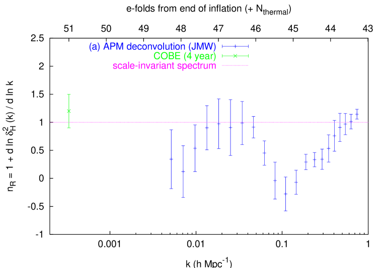
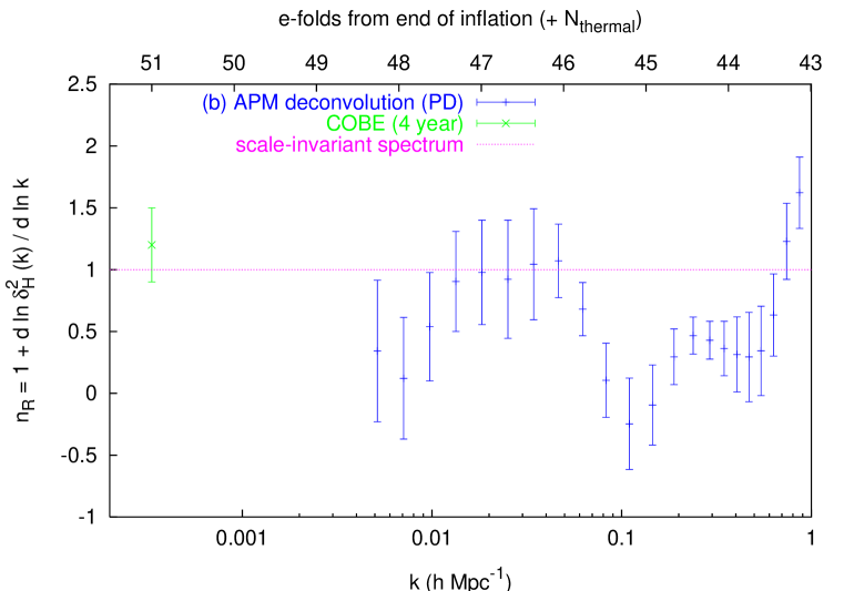
FIG. 1.: The spectral index of the primordial density perturbation implied by the APM data, assuming a critical CDM universe with $\Omega_{\rm N}=0.05$, $h=0.5$, and using two suggested procedures to extract the linear spectrum. A scale-invariant spectrum, the usually assumed generic prediction of inflation, is shown for comparison. The “notch” seen at $k\sim 0.1h$ Mpc^-1 is in accordance with the spectral feature expected due to an intermediate scale symmetry breaking phase transition.

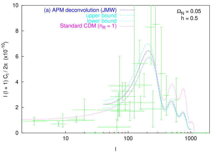
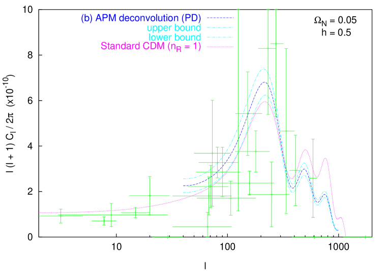
FIG. 2.: The power spectrum of CMB anisotropy implied by the APM data, assuming a critical CDM universe with $\Omega_{\rm N}=0.05$, $h=0.5$, and using two suggested procedures to extract the linear spectrum. The upper and lower envelopes correspond to the quoted $\pm 1\sigma$ errors in the APM data averaged over 4 zones. The expectation for a COBE-normalized standard CDM model (with $n_{\cal R}=1$) is shown for comparison, along with an unbiased compendium of observational data.

REFERENCES

- [1] A.D. Linde, Particle Physics and Inflationary Cosmology (Harwood Academic Press, 1990).
- [2] J. Wess and J. Bagger, Supersymmetry and Supergravity (Princeton University Press, 1993).
- [3] K.A. Olive, Phys. Rep. 190 (1990) 307.
- [4] For a review, see, D.H. Lyth, Preprint LANCS-TH/9614 (hep-ph/9609431).
- [5] G.P. Efstathiou, Physics of the Early Universe, ed. J. Peacock et al (Adam Hilger, 1990) p 361.
- [6] D. Scott and G.F. Smoot, Phys. Rev. D54 (1996) 118.
- [7] A.R. Liddle and D.H. Lyth, Phys. Rep. 231 (1993) 1.
- [8] K. Yamamoto, Phys. Lett. 161B (1985) 289, 168B (1986) 341.
-
[9]
G. Lazarides, C. Panagiotakopoulos and Q. Shafi,
Phys. Rev. Lett. 56 (1986) 557, Nucl. Phys. B307 (1988) 937;
K. Enqvist, D.V. Nanopoulos and M. Quiros, Phys. Lett. 169B (1986) 343;
O. Bertolami and G.G. Ross, Phys. Lett. 183B (1987) 163;
J. Ellis et al, Phys. Lett. B188 (1987) 415, B225 (1989) 313. - [10] V.A. Rubakov and M.E. Shaposhnikov, Usp. Fis. Nauk 166 (1996) 493.
-
[11]
I. Affleck and M. Dine, Nucl. Phys. B249 (1985) 361;
M. Dine, L. Randall and S. Thomas, Nucl. Phys. B458 (1996) 291. - [12] D.H. Lyth and E.D. Stewart, Phys. Rev. Lett. 75 (1995) 201, Phys. Rev. D53 (1996) 1784.
- [13] L. Randall and S. Thomas, Nucl. Phys. B449 (1995) 229.
- [14] G.G. Ross, Proc. 28th Intern. Conf. on High Energy Physics, 25–31 July 1996, Warsaw, eds. A.K. Wróblewski et al (World Scientific, in press).
- [15] S. Soni and A. Weldon, Phys. Lett. 126B (1983) 1215.
- [16] G. Giudice and A. Masiero, Phys. Lett. B206 (1988) 480.
- [17] R. Holman, P. Ramond and G.G. Ross, Phys. Lett. 137B (1984) 343.
- [18] G.G. Ross and S. Sarkar, Nucl. Phys. B461 (1996) 597.
-
[19]
M. Dine, W. Fischler and D. Nemechansky, Phys. Lett. 136B (1984) 169;
G.D. Coughlan et al, Phys. Lett. 140B (1984) 44. - [20] J.A. Adams, G.G. Ross and S. Sarkar, Phys. Lett. B391 (1997) 271.
- [21] M. Green, J. Schwarz and E. Witten, Superstring Theory (Cambridge University Press, 1987).
- [22] T. Barreiro et al, Phys. Rev. D54 (1996) 1379.
- [23] For a review, see, D. Boyanovsky et al, Eprint hep-ph/9701304.
-
[24]
T.T. Nakamura and E.D. Stewart, Phys. Lett. B381 (1996) 413;
M. Sasaki and E.D. Stewart, Prog. Theor. Phys. 95 (1996) 71. - [25] D.H. Lyth and E.D. Stewart, Phys. Lett. B302 (1993) 171.
-
[26]
see e.g., L.A. Kofman and D.Yu Pogosyan, Phys. Lett. 214B (1988) 508;
D.S. Salopek, J.R. Bond and J.M. Bardeen, Phys. Rev. D40 (1989) 1753;
D. Polarski and A.A. Starobinsky, Nucl. Phys. B385 (1992) 623. - [27] S. Thomas, Phys. Lett. B351 (1995) 424.
- [28] L. Kofman, A. Linde and A. Starobinsky, Phys. Rev. Lett. 76 (1996) 1011.
- [29] J. Ellis et al, Astropart. Phys. 4 (1996) 371.
- [30] S. Sarkar, Rep. Prog. Phys. 59 (1996) 1493.
- [31] G.D. Coughlan et al, Phys. Lett. 131B (1983) 59.
-
[32]
B. de Carlos et al, Phys. Lett. B318 (1993) 447;
T. Banks, D.B. Kaplan and A.E. Nelson, Phys. Rev. D49 (1994) 779. -
[33]
G.P. Efstathiou et al, Mon. Not. R. Astr. Soc 235 (1988) 715;
J.M. Gelb and E. Bertschinger, Astrophys. J. 436 (1994) 467. - [34] J.A. Peacock and S.J. Dodds, Mon. Not. R. Astr. Soc. 267 (1994) 1020.
- [35] A.J.S. Hamilton et al, Astrophys. J. 374 (1991) L1.
- [36] B. Jain, H. J. Mo and S.D.M. White, Mon. Not. R. Astr. Soc. 276 (1995) L25. (JMW)
- [37] J.A. Peacock and S.J. Dodds, Mon. Not. R. Astr. Soc. 280 (1996) L19. (PD)
- [38] C.M. Baugh and E. Gaztañaga, Mon. Not. R. Astr. Soc. 280 (1996) L37.
- [39] T. Padmanabhan, Mon. Not. R. Astr. Soc., 278 (1996) L29.
- [40] C.M. Baugh and G.P. Efstathiou, Mon. Not. R. Astr. Soc. 265 (1993) 145.
- [41] C.L. Bennett et al (COBE collab.), Astrophys. J. 464 (1996) L1.
- [42] E. Bertschinger, Eprint astro-ph/9506070 (http://arcturus.mit.edu/cosmics/).
- [43] J.A. Peacock, Mon. Not. R. Astr. Soc. 284 (1997) 885.
- [44] L.A. Kofman and A.D. Linde, Nucl. Phys. B282 (1987) 555.
- [45] M. Bucher, A.S. Goldhaber and N. Turok, Phys. Rev. D52 (1995) 3314.
- [46] For a recent review, see, P. Sikivie, Eprint hep-ph/9611339.
-
[47]
T. Banks and M. Dine, Eprint hep-th/9608197;
see also, K. Choi, E.J. Chun and J.E. Kim, Eprint hep-ph/9608222. -
[48]
J. Ellis, J. Lopez and D.V. Nanopoulos, Phys. Lett. 247B (1990) 257;
S. Sarkar, Nucl. Phys. B (Proc. Suppl.) 28A (1992) 405. - [49] M. Birkel and S. Sarkar, in preparation.