Thermal photon production rate from non-equilibrium quantum field theory

Abstract

In the framework of closed time path thermal field theory we investigate the production rate of hard thermal photons from a QCD plasma away from equilibrium. Dynamical screening provides a finite rate for chemically non-equilibrated distributions of quarks and gluons just as it does in the equilibrium situation. Pinch singularities are shown to be absent in the real photon rate even away from equilibrium.

I Introduction

Ultrarelativistic heavy ion experiments at CERN and RHIC focus on energetic direct photons as promising observables of the expected QCD plasma phase. Namely the spectrum of thermal photons could be an observable effect directly related to the multiparticle dynamics of the plasma system, and as such has been the subject of major theoretical interest. As a result the hard thermal photon spectrum has been obtained consistently in thermal field theory implementing dynamical screening mechanisms in the framework of hard-thermal-loop (HTL) resummation [1, 2, 3, 4] under the assumption that the plasma be in perfect thermal equilibrium [5, 6]. This later assumption is to be contrasted with parallel investigations of the plasma expansion [7, 8, 9, 10] from which the picture of a hot gluon gas [11] has emerged by now: quarks but also gluons are expected to be essentially undersaturated during important parts of the plasma history. The effect of this undersaturation on the photon spectrum has been examined in [12, 13, 14, 15] on the basis of folding scaled distributions on conventional matrix elements. The mass singularity appearing in this process has been cut-off by hand introducing a thermal quark mass suitably generalized from the equilibrium one. No attempt has however been made to obtain the necessary screening from a consistent treatment within thermal field theory so that the validity of this cut-off prescription seems to be ’unclear’ at the moment.

In this note we therefore examine in some detail the generalization of the HTL-resummation program to the case of undersaturated distribution functions as applied to the hard photon rate. We do so on the basis of the closed time path approach for field theoretic systems out-of-equilibrium. We take into account the appearance of recently found pinch singularities [16, 17] which can be shown to provide extra contributions to physical rates in out-of-equilibrium situations [18]. We however demonstrate that these can effectively be neglected in the present case of real photon production. Our derivation is also easily applied to the particular case of equilibrium distributions with non-vanishing chemical potential [19, 20]. Here the photon rate can be explicitly shown to be free of infrared singularities as obtained in [20] only by numerical integration of the phase space.

After giving a short review of the theoretical framework used we start with a close look on the contribution from the soft part of phase space in section II A and add the contribution from the hard part in section II B. Finally the result is obtained and discussed in section III.

II Thermal photon rate

We adopt the real time formulation of quantum field theory [21, 22] in order to calculate the photon production rate. The Keldysh variant is appropriate for a description of systems away from equilibrium [23]. Both propagators and self-energies acquire a $2\times 2$ matrix structure in this formalism. The components $(12)$ and $(21)$ of the self-energy matrix are related to the emission and absorption probability of the particle species under consideration [23, 24, 25]. In the present context we treat the photons as external probes, i.e., thermally decoupled from the quark-gluon plasma. To lowest order they are produced from annihilation and Compton processes

$$q+\bar{q}\to g+\gamma,\qquad q(\bar{q})+g\to q(\bar{q})+\gamma,$$ (1)

but there are essentially no back-reactions that would absorb photons present in the medium. The rate of photon emission can thus be calculated as

$$E\frac{dR}{d^{3}q}=\frac{i}{2(2\pi)^{3}}{\Pi_{12}}_{\mu}^{\mu}(q),$$ (2)

from the trace of the (12)-element $\Pi_{12}$ of the photon-polarization tensor.

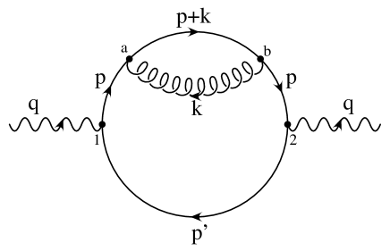
FIG. 1.: The photon polarization tensor $\Pi_{12}$ to first order in $\alpha_{s}$ for real photon production. The momentum labels define the notation used in the text. External vertices are to be of type 1 and 2, respectively, internal vertices are to be summed over $a,b=1,2$.

We calculate $\Pi_{12}$ to leading order in the strong interaction of quarks and gluons. The relevant diagram in fixed order perturbation theory is shown in Fig.1. The relevant (12) and (21) propagator components depend on the (off-equilibrium) distributions of quarks and gluons.

Having in mind locally thermalized but undersaturated distributions for quarks and gluons we neglect higher than second order terms in the cumulant expansion for the off-equilibrium correlations [23]. Separating a macroscopic scale $X$ from a fast microscopic scale $p$ in the sense of a Wigner transform and applying a gradient expansion to the former, the relevant propagators can be shown to depend on a Wigner distribution $n(X,p)$ formerly in the same way as in equilibrium [26]. For the bosonic case all relevant quantities have been listed in [18]. Sticking to the conventions used there we use the gluon propagator in Feynman gauge as

$$iD^{12}_{\mu\nu}(X,p)=-g_{\mu\nu}2\pi\varepsilon(p_{0})\delta(p^{2})n(X,p_{0}),\qquad iD_{\mu\nu}^{21}(X,p)=iD_{\nu\mu}^{12}(X,-p).$$ (3)

We choose [7, 8, 13]

$$n(X,p_{0})=n(p_{0})=\left\{\begin{array}[]{cc}\lambda_{g}n_{B}(|p_{0}|)&p_{0}>0\\ -(1+\lambda_{g}n_{B}(|p_{0}|))&p_{0}<0\end{array}\right.,$$ (4)

with $n_{B}(|p_{0}|)$ the Bose distribution in equilibrium and fugacities $\lambda_{g}$ parameterizing the deviation from chemical equilibrium for gluons. The dependence on the macroscopic variable $X$ is chosen to reside in the parameters $\lambda_{g}=\lambda_{g}(X)$ and $T=T(X)$. For our approach to be valid we assume that this macroscopic scale is large even against the soft scale $(gT)^{-1}$ for a small QCD coupling $g$ so that we differ in this respect from the assumptions discussed in [27].

Fermionic quantities are obtained by substituting fermion distributions $\tilde{n}(X,p_{0})=\tilde{n}(p_{0})$ obtained from (4) through the replacement $\lambda_{g}n_{B}\to-\lambda_{q}n_{F}$, with $n_{F}(p_{0})$ the Fermi-Dirac distribution and $\lambda_{q}$ parameterizing accordingly the deviation from equilibrium for the quark- as well as antiquark-distributions:

$$\tilde{n}(X,p_{0})=\tilde{n}(p_{0})=\left\{\begin{array}[]{cc}\lambda_{q}n_{F}(|p_{0}|)&p_{0}>0\\ 1-\lambda_{q}n_{F}(|p_{0}|))&p_{0}<0\end{array}\right..$$ (5)

We make use of the (12)-part of the fermion propagator for massless quarks which reads

$$iS_{12}(p)=-p{\kern-5.03125pt/}2\pi\delta(p^{2})\varepsilon(p_{0})\tilde{n}(X,p_{0}),\qquad iS_{21}(p)=-iS_{12}(-p).$$ (6)

All quantitative results will be given for the choice of distributions Eqs.(4) and (5). They thus fit into the framework of the model developed in [7, 8] and unnecessary technical complications are avoided because of the factorized dependence on fugacities. Our main result, i.e. the screening of the quark mass singularity, is however rather independent of this choice. It applies in particular equally well to the case of Jüttner distributions

$$n_{J}(|p_{0}|)=\frac{\lambda}{e^{|p_{0}|/T}\pm\lambda},$$ (7)

used e.g. in the analysis by Strickland [28]. Here the functional dependence on the fugacity models the introduction of a chemical potential. However this parameter takes the same value for fermions and anti-fermions, $\lambda=\lambda_{q}$, and it is also attributed to the gluons, $\lambda=\lambda_{g}$. This is to be contrasted with the equilibrium distributions, where the chemical potential $\mu$ enters with different signs for particles and antiparticles, and vanishes for gluons.

For real photons the self-energy $\Pi_{12}$ in (2) receives contributions only from spacelike loop-momenta $p^{2}\leq 0$. The fixed order result from the diagram Fig.1 turns out to contain IR singular contributions from small $p^{2}\to 0$. For the equilibrium case it has been shown that this unphysical behavior can be cured taking HTL-contributions from all orders of the quark self-energy consistently into account [5, 6]. In the spirit of the HTL-resummation program it is important to distinguish regions of hard from those of soft momenta [29]. We choose to separate these scales along the line $p^{2}=-k_{c}^{2}$ with $k_{c}^{2}$ to be chosen on an intermediate scale [5]:

$$-p^{2}_{hard}\sim T^{2}\geq k_{c}^{2}\sim gT^{2}\geq-p^{2}_{soft}\sim g^{2}T^{2}.$$ (8)

For soft momenta resummation of leading HTL-contributions from one-loop self-energy insertions is accomplished by substituting the effective resummed propagator as indicated by a blob in Fig.2. The resulting partial rate is IR finite and is shown to exactly match the hard contribution thereby introducing the thermal mass-parameter $m_{q}$ as an effective IR cut-off.

FIG. 2.: The photon polarization tensor $\Pi_{12}$ for soft momentum $p\sim gT$. The blob indicates the HTL-resummed quark propagator.

Turning to the off-equilibrium situation now our first task is to determine the appropriate generalization of the effective resummed propagator to be used on the soft scale.

A soft part

In the non-equilibrium case the analogous resummation program is complicated by the appearance of extra terms already at fixed one-loop order. Being proportional to products of basic retarded and advanced propagators

$$\Delta_{R}(p)\Delta_{A}(p)=\frac{1}{p^{2}+i\varepsilon\varepsilon(p_{0})}\frac{1}{p^{2}-i\varepsilon\varepsilon(p_{0})}=\frac{1}{(p^{2})^{2}+\varepsilon^{2}},$$ (9)

these terms are in addition plugged with pinch singularities for $p^{2}=0$ [16]. The resummed propagator for the off-equilibrium situation was discussed in [17] for the scalar case with the objective of providing a self consistent cut-off for these pinch contributions. Generalizing to the fermionic case resumming successive (one-loop) self-energy insertions

$$iS_{12}^{\star}(p)=iS_{12}^{0}+iS_{1a}^{0}(-i\Sigma_{ab})iS^{0}_{b2}+iS^{0}_{1a}(-i\Sigma_{ab})iS^{0}_{bd}(-i\Sigma_{de})iS^{0}_{e2}+\cdots$$ (10)

may be rearranged into the effective propagator

$$iS_{12}^{\star}(p) = -\tilde{n}(p_{0})(\frac{i}{p{\kern-5.03125pt/}-\Sigma+i\varepsilon p_{0}}+\frac{-i}{p{\kern-5.03125pt/}-\Sigma^{\star}-i\varepsilon p_{0}})$$ (11)

$$+ \frac{i}{p{\kern-5.03125pt/}-\Sigma+i\varepsilon p_{0}}\left[(1-\tilde{n}(p_{0}))(-i\Sigma_{12})+\tilde{n}(p_{0})(-i\Sigma_{21})\right]\frac{-i}{p{\kern-5.03125pt/}-\Sigma^{\star}-i\varepsilon p_{0}},$$ (12)

making use of the identities

$$\Sigma_{11}=-\Sigma_{22}^{\star},\qquad Im\Sigma=-\frac{i}{2}(\Sigma_{12}-\Sigma_{21}),\qquad Re\Sigma=Re\Sigma_{11},$$ (13)

where $\Sigma^{\star}$ denotes complex conjugation.

In the expression Eq.(11) $\pm i\varepsilon p_{0}$ is stated explicitly in order to keep track of the retarded or advanced nature of individual terms for later use, even though the complex thermal self-energy $\Sigma$ renders this infinitesimal displacement superfluous. With the help of Eq.(13) $\Sigma$ can be decomposed as

$$\Sigma=Re\Sigma_{11}+\frac{1}{2}(\Sigma_{12}-\Sigma_{21}).$$ (14)

Evaluating $\Sigma$ using equilibrium field theory and restricting to the leading HTL-contribution the first term in (11) reduces to the HTL-resummed effective propagator as used in the equilibrium calculations [5, 6]. The second extra term associated with pinch singularities vanishes in the equilibrium calculation because of the detailed balance relation $\Sigma_{12}=-e^{-p_{0}/T}\Sigma_{21}$. It does so as well, for the case of an equilibrium chemical potential $\mu$ applied to the quark distribution. In the general non-equilibrium situation a non-vanishing self-energy $\Sigma$ provides a self consistent cut-off for the pinch singularity in Eq.(11), as it was already observed by Altherr [17].

We proceed by evaluating the different terms of Eq.(11) in the spirit of the HTL-approximation, i.e., assuming the external momentum of the propagator to be soft and focusing only on leading self-energy contributions resulting from hard loop momenta. First, the imaginary part of $\Sigma$, Eq.(14), is linear in the distributions [26]

$$-i\Sigma^{-}(p) \equiv -\frac{i}{2}(\Sigma_{12}(p)-\Sigma_{21}(p))$$ (15)

$$= -g^{2}C_{F}\int\frac{d^{4}k}{(2\pi)^{2}}(p{\kern-5.03125pt/}+k{\kern-5.52084pt/})\delta(k^{2})\varepsilon(k_{0})\delta((p+k)^{2})\varepsilon(p_{0}+k_{0})[n(k_{0})+\tilde{n}(p_{0}+k_{0})],$$ (16)

with a color-factor $C_{F}=4/3$ for $N_{c}=3$ colors. Focusing on the leading contribution only, dimensional and angle integrations in Eq.(16) decouple,

$$\left.-i\Sigma^{-}(p)\right|_{HTL}=-\frac{g^{2}C_{F}}{2\pi}\int_{0}^{\infty}dE_{k}E_{k}(n(E_{k})+\tilde{n}(E_{k}))\int\frac{d\Omega}{4\pi}\hat{K}{\kern-5.55557pt/}~{}\delta(P\cdot\hat{K}),$$ (17)

with $\hat{K}=(1,\hat{k})$ a light-like vector with spatial direction of $\vec{k}$. In a similar way also the real part of $\Sigma$ in Eq.(14) can be analyzed in the HTL-approximation. It is found to differ from the imaginary part Eq.(17) only in the angular integrand.

The only difference to the equilibrium situation is thus seen to reside in the modified distributions to be integrated over $E_{k}=|\vec{k}|$ in Eq.(17). The combination of these functions present in Eq.(17) is important for the following discussion. Here it defines the thermal mass parameter $m_{q}$ generalized from the equilibrium case as:

$$m_{q}^{2}=\frac{g^{2}}{2\pi^{2}}C_{F}\int_{0}^{\infty}EdE(n(E)+\tilde{n}(E))=\frac{g^{2}T^{2}}{12}C_{F}\left(\lambda_{g}+\frac{\lambda_{q}}{2}\right),$$ (18)

where in the second step we perform the integration for the specific choice of distributions, Eqs.(4) and (5), respectively. There is a factor of 2 in Eq.(18) resulting from equal contributions for positive as well as negative $k_{0}$ to the integral in Eq.(16). In case of an equilibrium chemical potential $2(n(E)+\tilde{n}(E))$ is replaced by $2n_{B}(E)+n_{F}(E-\mu)+n_{F}(E+\mu)$ in the integrand of Eq.(18).

We now turn to evaluate the second, additional contribution to the propagator in Eq.(11) in HTL-approximation. The coefficient in square brackets can be decomposed as

$$(1-\tilde{n}(p_{0}))\Sigma_{12}+\tilde{n}(p_{0})\Sigma_{21}=(1-2\tilde{n}(p_{0}))\Sigma^{-}+\Sigma^{+},$$ (19)

where $\Sigma^{-}$ has already been evaluated in Eq.(17) and

$$\Sigma^{+}=\frac{1}{2}(\Sigma_{12}+\Sigma_{21})$$ (20)

is demonstrated in the following to be non-leading. It contains non-linear terms in the distribution functions:

$$-i\Sigma^{+} = g^{2}C_{F}\int\frac{d^{4}k}{(2\pi)^{2}}(p{\kern-5.03125pt/}+k{\kern-5.52084pt/})\varepsilon(k_{0})\delta(k^{2})\varepsilon(p_{0}+k_{0})\delta((p+k)^{2})$$ (22)

$$\qquad[\tilde{n}(p_{0}+k_{0})-n(k_{0})+2n(k_{0})\tilde{n}(p_{0}+k_{0})],$$

and keeping only leading contributions the angular integral decouples as before. The accompanying dimensional integral turns out to be suppressed by one power of $g$ with respect to the result (18) for soft external $p,p_{0}\sim gT$ and hard loop momentum $k\sim T$:

$$g^{2}\int_{0}^{\infty}dkk[\tilde{n}(p_{0}+k)-\tilde{n}(k-p_{0})](1+2n(k))$$ (23)

$$\quad\simeq 2p_{0}g^{2}\int_{0}^{\infty}dkk\frac{\partial}{\partial k}\tilde{n}(k)(1+2n(k))\sim O(g^{3}T^{2}).$$ (24)

This causes the contribution of $\Sigma^{+}$ in the resummed propagator Eq.(11) being of order $O(1/T)$ to be dominated by the leading contributions from $\Sigma^{-}$ and $Re\Sigma_{11}$ which are of order $O\left(1/(gT)\right)$. Neglecting therefore $\Sigma^{+}$ in Eq.(19) and substituting the remainder for the square brackets in $S^{\star}_{12}$ Eq.(11) the resummed propagator may be rearranged into a form similar to the equilibrium case [6] :

$$\left.iS_{12}^{\star}\right|_{HTL}(p)=\frac{1}{2}\varepsilon(p_{0})\left[(\gamma_{0}-\vec{\gamma}\hat{p})Im\frac{1}{\tilde{D}_{+}}+(\gamma_{0}+\vec{\gamma}\hat{p})Im\frac{1}{\tilde{D}_{-}}\right].$$ (25)

Here $\tilde{D}_{+}(p_{0},p),\tilde{D}_{-}(p_{0},p)$ determining the quark dispersion relations are as in equilibrium [30, 31, 32], however, with the thermal mass now depending on the off-equilibrium distributions as given in Eq.(18).

It is worth to point out that in equilibrium $iS^{\star}_{12}(p)$ is proportional to $n_{F}(p_{0})$, i.e. $\tilde{n}(p_{0})$ in Eq.(11) is replaced by $n_{F}(p_{0})$, which in the soft limit $p_{0}\simeq 0$ is approximated by $1/2$. This way the multiplicative factor becomes the same as in the non-equilibrium case as it is derived in Eq.(25).

In order to obtain the partial thermal photon rate from the soft part of phase space we come back to Eq.(2) and evaluate $\Pi_{12}$ from Fig.2 as

$$-i\Pi_{12}(q)=-e^{2}e_{q}^{2}N_{c}\int\frac{d^{4}p}{(2\pi)^{4}}Tr\left[\gamma^{\mu}\left.iS_{12}^{\star}(p)\right|_{HTL}\gamma_{\mu}iS_{21}(p-q)+\gamma^{\mu}iS_{12}(p)\gamma_{\mu}\left.iS_{21}^{\star}(p-q)\right|_{HTL}\right],$$ (26)

with the resummed propagator Eq.(25) and $e_{q}$ the quark charge. We now follow analogous steps as in equilibrium [5, 6]. Restricting the validity of the present resummed approach by $k_{c}\sim\sqrt{g}T$ as discussed above, the factor $1/2$ in Eq.(25) amounts to the approximation $n_{F}(p)\simeq 1/2$ applied in the equilibrium calculation. Performing the phase space integration for large $E_{\gamma}\gg T$ we find the soft contribution to the thermal photon rate

$$\left.E_{\gamma}\frac{dR}{d^{3}q}\right|_{soft}=e_{q}^{2}\frac{3\alpha}{4\pi^{3}}\lambda_{q}m_{q}^{2}e^{-E_{\gamma}/T}\ln\left[\frac{k_{c}^{2}}{2m_{q}^{2}(\lambda_{q},\lambda_{g})}\right].$$ (27)

As in the equilibrium calculation the modified thermal mass provides a self-consistent IR cut-off under the logarithm. It is crucial to note the combination of fugacities present in Eq.(27). With the appropriate changes in the thermal mass according to Eq.(18) the same result is obtained with Jüttner distributions Eq.(7). For the case of an equilibrium chemical potential $\mu<T\ll E_{\gamma}$ the multiplicative fugacity factor $\lambda_{q}$ in (27) resulting from the hard fermion line would be absent [20]. The partial rate from the hard part of phase space to which we turn next has to match this structure in order that all singularities are screened.

B hard part

For a discussion of the partial rate resulting from the region of hard exchanged/loop momentum it is convenient to introduce Mandelstam invariants from the momentum variables defined in Fig.1 as

$$s=(k+q)^{2},\quad t=p^{2}\qquad\mbox{for}\quad q+\bar{q}\to g+\gamma,$$ (28)

and accordingly for the Compton process. In terms of these the kinematic region that remains to be considered is expressed as

$$-s+k_{c}^{2}\leq p^{2}_{hard}=t\leq-k_{c}^{2},\qquad 2k_{c}^{2}\leq s\leq\infty.$$ (29)

Here the calculation is to be done in fixed order $e^{2}g^{2}$, i.e., from the diagram shown in Fig.1. We need the quark propagation with one self-energy correction. For real photon production this amounts to keeping only the second term in Eq.(10). The corresponding propagator is obtained by direct calculation of

$$i\delta S_{12}(p)=iS^{0}_{1a}(-i\Sigma_{ab})iS^{0}_{b2},$$ (30)

using the relations (14), or alternatively from an expansion of the resummed result Eq.(11). At $O(g^{2})$ the correction to the propagator is found to be

$$\delta S_{12}(p) = -\tilde{n}(p_{0})(\Delta_{R}^{2}-\Delta_{A}^{2})p{\kern-5.03125pt/}Re\Sigma(p)p{\kern-5.03125pt/}-\frac{1}{2}\tilde{n}(p_{0})(\Delta_{R}^{2}+\Delta_{A}^{2})p{\kern-5.03125pt/}(\Sigma_{12}-\Sigma_{21})p{\kern-5.03125pt/}$$ (32)

$$-\Delta_{R}\Delta_{A}p{\kern-5.03125pt/}[(1-\tilde{n}(p_{0}))\Sigma_{12}+\tilde{n}(p_{0})\Sigma_{21}]p{\kern-5.03125pt/}.$$

Here the first term, which is proportional to

$$(\Delta_{R}^{2}-\Delta_{A}^{2})=2\pi i\varepsilon(p_{0})\delta^{\prime}(p^{2}),$$ (33)

corresponds to the virtual correction to the quark propagator and does not contribute to real photon production, because the delta function has no support within the relevant region of phase space (29).

The second term would provide the result found in [5, 6], when evaluated in equilibrium. Being proportional to $Im\Sigma$ it corresponds to a vertical cut of the diagram Fig.1. Switching to Mandelstam variables $s$ and $t=p^{2}$ the factor

$$\Delta_{R}^{2}+\Delta_{A}^{2}=2{\bf P}\frac{1}{t^{2}},$$ (34)

appearing here induces a pole in the t-channel of both the Compton and annihilation process, which is to be regularized in the sense of a principal value. Together with one extra factor of t from the spin structure of the quark propagators this term is at the origin of the logarithmic mass singularity cut-off by $k_{c}^{2}$,

$$\int_{-s+k_{c}^{2}}^{-k_{c}^{2}}dt\frac{t}{t^{2}}=\ln\left(\frac{s-k_{c}^{2}}{k_{c}^{2}}\right).$$ (35)

The third term in Eq.(32) contains the pinch singular contribution Eq.(9). It can be observed though that within the region of phase space under consideration, Eq.(29), which does not include the zeros of either $s,t,u$ the common pole position is approached from $t<0$ only. In this situation both pinch and principal value turn out to be equivalent as the regularization parameter $\varepsilon$ can be taken to zero:

$$\lim_{\varepsilon\to 0}\int_{-s+k_{c}^{2}}^{-k_{c}^{2}}dt\frac{t}{t^{2}+\varepsilon^{2}}={\bf P}\int_{-s+k_{c}^{2}}^{-k_{c}^{2}}dt\frac{t}{t^{2}}=\int_{-s+k_{c}^{2}}^{-k_{c}^{2}}dt\frac{1}{t}.$$ (36)

As a result associated terms containing the distribution $\tilde{n}(p_{0})$ cancel each other. The one-loop correction to the quark propagator therefore reduces to

$$\left.\delta S_{12}(p)\right|_{p^{2}\leq-k_{c}^{2}}\stackrel{{\scriptstyle\wedge}}{{=}}-\frac{1}{(p^{2})^{2}}p{\kern-5.03125pt/}\Sigma_{12}p{\kern-5.03125pt/},$$ (37)

which agrees with the corresponding expression in thermal equilibrium up to the fact that $\Sigma_{12}$ is now to be evaluated with the more general propagators for the present situation. Calculating

$$-i\Pi_{12}(q)=-e^{2}\int\frac{d^{4}p}{(2\pi)^{4}}Tr\left[\gamma_{\mu}iS_{12}(p-q)\gamma^{\mu}i\delta S_{21}(p)+S\leftrightarrow\delta S\right],$$ (38)

we can again rely to a large extent on the work done before in the equilibrium calculation.

$\Pi_{12}$ of Eq.(38) contains contributions from both annihilation and Compton processes. The phase space integration for both partial rates may be written [33]

$$I = \int_{2k_{c}^{2}}^{\infty}ds\int_{-s+k_{c}^{2}}^{-k_{c}^{2}}\frac{dt}{s}F(s,t)\Phi(s,t,E_{\gamma};\lambda_{q},\lambda_{g}),$$ (39)

where the matrix elements $F(s,t)$ are the same as in equilibrium. In $\Phi(s,t,E_{\gamma};\lambda_{q},\lambda_{g})$ for the kinematic variables a number of integrations can be performed [33] resulting in boundaries $B_{1,2}$ for the remaining two dimensional integrations:

$$\frac{1}{s}\Phi(s,t,E_{\gamma};\lambda_{q},\lambda_{g})=\int_{B_{1}}dE_{1}n_{1}(E_{1})\int_{B_{2}}dE_{2}n_{2}(E_{2})(1\pm n_{3}(E_{1}+E_{2}-E_{\gamma}))(aE_{2}^{2}+bE_{2}+c)^{-1/2}$$ (40)

with $a,b,c$ functions of $E_{1}$. Here the actual combination of distribution functions, $n_{i}=n(n_{i}=\tilde{n})$, differs for the two processes and the sign in the enhancement (blocking) factor appears correspondingly. The expression Eq.(40) has been evaluated in previous work [5, 33] assuming Boltzmann approximation for the incoming particles with energies $E_{1},E_{2}$.

In order to obtain an IR finite emission rate it is crucial to keep full quantum statistics for the incoming particles as well in contrast to the treatment in [13, 14, 15, 19, 28]. To demonstrate this we first concentrate on the singular contribution alone which we isolate with the help of a partial integration over $d\hat{t}=-dt/s$ in Eq.(39). The contribution from the $t$-pole in the annihilation process can be written in the limit $k_{c}\to 0$:

$$I_{t-pole}^{ann} = \int_{0}^{\infty}ds\left\{\ln\left(\frac{s}{k_{c}^{2}}\right)\Phi(s,t=0,E_{\gamma};\lambda_{i})-\Phi(s,t=-s,E_{\gamma};\lambda_{i})\right\}$$ (42)

$$\qquad-\int_{0}^{\infty}ds\int_{0}^{1}d\hat{t}\left[\ln\hat{t}-\hat{t}\right]\frac{d}{d\hat{t}}\Phi(s,\hat{t},E_{\gamma};\lambda_{i}).$$

The logarithmic singularity present in the first contribution is seen to be related to processes with zero momentum transfer $t=0$ as expected. This restricts the energy of one incoming particle to coincide with the energy of the unobserved final particle:

$$\Phi_{ann}(s,t=0,E_{\gamma})=\frac{\pi^{2}}{E_{\gamma}}\tilde{n}(E_{\gamma})\int_{s/4E_{\gamma}}^{\infty}dE\tilde{n}(E)(1+n(E)).$$ (43)

The same expression is found for the phase space $\Phi_{ann}(s,u=0,E_{\gamma})$ weighting the singular contribution from the $u$-pole in the annihilation process. The Compton process on the other hand contributes two singular terms from quark as well as anti-quark scattering each weighted by

$$\Phi_{com}(s,t=0,E_{\gamma})=\Phi_{com}(s,u=0,E_{\gamma})=\frac{\pi^{2}}{E_{\gamma}}\tilde{n}(E_{\gamma})\int_{s/4E_{\gamma}}^{\infty}dEn(E)(1-\tilde{n}(E)).$$ (44)

Summing finally all four singular contributions, products of distribution functions under the remaining integral cancel between the two processes leaving behind the same linear combination $2[n(E)+\tilde{n}(E)]$ as it appeared in the definition of the thermal mass Eq.(18). This is crucial for the latter to provide the necessary cut-off. Treating quarks and anti-quarks differently for the case of an equilibrium chemical potential the fermionic distributions in Eqs.(43) and (44) have to be adjusted correspondingly summing again to $2n_{B}(E)+n_{F}(E-\mu)+n_{F}(E+\mu)$ defining the thermal mass in this case. On the other hand from Eqs.(43) and (44) it is also evident that applying the Boltzmann approximation to the incoming particles spoils this nice feature in either case, and therefore the singularity remains under this approximation.

Interchanging the remaining two integrations over $s$ and $E_{1}$ and again assuming the photon energy to be large with respect to $T$, i.e., $\tilde{n}(E_{\gamma})\simeq\lambda_{q}e^{-E_{\gamma}/T}$, the singular part of the rate in the off-equilibrium situation is now easily obtained as

$$\left.E\frac{dR^{sing}}{d^{3}q}\right|_{hard}=e_{q}^{2}\frac{3\alpha}{4\pi^{3}}\lambda_{q}m_{q}^{2}e^{-E_{\gamma}/T}\ln\left(\frac{4E_{\gamma}T}{k_{c}^{2}}\right).$$ (45)

In order to complete the calculation we treat the remaining two contributions in Eq.(42) in order to fix the constant under the logarithm in Eq.(45). This requires the unrestricted kinematic phase space $\Phi(s,t,E_{\gamma};\lambda_{q},\lambda_{g})$ to be calculated with full quantum distributions. This can be accomplished by expanding Bose and Fermi distributions as

$$n_{F}(p_{0})=\sum_{n=1}^{\infty}(-)^{n+1}e^{-n\beta p_{0}},\qquad n_{B}(p_{0})=\sum_{n=1}^{\infty}e^{-n\beta p_{0}}.$$ (46)

For the equilibrium case the resulting extra contributions have been shown to cancel between the annihilation and Compton channel [6] making the Boltzmann approximation for the final result better than it is to be expected on the basis of individual processes [5]. This cancellation, however, depends on the properties of the equilibrium Fermi-Dirac and Bose-Einstein distributions and is spoiled for the off-equilibrium situation. For the specific choice Eqs.(4) and (5) the additional contributions can nevertheless be evaluated without having to resort to classical approximations. We choose to order the resulting terms according to the powers of fugacities present, having in mind that eventually $\lambda_{q}\ll\lambda_{g}$. Taking out one common factor $\lambda_{q}$ we obtain for the remaining contribution

$$\left.E_{\gamma}\frac{dR^{const}}{d^{3}q}\right|_{hard} = e_{q}^{2}\frac{2\alpha\alpha_{s}}{\pi^{4}}e^{-E_{\gamma}/T}T^{2}\lambda_{q}~{}C(E_{\gamma},T,\lambda_{q},\lambda_{g}),$$ (47)

with

$$C(E_{\gamma},T,\lambda_{q},\lambda_{g}) = \lambda_{q}\left[-1+(1-\frac{\pi^{2}}{6})\gamma+(1-\frac{\pi^{2}}{12})\ln\frac{E_{\gamma}}{T}+\zeta_{-}\right]$$ (50)

$$\quad+\lambda_{g}\left[\frac{1}{2}+(1-\frac{\pi^{2}}{3})\gamma+(1-\frac{\pi^{2}}{6})\ln\frac{E_{\gamma}}{T}-\zeta_{+}\right]$$

$$\quad+\lambda_{q}\lambda_{g}\left[\frac{1}{2}-\frac{\pi^{2}}{8}+(\frac{\pi^{2}}{4}-2)(\gamma+\ln\frac{E_{\gamma}}{T})+\frac{3}{2}\zeta^{\prime}(2)+\frac{\pi^{2}}{12}\ln 2+(\zeta_{+}-\zeta_{-})\right].$$

The appearing symbols are Euler’s constant $\gamma$, the derivative of the Riemann $\zeta$-function evaluated at $\zeta^{\prime}(2)$ and the sums

$$\zeta_{+}=\sum_{n=2}^{\infty}\frac{1}{n^{2}}\ln(n-1)\simeq 0.67,\qquad\zeta_{-}=\sum_{n=2}^{\infty}\frac{(-)^{n}}{n^{2}}\ln(n-1)\simeq-0.04.$$ (51)

The result Eq.(50) is successfully checked for consistency by noting that the constants present in the equilibrium result [6] are reproduced for $\lambda_{q}=\lambda_{g}=1$.

Summarizing this subsection we find the partial rate for photon emission from the hard part of phase space, Eq.(29), to be given by the sum of the two contributions Eq.(45) and (50),

$$\left.E\frac{dR}{d^{3}q}\right|_{hard}=\left.E\frac{dR^{sing}}{d^{3}q}\right|_{hard}+\left.E\frac{dR^{const}}{d^{3}q}\right|_{hard}.$$ (52)

III result and conclusions

Calculating the complete emission rate for real photons as the sum of the two partial rates Eqs.(27) and (52) we see that the dependence on the arbitrarily chosen $k_{c}$ cancels. In the process the generalized thermal mass is established as self consistent cut-off for the logarithmic singularity thereby justifying the approach taken in previous work. Our result can be written

$$E_{\gamma}\frac{dR}{d^{3}q}=e_{q}^{2}\frac{\alpha\alpha_{s}}{2\pi^{2}}\lambda_{q}T^{2}e^{-E_{\gamma}/T}\left[\frac{2}{3}(\lambda_{g}+\frac{\lambda_{q}}{2})\ln\left(\frac{2E_{\gamma}T}{m_{q}^{2}}\right)+\frac{4}{\pi^{2}}C(E_{\gamma},T,\lambda_{q},\lambda_{g})\right].$$ (53)

The dynamical screening of the mass singularity actually does not depend on the explicit form, Eqs.(4) and (5), of the distribution functions assumed in Eq.(53). In fact it only relies on the crucial combination of distributions used to define the thermal mass in Eq.(18) to appear in front of the singular factor from the sum of Eq.(43) and (44). In particular Jüttner distributions Eq.(7) lead to a result differing in the thermal mass parameter and the constant factors under the logarithm, but the photon spectrum is equally free of singularities. The same conclusion holds also for an equilibrium situation with a non-vanishing chemical potential [20].

The second important result of our analysis is that we show explicitly the absence of any additional contributions from pinch singular terms to the off-equilibrium photon production rate (53). As far as the soft momentum scale contribution is concerned these terms are shown to be subleading with respect to the dominant HTL-contributions. For the hard scale on the other hand the absence of pinch singular contributions is due to the restricted kinematics of real photon production and does not apply in general, e.g., for virtual photon production the relevant region of phase space is sufficiently enlarged for these terms to become relevant [18, 26].

Turning finally to more quantitative conclusions we note that the rate Eq.(53) differs in details from the results of both Refs.[12] and [13]; but indeed justifies the cut-off prescription employed therein. The discrepancy with respect to [13] can be attributed to the fact that distributions for the incoming particles have been treated in Boltzmann approximation. We find however that it is necessary to keep track of full quantum statistics in order for the screening to be complete. Following [12] we finally obtain a handy estimate by restricting to the idealized situation of a fully saturated gluon distribution $\lambda_{g}=1$ with a quark admixture below its equilibrium value by a factor $\lambda_{q}=\zeta=1/4$ . In this situation the photon rate is approximated by

$$E_{\gamma}\frac{dR}{d^{3}q}\simeq e_{q}^{2}\frac{\alpha\alpha_{s}}{3\pi^{2}}T^{2}e^{-E_{\gamma}/T}(\zeta+\frac{\zeta^{2}}{2})\ln\left(\frac{cE_{\gamma}}{g^{2}T}\right).$$ (54)

There is an overall factor 2 with respect to [12] and a rather large constant $c\simeq 5$ under the logarithm depending on the actual value of $E_{\gamma}/T$.

According to (54) the photon emission rate is reduced by a factor of about $3/8$ with respect to the equilibrium case; this reduction is however easily compensated by a higher plasma temperature.

Acknowledgments

One of us K. R. acknowledges partial support of the Gesellschaft für Schwerionenforschung (GSI) and of the Committee of Research Development (KBN 2-P03B-09908). This work is supported in part by the EEC Programme ”Human Capital and Mobility”, Network ”Physics at High Energy Colliders”, Contract CHRX-CT93-0357. M. D. is supported by Deutsche Forschungsgemeinschaft.

REFERENCES

- [1] R. Pisarski, Phys. Rev. Lett. 63, 1129 (1989).
- [2] E. Braaten and R. Pisarski, Nucl. Phys. B337, 569 (1990).
- [3] R. Pisarski, Nucl. Phys. A525, 175c (1991).
- [4] J. Frenkel and J. Taylor, Nucl. Phys. B339, 199 (1990).
- [5] J. Kapusta, P. Lichard, and D. Seibert, Phys. Rev. D44, 2774 (1991).
- [6] R. Baier, H. Nakkagawa, A. Niegawa, and K. Redlich, Z. Phys. C53, 433 (1992).
- [7] T. S. Biro et al., Phys. Rev. C48, 1275 (1993).
- [8] T. S. Biro, M. H. Thoma, B. Müller, and X. N. Wang, Nucl. Phys. A566, 543c (1994).
- [9] S. M. H. Wong, Phys. Rev. C54, 2588 (1996).
- [10] K. Geiger and J. Kapusta, Phys. Rev. D47, 4905 (1993).
- [11] E. Shuryak, Phys. Rev. Lett. 68, 3270 (1992).
- [12] E. Shuryak and L. Xiong, Phys. Rev. Lett. 70, 2241 (1993).
- [13] M. H. Thoma and C. T. Traxler, Phys. Rev. C53, 1348 (1996).
- [14] B. Kämpfer and O. Pavlenko, Z. Phys. C 62, 491 (1994).
- [15] D. K. Srivastava, M. G. Mustafa, and B. Müller, nucl-th/9611041 (unpublished) (1996).
- [16] T. Altherr and D. Seibert, Phys. Lett. B 333, 149 (1994).
- [17] T. Altherr, Phys. Lett. B 341, 325 (1995).
- [18] R. Baier, M. Dirks, and K. Redlich, Phys. Rev. D55, 4344 (1997).
- [19] A. Dumitru, D. Rischke, H. Stöcker, and W. Greiner, Mod. Phys. Lett. A8, 1291 (1993).
- [20] C. T. Traxler, H. Vija, and M. H. Thoma, Phys. Lett. B346, 329 (1995).
- [21] N. P. Landsman and C. G. van Weert, Phys. Rep. 145, 141 (1987).
- [22] M. Le Bellac, Thermal Field Theory (Cambridge University Press, Cambridge, 1996).
- [23] K.-C. Chou, Z.-B. Su, B.-L. Hao, and L. Yu, Phys. Rep. 118, 1 (1985).
- [24] S. Mrowczynski and U. Heinz, Ann. Phy. 229, 1 (1994).
- [25] E. Calzetta and B. Hu, Phys. Rev. D 37, 2878 (1988).
- [26] M. Le Bellac and H. Mabilat, pp INLN 96/17 (unpublished) (1996).
- [27] J.-P. Blaizot, J. Ollitrault, and E. Iancu, in Quark-Gluon Plasma II, edited by R. Hwa (World Scientific, Singapore, 1995).
- [28] M. Strickland, Phys. Lett. B331, 245 (1994).
- [29] E. Braaten and T. C. Yuan, Phys. Rev. Lett. 66, 2183 (1991).
- [30] H. Weldon, Phys. Rev. D26, 2789 (1982).
- [31] H. Weldon, Phys. Rev. D40, 2410 (1989).
- [32] R. D. Pisarski, Nucl. Phys. A498, 423c (1989).
- [33] G. Staadt, W. Greiner, and J. Rafelski, Phys. Rev. D33, 66 (1985).