Soft gluon effects on lepton pairs at hadron colliders

Abstract

With a large integrated luminosity expected at the Tevatron, a next-to-leading order (NLO) calculation is no longer sufficient to describe the data which yield the precision measurement of $M_{W}$, etc. Thus, we extend the Collins-Soper-Sterman resummation formalism, for on-shell vector boson production, to correctly include the effects of the polarization and the width of the vector boson to the distributions of the decay leptons. We show how to test the rich dynamics of the QCD multiple soft gluon radiation, for example, by measuring the ratio $R_{CSS}\equiv\frac{\sigma(Q_{T}>Q_{T}^{\min})}{\sigma_{Total}}$. ($Q_{T}$ is the transverse momentum of the vector boson.) We conclude that both the total rates and the distributions of the lepton charge asymmetry predicted by the resummed and the NLO calculations are different when kinematic cuts are applied.

I Introduction

Quantum Chromodynamics (QCD) is a field theory that is expected to explain all the experimental data involving strong interactions either perturbatively or non-perturbatively [1]. Consider the weak boson ($W^{\pm}$ and $Z^{0}$) production at a hadron collider, such as the Tevatron. In the framework of QCD the production rate of the weak bosons is calculated by multiplying the constituent cross section (the short-distance or the perturbative physics) by the parton luminosities (the long-distance or the non-perturbative physics) [2]. This prescription of theoretical calculation was proven to the accuracy of ${\cal O}(1/Q^{2})$ and is known as the factorization theorem of QCD [3]. ($Q$ is the mass of the vector boson.) Since we do not yet know how to solve QCD exactly, we have to rely on the factorization theorem to separate the perturbative part from the non-perturbative part of the formalism for any physical observable. The short distance contribution can be calculated perturbatively order by order in the strong coupling $\alpha_{S}$. The long distance part has to be parametrized and fitted to the existing data so that it can later be used to predict the results of new experiments. Therefore, theoretical predictions that are compared to experimental data always has to invoke some approximation in the calculations based upon QCD. We refer to different prescriptions of calculations to be different models of theory calculations which all originate from the one and only QCD theory. For instance, to improve theory predictions on the event shape, such as the transverse momentum ($Q_{T}$) distribution of the weak boson, the commonly used theory model is the event generator, e.g., ISAJET [4], PYTHIA [5], or HERWIG [6]. The event generator can also provide information on the particle multiplicities or the number of jets, etc.

However, as discussed above, different models of calculation make different approximations. Hence, a model can give more reliable theory predictions than the others on some observables, but may do worse for the other observables. A few more examples are in order. To calculate the total production rate of a weak boson at hadron colliders, it is better to use a fixed order perturbation calculation, and a higher order calculation is usually found to be more reliable than a lower order calculation because it is usually less sensitive to the choice of the scale for calculating the parton distribution functions (PDF) or the constituent cross section (including the strong coupling constant $\alpha_{S}$). The former scale is the factorization scale and the latter is the renormalization scale of the process. Unfortunately, a fixed order perturbation calculation cannot give reliable prediction of the distribution of $Q_{T}$ when $Q_{T}$ is small. On the contrary, an event generator can give more reliable prediction for $Q_{T}$ distribution in the small $Q_{T}$ region, but it usually does not predict an accurate event rate. The general feature of the above two theory models is that a fixed order calculation is more reliable for calculating the event rate but not the event shape, and an event generator is good for predicting the event shape but less reliable for the event rate.

In this paper, we discuss another model of theory calculation that can give reliable predictions on both the event rate and the shape of the distributions. Specifically, we are interested in the distributions of the weak bosons and their decay products. This model of calculation is to resum a series of large perturbative contributions due to soft gluon emission predicted by the QCD theory. We present the QCD resummation formalism for calculating the fully differential cross section of the hadronically produced lepton pairs through electroweak (EW) vector boson production and decay: $h_{1}h_{2}\rightarrow V(\rightarrow\ell_{1}{\bar{\ell}_{2}})X$. We focus our attention on the Tevatron though our calculation is general and applicable for any hadronic initial state $h_{1}h_{2}$ and any colorless vector boson. For instance, the vector boson $V$ can be one of the standard model (SM) electroweak gauge bosons $W^{\pm}$ or $Z^{0}$, the virtual photon $\gamma^{*}$ (for producing the Drell-Yan pair), or some exotic vector boson such as $Z^{\prime}$ and $W^{\prime}$ in the extended unified gauge theories.

At the Tevatron, about ninety percent of the production cross section of the $W^{\pm}$ and $Z^{0}$ bosons (with mass $Q$) is in the small transverse momentum ($Q_{T}$) region, where $Q_{T}\lesssim 20$ GeV (hence $Q_{T}^{2}\ll Q^{2}$). In this region the higher order perturbative corrections, dominated by soft and collinear gluon radiation, of the form $Q_{T}^{-2}\sum_{n=1}^{\infty}\sum_{m=0}^{2n-1}{}_{n}v_{m}\,\alpha_{S}^{n}\ln^{m}({Q_{T}^{2}/Q^{2}})$, are substantial because of the logarithmic enhancement [7]. (${}_{n}v_{m}$ are the coefficient functions for a given $n$ and $m$.) These corrections are divergent in the $Q_{T}\rightarrow 0$ limit at any fixed order of the perturbation theory. After applying the renormalization group analysis, these singular contributions in the low $Q_{T}$ region can be resummed to derive a finite prediction for the $Q_{T}$ distribution to compare with experimental data. It was proven by Collins and Soper in Ref. [8] that not only the leading logs [9, 10] but all the large logs, including the sub-logs in the perturbative, order-by-order calculations can be resummed for the energy correlation in $e^{+}e^{-}$ collisions.

For the production of vector bosons in hadron collisions two different formalisms were presented in the literature to resum the large contributions due to multiple soft gluon radiation: by Altarelli, Ellis, Greco, Martinelli (AEGM) [11]; and by Collins, Soper and Sterman (CSS) [7]. The detailed differences between these two formalisms were discussed in Ref. [12]. It was shown that the AEGM and the CSS formalisms are equivalent up to the few highest power of $\ln({Q_{T}^{2}/Q^{2}})$ at every order in $\alpha_{S}$ for terms proportional to ${Q}_{T}^{-2}$, provided $\alpha_{S}\,$ in the AEGM formalism is evaluated at $b_{0}^{2}/b^{2}$ rather than at ${Q^{2}}$. A more noticeable difference, except the additional contributions of order ${Q}^{-2}$ included in the AEGM formula, is caused by different ways of parametrizing the non-perturbative contribution in the low $Q_{T}$ regime. Since the CSS formalism was proven to sum over not just the leading logs but also all the sub-logs, and the piece including the Sudakov factor was shown to be renormalization group invariant [7], we only discuss the results of CSS formalism in the rest of this paper.

With the increasing accuracy of the experimental data on the properties of $W^{\pm}$ and $Z^{0}$ bosons at the Tevatron, it is no longer sufficient to only consider the effects of multiple soft gluon radiation for an on-shell vector boson and ignore the effects coming from the decay width and the polarization of the massive vector boson to the distributions of the decay leptons. Hence, it is desirable to have an equivalent resummation formalism [13] for calculating the distributions of the decay leptons. This formalism should correctly include the off-shellness of the vector boson (i.e. the effect of the width ) and the polarization information of the produced vector boson which determines the angular distributions of the decay leptons.

In the next section, we give our analytical results for such a formalism that correctly takes into account the effects of the multiple soft gluon radiation on the distributions of the decay leptons from the vector boson. In Section III, we discuss the phenomenology predicted by this resummation formalism. To illustrate the effects of multiple soft gluon radiation, we also give results predicted from a next-to-leading order (NLO) calculation. As expected, the observables that are directly related to the transverse momentum of the vector boson will show large differences between the resummed and the NLO predictions. These observables are the transverse momentum of the leptons from vector boson decay, the back-to-back correlations of the leptons from $Z^{0}$ decay, etc. The observables that are not directly related to the transverse momentum of the vector boson can also show noticeable differences between the resummed and the NLO calculations if the kinematic cuts applied to select the signal events are strongly correlated to the transverse momentum of the vector boson. Section IV contains our detailed discussion.

Since this $Q_{T}$ resummation formalism only holds in the Collins-Soper ($CS$) frame [14], we give the detailed form of the transformation between a four-momentum in the $CS$ frame (a special rest frame of the vector boson) and that in the laboratory frame (the center-of-mass frame of the hadrons $h_{1}$ and $h_{2}$) in Appendix A. In Appendix B the analytical expression for the NLO results, of ${\cal{O}}(\alpha_{S})$, are given in $D=4-2\epsilon$ dimensions. Appendix C contains the expansion of the resummation formula up to ${\cal O}(\alpha_{S})$. Appendix D lists the values of $A$, $B$, and $C$ functions (cf. Sec. II) used for our numerical calculations.

We note that the resummation formalism presented in this paper can be applied to any processes of the type $h_{1}h_{2}\rightarrow V(\rightarrow\ell_{1}{\bar{\ell}_{2}})X$, where $V$ is a color neutral vector boson which couples to quarks and leptons via vector or axial vector currents, that is $V=e\gamma,W^{\pm},Z^{0},W^{\prime},Z^{\prime}$, etc. Throughout this paper, we take $V$ to be either $W^{\pm}$ or $Z^{0}$ bosons, unless specified otherwise.

II The Resummation Formalism

To derive the resummation formalism, we use the dimensional regularization scheme to regulate the infrared divergencies, and adopt the canonical-$\gamma_{5}$ prescription to calculate the anti-symmetric part of the matrix element in $D$-dimensional space-time. The infrared-anomalous contribution arising from using the canonical-$\gamma_{5}$ prescription was carefully handled by applying the procedures outlined in Ref. [18] for calculating both the virtual and the real diagrams.

The kinematics of the vector boson $V$ (real or virtual) can be expressed in terms of its mass $Q$, rapidity $y$, transverse momentum $Q_{T}$, and azimuthal angle $\phi_{V}$, measured in the laboratory frame (the center-of-mass frame of hadrons $h_{1}$ and $h_{2}$). The kinematics of the lepton $\ell_{1}$ is described by $\theta$ and $\phi$, the polar and the azimuthal angles, defined in the Collins-Soper frame [14], which is a special rest frame of the $V$-boson [19]. (A more detailed discussion of the kinematics can be found in Appendix A.) The fully differential cross section for the production and decay of the vector boson is given by the resummation formula in Ref. [13]:

$$\left({\frac{d\sigma(h_{1}h_{2}\rightarrow V(\rightarrow\ell_{1}{\bar{\ell}_{2}})X)}{dQ^{2}\,dy\,dQ_{T}^{2}\,d\phi_{V}\,d\cos{\theta}\,d\phi}}\right)_{res}={\frac{1}{96\pi^{2}S}}\,{\frac{Q^{2}}{(Q^{2}-M_{V}^{2})^{2}+Q^{4}\Gamma_{V}^{2}/M_{V}^{2}}}$$ (1)

$$~{}~{}\times\left\{{\frac{1}{(2\pi)^{2}}}\int d^{2}b\,e^{i{\vec{Q}_{T}}\cdot{\vec{b}}}\,\sum_{j,k}{\widetilde{W}_{j{\bar{k}}}(b_{*},Q,x_{1},x_{2},\theta,\phi,C_{1},C_{2},C_{3})}\,\widetilde{W}_{j{\bar{k}}}^{NP}(b,Q,x_{1},x_{2})\right.$$ (2)

$$~{}~{}~{}~{}\left.+~{}Y(Q_{T},Q,x_{1},x_{2},\theta,\phi,{C_{4}})\right\}.$$ (3)

In the above equation the parton momentum fractions are defined as $x_{1}=e^{y}Q/\sqrt{S}$ and $x_{2}=e^{-y}Q/\sqrt{S}$, where $\sqrt{S}$ is the center-of-mass (CM) energy of the hadrons $h_{1}$ and $h_{2}$. For $V=W^{\pm}$ or $Z^{0}$, we adopt the LEP line-shape prescription of the resonance behavior. The renormalization group invariant quantity $\widetilde{W}_{j{\bar{k}}}(b)$, which sums to all orders in $\alpha_{S}$ all the singular terms that behave as $Q_{T}^{-2}$ $\times$ [1 or $\ln{(Q_{T}^{2}/Q^{2})}$] for $Q_{T}\rightarrow 0$, is

$$\widetilde{W}_{j{\bar{k}}}(b,Q,x_{1},x_{2},\theta,\phi{,C_{1},C_{2},C_{3}})=\exp\left\{-{\cal S}(b,Q{,C_{1},C_{2}})\right\}\mid V_{jk}\mid^{2}$$ (4)

$$~{}\times\left\{\left[\left(C_{ja}\otimes f_{a/h_{1}}\right)(x_{1})~{}\left(C_{{\bar{k}}b}\otimes f_{b/h_{2}}\right)(x_{2})+\left(C_{{\bar{k}}a}\otimes f_{a/h_{1}}\right)(x_{1})~{}\left(C_{jb}\otimes f_{b/h_{2}}\right)(x_{2})\right]\right.$$ (5)

$$~{}~{}~{}~{}~{}\times(g_{L}^{2}+g_{R}^{2})(f_{L}^{2}+f_{R}^{2})(1+\cos^{2}\theta)$$ (6)

$$~{}~{}~{}+\left[\left(C_{ja}\otimes f_{a/h_{1}}\right)(x_{1})~{}\left(C_{{\bar{k}}b}\otimes f_{b/h_{2}}\right)(x_{2})-\left(C_{{\bar{k}}a}\otimes f_{a/h_{1}}\right)(x_{1})~{}\left(C_{jb}\otimes f_{b/h_{2}}\right)(x_{2})\right]$$ (7)

$$~{}~{}~{}~{}~{}\left.\times(g_{L}^{2}-g_{R}^{2})(f_{L}^{2}-f_{R}^{2})(2\cos\theta)\right\},$$ (8)

where $\otimes$ denotes the convolution

$$\left(C_{ja}\otimes f_{a/h_{1}}\right)(x_{1})=\int_{x_{1}}^{1}{\frac{d\xi_{1}}{\xi_{1}}}\,C_{ja}\left({\frac{x_{1}}{\xi_{1}}},b,\mu=\frac{C_{3}}{b},C_{1},C_{2}\right)\;f_{a/h_{1}}\left(\xi_{1},\mu=\frac{C_{3}}{b}\right),$$ (9)

and the $V_{jk}$ coefficients are given by

$$V_{jk}=\cases{{\rm Cabibbo-Kobayashi-Maskawa~{}matrix~{}elements}&for $V=W^{\pm}$\cr$$\delta_{jk}$$&for $V=Z^{0},\gamma^{*}$}.$$ (10)

In the above expressions $j$ represents quark flavors and $\bar{k}$ stands for anti-quark flavors. The indices $a$ and $b$ are meant to sum over quarks and anti-quarks or gluons. Summation on these double indices is implied. In Eq. (8) we define the couplings $f_{L,R}$ and $g_{L,R}$ through the $\ell_{1}{\bar{\ell}_{2}}V$ and the $q{\bar{q}^{\prime}}V$ vertices, which are written respectively, as

$$i\gamma_{\mu}\left[f_{L}(1-\gamma_{5})+f_{R}(1+\gamma_{5})\right]~{}~{}~{}{\rm and}~{}~{}~{}i\gamma_{\mu}\left[g_{L}(1-\gamma_{5})+g_{R}(1+\gamma_{5})\right].$$

For example, for $V=W^{+},q=u$, ${\bar{q}^{\prime}}={\bar{d}}$, $\ell_{1}=\nu_{e}$, and ${\bar{\ell}_{2}}=e^{+}$, the couplings $g_{L}^{2}=f_{L}^{2}=G_{F}M_{W}^{2}/\sqrt{2}$ and $g_{R}^{2}=f_{R}^{2}=0$, where $G_{F}$ is the Fermi constant. The detailed information on the values of the parameters used in Eqs. (3) and (8) is given in Table I. The Sudakov exponent ${\cal S}(b,Q{,C_{1},C_{2}})$ in Eq. (8) is defined as

$${\cal S}(b,Q{,C_{1},C_{2}})=\int_{C_{1}^{2}/b^{2}}^{C_{2}^{2}Q^{2}}{\frac{d{\bar{\mu}}^{2}}{{\bar{\mu}}^{2}}}\left[A\left(\alpha_{S}({\bar{\mu}}),C_{1}\right)\ln\left({\frac{C_{2}^{2}Q^{2}}{{\bar{\mu}}^{2}}}\right)+B\left(\alpha_{S}({\bar{\mu}}),C_{1},C_{2}\right)\right].$$ (11)

The explicit forms of the $A$, $B$ and $C$ functions and the renormalization constants $C_{i}$ ($i$=1,2,3) are summarized in Appendix D.

$V$	$M_{V}$ (GeV)	$\Gamma_{V}$ (GeV)	$g_{L}$	$g_{R}$
$\gamma$	0.00	0.00	$gQ_{f}s_{w}/2$	$gQ_{f}s_{w}/2$
$W^{\pm}$	80.36	2.07	$g/(2\sqrt{2})$	0
$Z^{0}$	91.19	2.49	$g(T_{3}-Q_{f}s_{w}^{2})/(2c_{w})$	$-gQ_{f}s_{w}^{2}/(2c_{w})$

TABLE I.: Vector boson parameters and couplings to fermions. The $f{\bar{f}^{\prime}}V$ vertex is defined as $i\gamma_{\mu}[g_{L}(1-\gamma_{5})+g_{R}(1+\gamma_{5})]$ and $s_{w}=\sin\theta_{w}$ ($c_{w}=\cos\theta_{w}$) is the sine (cosine) of the weak mixing angle: $\sin^{2}(\theta_{w}(M_{Z^{0}}))_{\overline{MS}}=0.2315$. $Q_{f}$ is the fermion charge ($Q_{u}=2/3,Q_{d}=-1/3,Q_{e^{-}}=-1,Q_{\nu}=0$), and $T_{3}$ is the eigenvalue of the third component of the $SU(2)_{L}$ generator ($T_{3}^{u}=1/2$, $T_{3}^{d}=-1/2$, $T_{3}^{\nu}=1/2$, $T_{3}^{e^{-}}=-1/2$).

In Eq. (3) the magnitude of the impact parameter $b$ is integrated from 0 to $\infty$. However, in the region where $b\gg 1/\Lambda_{QCD}$, the Sudakov exponent ${\cal S}(b,Q,C_{1},C_{2})$ diverges as the result of the Landau pole of the QCD coupling $\alpha_{S}(\mu)$ at $\mu=\Lambda_{QCD}$, and the perturbative calculation is no longer reliable. As discussed in the previous section, in this region of the impact parameter space (i.e. large $b$), a prescription for parametrizing the non-perturbative physics in the low $Q_{T}$ region is necessary. Following the idea of Collins and Soper [8], the renormalization group invariant quantity $\widetilde{W}_{j{\bar{k}}}(b)$ is written as

$$\widetilde{W}_{j{\bar{k}}}(b)=\widetilde{W}_{j{\bar{k}}}(b_{*})\widetilde{W}_{j{\bar{k}}}^{NP}(b)\,.$$

Here $\widetilde{W}_{j{\bar{k}}}(b_{*})$ is the perturbative part of $\widetilde{W}_{j{\bar{k}}}(b)$ and can be reliably calculated by perturbative expansions, while $\widetilde{W}_{j{\bar{k}}}^{NP}(b)$ is the non-perturbative part of $\widetilde{W}_{j{\bar{k}}}(b)$ that cannot be calculated by perturbative methods and has to be determined from experimental data. To test this assumption, one should verify that there exists a universal functional form for this non-perturbative function $\widetilde{W}_{j{\bar{k}}}^{NP}(b)$. This is similar to the general expectation that there exists a universal set of parton distribution functions (PDF’s) that can be used in any perturbative QCD calculation to compare it with experimental data. In the perturbative part of $\widetilde{W}_{j{\bar{k}}}(b)$,

$$b_{*}={\frac{b}{\sqrt{1+(b/b_{max})^{2}}}}\,,$$

and the non-perturbative function was parametrized by (cf. Ref. [7])

$$\widetilde{W}_{j\bar{k}}^{NP}(b,Q,Q_{0},x_{1},x_{2})=\exp\left[-F_{1}(b)\ln\left(\frac{Q^{2}}{Q_{0}^{2}}\right)-F_{j/{h_{1}}}(x_{1},b)-F_{{\bar{k}}/{h_{2}}}(x_{2},b)\right],$$ (12)

where $F_{1}$, $F_{j/{h_{1}}}$ and $F_{{\bar{k}}/{h_{2}}}$ have to be first determined using some sets of data, and later can be used to predict the other sets of data to test the dynamics of multiple gluon radiation predicted by this model of the QCD theory calculation. As noted in Ref. [7], $F_{1}$ does not depend on the momentum fraction variables $x_{1}$ or $x_{2}$, while $F_{j/{h_{1}}}$ and $F_{{\bar{k}}/{h_{2}}}$ in general depend on those kinematic variables. The $\ln(Q^{2}/Q_{0}^{2})$ dependence associated with the $F_{1}$ function was predicted by the renormalization group analysis [7]. Furthermore, $F_{1}$ was shown to be universal, and its leading behavior ($\sim b^{2}$) can be described by renormalon physics [20]. Various sets of fits to these non-perturbative functions can be found in Refs. [21] and [22].

In our numerical results in the next section, we use the Ladinsky-Yuan parametrization of the non-perturbative function (cf. Ref. [22]):

$$\widetilde{W}_{j\bar{k}}^{NP}(b,Q,Q_{0},x_{1},x_{2})={\rm exp}\left[-g_{1}b^{2}-g_{2}b^{2}\ln\left({Q\over 2Q_{0}}\right)-g_{1}g_{3}b\ln{(100x_{1}x_{2})}\right],$$ (13)

where $g_{1}=0.11^{+0.04}_{-0.03}~{}{\rm GeV}^{2}$, $g_{2}=0.58^{+0.1}_{-0.2}~{}{\rm GeV}^{2}$, $g_{3}=-1.5^{+0.1}_{-0.1}~{}{\rm GeV}^{-1}$ and $Q_{0}=1.6~{}{\rm GeV}$. (The value $b_{max}=0.5~{}{\rm GeV}^{-1}$ was used in determining the above $g_{i}$’s and in our numerical results.) These values were fit for CTEQ2M PDF with the canonical choice of the renormalization constants, i.e. $C_{1}=C_{3}=2e^{-\gamma_{E}}$ ($\gamma_{E}$ is the Euler constant) and $C_{2}=1$. In principle, for a calculation using a more update PDF, these non-perturbative parameters should be refit using a data set that should also include the recent high statistics $Z^{0}$ data from the Tevatron. This is however beyond the scope of this paper.

In Eq. (3), $\widetilde{W}_{j{\bar{k}}}$ sums over the soft gluon contributions that grow as $Q_{T}^{-2}$ $\times$ [1 or $\ln{(Q_{T}^{2}/Q^{2})}$] to all orders in $\alpha_{S}$. Contributions less singular than those included in $\widetilde{W}_{j{\bar{k}}}$ should be calculated order-by-order in $\alpha_{S}$ and included in the $Y$ term, introduced in Eq. (3). This would, in principle, extend the applicability of the CSS resummation formalism to all values of $Q_{T}$. However, as to be shown below, since the $A$, $B$, $C$, and $Y$ functions are only calculated to some finite order in $\alpha_{S}$, the CSS resummed formula as described above will cease to be adequate for describing data when the value of $Q_{T}$ is in the vicinity of $Q$. Hence, in practice, one has to switch from the resummed prediction to the fixed order perturbative calculation as $Q_{T}\gtrsim Q$. The $Y$ term, which is defined as the difference between the fixed order perturbative contribution and those obtained by expanding the perturbative part of $\widetilde{W}_{j{\bar{k}}}$ to the same order, is given by

$$Y(Q_{T},Q,x_{1},x_{2},\theta,\phi,C_{4})=\int_{x_{1}}^{1}{\frac{d\xi_{1}}{\xi_{1}}}\int_{x_{2}}^{1}{\frac{d\xi_{2}}{\xi_{2}}}\sum_{n=1}^{\infty}\left[{\frac{\alpha_{s}(C_{4}Q)}{\pi}}\right]^{n}$$ (15)

$$\ \times f_{a/h_{1}}(\xi_{1},C_{4}Q)\,R_{ab}^{(n)}(Q_{T},Q,\frac{x_{1}}{\xi_{1}},\frac{x_{2}}{\xi_{2}},\theta,\phi)\,f_{b/h_{2}}(\xi_{2},C_{4}Q),$$

where the functions $R_{ab}^{(n)}$ contain contributions less singular than $Q_{T}^{-2}$ $\times$ [1 or $\ln{(Q_{T}^{2}/Q^{2})}$] as $Q_{T}\rightarrow 0$. Their explicit expressions and the choice of the scale $C_{4}$ are summarized in Appendix D.

Before closing this section, we note that the results of the usual next-to-leading order (NLO), up to ${\cal O}(\alpha_{S})$, calculation can be obtained by expanding the above CSS resummation formula to the $\alpha_{S}$ order, which includes both the singular piece and the $Y$ term. Details are given in Appendices B and D, respectively.

III Phenomenology

As discussed above, due to the increasing precision of the experimental data at hadron colliders, it is necessary to improve the theoretical prediction of the QCD theory by including the effects of the multiple soft gluon emission to all orders in $\alpha_{S}$. To justify the importance of such an improved QCD calculation, we compare various distributions predicted by the resummed and the NLO calculations. For this purpose we categorize measurables into two groups. We call an observable to be directly sensitive to the soft gluon resummation effect if it is sensitive to the transverse momentum of the vector boson. The best example of such observable is the transverse momentum distribution of the vector boson ($d\sigma/dQ_{T}$). Likewise, the transverse momentum distribution of the decay lepton ($d\sigma/dp_{T}^{\ell}$) is also directly sensitive to resummation effects. The other examples are the azimuthal angle correlation of the two decay leptons $(\Delta\phi^{\ell_{1}{\bar{\ell}_{2}}})$, the balance in the transverse momentum of the two decay leptons $(p_{T}^{\ell_{1}}-p_{T}^{\bar{\ell}_{2}})$, or the correlation parameter $z=-{\vec{p}_{T}^{~{}\ell_{1}}}\cdot{\vec{p}_{T}^{~{}{\bar{\ell}_{2}}}}/[\max({{p_{T}^{~{}\ell_{1}}},{p_{T}^{~{}{\bar{\ell}_{2}}})}}]^{2}$. These distributions typically show large differences between the NLO and the resummed calculations. The differences are the most dramatic near the boundary of the kinematic phase space, such as the $Q_{T}$ distribution in the low $Q_{T}$ region and the $\Delta\phi^{\ell_{1}{\bar{\ell}_{2}}}$ distribution near $\pi$. Another group of observables is formed by those which are indirectly sensitive to the resummation of the multiple soft gluon radiation. The predicted distributions for these observables are usually the same in either the resummed or the NLO calculations, provided that the $Q_{T}$ is fully integrated out in both cases. Examples of indirectly sensitive quantities are the total cross section $\sigma$, the mass $Q$, the rapidity $y$, and $x_{F}\left(=2q^{3}/\sqrt{S}\right)$ of the vector boson, and the rapidity $y^{\ell}$ of the decay lepton. However, in practice, to extract signal events from the experimental data some kinematic cuts have to be imposed to suppress the background events. It is important to note that imposing the necessary kinematic cuts usually truncate the range of the $Q_{T}$ integration, and causes different predictions from the resummed and the NLO calculations. We demonstrate such an effect in the distributions of the lepton charge asymmetry $A(y^{\ell})$ predicted by the resummed and the NLO calculations. We show that they are the same as long as there are no kinematic cuts imposed, and different when some kinematic cuts are included. They differ the most in the large rapidity region which is near the boundary of the phase space.

To systematically analyze the differences between the results of the NLO and the resummed calculations we implemented the ${\cal O}(\alpha_{S}^{0})$ (LO), the ${\cal O}(\alpha_{S})$ (NLO), and the resummed calculations in a unified Monte Carlo package: ResBos (the acronym stands for $Res$ummed Vector $Bos$on production). The code calculates distributions for the hadronic production and decay of a vector bosons via $h_{1}h_{2}\rightarrow V(\rightarrow\ell_{1}{\bar{\ell}_{2}})X$, where $h_{1}$ is a proton and $h_{2}$ can be a proton, anti-proton, neutron, an arbitrary nucleus or a pion. Presently, $V$ can be a virtual photon $\gamma^{*}$ (for Drell-Yan production), $W^{\pm}$ or $Z^{0}$. The effects of the initial state soft gluon radiation are included using the QCD soft gluon resummation formula, given in Eq. (3). This code also correctly takes into account the effects of the polarization and the decay width of the massive vector boson.

It is important to distinguish ResBos from the parton shower Monte Carlo programs like ISAJET [4], PYTHIA [5], HERWIG [6], etc., which use the backward radiation technique [23] to simulate the physics of the initial state soft gluon radiation. They are frequently shown to describe reasonably well the shape of the vector boson distribution. On the other hand, these codes do not have the full resummation formula implemented and include only the leading logs and some of the sub-logs of the Sudakov factor. The finite part of the higher order virtual corrections which leads to the Wilson coefficient ($C$) functions is missing from these event generators. ResBos contains not only the physics from the multiple soft gluon emission, but also the higher order matrix elements for the production and the decay of the vector boson with large $Q_{T}$, so that it can correctly predict both the event rates and the distributions of the decay leptons.

FIG. 1.: Total $W^{+}$ production cross section as a function of the parameter $Q_{T}^{Sep}$ (solid curve). The long dashed curve is the part of the ${\cal{O}(\alpha_{S})}$ cross section integrated from $Q_{T}^{Sep}$ to the kinematical boundary, and the short dashed curve is the integral from $Q_{T}=0$ to $Q_{T}^{Sep}$ at ${\cal O}(\alpha_{S})$. The total cross section is constant within $10^{-5}$ % through more than two order of magnitude of $Q_{T}^{Sep}$.

In a NLO Monte Carlo calculation, it is ambiguous to treat the singularity of the vector boson transverse momentum distribution near $Q_{T}=0$. There are different ways to deal with this singularity. Usually one separates the singular region of the phase space from the rest (which is calculated numerically) and handles it analytically. We choose to divide the $Q_{T}$ phase space with a separation scale $Q_{T}^{Sep}$. We treat the $Q_{T}$ singular parts of the real emission and the virtual correction diagrams analytically, and integrate the sum of their contributions up to $Q_{T}^{Sep}$. If $Q_{T}<Q_{T}^{Sep}$ we assign a weight to the event based on the above integrated result and put it into the $Q_{T}=0$ bin. If $Q_{T}>Q_{T}^{Sep}$, the event weight is given by the usual NLO calculation. The above procedure not only ensures a stable numerical result but also agrees well with the logic of the resummation calculation. In Fig. 1 we demonstrate that the total cross section, as expected, is independent of the separation scale $Q_{T}^{Sep}$ in a wide range. As explained above, in the $Q_{T}<Q_{T}^{Sep}$ region we approximate the $Q_{T}$ of the vector boson to be zero. For this reason, we choose $Q_{T}^{Sep}$ as small as possible. We use $Q_{T}^{Sep}=0.1$ GeV in our numerical calculations, unless otherwise indicated. This division of the transverse momentum phase space gives us practically the same results as the invariant mass phase space slicing technique. This was precisely checked by the lepton charge asymmetry results predicted by DYRAD [24], and the NLO [up to ${\cal O}(\alpha_{S})$] calculation within the ResBos Monte Carlo package.

To facilitate our comparison, we calculate the NLO and the resummed distributions using the same parton luminosities and parton distribution functions, EW and QCD parameters, and renormalization and factorization scales so that any difference found in the distributions is clearly due to the different QCD physics included in the theoretical calculations. (Recall that they are different models of calculations based upon the same QCD theory, and the resummed calculation contains the dynamics of the multiple soft gluon radiation.) This way we compare the resummed and the NLO results on completely equal footing. The parton distributions used in the different order calculations are listed in Table II. In Table II and the rest of this work, we denote by Resummed ${\cal O}(\alpha_{S}^{2})$ the result of the resummed calculation with $A^{(1,2)}$, $B^{(1,2)}$ and $C^{(0,1)}$ included [cf. Appendix D]; by Resummed ${\cal O}(\alpha_{S})$ with $A^{(1)}$, $B^{(1)}$ and $C^{(0,1)}$; by Resummed ${\cal O}(\alpha_{S}^{0})$ with $A^{(1)}$, $B^{(1)}$ and $C^{(0)}$. (Similarly, later in Table III, CSS ${\cal O}(\alpha_{S}^{2})$ implies that $A^{(1,2)}$, $B^{(1,2)}$ and $C^{(0,1)}$ included in the resummation calculation, etc.) In the following, we discuss the relevant experimental observables predicted by these models of calculations using the ResBos code. Our numerical results are given for the Tevatron, a $p{\bar{p}}$ collider with $\sqrt{S}=1.8$ TeV, and CTEQ4 PDF’s unless specified otherwise.

	Fixed order			Resummed
	${\cal O}(\alpha_{S}^{0})$	${\cal O}(\alpha_{S})$	${\cal O}(\alpha_{S}^{2})$	${\cal O}(\alpha_{S}^{0})$	${\cal O}(\alpha_{S})$	${\cal O}(\alpha_{S}^{2})$
PDF	CTEQ4L	CTEQ4M	CTEQ4M	CTEQ4L	CTEQ4M	CTEQ4M

TABLE II.: List of PDF’s used at the different models of calculations. The values of the strong coupling constants used with the CTEQ4L and CTEQ4M PDF’s are $\alpha_{S}^{(1)}(M_{Z^{0}})=0.132$ and $\alpha_{S}^{(2)}(M_{Z^{0}})=0.116$ respectively.

A Vector Boson Transverse Momentum Distribution

According to the parton model the primordial transverse momenta of partons entering into the hard scattering are zero. This implies that a $\gamma^{*}$, $W^{\pm}$ or $Z^{0}$ boson produced in the Born level process has no transverse momentum, so that the LO $Q_{T}$ distribution is a Dirac-delta function peaking at $Q_{T}=0$. In order to have a vector boson produced with a non-zero $Q_{T}$, an additional parton has to be emitted from the initial state partons. This happens in the QCD process. However the singularity at $Q_{T}=0$ prevails up to any fixed order in $\alpha_{S}$ of the perturbation theory, and the transverse momentum distribution $d\sigma/dQ_{T}^{2}$ is proportional to $Q_{T}^{-2}\times[1~{}{\rm{or}~{}}\ln(Q_{T}^{2}/Q^{2})]$ at small enough transverse momenta. The most important feature of the transverse momentum resummation formalism is to correct this unphysical behavior and render $d\sigma/dQ_{T}^{2}$ finite at zero $Q_{T}$. The $Q_{T}$ distributions of the $W^{+}$ and $Z^{0}$ bosons predicted by the NLO and the resummed calculations are shown in Fig. 2.

FIG. 2.: The low and intermediate $Q_{T}$ regions of the $W^{+}$ and $Z^{0}$ distributions at the Tevatron, calculated in fixed order ${\cal{O}(\alpha_{S})}$ (dotted) and ${\cal O}(\alpha_{S}^{2})$ (dash-dotted), and resummed ${\cal{O}(\alpha_{S})}$ (dashed) and ${\cal O}(\alpha_{S}^{2})$ (solid) [cf. Table III]. The cross-over occurs at 54 GeV for the ${\cal O}(\alpha_{S})$, and at 49 GeV for the ${\cal O}(\alpha_{S}^{2})$ $W^{\pm}$ distributions. The situation is very similar for the $Z^{0}$ boson.

We find that in the resummed calculation, after taking out the resonance weighting factor $Q^{2}/((Q^{2}-M_{V}^{2})^{2}+Q^{4}\Gamma_{V}^{2}/M_{V}^{2})$ in Eq. (3), the shape of the transverse momentum distribution of the vector boson $V$ between $Q_{T}=0$ and $20$ GeV is remarkably constant for $Q$ being in the vicinity of $M_{V}$. Fixing the rapidity $y$ of the vector boson $V$ at some value $y_{0}$ and taking the ratio

$$R(Q_{T},Q_{0})={\frac{\left.\displaystyle\frac{d\sigma}{dQ^{2}dQ_{T}^{2}dy}\right|_{Q=Q_{0},y=y_{0}}}{\left.\displaystyle\frac{d\sigma}{dQ^{2}dQ_{T}^{2}dy}\right|_{Q=M_{V},y=y_{0}}}},$$

we obtain almost constant curves (within 3 percent) for $Q=M_{V}\pm 10$ GeV (cf. Fig. 3) for $V=W^{+}$ and $Z^{0}$. The fact that the shape of the transverse momentum distribution shows such a weak dependence on the invariant mass $Q$ in the vicinity of the vector boson mass can be used to make the Monte Carlo implementation of the resummation calculation faster. This weak dependence was also used in the DØ  $W$ mass analysis when assuming that the mass dependence of the fully differential $W$ boson production cross section factorizes as a multiplicative term [36].

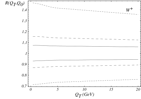
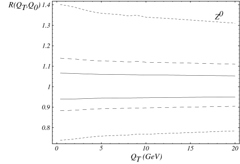
FIG. 3.: The ratio $R(Q_{T},Q_{0})$, with $y_{0}=0$, for $W^{+}$ and $Z^{0}$ bosons as a function of $Q_{T}$. For $W^{+}$, solid lines are: $Q_{0}=78$ GeV (upper) and 82 GeV (lower), dashed: $Q_{0}=76$ GeV (upper) and 84 GeV (lower), dotted: $Q_{0}=70$ GeV (upper) and 90 GeV (lower). For $Z^{0}$ bosons, solid lines: $Q_{0}=88$ GeV (upper) and 92 GeV (lower), dashed: $Q_{0}=86$ GeV (upper) and 94 GeV (lower), dotted: $Q_{0}=80$ GeV (upper) and 100 GeV (lower).

Similarly, we define the ratio

$$R(Q_{T},y_{0})={\frac{\left.\displaystyle\frac{d\sigma}{dQ^{2}dQ_{T}^{2}dy}\right|_{Q=M_{V},y=y_{0}}}{\left.\displaystyle\frac{d\sigma}{dQ^{2}dQ_{T}^{2}dy}\right|_{Q=M_{V},y=0}}},$$

to study the $Q_{T}$ shape variation as a function of the vector boson rapidity. Our results are shown in Fig. 4. Unlike the ratio $R(Q_{T},Q_{0})$ shown in Fig. 3, the distributions of $R(Q_{T},y_{0})$ for the $W^{\pm}$ and $Z^{0}$ bosons are clearly different for any value of the rapidity $y_{0}$.

To utilize the information on the transverse momentum of the $W^{+}$ boson in Monte Carlo simulations to reconstruct the mass of the $W^{+}$ boson, it was suggested in Ref. [25] to predict $Q_{T}(W^{+})$ distribution from the measured $Q_{T}(Z^{0})$ distribution and the calculated ratio of $Q_{T}(W^{+})$ and $Q_{T}(Z^{0})$ predicted by the resummation calculations [7, 12], in which the vector boson is assumed to be on its mass-shell. Unfortunately, this idea will not work with a good precision because, as clearly shown in Fig. 4, the ratio of the $W^{+}$ and $Z^{0}$ transverse momentum distributions depends on the rapidities of the vector bosons. Since the rapidity of the $W^{+}$ boson cannot be accurately reconstructed without knowing the longitudinal momentum (along the beam pipe direction) of the neutrino, which is in the form of missing energy carried away by the neutrino, this dependence cannot be incorporated in data analysis and the above ansatz cannot be realized in practice for a precision measurement of $M_{W}$. Only the Monte Carlo implementation of the exact matrix element calculation (ResBos) can correctly predict the distributions of the decay leptons, such as the transverse mass of the $W^{\pm}$ boson, and the transverse momentum of the charged lepton, so that they can be directly compared with experimental data to extract the value of $M_{W}$. We comment on these results later in this section.

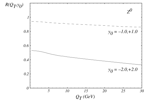
FIG. 4.: The ratio $R(Q_{T},y_{0})$, with $Q_{0}=M_{V}$, for $W^{+}$ and $Z^{0}$ bosons as a function of $Q_{T}$.

Another way to compare the results of the resummed and the NLO calculations is given by the distributions of $\sigma(Q_{T}>Q_{T}^{\min})/\sigma_{Total}$, as shown in Fig. 5. We defined the ratio as

$\displaystyle R_{CSS}\equiv\frac{\sigma(Q_{T}>Q_{T}^{\min})}{\sigma_{Total}}=\frac{1}{\sigma_{Total}}\int_{Q_{T}^{\min}}^{Q_{T}^{\max}}dQ_{T}\;\frac{d\sigma(h_{1}h_{2}\rightarrow V)}{dQ_{T}},$where $Q_{T}^{\max}$ is the largest $Q_{T}$ allowed by the phase space. In the NLO calculation, $\sigma(Q_{T}>Q_{T}^{\min})$ grows without bound near $Q_{T}^{\min}=0$, as the result of the singular behavior $1/Q_{T}^{2}$ in the matrix element. The NLO curve runs well under the resummed one in the 2 GeV $<Q_{T}^{\min}<$ 30 GeV region, and the $Q_{T}$ distributions from the NLO and the resummed calculations have different shapes even in the region where $Q_{T}$ is of the order 15 GeV.

With large number of fully reconstructed $Z^{0}$ events at the Tevatron, one should be able to use data to discriminate these two theory calculations. In view of this result it is not surprising that the DØ  analysis of the $\alpha_{S}$ measurement [26] based on the measurement of $\sigma(W+1\;jet)/\sigma(W+0\;jet)$ does not support the NLO calculation in which the effects of the multiple gluon radiation are not included. We expect that if this measurement was performed by demanding the transverse momentum of the jet to be larger than about 50 GeV, at which scale the resummed and the NLO distributions in Fig. 2 cross, the NLO calculation would adequately describe the data.

FIG. 5.: The ratio $R_{CSS}$ as a function of $Q_{T}^{\min}$ for $W^{+}$ and $Z^{0}$ bosons. The fixed order (${\cal O}(\alpha_{S})$ short dashed, ${\cal O}(\alpha_{S}^{2})$ dashed) curves are ill-defined in the low $Q_{T}$ region. The resummed (solid) curves are calculated for $g_{2}$ = 0.38 (low), 0.58 (middle) and 0.68 (high) GeV² values.

To show that for $Q_{T}$ below 30 GeV, the QCD multiple soft gluon radiation is important to explain the DØ  data [26], we also include in Fig. 5 the prediction for the $Q_{T}$ distribution at the order of $\alpha^{2}_{S}$. As shown in the figure, the $\alpha^{2}_{S}$ curve is closer to the resummed curve which proves that for this range of $Q_{T}$ the soft gluon effect included in the $\alpha^{2}_{S}$ calculation is important for predicting the vector boson $Q_{T}$ distribution. In other words, in this range of $Q_{T}$, it is more likely that soft gluons accompany the $W^{\pm}$ boson than just a single hard jet associated with the vector boson production. For large $Q_{T}$, it becomes more likely to have hard jet(s) produced with the vector boson.

Measuring $R_{CSS}$ in the low $Q_{T}$ region (for $Q_{T}\lesssim Q/2$) provides a stringent test of the dynamics of the multiple soft gluon radiation predicted by the QCD theory. The same measurement of $R_{CSS}$ can also provide information about some part of the non-perturbative physics associated with the initial state hadrons. As shown in Fig. 6 and in Ref. [22], the effect of the non-perturbative physics on the $Q_{T}$ distributions of the $W^{\pm}$ and $Z^{0}$ bosons produced at the Tevatron is important for $Q_{T}$ less than about 10 GeV. This is evident by observing that different parametrizations of the non-perturbative functions do not change the $Q_{T}$ distribution for $Q_{T}>10$ GeV, although they do dramatically change the shape of $Q_{T}$ for $Q_{T}<10$ GeV. Since for $W^{\pm}$ and $Z^{0}$ production, the $\ln(Q^{2}/Q^{2}_{0})$ term is large, the non-perturbative function, as defined in Eq. (12), is dominated by the $F_{1}(b)$ term (or the $g_{2}$ parameter) which is supposed to be universal for all Drell-Yan type processes and related to the physics of the renormalon [20]. Hence, the measurement of $R_{CSS}$ cannot only be used to test the dynamics of the QCD multiple soft gluon radiation, in the $10\,{\rm GeV}\,<Q_{T}<40$ GeV region, but may also be used to probe this part of non-perturbative physics for $Q_{T}<10$ GeV. It is therefore important to measure $R_{CSS}$ at the Tevatron. With a large sample of $Z^{0}$ data at Run 2, it is possible to determine the dominant non-perturbative function which can then be used to calculate the $W^{\pm}$ boson $Q_{T}$ distribution to improve the accuracy of the $M_{W}$ and the charged lepton rapidity asymmetry measurements.

FIG. 6.: Transverse momentum distributions of $W^{+}$ and $Z^{0}$ bosons calculated with low (long dash, $g_{2}$ = 0.38 GeV²), nominal (solid, $g_{2}$ = 0.58 GeV²) and high (short dash, $g_{2}$ = 0.68 GeV²) $g_{2}$ non-perturbative parameter values. The low and high excursions in $g_{2}$ are the present one standard deviations from the nominal value in the Ladinsky-Yuan parametrization.

B The Total Cross Section

Before we compare the distributions of the decay leptons, we examine the question whether or not the $Q_{T}$ resummation formalism changes the prediction for the total cross section. In Ref. [27] it was shown that in the AEGM formalism, which differs from the CSS formalism, the ${\cal O}(\alpha_{S})$ total cross section is obtained after integrating their resummation formula over the whole range of the phase space.

In the CSS formalism, without including the $C$ and $Y$ functions, the fully integrated resummed result recovers the ${\cal O}(\alpha_{S}^{0})$ cross section, provided that $Q_{T}$ is integrated from zero to $Q$. This can be easily verified by expanding the resummation formula up to ${\cal O}(\alpha_{S})$, dropping the $C^{(1)}$ and the $Y$ pieces (which are of order ${\cal O}(\alpha_{S})$), and integrating over the lepton variables. It yields

$$\int_{0}^{P_{T}^{2}}dQ_{T}^{2}\;\frac{d\sigma}{dQ^{2}dydQ_{T}^{2}}=\frac{\sigma_{0}}{S}\delta(Q^{2}-M_{V}^{2})$$ (19)

$$\ \ \ \ \ \times\left\{\left(1-\frac{\alpha_{S}(Q)}{\pi}\left[\frac{1}{2}A^{(1)}\ln^{2}\left(\frac{Q^{2}}{P_{T}^{2}}\right)+B^{(1)}\ln\left(\frac{Q^{2}}{P_{T}^{2}}\right)\right]\right)\;f_{j/h_{1}}(x_{1},Q^{2})\;f_{\overline{k}/h_{2}}(x_{2},Q^{2})\right.$$

$$\ \ \ \ \ -\frac{\alpha_{S}(Q)}{2\pi}\ln\left(\frac{Q^{2}}{P_{T}^{2}}\right)\left[\left(P_{j\leftarrow a}\otimes f_{a/h_{1}}\right)(x_{1},Q^{2})\;f_{\overline{k}/h_{2}}(x_{2},Q^{2})\right.$$

$$~{}~{}~{}~{}~{}~{}~{}~{}~{}~{}~{}~{}~{}~{}~{}~{}~{}~{}~{}~{}~{}~{}~{}~{}~{}~{}~{}\left.\left.+\;f_{j/h_{1}}(x_{1},Q^{2})\left(P_{\overline{k}\leftarrow b}\otimes f_{b/h_{2}}\right)(x_{2},Q^{2})\right]+j\leftrightarrow\overline{k}\right\},$$

where $P_{T}$ is the upper limit of the $Q_{T}$ integral and we fixed the mass of the vector boson for simplicity. To derive the above result we have used the canonical set of the $C_{i}$ ($i=1,2,3$) coefficients (cf. Appendix C and D). When the upper limit $P_{T}$ is taken to be $Q$, all the logs in the above equation vanish and Eq. (19) reproduces the Born level (${\cal O}(\alpha_{S}^{0})$) cross section. Similar conclusion holds for higher order terms from the expansion of the resummed piece when $C$ and $Y$ are not included. This is evident because the singular pieces from the expansion are given by

$$\left.\frac{d\sigma}{dQ_{T}^{2}}\right|_{singular}=\frac{1}{Q_{T}^{2}}\sum_{n=1}^{\infty}\sum_{m=0}^{2n-1}{}_{n}v_{m}\alpha_{S}^{n}\ln^{m}\left(\frac{Q_{T}^{2}}{Q^{2}}\right)$$

The integral of these singular terms will be proportional to $\ln(Q^{2}/P_{T}^{2})$ raised to some power. Again, for $P_{T}=Q$ all the logs vanish and the tree level result is obtained.

The inclusion of $C^{(1)}$ and $Y$ functions will change the above conclusion and lead to a different total cross section, because $C^{(1)}$ contains the hard part virtual corrections and $Y$ contains the hard gluon radiation. In the $Q_{T}<Q$ region the resummed piece dominates, because it resums the singular pieces: $Q_{T}^{-2}\times[1$ or $\ln(Q^{2}/Q_{T}^{2})]$, to all order. However, in the $Q_{T}>Q$ region the perturbative result should be used, because the singular pieces do not dominate (the logs are small in this case) and the other contributions in the fixed order perturbative contributions can be important. In order to define the total cross section a prescription of smooth transition between the resummed and the fixed order perturbative results is necessary. In Fig. 2, we show the resummed (1,1) (resummation with $A^{(1)},B^{(1)}$ and $C^{(0,1)}$ included) and the fixed order ${\cal O}(\alpha_{S})$ $Q_{T}$ distributions for $W^{+}$ and $Z^{0}$ bosons. As shown, the resummed (1,1) and the fixed order curves are close to each other for $Q/2<Q_{T}<Q$, and they cross near $Q_{T}\sim Q/2$. Henceforth, we adopt the following matching procedure. For $Q_{T}$ values below the crossing point we use the resummed curve, and above it the ${\cal O}(\alpha_{S})$ curve, to define a resummed ${\cal O}(\alpha_{S})$ distribution. This distribution is smooth (although not differentiable at the matching point), and most importantly it does not alter either the resummed or the ${\cal O}(\alpha_{S})$ distributions in the kinematic regions where they are proven to be valid. This simple matching prescription provides us with an ${\cal O}(\alpha_{S})$ resummed total cross section with an error of ${\cal O}(\alpha_{s}^{2})$, as shown in Ref. [12]. In practice this translates into less than a percent deviation between the fixed order and the resummed ${\cal O}(\alpha_{S})$ total cross sections. This can be understood from the earlier discussion that if the matching were done at $Q_{T}$ equal to $Q$, then the total cross section calculated from the CSS resummation formalism should be the same as that predicted by the NLO calculation, provided that $C^{(1)}$ and $Y^{(1)}$ are included. However, this matching prescription would not result in a smooth curve for the $Q_{T}$ distribution at $Q_{T}=Q$. The small difference between the resummed ${\cal O}(\alpha_{S})$ and the NLO [fixed order, ${\cal O}(\alpha_{S})$] total cross sections comes from the matching procedure described above. This difference indicates the size of the higher order corrections not included in the NLO calculation.

In order to compare the $Q_{T}$ distribution with experimental data we also include the effect of some known higher order corrections to the Sudakov factor and plot the resummed (2,1) (with $A^{(1,2)},B^{(1,2)}$ and $C^{(0,1)}$ included) and the fixed order ${\cal O}(\alpha_{S}^{2})$ distributions [28]. We match the two distributions at the value of $Q_{T}$, about 48 GeV, where they cross over for $W^{+}$ production, that defines the resummed ${\cal O}(\alpha_{S}^{2})$ distribution in the whole $Q_{T}$ region. The total cross section predicted from various theory calculations are listed in Table III.

$V$	$E_{cm}$	Fixed Order		CSS (1,1) + Y	CSS (2,1) + Y		Experiment
	(TeV)	${\cal O}(\alpha_{S}^{0})$	${{\cal O}(\alpha_{S})}$	$\oplus$ Pert. ${\cal O}(\alpha_{S})$	$\oplus$ Pert. ${\cal O}(\alpha_{S})$	$\oplus$ Pert. ${\cal O}(\alpha_{S}^{2})$	(Ref. [45])
W+	1.8	8.81	11.1	11.3	11.3	11.4	11.5 $\pm$ 0.7
W+	2.0	9.71	12.5	12.6	12.6	12.7
Z0	1.8	5.23	6.69	6.79	6.79	6.82	6.86 $\pm$ 0.36
Z0	2.0	6.11	7.47	7.52	7.52	7.57

TABLE III.: Total cross sections of $p{\bar{p}}\rightarrow(W^{+}{\rm or}~{}Z^{0})X$ at the present and upgraded Tevatron, calculated in different prescriptions, in units of nb. The finite order total cross section results are based on the calculations in Ref. [27]. The Pert. ${\cal O}(\alpha_{S}^{2})$ results were obtained from Ref. [28]. The “$+$” signs refer to the inclusion of the $Y$ piece and the “$\oplus$” signs to the switch from the resummed to the fixed order calculations.

We note that kinematic cuts affect the total cross section in a subtle manner. It is obvious from our matching prescription that the resummed ${\cal O}(\alpha_{S}^{2})$ and the fixed order ${\cal O}(\alpha_{S})$ curves in Fig. 2 will never cross. On the other hand, the resummed ${\cal O}(\alpha_{S}^{2})$ total cross section is about the same as the fixed order ${\cal O}(\alpha_{S})$ cross section when integrating $Q_{T}$ from 0 to $Q$. These two facts imply that when kinematic cuts are made on the $Q_{T}$ distribution with $Q_{T}<Q$, we will obtain a higher total cross section in the fixed order ${\cal O}(\alpha_{S})$ than in the resummed ${\cal O}(\alpha_{S}^{2})$ calculation. In this paper we follow the CDF cuts (for the $W^{+}$ boson mass analysis) and demand $Q_{T}<30$ GeV [46]. Consequently, in many of our figures, to be shown below, the fixed order ${\cal O}(\alpha_{S})$ curves give about 3% higher total cross section than the resummed ones.

C Lepton Charge Asymmetry

The CDF lepton charge asymmetry measurement [29] played a crucial role in constraining the slope of the $u/d$ ratio in recent parton distribution functions. It was shown that one of the largest theoretical uncertainty in the $W^{\pm}$ mass measurement comes from the parton distributions [30], and the lepton charge asymmetry was shown to be correlated with the transverse mass distribution [31]. Among others, the lepton charge asymmetry is studied to decrease the errors in the measurement of $M_{W}$ coming from the parton distributions. Here we investigate the effect of the resummation on the lepton rapidity distribution, although it is not one of those observables which are most sensitive to the $Q_{T}$ resummation, i.e. to the effect of multiple soft gluon radiation.

The definition of the charge asymmetry is

$$A(y)=\frac{\displaystyle\frac{d\sigma}{dy_{+}}-\frac{d\sigma}{dy_{-}}}{\displaystyle\frac{d\sigma}{dy_{+}}+\frac{d\sigma}{dy_{-}}},$$

where $y_{+}$ ($y_{-}$) is the rapidity of the positively (negatively) charged particle (either vector boson or decay lepton). Assuming CP invariance, the following relation holds:

$${\frac{d\sigma}{dy_{+}}}(y)={\frac{d\sigma}{dy_{-}}}(-y).$$

Hence, the charge asymmetry is frequently written as

$$A(y)=\frac{\displaystyle\frac{d\sigma}{dy}(y>0)-\frac{d\sigma}{dy}(y<0)}{\displaystyle\frac{d\sigma}{dy}(y>0)+\frac{d\sigma}{dy}(y<0)}.$$

For the charge asymmetry of the vector boson ($W^{\pm}$) or the charged decay lepton ($\ell^{\pm}$), the fixed order and the resummed ${\cal O}(\alpha_{S})$ [or ${\cal O}(\alpha_{S}^{2})$] results are the same, provided that there are no kinematic cuts imposed. This is because the shape difference in the vector boson transverse momentum has been integrated out and the total cross sections are the same up to higher order corrections in $(\alpha_{S})$. In Fig. 7(a) we show the lepton charge asymmetry without cuts for CTEQ4M PDF. The NLO and the resummed curves overlap, although they differ from the ${\cal O}(\alpha_{S}^{0})$ prediction.

FIG. 7.: Lepton charge asymmetry distributions. (a) Without any kinematic cuts, the NLO (long dashed) and the resummed ${\cal O}(\alpha_{S})$ (solid) curves overlap and the LO (short dashed) curve differs somewhat from them. (b) With cuts ($Q_{T}<30~{}{\rm GeV},p_{T}^{e^{+},\nu}>25~{}{\rm GeV}$), the effect of the different $Q_{T}$ distributions renders the lepton rapidity asymmetry distributions different. The two resummed curves calculated with $g_{2}$ = 0.58 and 0.78 GeV^-2 cannot be distinguished on this plot.

On the other hand, when kinematic cuts are applied to the decay leptons, the rapidity distributions of the vector bosons or the leptons in the fixed order and the resummed calculations are different. Restriction of the phase space implies that only part of the vector boson transverse momentum distribution is sampled. The difference in the resummed and the fixed order $Q_{T}$ distributions will prevail as a difference in the rapidity distributions of the charged lepton. We can view this phenomenon in a different (a Monte Carlo) way. In the rest frame of the $W^{\pm}$, the decay kinematics is the same, whether it is calculated up to ${\cal O}(\alpha_{S})$ or within the resummation formalism. On the other hand, the $W^{\pm}$ rest frame is different for each individual Monte Carlo (MC) event depending on the order of the calculation. This difference is caused by the fact that the $Q_{T}$ distribution of the $W^{\pm}$ is different in the ${\cal O}(\alpha_{S})$ and the resummed calculations, and the kinematic cuts select different events in these two cases. Hence, even though the $Q_{T}$ distribution of the $W^{\pm}$ is integrated out, when calculating the lepton rapidity distribution, we obtain slightly different predictions in the two calculations. The difference is larger for larger $|y^{\ell}|$, being closer to the edge of the phase space, because the soft gluon radiation gives high corrections there and this effect up to all order in $\alpha_{S}$ is contained in the resummed but only up to order of $\alpha_{S}$ in the NLO calculation. Because the rapidity of the lepton and that of the vector boson are highly correlated, large rapidity leptons mostly come from large rapidity vector bosons. Also, a vector boson with large rapidity tends to have low transverse momentum, because the available phase space is limited to low $Q_{T}$ for a $W^{\pm}$ boson with large $|y|$. Hence, the difference in the low $Q_{T}$ distributions of the NLO and the resummed calculations yields the difference in the $y^{\ell}$ distribution for leptons with high rapidities.

Asymmetry distributions of the charged lepton with cuts using the CTEQ4M PDF are shown in Fig. 7(b). The applied kinematic cuts are: $Q_{T}<30$ GeV, $p_{T}^{e^{+},\nu}>25$. These are the cuts that CDF used when extracted the lepton rapidity distribution from their data [29]. We have checked that the ResBos fixed order ${\cal O}(\alpha_{S})$ curve agrees well with the DYRAD [24] result. As anticipated, the ${\cal O}(\alpha_{S}^{0})$, ${\cal O}(\alpha_{S})$ and resummed results deviate at higher rapidities ($|y^{e}|>1.5$). The deviation between the NLO and the resummed curves indicates that to extract information on the PDF in the large rapidity region, the resummed calculation, in principle, has to be used if the precision of the data is high enough to distinguish these predictions. Fig. 7(b) also shows the negligible dependence of the resummed curves on the non-perturbative parameter $g_{2}$. We plot the result of the resummed calculations with the nominal $g_{2}$ = 0.58 GeV^-2, and with $g_{2}$ = 0.78 GeV^-2 which is two standard deviations higher. The deviation between these two curves (which is hardly observable on the figure) is much smaller than the deviation between the resummed and the NLO ones.

There is yet another reason why the lepton charge asymmetry can be reliably predicted only by the resummed calculation. When calculating the lepton distributions in a numerical ${\cal O}(\alpha_{S})$ code, one has to artificially divide the vector boson phase space into hard and soft regions, depending on – for example – the energy or the $Q_{T}$ of the emitted gluon (e.g. $q\overline{q}\rightarrow W+\;$hard or soft gluon). The observables calculated with this phase space slicing technique acquire a dependence on the scale which separates the hard from the soft regions. To emphasize this dependence as an example, we show that when the phase space is divided by the $Q_{T}$ separation, the dependence of the asymmetry on the scale $Q_{T}^{Sep}$ can be comparable to the difference in the ${\cal O}(\alpha_{S})$ and the resummed results. This means that there is no definite prediction from the NLO calculation for the lepton rapidity distribution. Only the resummed calculation can give an unambiguous prediction for the lepton charge asymmetry.

Before closing this section, we also note that although in the lepton asymmetry distribution the NLO and resummed results are about the same for $|y^{e^{+}}|<1$, it does not imply that the rapidity distributions of the leptons predicted by those two theory models are the same. As shown in Fig. 8, this difference can in principle be observable with a large statistics data sample and a good knowledge of the luminosity of the colliding beams.

FIG. 8.: Distributions of positron rapidities from the decays of $W^{+}$’s produced at the Tevatron, predicted by the resummed (solid) and the NLO (dashed) calculations with the same kinematic cuts as for the asymmetry plot.

D Transverse Mass Distribution

Since the invariant mass of the $W^{\pm}$ boson cannot be reconstructed without knowing the longitudinal momentum of the neutrino, one has to find a quantity that allows an indirect determination of the mass of the $W^{\pm}$ boson. In the discovery stage of the $W^{\pm}$ bosons at the CERN ${\rm Sp\overline{p}S}$ collider, the mass and width were measured using the transverse mass distribution of the charged lepton-neutrino pair from the $W^{\pm}$ boson decay. Ever since the early eighties, the transverse mass distribution, $m_{T}=\sqrt{2p_{T}^{e}p_{T}^{\nu}(1-\cos\Delta\phi_{e\nu})}$, has been known as the best measurable for the extraction of both $M_{W}$ and $\Gamma_{W}$, for it is insensitive to the transverse momentum of the $W^{\pm}$ boson. The effect of the non-vanishing vector boson transverse momentum on the $m_{T}$ distribution was analyzed  [32, 33] well before the $Q_{T}$ distribution of the $W^{\pm}$ boson was correctly calculated by taking into account the multiple soft gluon radiation. Giving an average transverse boost to the vector boson, the authors of Ref. [32] concluded that for the fictive case of $\Gamma_{W}$ = 0, the end points of the transverse mass distribution are fixed at zero: $d\sigma/dm_{T}^{2}(m_{T}^{2}=0)=d\sigma/dm_{T}^{2}(m_{T}^{2}=M_{W}^{2})=0$. The sensitivity of the $m_{T}$ shape to a non-zero $Q_{T}$ is in the order of $\left\langle(Q_{T}/M_{W})^{2}\right\rangle\approx$1% without affecting the end points of the $m_{T}$ distribution. Including the effect of the finite width of the $W^{\pm}$ boson, the authors in Ref. [33] showed that the shape and the location of the Jacobian peak are not sensitive to the $Q_{T}$ of the $W^{\pm}$ boson either. The non-vanishing transverse momentum of the $W^{\pm}$ boson only significantly modifies the $m_{T}$ distribution around $m_{T}=0$.

Our results confirm that the shape of the Jacobian peak is quite insensitive to the order of the calculation. We show the NLO and the resummed transverse mass distributions in Fig. 9 for $W^{\pm}$ bosons produced at the Tevatron with the kinematic cuts: $Q_{T}<30$ GeV, $p_{T}^{e^{+},\nu}>25$ GeV and $|y^{e^{+}}|<3.0$. Fig. 9(a) covers the full (experimentally interesting) $m_{T}$ range while Fig. 9(b) focuses on the $m_{T}$ range which contains most of the information about the $W^{\pm}$ mass. There is little visible difference between the $shapes$ of the NLO and the resummed $m_{T}$ distributions. On the other hand, the right shoulder of the curve appears to be “shifted” by about 50 MeV, because, as noted in Section III B, the total cross sections are different after the above cuts imposed in the NLO and the resummed calculations. At Run 2 of the Tevatron, with large integrated luminosity ($\sim 2~{}{\rm fb}^{-1}$), the goal is to extract the $W^{\pm}$ boson mass with a precision of 30-50 MeV from the $m_{T}$ distribution [30]. Since $M_{W}$ is sensitive to the position of the Jacobian peak [33], the high precision measurement of the $W^{\pm}$ mass has to rely on the resummed calculations.

FIG. 9.: Transverse mass distribution for $W^{+}$ production and decay at the 1.8 TeV Tevatron.

Extraction of $M_{W}$ from the transverse mass distribution has some drawbacks though. The reconstruction of the transverse momentum $p_{T}^{\nu}$ of the neutrino involves the measurement of the underlying event transverse momenta: $\vec{p}_{T}^{~{}\nu}=-\vec{p}_{T}^{~{}\ell}-\vec{p}_{T}^{~{}recoil}-\vec{p}_{T}^{~{}underlying~{}event}$. This resolution degrades by the number of interactions per crossing ($N_{I_{c}}$) [30]. With a high luminosity ($\sim 100\,{\rm fb}^{-1}$) at the 2 TeV Tevatron (TEV33) [34], $N_{I_{c}}$ can be as large as 10, so that the Jacobian peak is badly smeared. This will lead to a large uncertainty in the measurement of $M_{W}$. For this reason the systematic precision of the $m_{T}$ reconstruction will be less at the high luminosity Tevatron, and an $M_{W}$ measurement that relies on the lepton transverse momentum distribution alone could be more promising. We discuss this further in the next section.

The theoretical limitation on the $M_{W}$ measurement using the $m_{T}$ distribution comes from the dependence on the non-perturbative sector, i.e. from the PDF’s and the non-perturbative parameters in the resummed formalism. Assuming the PDF’s and these non-perturbative parameters to be independent variables, the uncertainties introduced are estimated to be less than 50 MeV and 10 MeV, respectively, at the TEV33 [36, 37]. It is clear that the main theoretical uncertainty comes from the PDF’s. As to the uncertainty due to the non-perturbative parameters (e.g. $g_{2}$) in the CSS resummation formalism, it can be greatly reduced by carefully study the $Q_{T}$ distribution of the $Z^{0}$ boson which is expected to be copiously produced at Run 2 and beyond.

The $M_{W}$ measurement at the LHC may also be promising. Both ATLAS and CMS detectors are well optimized for measuring the leptons and the missing $E_{T}$ [37]. The cross section of the $W^{+}$ boson production is about four times larger than that at the Tevatron, and in one year of running with 20 fb^-1 luminosity yields a few times $10^{7}$ $W\rightarrow\ell\nu$ events after imposing similar cuts to those made at the Tevatron. Since the number of interactions per crossing may be significantly lower (in average $N_{I_{c}}$ = 2) at the same or higher luminosity than that at the TEV33 [37], the Jacobian peak in the $m_{T}$ distribution will be less smeared at the LHC than at the TEV33. Furthermore, the non-perturbative effects are relatively smaller at the LHC because the perturbative Sudakov factor dominates. On the other hand, the probed region of the PDF’s at the LHC has a lower value of the average $x~{}(\sim 10^{-3})$ than that at the Tevatron $(\sim 10^{-2})$, hence the uncertainty from the PDF’s might be somewhat larger. A more detailed study of this subject is desirable.

E Lepton Transverse Momentum

Due to the limitations mentioned above, the transverse mass ($m_{T}$) method may not be the only and the most promising way for the precision measurement of $M_{W}$ at some future hadron colliders. As discussed above, the observable $m_{T}$ was used because of its insensitivity to the high order QCD corrections. In contrast, the lepton transverse momentum ($p_{T}^{\ell}$) distribution receives a large, ${\cal O}\left(\left\langle Q_{T}/M_{W}\right\rangle\right)\sim 10\%$perturbative QCD correction at the order $\alpha_{S}$, as compared to the Born process. With the resummed results in hand it becomes possible to calculate the $p_{T}^{\ell}$ distribution precisely within the perturbative framework, and to extract the $W^{\pm}$ mass straightly from the transverse momentum distributions of the decay leptons.

Just like in the $m_{T}$ distribution, the mass of the $W^{\pm}$ boson is mainly determined by the shape of the distribution near the Jacobian peak. The location of the maximum of the peak is directly related to the $W^{\pm}$ boson mass, while the theoretical width of the peak varies with its decay width $\Gamma_{W}$. Since the Jacobian peak is modified by effects of both $Q_{T}$ and $\Gamma_{W}$, it is important to take into account both of these effects correctly. In our calculation (and in ResBos) we have properly included both effects.

The effect of resummation on the transverse momentum distribution of the charged lepton from $W^{+}$ and $Z^{0}$ decays is shown in Fig. 10. The NLO and the resummed distributions differ a great amount even without imposing any kinematic cuts. The clear and sharp Jacobian peak of the NLO distribution is strongly smeared by the finite transverse momentum of the vector boson introduced by multiple gluon radiation. This higher order effect cannot be correctly calculated in any finite order of the perturbation theory and the resummation formalism has to be used.

FIG. 10.: Transverse momentum distributions of $p_{T}^{e^{+}}$ from $W^{+}$ and $Z^{0}$ decays for the NLO (dashed) and the resummed ${\cal O}(\alpha_{S})$ (solid) calculations. Resumming the initial state multiple soft-gluon emission has the typical effect of smoothening and broadening the Jacobian peak (at $p_{T}^{e^{+}}=M_{V}/2$). The CDF cuts are imposed on the $W^{+}$ distributions, but there are no cuts on the $Z^{0}$ distributions.

One of the advantages of using the $p_{T}^{\ell}$ distribution to determine $M_{W}$ is that there is no need to reconstruct the $p_{T}^{\nu}$ distribution which potentially limits the precision of the $m_{T}$ method. From the theoretical side, the limitation is in the knowledge of the non-perturbative sector. Studies at DØ  [35] show that the $p_{T}^{\ell}$ distribution is most sensitive to the PDF’s and the value of the non-perturbative parameter $g_{2}$. The $p_{T}^{\ell}$ distribution is more sensitive to the PDF choice, than the $m_{T}$ distribution is. The uncertainty in the PDF causes an uncertainty in $M_{W}$ of about 150 MeV, which is about three times as large as that using the $m_{T}$ method [35]. A 0.1 GeV² uncertainty in $g_{2}$ leads to about $\Delta M_{W}=30$ MeV uncertainty from the $p_{T}^{\ell}$ fit, which is about five times worse than that from the $m_{T}$ measurement [35]. Therefore, to improve the $M_{W}$ measurement, it is necessary to include the $Z^{0}$ data sample at the high luminosity Tevatron to refit the $g_{i}$’s and obtain a tighter constrain on them from the $Q_{T}$ distribution of the $Z^{0}$ boson. The DØ  study showed that an accuracy of $\Delta g_{2}=0.01$ GeV² can be achieved with Run 2 and TeV33 data, which would contribute an error of $\Delta M_{W}<5$ MeV from the $p_{T}^{\ell}$ [35]. In this case the uncertainty coming from the PDF’s remains to be the major theoretical limitation. At the LHC, the $p_{T}^{\ell}$ distribution can be predicted with an even smaller theoretical error coming from the non-perturbative part, because at higher energies the perturbative Sudakov factor dominates over the non-perturbative function.

It was recently suggested to extract $M_{W}$ from the ratios of the transverse momenta of leptons produced in $W^{\pm}$ and $Z^{0}$ decay [38]. The theoretical advantage is that the non-perturbative uncertainties are decreased in such a ratio. On the other hand, it is not enough that the ratio of cross sections is calculated with small theoretical errors. For a precision extraction of the $W^{\pm}$ mass the theoretical calculation must be capable of reproducing the individually observed transverse momentum distributions themselves. The $W^{\pm}$ mass measurement requires a detailed event modeling, understanding of detector resolution, kinematical acceptance and efficiency effects, which are different for the $W^{\pm}$ and $Z^{0}$ events, as illustrated above. Therefore, the ratio of cross sections can only provide a useful check for the $W^{\pm}$ mass measurement.

For Drell-Yan events or lepton pairs from $Z^{0}$ decays, additional measurable quantities can be constructed from the lepton transverse momenta. They are the distributions in the balance of the transverse momenta $(\Delta{p}_{T}=|{\vec{p}}_{T}^{\,\ell_{1}}|-|{\vec{p}}_{T}^{\,{\bar{\ell}_{2}}}|)$ and the angular correlation of the two lepton momenta $({z=-\vec{p}}_{T}^{\,\ell_{1}}\cdot{\vec{p}}_{T}^{\,{\bar{\ell}_{2}}}/[\max(p_{T}^{\,\ell_{1}},p_{T}^{\,{\bar{\ell}_{2}}})]^{2})$. It is expected that these quantities are also sensitive to the effects of the multiple soft gluon radiation. These distributions are shown in Figure 11. As shown, the resummed distributions significantly differ from the NLO ones. In these, and the following figures for $Z^{0}$ decay distributions, it is understood that the following kinematic cuts are imposed: $Q_{T}^{Z^{0}}<30$ GeV, $p_{T}^{e^{+},e^{-}}>25$ GeV and $|y^{e^{+},e^{-}}|<3.0$, unless indicated otherwise.

FIG. 11.: Balance in transverse momentum $\Delta{p}_{T}=|{\vec{p}}_{T}^{\,\ell_{1}}|-|{\vec{p}}_{T}^{\,{\bar{\ell}_{2}}}|$ and angular correlation ${z=-\vec{p}}_{T}^{\,\ell_{1}}\cdot{\vec{p}}_{T}^{\,{\bar{\ell}_{2}}}/[\max(p_{T}^{\ell_{1}},p_{T}^{{\bar{\ell}_{2}}})]^{2}$ of the decay leptons from $Z^{0}$ bosons produced at the Tevatron.

F Lepton Angular Correlations

Another observable that can serve to test the QCD theory beyond the fixed-order perturbative calculation is the difference in the azimuthal angles of the leptons $\ell_{1}$ and ${\bar{\ell}_{2}}$ from the decay of a vector boson $V$. In practice, this can be measured for $\gamma^{*}\text{ or }Z^{0}\rightarrow\ell_{1}{\bar{\ell}_{2}}$. We show in Fig. 12 the difference in the azimuthal angles of $e^{+}$ and $e^{-}$ ($\Delta\phi^{e^{+}e^{-}}$), measured in the laboratory frame for $Z^{0}\rightarrow e^{+}e^{-}$, calculated in the NLO and the resummed approaches. As indicated, the NLO result is ill-defined in the vicinity of $\Delta\phi\sim\pi$, where the multiple soft-gluon radiation has to be resummed to obtain physical predictions.

FIG. 12.: The correlation between the lepton azimuthal angles near the region $\Delta\phi\sim\pi$ for $p{\bar{p}}\rightarrow(Z^{0}\rightarrow e^{+}e^{-})X$. The resummed (solid) distribution gives the correct angular correlation of the lepton pair. The NLO (dashed lines) distribution near $\Delta\phi=\pi$ is ill-defined and depends on $Q_{T}^{Sep}$ (the scale for separating soft and hard gluons in the NLO calculation). The two NLO distributions were calculated with $Q_{T}^{Sep}=1.2$ GeV (long dash) and $Q_{T}^{Sep}=2.0$ GeV (short dash).

Another interesting angular variable is the lepton polar angle distribution $\cos\theta^{*\ell}$ in the Collins-Soper frame. It can be calculated for the $Z^{0}$ decay and used to extract $\sin^{2}\theta_{w}$ at the Tevatron [39]. The asymmetry in the polar angle distribution is essentially the same as the forward-backward asymmetry $A_{FB}$ measured at LEP. Since $A_{FB}$ depends on the invariant mass $Q$ and around the energy of the $Z^{0}$ peak $A_{FB}$ happens to be very small, the measurement is quite challenging. At the hadron collider, on the other hand, the invariant mass of the incoming partons is distributed over a range so the asymmetry is enhanced [15]. The potentials of the measurement deserve a separated study. In Fig. 13 we show the distributions of $\cos\theta^{*\ell}$ predicted from the NLO and the resummed results.

FIG. 13.: Distribution of the $e^{+}$ polar angle $\cos(\theta^{*})$ in the Collins-Soper frame from $Z^{0}$ decays at the Tevatron with cuts indicated in the text.

G Vector Boson Longitudinal Distributions

The resummation of the logs involving the transverse momentum of the vector boson does not directly affect the shape of the longitudinal distributions of the vector bosons. A good example of this is the distribution of the longitudinal momentum of the $Z^{0}$ boson which can be measured at the Tevatron with high precision, and can be used to extract information on the parton distributions. It is customary to plot the rescaled quantity $x_{F}=2q^{3}/\sqrt{S}$, where $q^{3}=\sinh(y)\sqrt{Q^{2}+Q_{T}^{2}}$ is the longitudinal momentum of the $Z^{0}$ boson measured in the laboratory frame. In Fig. 14, we plot the distributions predicted in the resummed and the NLO calculations. As shown, their total event rates are different in the presence of kinematic cuts. (Although they are the same if no kinematic cuts imposed.) This conclusion is similar to that of the $y^{\ell}$ distributions, as discussed in Sections III B and III C.

FIG. 14.: Longitudinal $x_{F}$ distributions of $Z^{0}$ bosons produced at the Tevatron. The NLO (dashed) curves overestimate the rate compared to the resummed (solid) ones, because kinematic cuts enhance the low $Q_{T}$ region where the NLO and resummed distributions are qualitatively different. Without cuts, the NLO and the resummed $x_{F}$ distributions are the same.

Without any kinematic cuts, the vector boson rapidity distributions are also the same in the resummed and the NLO calculations. This is so because when calculating the $y$ distribution the transverse momentum $Q_{T}$ is integrated out so that the integral has the same value in the NLO and the resummed calculations. On the other hand, experimental cuts on the final state leptons restrict the phase space, so the difference between the NLO and the resummed $Q_{T}$ distributions affects the vector boson rapidity distributions. This shape difference is very small at the vector boson level, as shown in Fig. 15.

FIG. 15.: Rapidity distributions (resummed: solid, NLO: dashed) of $Z^{0}$ bosons produced at the Tevatron with the kinematic cuts given in the text.

IV Discussion and Conclusions

With a $100\,{\rm pb}^{-1}$ luminosity at the Tevatron, around $2\times 10^{6}$ $W^{\pm}$ and $6\times 10^{5}$ $Z^{0}$ bosons are produced, and the data sample will increase by a factor of 20 in the Run 2 era. In view of this large event rate, a careful study of the distributions of leptons from the decay of the vector bosons can provide a stringent test of the rich dynamics of the multiple soft gluon emission predicted by the QCD theory. Since an accurate determination of the mass of the $W^{\pm}$ boson and the test of parton distribution functions demand a highly precise knowledge of the kinematical acceptance and the detection efficiency of $W^{\pm}$ or $Z^{0}$ bosons, the effects of the multiple gluon radiation have to be taken into account. In this work, we have extended the formalism introduced by Collins, Soper and Sterman for calculating an on-shell vector boson to include the effects of the polarization and the decay width of the vector boson on the distributions of the decay leptons. Our resummation formalism can be applied to any vector boson $V$ where $V=\gamma^{*},\,W^{\pm},\,Z^{0},\,W^{\prime},\,Z^{\prime}$, etc., with either vector or axial-vector couplings to fermions (leptons or quarks). To illustrate how the multiple gluon radiation can affect the distributions of the decay leptons, we studied in detail various distributions for the production and the decay of the vector bosons at the Tevatron.

One of the methods to test the rich dynamics of the multiple soft gluon radiation predicted by the QCD theory is to measure the ratio $R_{CSS}\equiv\frac{\sigma(Q_{T}>Q_{T}^{\min})}{\sigma_{Total}}$ for the $W^{\pm}$ and $Z^{0}$ bosons. We found that, for the vector boson transverse momentum less than about 30 GeV, the difference between the resummed and the fixed order predictions (either at the $\alpha_{S}$ or $\alpha^{2}_{S}$ order) can be distinguished by experimental data. This suggests that in this kinematic region, the effects of the multiple soft gluon radiation are important, hence, the $Q_{T}$ distribution of the vector boson provides an ideal opportunity to test this aspect of the QCD dynamics. For $Q_{T}$ less than about 10 GeV, the distribution of $Q_{T}$ is largely determined by the non-perturbative sector of QCD. At the Tevatron this non-perturbative physics, when parametrized by Eq. (13) for $W^{\pm}$ and $Z^{0}$ production, is dominated by the parameter $g_{2}$ which was shown to be related to properties of the QCD vacuum [20]. Therefore, precisely measuring the $Q_{T}$ distribution of the vector boson in the low $Q_{T}$ region, e.g. from the ample $Z^{0}$ events, can advance our knowledge of the non-perturbative QCD physics.

Although the rapidity distributions of the leptons are not directly related to the transverse momentum of the vector boson, they are predicted to be different in the resummed and the fixed order calculations. This is because to compare the theoretical predictions with the experimental data, some kinematic cuts have to be imposed so that the signal events can be observed over the backgrounds. We showed that the difference is the largest when the rapidity of the lepton is near the boundary of the phase space (i.e. in the large rapidity region), and the difference diminishes when no kinematic cuts are imposed. When kinematic cuts are imposed another important difference between the results of the resummed and the NLO calculations is the prediction of the event rate. These two calculations predict different normalizations of various distributions. For example, the rapidity distributions of charged leptons ($y^{\ell^{\pm}}$) from the decays of $W^{\pm}$ bosons are different. They even differ in the central rapidity region in which the lepton charge asymmetry distributions are about the same (cf. Figs. 7 and 8). As noted in Ref. [31], with kinematic cuts, the measurement of $M_{W}$ is correlated to that of the rapidity and its asymmetry through the transverse momentum of the decay lepton. Since the resummed and the NLO results are different and the former includes the multiple soft gluon emission dynamics, the resummed calculation should be used for a precision measurement of $M_{W}$.

In addition to the rapidity distribution, we have also shown various distributions of the leptons which are either directly or indirectly related to the transverse momentum of the vector boson. For those which are directly related to the transverse momentum of the vector boson, such as the transverse momentum of the lepton and the azimuthal correlation of the leptons, our resummation formalism predicts significant differences from the fixed order perturbation calculations in some kinematic regions. The details were discussed in Section III.

As noted in the Introduction, a full event generator, such as ISAJET, can predict a reasonable shape for various distributions because it contains the backward radiation algorithm [23], which effectively includes part of the Sudakov factor, i.e. effects of the multiple gluon radiation. However, the total event rate predicted by the full event generator is usually only accurate at the tree level, as the short distance part of the virtual corrections cannot yet be consistently implemented in this type of Monte Carlo program. To illustrate the effects of the high order corrections coming from the virtual corrections, which contribute to the Wilson coefficients $C$ in our resummation formalism, we showed in Fig. 16 the predicted distributions of the transverse momentum of the Drell-Yan pairs by ISAJET and by ResBos (our resummed calculation). In this figure we have rescaled the ISAJET prediction to have the same total rate as the ResBos result, so that the shape of the distributions can be directly compared. We restrict the invariant mass of the virtual photons $Q$ to be between 30 and 60 GeV without any kinematic cuts on the leptons. If additional kinematic cuts on the leptons are imposed, then the difference is expected to be enhanced, as discussed in Section III C. As clearly shown, with a large data sample in the future, it will be possible to experimentally distinguish between these two predictions, and, more interestingly, to start probing the non-perturbative sector of the QCD physics.

FIG. 16.: Transverse momentum distribution of virtual photons in $p{\bar{p}}\rightarrow\gamma^{*}\rightarrow e^{+}e^{-}$ events predicted by ResBos (solid curve) and ISAJET (histogram), calculated for the invariant mass range 30 GeV $<Q<$ 60 GeV at the 1.8 TeV Tevatron.

A Kinematics

Here we summarize some details of the kinematics for the lepton pair production process $h_{1}h_{2}\rightarrow V(\rightarrow\ell_{1}{\bar{\ell}_{2}})X$. The laboratory ($lab$) frame is the center-of-mass frame of the colliding hadrons $h_{1}$ and $h_{2}$. In the $lab$ frame, the cartesian coordinates of the hadrons are: $p_{h_{1},h_{2}}^{\mu}(lab)=\sqrt{S}/2\,(1,0,0,\pm 1)$, where $\sqrt{S}$ is the center-of-mass energy of the collider. Transverse momentum resummation is performed in the Collins-Soper ($CS$) frame [14]. This is the special rest frame of the vector boson in which the $z$ axis bisects the angle between the $h_{1}$ hadron momentum $p_{h_{1}}(CS)$ and the negative $h_{2}$ hadron momentum $-p_{h_{2}}(CS)$ [19].

To derive the Lorentz transformation $\Lambda_{~{}\nu}^{\mu}(lab\rightarrow CS)$ that connects the $lab$ and $CS$ frames (in the active view point): $p^{\mu}(CS)=\Lambda_{~{}\nu}^{\mu}(lab\rightarrow CS)\;p^{\nu}(lab)$, we follow the definition of the $CS$ frame. First, we find the rotation which makes the azimuthal angle $\phi_{V}$ of the vector boson vanish. Then, we find the boost into a vector boson rest frame. Finally, in the vector boson rest frame we find the rotation which brings the hadron momentum $p_{h_{1}}(CS)$ and negative hadron momentum $-p_{h_{2}}(CS)$ into the desired directions.

The transformation that takes $q^{\mu}(lab)$=$(q^{0},Q_{T}\cos\phi_{V},Q_{T}\sin\phi_{V},q^{3})$ from the $lab$ frame into a longitudinally co-moving frame ($long$), in which $q^{\mu}(long)=(q^{0},Q_{T},0,q^{3})$, is a rotation around the $z$ axis, which is

$\displaystyle\Lambda_{~{}\nu}^{\mu}(lab\rightarrow long)=\left(\text{\begin{tabular}[]{rrrr}${1}$&$0$&$0$&$0$\\ $0$&$\;\;{\cos\phi_{V}}$&$\sin{\phi_{V}}$&${0}$\\ $0$&--$\sin{\phi_{V}}$&${\cos\phi_{V}}$&$0$\\ $0$&${0}$&$0$&${1}$\end{tabular} }\right).$A boost by $\vec{\beta}=-\vec{q}(long)/q^{0}$ brings four vectors from the longitudinal ($long$) frame into a vector boson rest frame ($rest$). The matrix of the Lorentz boost from the $long$ frame to the $rest$ frame, expressed explicitly in terms of $q^{\mu}$ is

$\displaystyle\Lambda_{~{}\nu}^{\mu}(long\rightarrow rest)=\left(\text{\begin{tabular}[]{rrrr}${\frac{q^{0}}{Q}}$&$-{\frac{Q_{T}}{Q}}$&$0$&$-{\frac{q^{3}}{Q}}$\\ $-{\frac{Q_{T}}{Q}}$&${\frac{Qq^{0}+M_{T}^{2}}{Q(q^{0}+Q)}}$&$0$&${\frac{Q_{T}q^{3}}{Q(q^{0}+Q)}}$\\ $0$&$0$&$1$&$0$\\ $-{\frac{q^{3}}{Q}}$&${\frac{Q_{T}q^{3}}{Q(q^{0}+Q)}}$&$0$&${\frac{Q(q^{0}+Q)+(q^{3})^{2}}{Q(q^{0}+Q)}}$\end{tabular} }\right),$where $Q=\sqrt{(q^{0})^{2}-Q_{T}^{2}-(q^{3})^{2}}$ is the vector boson invariant mass, and the transverse mass is defined as $M_{T}=\sqrt{Q^{2}+Q_{T}^{2}}$. The transformation from the $lab$ frame to the $rest$ frame is then the product of the above boost and rotation: $\Lambda_{~{}\nu}^{\mu}(lab\rightarrow rest)=\Lambda_{~{}\lambda}^{\mu}(long\rightarrow rest)\Lambda_{~{}\nu}^{\lambda}(lab\rightarrow long)$. Had we used only the boost $\vec{\beta}^{\prime}=-\vec{q}(lab)/q^{0}$, we would have obtained the same result for $\Lambda_{~{}\nu}^{\mu}(lab\rightarrow rest)$ in one step:

$\displaystyle\Lambda_{~{}\nu}^{\mu}(lab\rightarrow rest)=\left(\text{\begin{tabular}[]{rrrr}${\frac{q^{0}}{Q}}$&$-{\frac{Q_{T}}{Q}\cos\phi_{V}}$&$-{\frac{Q_{T}}{Q}\sin\phi_{V}}$&$-{\frac{q^{3}}{Q}}$\\ $-{\frac{Q_{T}}{Q}}$&${\frac{Qq^{0}+M_{T}^{2}}{Q(q^{0}+Q)}\cos\phi_{V}}$&${\frac{Qq^{0}+M_{T}^{2}}{Q(q^{0}+Q)}\sin\phi_{V}}$&${\frac{Q_{T}q^{3}}{Q(q^{0}+Q)}}$\\ $0$&$-{\sin\phi_{V}}$&${\cos\phi_{V}}$&$0$\\ $-{\frac{q^{3}}{Q}}$&${\frac{Q_{T}q^{3}}{Q(q^{0}+Q)}\cos\phi_{V}}$&${\frac{Q_{T}q^{3}}{Q(q^{0}+Q)}\sin\phi_{V}}$&${\frac{Q(q^{0}+Q)+(q^{3})^{2}}{Q(q^{0}+Q)}}$\end{tabular} }\right).$

After boosting the lab frame hadron momenta into this rest frame, we obtain

$$p_{h_{1},h_{2}}^{\mu}(rest) = \Lambda_{~{}\nu}^{\mu}(lab\rightarrow rest)\;p_{h_{1},h_{2}}^{\nu}(lab)=$$

$$\frac{\sqrt{S}}{2}\left(\frac{q^{0}\mp q^{3}}{Q},-\frac{Q_{T}}{Q}\frac{q^{0}+Q\pm q^{3}}{q^{0}+Q},0,\frac{(\pm Q-q^{3})(q^{0}+Q)\pm(q^{3})^{2}}{Q(q^{0}+Q)}\right),$$

and the polar angles of $p_{h_{1}}^{\mu}(rest)$ and $-p_{h_{2}}^{\mu}(rest)$ are not equal unless $Q_{T}=0$. (In the above expressions the upper signs refers to $h_{1}$ and the lower signs to $h_{2}$.) In the general $Q_{T}\neq 0$ case we have to apply an additional rotation in the $rest$ frame so that the $z$-axis bisects the angle between the hadron momentum $p_{h_{1}}(CS)$ and the negative hadron momentum $-p_{h_{2}}(CS)$. It is easy to see that to keep $\vec{p}_{h_{1},h_{2}}$ in the $xz$ plane, this rotation should be a rotation around the $y$ axis by an angle $\alpha=\arccos{[Q(q^{0}+M_{T})/(M_{T}(q^{0}+Q))]}$.

Thus the Lorentz transformation from the $lab$ frame to the $CS$ frame is $\Lambda_{~{}\nu}^{\mu}(lab\rightarrow CS)=\Lambda_{~{}\lambda}^{\mu}(rest\rightarrow CS)\;\Lambda_{~{}\nu}^{\lambda}(lab\rightarrow rest)$. Indeed, this transformation results in equal polar angles $\theta_{h_{1},-h_{2}}=\arctan(Q_{T}/Q)$. The inverse of this transformation takes vectors from the $CS$ frame to the $lab$ frame is:

$$\Lambda_{~{}\nu}^{\mu}(CS \rightarrow lab)=\left(\Lambda_{~{}\nu}^{\mu}(lab\rightarrow CS)\right)^{-1}=$$

$$\left(\text{\begin{tabular}[]{rrrr}${\frac{q^{0}}{Q}}$&${\frac{Q_{T}q^{0}}{QM_{T}}}$&$0$&$-{\frac{q^{3}}{M_{T}}}$\\ $-{\frac{Q_{T}}{Q}\cos\phi_{V}}$&${\frac{M_{T}}{Q}\cos\phi_{V}}$&${-\sin\phi_{V}}$&${0}$\\ $-{\frac{Q_{T}}{Q}\sin\phi_{V}}$&${\frac{M_{T}}{Q}\sin\phi_{V}}$&${\cos\phi_{V}}$&$0$\\ ${\frac{q^{3}}{Q}}$&${\frac{Q_{T}q^{3}}{QM_{T}}}$&${0}$&${\frac{Q_{T}q^{0}}{QM_{T}}}$\end{tabular} }\right).$$

The kinematics of the leptons from the decay of the vector boson can be described by the polar angle $\theta$ and the azimuthal angle $\phi$, defined in the Collins-Soper frame. The above transformation formulae lead to the four-momentum of the decay product fermion (and anti-fermion) in the lab frame as

$$p^{\mu} = {\frac{Q}{2}}\left({\frac{q^{\mu}}{Q}}+\sin{\theta}\cos{\phi}~{}X^{\mu}+\sin{\theta}\sin{\phi}~{}Y^{\mu}+\cos{\theta}~{}Z^{\mu}\right),$$

$$\overline{p}^{\mu} = q^{\mu}-p^{\mu},$$

where

$$q^{\mu}=(M_{T}\cosh{y},\,Q_{T}\cos{\phi_{V}},\,Q_{T}\sin{\phi_{V}},\,M_{T}\sinh{y}),$$ (A2)

$$X^{\mu}=-{\frac{Q}{Q_{T}M_{T}}}\left(q_{+}n^{\mu}+q_{-}{\bar{n}}^{\mu}-{\frac{M_{T}^{2}}{Q^{2}}}q^{\mu}\right),$$ (A3)

$$Z^{\mu}={\frac{1}{M_{T}}}\left(q_{+}n^{\mu}-q_{-}{\bar{n}}^{\mu}\right),$$ (A4)

$$Y^{\mu}=\varepsilon^{\mu\nu\alpha\beta}{\frac{q_{\nu}}{Q}}Z_{\alpha}X_{\beta}.$$ (A5)

Here, $q_{\pm}={\frac{1}{\sqrt{2}}}(q^{0}\pm q^{3})$, $y=\frac{1}{2}\ln(q_{+}/q_{-})$, $n^{\nu}=\frac{1}{\sqrt{2}}(1,0,0,1)$, ${\bar{n}}^{\nu}={\frac{1}{\sqrt{2}}}(1,0,0,-1)$ and the totally anti-symmetric tensor is defined as $\varepsilon^{0123}=-1$.

B ${\cal O}(\alpha_{S})$ Results

To correctly extract the distributions of the leptons, we have to calculate the production and the decay of a polarized vector boson. The ${\cal O}(\alpha_{S})$ QCD corrections to the production and decay of a polarized vector boson can be found in the literature [40], in which both the symmetric and the anti-symmetric parts of the hadronic tensor were calculated. Such a calculation was, as usual, carried out in general number ($D$) of space-time dimensions, and dimensional regularization scheme was used to regulate infrared (IR) divergences because it preserves the gauge and the Lorentz invariances. Since the anti-symmetric part of the hadronic tensor contains traces with an odd number of $\gamma_{5}$’s, one has to choose a definition (prescription) of $\gamma_{5}$ in $D$ dimensions. It was shown in a series of papers [16] that in $D\neq 4$ dimension, the consistent $\gamma_{5}$ prescription to use is the t’Hooft-Veltman prescription. Since in Ref. [40] a different prescription was used, we give below the results of our calculation in the t’Hooft-Veltman $\gamma_{5}$ prescription.

For calculating the virtual corrections, we follow the argument of Ref. [41] and impose the chiral invariance relation, which is necessary to eliminate ultraviolet anomalies of the one loop axial vector current when calculating the structure function. Applying this relation for the virtual corrections we obtain the same result as that in Refs. [40] and [42]. The final result of the virtual corrections gives

$${\cal M}_{Born}^{\dagger}{\cal M}_{Virt} + {\cal M}_{Virt}^{\dagger}{\cal M}_{Born}=$$ (B2)

$$C_{F}\frac{\alpha_{S}}{2\pi}\left(\frac{4\pi\mu^{2}}{Q^{2}}\right)^{\epsilon}\frac{1}{\Gamma(1-\epsilon)}\left(-\frac{2}{\epsilon^{2}}-\frac{3}{\epsilon}+\pi^{2}-8\right)\left|{\cal M}_{Born}\right|^{2},$$

where $\epsilon=(4-D)/2$, $\mu$ is the t’Hooft mass scale, and $C_{F}=4/3$ in QCD. The four dimensional Born level amplitude is

$$\left|{\cal M}_{Born}\right|^{2} = {\frac{16Q^{4}}{(Q^{2}-M_{V}^{2})^{2}+Q^{4}\Gamma_{V}^{2}/M_{V}^{2}}}$$ (B4)

$$\times\left[(g_{L}^{2}+g_{R}^{2})(f_{L}^{2}+f_{R}^{2}){\cal L}_{0}+(g_{L}^{2}-g_{R}^{2})(f_{L}^{2}-f_{R}^{2}){\cal A}_{3}\right],$$

where we have used the LEP prescription for the vector boson resonance with mass $M_{V}$ and width $\Gamma_{V}$. The angular functions are ${\cal L}_{0}=1+\cos^{2}{\theta}$ and ${\cal A}_{3}=2\cos{\theta}$. The initial state spin average (1/4), and color average (1/9) factors are not yet included in Eq. (B4).

When calculating the real emission diagrams, we use the same (t’Hooft-Veltman) $\gamma_{5}$ prescription. It is customary to organize the ${\cal O}(\alpha_{S}^{n})$ corrections by separating the lepton degrees of freedom from the hadronic ones, so that

$${\left({\frac{d\sigma(h_{1}h_{2}\rightarrow V(\rightarrow\ell_{1}{\bar{\ell}_{2}})X)}{dQ^{2}dydQ_{T}^{2}d\cos{\theta}d\phi}}\right)}_{{\cal O}(\alpha_{S})}^{{\rm real~{}emission}}={\frac{\alpha_{S}(Q)C_{F}}{(2\pi)^{3}S}}{\frac{Q^{2}}{(Q^{2}-M_{V}^{2})^{2}+Q^{4}\Gamma_{V}^{2}/M_{V}^{2}}}$$

$$~{}~{}~{}\times\sum_{a,b,i}\int_{x_{1}}^{1}{\frac{d\xi_{1}}{\xi_{1}}}\int_{x_{2}}^{1}{\frac{d\xi_{2}}{\xi_{2}}}~{}{\cal G}^{i\;}{\cal L}_{ab}(\xi_{1},\xi_{2},Q^{2})\;{\cal T}_{ab}^{i}(Q_{T},Q,z_{1},z_{2})\ {\cal A}_{i}(\theta,\phi),$$

with $z_{1}=x_{1}/\xi_{1}$ and $z_{2}=x_{2}/\xi_{2}$. The dependence on the lepton kinematics is carried by the angular functions

$${\cal L}_{0}=1+\cos^{2}{\theta},~{}{\cal A}_{0}={\frac{1}{2}}(1-3\cos^{2}{\theta}),~{}{\cal A}_{1}=\sin{2\theta}\cos{\phi},~{}{\cal A}_{2}={\frac{1}{2}}\sin^{2}{\theta}\cos{2\phi},~{}$$

$${\cal A}_{3}=2\cos{\theta},~{}{\cal A}_{4}=\sin{\theta}\cos{\phi}.$$

In the above differential cross section, $i=-1,...,4$ with ${\cal A}_{-1}\equiv{\cal L}_{0}$; and ${\cal G}^{i}=(g_{L}^{2}+g_{R}^{2})(f_{L}^{2}+f_{R}^{2})$ for $i=-1,0,1,2;$ ${\cal G}^{i}=(g_{L}^{2}-g_{R}^{2})(f_{L}^{2}-f_{R}^{2})$ for $i=3,4$. The parton level helicity cross sections are summed for the parton indices $a$, $b$ in the following fashion

$\displaystyle\ \sum_{a,b}{\cal L}_{ab}\;{\cal T}_{ab}^{i}=\sum_{q=u,d,s,c,b}\left({\cal L}_{q\bar{q}}\;{\cal T}_{q\bar{q}}^{i}+{\cal L}_{\bar{q}q}\;{\cal T}_{\bar{q}q}^{i}+{\cal L}_{qG}\;{\cal T}_{qG}^{i}+{\cal L}_{\bar{q}G}\;{\cal T}_{\bar{q}G}^{i}+{\cal L}_{Gq}\;{\cal T}_{Gq}^{i}+{\cal L}_{G\bar{q}}\;{\cal T}_{G\bar{q}}^{i}\right).$The partonic luminosity functions ${\cal L}_{ab}$ are defined as

$\displaystyle{\cal L}_{ab}(\xi_{1},\xi_{2},Q^{2})=\;f_{a/h_{1}}(\xi_{1},Q^{2})\;f_{b/h_{2}}(\xi_{2},Q^{2}),$where $f_{a/h_{1}}$ is the parton probability density of parton $a$ in hadron $h_{1}$, etc. The squared matrix elements for the annihilation sub-process $q{\bar{q}}\rightarrow VG$ in the $CS$ frame, including the $\epsilon$ dependent terms, are as follows:

$$\ {\cal T}_{q\bar{q}}^{-1} = \frac{1}{ut}\left(T_{+}(u,t)-(t+u)^{2}\epsilon\right),\;\;$$

$${\cal T}_{q\bar{q}}^{0}\;\; = {\cal T}_{q\bar{q}}^{2}=\frac{1}{ut}\frac{Q_{T}^{2}}{M_{T}^{2}}\left(T_{+}(u,t)-(Q^{2}+s)^{2}\epsilon\right),\;$$

$${\cal T}_{q\bar{q}}^{1}\;\; = \frac{1}{ut}\frac{Q_{T}Q}{M_{T}^{2}}T_{-}(u,t)(1-\epsilon),\;$$

$${\cal T}_{q\bar{q}}^{3}\;\; = \frac{1}{ut}\frac{Q}{M_{T}}\left(T_{+}(u,t)-{\frac{(Q^{2}-u)t^{2}+(Q^{2}-t)u^{2}}{Q^{2}}}\epsilon\right),\;$$

$${\cal T}_{q\bar{q}}^{4}\;\; = \frac{2}{ut}\frac{Q_{T}}{M_{T}}\left(T_{-}(u,t)+Q^{2}(u-t)\epsilon\right).$$

For the Compton sub-process $qG\rightarrow Vq$, we obtain

$$\ {\cal T}_{qG}^{-1} = \frac{-1}{su}\left(T_{+}(s,u)-{(s+u)^{2}}\epsilon\right),\;\;$$

$${\cal T}_{qG}^{0}\;\; = {\cal T}_{qG}^{2}=\frac{-1}{su}\frac{Q_{T}^{2}}{M_{T}^{2}}\left((Q^{2}-u)^{2}+(Q^{2}+s)^{2}-{(s+u)^{2}}\epsilon\right),$$

$$\;{\cal T}_{qG}^{1}\;\; = \frac{-1}{su}\frac{Q_{T}Q}{M_{T}^{2}}\left(2(Q^{2}-u)^{2}-(Q^{2}-t)^{2}+{(s+u)^{2}}\epsilon\right),\;$$

$${\cal T}_{qG}^{3}\;\; = \frac{-1}{su}\frac{Q}{M_{T}}\left(T_{+}(s,u)-2u(Q^{2}-s)+\frac{(Q^{2}-t)(Q^{2}s-su-u^{2})}{Q^{2}}\epsilon\right),$$

$${\cal T}_{qG}^{4}\;\; = \frac{-2}{su}\frac{Q_{T}}{M_{T}}\left(2s(Q^{2}-s)+T_{+}(s,u)-(Q^{2}-t)u\epsilon\right).$$

In the above equations, the Mandelstam variables: $s=(k+l)^{2}$, $t=(k-q)^{2}$, and $u=(l-q)^{2}$ where $k$, $l$ and $q$ are the four momenta of the partons from hadrons $h_{1}$, $h_{2}$ and that of the vector boson, respectively. All other relevant parton level cross sections can be obtained from the above, and summarized by the following rules:

$i=-1,0,1,2$	$i=3,4$
${\cal T}_{\bar{q}q}^{i}={\cal T}_{q\bar{q}}^{i}$	${\cal T}_{\bar{q}q}^{i}=-{\cal T}_{q\bar{q}}^{i}$
${\cal T}_{Gq}^{i}={\cal T}_{qG}^{i}\;(u\leftrightarrow t)\;\;\;\;\;\;\;$	${\cal T}_{Gq}^{i}=-{\cal T}_{qG}^{i}\;(u\leftrightarrow t)$
${\cal T}_{\bar{q}G}^{i}={\cal T}_{qG}^{i}$	${\cal T}_{\bar{q}G}^{i}=-{\cal T}_{qG}^{i}$
${\cal T}_{G\bar{q}}^{i}={\cal T}_{Gq}$	${\cal T}_{G\bar{q}}^{i}=-{\cal T}_{Gq}^{i},$

with the only exceptions that ${\cal T}_{Gq}^{1}=-{\cal T}_{qG}^{1}\;(u\leftrightarrow t)$ and ${\cal T}_{Gq}^{4}={\cal T}_{qG}^{4}\;(u\leftrightarrow t)$. These results are consistent with the regular pieces of the $Y$ term given in Appendix E and with those in Ref. [43].

In the above matrix elements, only the coefficients of ${\cal L}_{0}$ and ${\cal A}_{3}$ are not suppressed by $Q_{T}$ or $Q_{T}^{2}$, so they contribute to the singular pieces which are resummed in the CSS formalism. By definition we call a term singular if it diverges as $Q_{T}^{-2}\times[1$ or $\ln(Q^{2}/Q_{T}^{2})]$ as $Q_{T}\rightarrow 0$. Using the t’Hooft-Veltman prescription of $\gamma_{5}$ we conclude that the singular pieces of the symmetric (${\cal L}_{0}$) and anti-symmetric (${\cal A}_{3}$) parts are the same, and

$$\lim\limits_{Q_{T}\rightarrow 0}\ {\cal T}_{q\bar{q}}^{-1}\;\delta(s+t+u-Q^{2}) = \lim\limits_{Q_{T}\rightarrow 0}\ {\cal T}_{q\bar{q}}^{3}\;\delta(s+t+u-Q^{2})={s}_{q\bar{q}},$$

$$\lim\limits_{Q_{T}\rightarrow 0}\ {\cal T}_{Gq}^{-1}\;\delta(s+t+u-Q^{2}) = \lim\limits_{Q_{T}\rightarrow 0}\ {\cal T}_{Gq}^{3}\;\delta(s+t+u-Q^{2})={s}_{Gq},$$

where

$${s}_{q\bar{q}} = \frac{1}{Q_{T}^{2}}\left[2\;\delta(1-z_{1})\;\delta(1-z_{2})\left(\ln\frac{Q^{2}}{Q_{T}^{2}}-\frac{3}{2}\right)\right.$$

$$\left.+\delta(1-z_{1})\left(\frac{1+z_{2}{}^{2}}{1-z_{2}}\right)_{+}+\delta(1-z_{2})\left(\frac{1+z_{1}{}^{2}}{1-z_{1}}\right)_{+}\right.$$

$$\left.-\left((1-z_{1})\;\delta(1-z_{2})+(1-z_{2})\;\delta(1-z_{1})\right)\epsilon\right]+{\cal O}\left({\frac{1}{Q_{T}}}\right),$$

$${s}_{Gq} = \frac{1}{Q_{T}^{2}}\left[(z_{1}^{2}+\ (1-z_{1}^{2}))\;\delta(1-z_{2})-\delta(1-z_{2})\epsilon\right]+{\cal O}\left({\frac{1}{Q_{T}}}\right).$$

As $Q_{T}\rightarrow 0$, only the ${\cal L}_{0}$ and ${\cal A}_{3}$ helicity cross sections survive as expected, since the ${\cal O}(\alpha_{S}^{0})$ differential cross section contains only these angular functions [cf. Eq. (B4)].

C Expansion of the Resummation Formula

In this section we expand the resummation formula, as given in Eq. (3), up to ${\cal O}(\alpha_{S})$, and calculate the ${Q_{T}}$ singular piece as well as the integral of the ${\cal O}(\alpha_{S})$ corrections from 0 to ${P_{T}}$. These are the ingredients, together with the regular pieces to be given in Appendix E, needed to construct our NLO calculation.

First we calculate the singular part at the ${\cal O}(\alpha_{S})$. By definition, this consist of terms which are at least as singular as $Q_{T}^{-2}\times$ [1 or $\ln{(Q_{T}^{2}/Q^{2})}$]. We use the perturbative expansion of the $A,\;B$ and $C$ functions in the strong coupling constant $\alpha_{S}$ as:

$$A\left(\alpha_{S}({\bar{\mu}}),C_{1}\right) = \sum_{n=1}^{\infty}\left(\frac{\alpha_{S}({\bar{\mu}})}{\pi}\right)^{n}A^{(n)}(C_{1}),$$ (C1)

$$B\left(\alpha_{S}({\bar{\mu}}),C_{1},C_{2}\right) = \sum_{n=1}^{\infty}\left(\frac{\alpha_{S}({\bar{\mu}})}{\pi}\right)^{n}B^{(n)}(C_{1},C_{2}),$$ (C2)

$$C_{ja}(z,b,\mu,C_{1},C_{2}) = \sum_{n=0}^{\infty}\left(\frac{\alpha_{S}({\mu})}{\pi}\right)^{n}C_{ja}^{(n)}(z,b,\mu,\frac{C_{1}}{C_{2}}).$$ (C3)

The explicit expressions of the $A^{(n)},\;B^{(n)}$ and $C^{(n)}$ coefficients are given in Appendix D. After integrating over the lepton variables and the angle between ${\vec{b}}$ and ${\vec{Q}_{T}}$, and dropping the regular ($Y$) piece in Eq. (3), we obtain

$$\left.\frac{d\sigma}{dQ^{2}dydQ_{T}^{2}}\right|_{Q_{T}\rightarrow 0} = \frac{\sigma_{0}}{S}\delta(Q^{2}-M_{V}^{2})\left\{\frac{1}{2\pi Q_{T}^{2}}\int_{0}^{\infty}d\eta\;\eta\;J_{0}(\eta)\;\text{e}^{-{\cal S}(\eta/Q{{}_{T},Q,C}_{{1}},{C}_{{2}})}\right.$$

$$\ \ \left.\times\;f_{j/h_{1}}\left(x_{1},\frac{C_{3}^{2}Q_{T}^{2}}{\eta^{2}}\right)\;f_{\overline{k}/h_{2}}\left(x_{2},\frac{C_{3}^{2}Q_{T}^{2}}{\eta^{2}}\right)+\;j\leftrightarrow\overline{k}\right\}+{\cal O(}Q_{T}^{-1}),$$

where we have substituted the resonance behavior by a fixed mass for simplicity, and defined $\sigma_{0}$ as [7]

$$\sigma_{0} = \frac{4\pi\alpha^{2}}{9Q^{2}},~{}~{}~{}\text{for\ }V=\gamma^{*},$$

$$\sigma_{0} = \frac{\pi^{2}\alpha}{3s_{W}^{2}}\sum_{jk}|V_{jk}|^{2},~{}~{}~{}\text{for\ }V=W^{\pm},$$

$$\sigma_{0} = \frac{\pi^{2}\alpha}{12s_{W}^{2}c_{W}^{2}}\sum_{jk}[(1-4|Q_{j}|s_{W}^{2})^{2}+1]|V_{jk}|^{2},~{}~{}~{}\text{for\ }V=Z^{0}.$$

Here $\alpha$ is the fine structure constant, $s_{W}$ ($c_{W}$) is the sine (cosine) of the weak mixing angle $\theta_{W}$, $Q_{j}$ is the electric charge of the incoming quark in the units of the charge of the positron (e.g. $Q_{up}=2/3$, $Q_{down}=-1/3$, etc.), and $V_{jk}$ is defined by Eq. (10). To evaluate the integral over $\eta=bQ_{T}$, we use the following property of the Bessel functions:

$\displaystyle\int_{0}^{\infty}d\eta\;\eta\;J_{0}(\eta)\;F(\eta)=-\int_{0}^{\infty}d\eta\;\eta\;J_{1}(\eta)\;\frac{dF(\eta)}{d\eta},$which holds for any function $F(\eta)$ satisfying $\left[\eta\;J_{1}(\eta)\;F(\eta)\right]_{0}^{\infty}=0$. Using the expansion of the Sudakov exponent ${\cal S}(b,Q,C_{1},C_{2})={\cal S}^{(1)}(b,Q,C_{1},C_{2})+{\cal O}(\alpha_{S}^{2})$ with

$\displaystyle{\cal S}^{(1)}(b,Q,C_{1},C_{2})=\frac{\alpha_{S}(Q^{2})}{\pi}\left[\frac{1}{2}A^{(1)}(C_{1})\ln^{2}\left(\frac{C_{2}^{2}Q^{2}}{C_{1}^{2}/b^{2}}\right)+B^{(1)}(C_{1},C_{2})\ln\left(\frac{C_{2}^{2}Q^{2}}{C_{1}^{2}/b^{2}}\right)\right],$and the evolution equation of the parton distribution functions

$\displaystyle\frac{d\;f_{j/h}(x,\mu^{2})}{d\ln\mu^{2}}=\frac{\alpha_{S}(\mu^{2})}{2\pi}\left(P_{j\leftarrow a}^{(1)}\otimes f_{a/h}\right)(x,\mu^{2})+{\cal O}(\alpha_{S}^{2}),$we can calculate the derivatives of the Sudakov factor and the parton distributions with respect to $\eta$:

$$\frac{d}{d\eta}\text{e}^{-{\cal S}(\eta/Q_{T},Q,C_{1},C_{2})} = \frac{-2}{\eta}\frac{\alpha_{S}(Q^{2})}{\pi}\left[A^{(1)}(C_{1})\ln\left(\frac{C_{2}^{2}Q^{2}\eta^{2}}{C_{1}^{2}Q_{T}^{2}}\right)+B^{(1)}(C_{1},C_{2})\right]+{\cal O}(\alpha_{S}^{2})\;\;\text{and}$$

$$\frac{d}{d\eta}f_{j/h}(x,\frac{C_{3}^{2}Q_{T}^{2}}{\eta^{2}}) = \frac{-2}{\eta}\frac{\alpha_{S}(Q^{2})}{2\pi}\left(P_{j\leftarrow a}^{(1)}\otimes f_{a/h}\right)(x,Q^{2})+{\cal O}(\alpha_{S}^{2}).$$

Note that $\alpha_{S}$ itself is expanded as

$\displaystyle\frac{\alpha_{S}(\mu^{2})}{2\pi}=\frac{\alpha_{S}(Q^{2})}{2\pi}-\beta_{0}\left(\frac{\alpha_{S}(Q^{2})}{2\pi}\right)^{2}\ln\left(\frac{\mu^{2}}{Q^{2}}\right)+{\cal O}(\alpha_{S}^{3}(Q^{2})),$with $\beta_{0}=(11N_{C}-2N_{f})/6$, where $N_{C}$ is the number of colors (3 in QCD) and $N_{f}$ is the number of light quark flavors with masses less than $Q$. In the evolution equation of the parton distributions,

$$P_{{j\leftarrow k}}^{(1)}(z) = C_{F}\left({\frac{1+z^{2}}{{1-z}}}\right)_{+}~{}~{}~{}{\rm and}$$ (C4)

$$P_{{j\leftarrow G}}^{(1)}(z) = {\frac{1}{2}}\left[z^{2}+(1-z)^{2}\right]$$ (C5)

are the leading order DGLAP splitting kernels [48], and $\otimes$ denotes the convolution defined by

$$\left(P_{j\leftarrow a}^{(1)}\otimes f_{a/h}\right)(x,\mu^{2})=\int_{x}^{1}{\frac{d\xi}{\xi}}\,P_{j\leftarrow a}^{(1)}\left({\frac{x}{\xi}}\right)\;f_{a/h}\left(\xi,\mu^{2}\right),$$

and the double parton index $a$ is running over all light quark flavors and the gluon. In Eq. (C5), the “+” prescription is defined as

$\displaystyle\int_{x}^{1}dz\left(G(z)\right)_{+}F(z)=\int_{0}^{1}dzG(z)\left[F(z)\Theta(z-x)-F(1)\right],$where

$\displaystyle\Theta(x)=\cases{~{}0,&{\rm if} $x<0$,\cr~{}1,&{\rm if} $x\geq 0$}$is the unit step function and $F(z)$ is an arbitrary function.

After utilizing the Bessel function property and substituting the derivatives into the resummation formula above, the integral over $\eta$ can be evaluated using

$$\int_{0}^{\infty}d\eta\;J_{1}(\eta)\;\ln^{m}\left(\frac{\eta}{b_{0}}\right)=\cases{~{}1,&{\rm if} $m=0$,\cr~{}0,&{\rm if} $m=1,2$ {\rm and} $b_{0}=2e^{-\gamma_{E}}$,}$$ (C6)

where $\gamma_{E}$ is the Euler constant. Fixing the renormalization constants $C_{1}=C_{2}b_{0}=C_{3}=b_{0}=2e^{-\gamma_{E}}$, we obtain the singular piece up to ${\cal O}(\alpha_{S})$ as

$$\left.\frac{d\sigma}{dQ^{2}dydQ_{T}^{2}}\right|_{Q_{T}\rightarrow 0} = \frac{\sigma_{0}}{S}\delta(Q^{2}-M_{V}^{2})\frac{1}{2\pi Q_{T}^{2}}\frac{\alpha_{S}(Q^{2})}{\pi}\left\{\left[\;f_{j/h_{1}}(x_{1},Q^{2})\left(P_{\overline{k}\leftarrow b}\otimes f_{b/h_{2}}\right)(x_{2},Q^{2})\right.\right.$$ (C10)

$$+\left.\left(P_{j\leftarrow a}\otimes f_{a/h_{1}}\right)(x_{1},Q^{2})\;f_{\overline{k}/h_{2}}(x_{2},Q^{2})\right]$$

$$+\left.\left[A^{(1)}\ln\left(\frac{Q^{2}}{Q_{T}^{2}}\right)+B^{(1)}\right]\;f_{j/h_{1}}(x_{1},Q^{2})\;f_{\overline{k}/h_{2}}(x_{2},Q^{2})+\;j\leftrightarrow\overline{k}\right\}$$

$$+{\cal O}(\alpha_{S}^{2},Q_{T}^{-1}).$$

To derive the integral of the ${\cal O}(\alpha_{S})$ corrections over $Q_{T}$, we start again from the resummation formula [Eq. (3)] and the expansion of the $A,\;B$ and $C$ functions [Eq. (C2)]. This time the evolution of parton distributions is expressed as

$$f_{j/h}(x,\mu^{2}) = f_{j/h}(x,Q^{2})+f_{j/h}^{(1)}(x,\mu^{2})+{\cal O}(\alpha_{S}^{2}),~{}\text{ with}$$

$$f_{j/h}^{(1)}(x,\mu^{2}) = \frac{\alpha_{S}(Q^{2})}{2\pi}\ln\left(\frac{\mu^{2}}{Q^{2}}\right)\left(P_{j\leftarrow a}^{(1)}\otimes f_{a/h}\right)(x,Q^{2}),$$

where summation over the partonic index $a$ is implied. Substituting these expansions in the resummation formula Eq. (3) and integrating over both sides with respect to $Q_{T}^{2}$. We use the integral formula, valid for an arbitrary function $F(b)$:

$\displaystyle\frac{1}{(2\pi)^{2}}\int_{0}^{P_{T}^{2}}dQ_{T}^{2}\int d^{2}b\;\text{e}^{i{\vec{Q}_{T}}\cdot{\vec{b}}}F(b)=\frac{1}{2\pi}\int_{0}^{\infty}db\;P_{T}J_{1}(bP_{T})F(b),$together with Eq. (C6) to derive

$$\int_{0}^{P_{T}^{2}}dQ_{T}^{2}\;\frac{d\sigma}{dQ^{2}dydQ_{T}^{2}}=\frac{\sigma_{0}}{S}\delta(Q^{2}-M_{V}^{2})$$ (C11)

$$\times\left\{\left(1-\frac{\alpha_{S}(Q^{2})}{\pi}\left[\frac{1}{2}A^{(1)}\ln^{2}\left(\frac{Q^{2}}{P_{T}^{2}}\right)+B^{(1)}\ln\left(\frac{Q^{2}}{P_{T}^{2}}\right)\right]\right)\;f_{j/h_{1}}(x_{1},Q^{2})\;f_{\overline{k}/h_{2}}(x_{2},Q^{2})\right.$$ (C12)

$$-\frac{\alpha_{S}(Q^{2})}{2\pi}\ln\left(\frac{Q^{2}}{P_{T}^{2}}\right)\left[\left(P_{j\leftarrow a}\otimes f_{a/h_{1}}\right)(x_{1},Q^{2})\;f_{\overline{k}/h_{2}}(x_{2},Q^{2})\right.$$ (C13)

$$~{}~{}~{}~{}~{}~{}~{}~{}~{}~{}~{}~{}~{}~{}~{}~{}~{}~{}~{}~{}~{}~{}~{}~{}~{}~{}\left.-f_{j/h_{1}}(x_{1},Q^{2})\left(P_{\overline{k}\leftarrow b}\otimes f_{b/h_{2}}\right)(x_{2},Q^{2})\right]$$ (C14)

$$+\frac{\alpha_{S}(Q^{2})}{\pi}\left[\left(C_{ja}^{(1)}\otimes f_{a/h_{1}}\right)(x_{1},Q^{2})\;\;f_{\overline{k}/h_{2}}(x_{2},Q^{2})+\;f_{j/h_{1}}(x_{1},Q^{2})\;\left(C_{\overline{k}b}^{(1)}\otimes f_{b/h_{2}}\right)(x_{2},Q^{2})\right]$$ (C15)

$$\left.+j\leftrightarrow\overline{k}+\int_{0}^{P_{T}^{2}}dQ_{T}^{2}\;Y(Q_{T},Q,x_{1},x_{2})\right\},$$ (C16)

where $x_{1}={\rm e}^{y}Q/\sqrt{S}$ and $x_{2}={\rm e}^{-y}Q/\sqrt{S}$. Equations (C10) and (C16) (together with the regular pieces, discussed in Appendix E) are used to program the ${\cal O}(\alpha_{S})$ results as discussed in the beginning of Section III.

D $A$, $B$ and $C$ functions

For completeness, we give here the coefficients $A$, $B$ and $C$ utilized in our numerical calculations. The coefficients in the Sudakov exponent are [7, 21].

$$A^{(1)}(C_{1}) = C_{F},$$

$$A^{(2)}(C_{1}) = C_{F}\left[\left({\frac{67}{36}}-{\frac{\pi^{2}}{12}}\right)N_{C}-{\frac{5}{18}}N_{f}-\beta_{0}\ln\left({\frac{b_{0}}{C_{1}}}\right)\right],$$

$$B^{(1)}(C_{1},C_{2}) = C_{F}\left[-{\frac{3}{2}}-2\ln\left({\frac{C_{2}b_{0}}{C_{1}}}\right)\right],$$

$$B^{(2)}(C_{1},C_{2}) = C_{F}\left\{C_{F}\left({\frac{\pi^{2}}{4}}-{\frac{3}{16}}-3\zeta(3)\right)+N_{C}\left({\frac{11}{36}}\pi^{2}-{\frac{193}{48}}+{\frac{3}{2}}\zeta(3)\right)\right.+$$

$$\frac{N_{F}}{2}\left(-{\frac{1}{9}}\pi^{2}+{\frac{17}{12}}\right)-\left[\left({\frac{67}{18}}-{\frac{\pi^{2}}{6}}\right)N_{C}-{\frac{5}{9}}N_{f}\right]\ln\left({\frac{C_{2}b_{0}}{C_{1}}}\right)+$$

$$\left.\beta_{0}\left[\ln^{2}\left({\frac{b_{0}}{C_{1}}}\right)-\ln^{2}(C_{2})-{\frac{3}{2}}\ln(C_{2})\right]\right\},$$

where $N_{f}$ is the number of light quark flavors ($m_{q}<Q_{V}$, e.g. $N_{f}=5$ for $W^{\pm}$ or $Z^{0}$ production), $C_{F}={\rm tr}(t_{a}t_{a})$ is the second order Casimir of the quark representation (with $t_{a}$ being the SU(N_C) generators in the fundamental representation), $\beta_{0}=(11N_{C}-2N_{f})/6$ and $\zeta(x)$ is the Riemann zeta function, and $\zeta(3)\approx 1.202$. For QCD, $N_{C}=3$ and $C_{F}=4/3$.

The $C_{jk}^{(n)}$ coefficients up to $n=1$ are:

$$C_{jk}^{(0)}(z,b,\mu,{\frac{C_{1}}{C_{2}}}) = \delta_{jk}\delta({1-z}),$$

$$C_{jG}^{(0)}(z,b,\mu,{\frac{C_{1}}{C_{2}}}) = 0,$$

$$C_{jk}^{(1)}(z,b,\mu,{\frac{C_{1}}{C_{2}}}) = \delta_{jk}C_{F}\left\{{\frac{1}{2}}(1-z)-{\frac{1}{C_{F}}}\ln\left({\frac{\mu b}{b_{0}}}\right)P_{j\leftarrow k}^{(1)}(z)\right.$$

$$\left.+\delta(1-z)\left[-\ln^{2}\left({\frac{C_{1}}{{b_{0}C_{2}}}}e^{-3/4}\right)+{\frac{\pi^{2}}{4}}-{\frac{23}{16}}\right]\right\},$$

$$C_{jG}^{(1)}(z,b,\mu,{\frac{C_{1}}{C_{2}}}) = {\frac{1}{2}}z(1-z)-\ln\left({\frac{\mu b}{b_{0}}}\right)P_{j\leftarrow G}^{(1)}(z),$$

where $P_{j\leftarrow a}^{(1)}(z)$ are the leading order DGLAP splitting kernels [48] given in Appendix C, and $j$ and $k$ represent quark or anti-quark flavors.

The constants $C_{1},\;C_{2}$ and $C_{3}\equiv\mu b$ were introduced when solving the renormalization group equation for $\widetilde{W}_{jk}$. $C_{1}$ enters the lower limit $\overline{\mu}=C_{1}/b$ in the integral of the Sudakov exponent [cf. Eq. (11)], and determines the onset of the non-perturbative physics. The renormalization constant $C_{2},$ in the upper limit $\overline{\mu}=C_{2}Q$ of the Sudakov integral, specifies the scale of the hard scattering process. The scale $\mu=C_{3}/b$ is the scale at which the $C$ functions are evaluated. The canonical choice of these renormalization constants is $C_{1}=C_{3}=2e^{-\gamma_{E}}\equiv b_{0}$ and $C_{2}=C_{4}=1$ [7]. We adopt these choices of the renormalization constants in the numerical results of this work, because they eliminate large constant factors inside the $A,\;B$ and $C$ functions.

After fixing the renormalization constants to the canonical values, we obtain much simpler expressions of $A^{(1)}$, $B^{(1)}$, $A^{(2)}$ and $B^{(2)}$. The first order coefficients in the Sudakov exponent become

$\displaystyle A^{(1)}(C_{1})=C_{F},~{}~{}~{}{\rm and}~{}~{}~{}B^{(1)}(C_{1}=b_{0},C_{2}=1)=-3C_{F}/2.$The second order coefficients in the Sudakov exponent simplify to

$$\ A^{(2)}(C_{1}=b_{0}) = C_{F}\left[\left({\frac{67}{36}}-{\frac{\pi^{2}}{12}}\right)N_{C}-{\frac{5}{18}}N_{f}\right],$$

$$B^{(2)}(C_{1}=b_{0},C_{2}=1) = C_{F}^{2}\left({\frac{\pi^{2}}{4}}-{\frac{3}{16}}-3\zeta(3)\right)+C_{F}N_{C}\left({\frac{11}{36}}\pi^{2}-{\frac{193}{48}}+{\frac{3}{2}}\zeta(3)\right)$$

$$+C_{F}N_{f}\left(-{\frac{1}{18}}\pi^{2}+{\frac{17}{24}}\right).$$

The Wilson coefficients $C_{ja}^{(i)}$ for the parity-conserving part of the resummed result are also greatly simplified under the canonical definition of the renormalization constants. Their explicit forms are

$$C_{jk}^{(1)}(z,b,\mu=\frac{b_{0}}{b},\frac{C_{1}}{C_{2}}=b_{0}) = \delta_{jk}\left\{{\frac{2}{3}}(1-z)+{\frac{1}{3}}\,\delta(1-z)(\pi^{2}-8)\right\}~{}~{}~{}{\rm and}~{}~{}~{}$$

$$C_{jG}^{(1)}(z,b,\mu=\frac{b_{0}}{b},\frac{C_{1}}{C_{2}}=b_{0}) = {\frac{1}{2}}z(1-z).$$

As noted in Appendix C, the same Wilson coefficient functions $C_{ja}$ also apply to the parity violating part which is multiplied by the angular function ${\cal A}_{3}=2\cos{\theta}$.

E Regular Pieces

The $Y$ piece in Eq. (3), which is the difference of the fixed order perturbative result and their singular part, is given by the expression

$$Y(Q_{T},Q,x_{1},x_{2},\theta,\phi,C_{4}) = \int_{x_{1}}^{1}{\frac{d\xi_{1}}{\xi_{1}}}\int_{x_{2}}^{1}{\frac{d\xi_{2}}{\xi_{2}}}\sum_{n=1}^{\infty}\left[{\frac{\alpha_{S}(C_{4}Q)}{\pi}}\right]^{n}$$ (E2)

$$\times f_{a/h_{1}}(\xi_{1},C_{4}Q)\,R_{ab}^{(n)}(Q_{T},Q,z_{1},z_{2},\theta,\phi)\,f_{b/h_{2}}(\xi_{2},C_{4}Q),$$

where $z_{i}=x_{i}/\xi_{i}$ $(i=1,2)$. The regular functions $R_{ab}^{(n)}$ only contain contributions which are less singular than $Q_{T}^{-2}\times$[1 or $\ln(Q_{T}^{2}/Q^{2})]$ as $Q_{T}\rightarrow 0$. Their explicit expressions for $h_{1}h_{2}\rightarrow V(\rightarrow\ell_{1}{\bar{\ell}_{2}})X$ are given below. The scale for evaluating the regular pieces is $C_{4}Q$. To minimize the contribution of large logarithmic terms from higher order corrections, we choose $C_{4}=1$ when calculating the $Y$ piece.

We define the $q\bar{q^{\prime}}V$ and the $\ell_{1}{\bar{\ell}_{2}}V$ vertices, respectively, as

$\displaystyle i\gamma_{\mu}\left[g_{L}(1-\gamma_{5})+g_{R}(1+\gamma_{5})\right]~{}~{}~{}{\rm and}~{}~{}~{}i\gamma_{\mu}\left[f_{L}(1-\gamma_{5})+f_{R}(1+\gamma_{5})\right].$For example, for $V=W^{+},q=u$, ${\bar{q}^{\prime}}={\bar{d}}$, $\ell_{1}=\nu_{e}$, and ${\bar{\ell}_{2}}=e^{+}$, the couplings $g_{L}^{2}=f_{L}^{2}=G_{F}M_{W}^{2}/\sqrt{2}$ and $g_{R}^{2}=f_{R}^{2}=0$, where $G_{F}$ is the Fermi constant. Table I shows all the couplings for the general case. In Eq. (E2),

$\displaystyle R_{ab}^{(1)}={\frac{16\mid V_{ab}\mid^{2}}{\pi Q^{2}}}\left[(g_{L}^{2}+g_{R}^{2})(f_{L}^{2}+f_{R}^{2})R_{1}^{ab}+(g_{L}^{2}-g_{R}^{2})(f_{L}^{2}-f_{R}^{2})R_{2}^{ab}\right],$where the coefficient functions $R_{i}^{ab}$ are given as follows:

$$R_{1}^{j{\bar{k}}}=r^{j{\bar{k}}}{\cal L}_{0}+{\frac{{\cal R_{+}}(t,u)}{s}}\,\delta(s+t+u-Q^{2})\left[{\cal A}_{0}+{\cal A}_{2}+{\frac{Q}{Q_{T}}}{\frac{{\cal R}_{-}(u,t)}{{\cal R}_{+}(t,u)}}{\cal A}_{1}\right]{\frac{Q^{2}}{M_{T}^{2}}},$$

$$R_{2}^{j{\bar{k}}}=r^{j{\bar{k}}}{\cal A}_{3}+{\frac{{\cal R_{+}}(t,u)}{s}}\,\delta(s+t+u-Q^{2})$$

$$~{}~{}~{}~{}~{}~{}~{}~{}~{}~{}~{}~{}\times\left\{{\frac{Q^{2}}{Q_{T}^{2}}}\left({\frac{Q}{M_{T}}}-1\right){\cal A}_{3}-{\frac{2Q^{2}}{Q_{T}M_{T}}}{\frac{{\cal R_{-}}(t,u)}{{\cal R_{+}}(t,u)}}{\cal A}_{4}\right\},$$

$$R_{1}^{Gj}=r^{Gj}{\cal L}_{0}-{\frac{Q^{2}Q_{T}^{2}}{uM_{T}^{2}}}\,{\frac{{\cal R_{+}}(u,s)}{s}}\,\delta(s+t+u-Q^{2})$$

$$~{}~{}~{}~{}~{}~{}~{}~{}~{}~{}~{}~{}\times\left\{{\frac{{\cal R_{+}}(u,-s)}{{\cal R_{+}}(u,s)}}\left[{\cal A}_{0}+{\cal A}_{2}\right]+{\frac{Q}{Q_{T}}}{\frac{(Q^{2}-u)^{2}+{\cal R_{-}}(u,t)}{{\cal R_{+}}(u,s)}}{\cal A}_{1}\right\},$$

$$R_{2}^{Gj}=-r^{Gj}{\cal A}_{3}-{\frac{Q_{T}^{2}}{u}}~{}{\frac{{\cal R_{+}}(u,s)}{s}}\,\delta(s+t+u-Q^{2})$$

$$~{}~{}~{}~{}~{}~{}~{}~{}~{}~{}~{}~{}\times\left\{{\frac{Q^{2}}{Q_{T}^{2}}}\left[{\frac{Q}{M_{T}}}\left({\frac{2u(Q^{2}-s)}{{\cal R_{+}}(u,s)}}-1\right)+1\right]{\cal A}_{3}\right.$$

$$~{}~{}~{}~{}~{}~{}~{}~{}~{}~{}~{}~{}~{}~{}~{}~{}~{}~{}~{}~{}\left.-{\frac{2Q^{2}}{Q_{T}M_{T}}}\left[{\frac{2s(Q^{2}-s)}{{\cal R_{+}}(u,s)}}+1\right]{\cal A}_{4}\right\},$$

with

$$r^{j{\bar{k}}}={\frac{Q^{2}}{Q_{T}^{2}}}\left\{{\frac{{\cal R}_{+}(t,u)}{s}}~{}\delta(s+t+u-Q^{2})-2~{}\delta(1-z_{1})~{}\delta(1-z_{2})\left[\ln{\left({\frac{Q^{2}}{Q_{T}^{2}}}\right)}-{\frac{3}{2}}\right]\right.$$

$$~{}~{}~{}~{}~{}~{}~{}~{}~{}~{}~{}~{}~{}~{}~{}\left.-\delta(1-z_{1})\left({\frac{1+z_{2}^{2}}{1-z_{2}}}\right)_{+}-\delta(1-z_{2})\left({\frac{1+z_{1}^{2}}{1-z_{1}}}\right)_{+}\right\},$$

and

$\displaystyle r^{Gj}={\frac{Q^{2}}{Q_{T}^{2}}}\left\{-{\frac{Q_{T}^{2}}{u}}~{}{\frac{{\cal R_{+}}(u,s)}{s}}\,\delta(s+t+u-Q^{2})-\left[z_{1}^{2}+(1-z_{1})^{2}\right]\,\delta(1-z_{2})\right\},$where ${\cal R_{\pm}}(t,u)=(Q^{2}-t)^{2}\pm(Q^{2}-u)^{2}$. The Mandelstam variables $s,t,u$ and the angular functions ${\cal L}_{0},{\cal A}_{i}$ are defined in Appendix B. The $V_{jk}$ coefficients are defined by Eq. (10). For $a=j$ and $b=G$: $\displaystyle|V_{jG}|^{2}=\sum_{k}|V_{jk}|^{2}$ where $j$ and $k$ are light quark flavors with opposite weak isospin quantum numbers. Up to this order, there is no contribution from gluon-gluon initial state, i.e. $R_{GG}^{(1)}=0$. The remaining coefficient functions with all possible combinations of the quark and gluon indices (for example $R^{{\bar{k}}j}$, $R^{G{\bar{j}}}$ or $R^{jG}$, etc.) are obtained by the same crossing rules summarized in Appendix B.

Having both the singular and the regular pieces expanded up to ${\cal O}(\alpha_{S})$, we can construct the NLO Monte Carlo calculation by first including the contribution from Eq. (C16), with $P_{T}=Q_{T}^{Sep}$, for $Q_{T}<Q_{T}^{Sep}$. Second, for $Q_{T}>Q_{T}^{Sep}$, we include the ${\cal O}(\alpha_{S})$ perturbative results, which is equal to the sum of the singular [Eq. (C10)] and the regular [Eq. (E2)] pieces up to ${\cal O}(\alpha_{S})$. (Needless to say that the relevant angular functions for using Eqs.(C10) and (C16) are ${\cal L}_{0}=1+\cos^{2}{\theta}$ and ${\cal A}_{3}=2\cos{\theta}$, cf. Eq. (B4).) Hence, the NLO total rate is given by the sum of the contributions from both the $Q_{T}<Q_{T}^{Sep}$ and the $Q_{T}>Q_{T}^{Sep}$ regions.

REFERENCES

[1] J.D. Bjorken, SLAC-PUB-7361, 1996.
[2] CTEQ Collaboration, R. Brock et al., Rev. Mod.
Phys. 67 (1995) 157.
[3] A.H. Mueller (editor),
Perturbative Quantum Chromodynamics,
(Singapore, World Scientific, Advanced Series on Directions in High
Energy Physics v5, 1989).
[4] F.E. Paige, S.D. Protopopescu,
in Physics of the Superconducting Supercollider
(Proceedings of Snowmass Summer Study,
Edited by R. Donaldson and J. Marx, Am. Phys. Soc., 1988, p320).
[5] T. Sjöstrand, Comp. Phys. Com. 82 (1994) 74.
[6] G. Marchesini, B.R. Webber, G. Abbiendi, I.G. Knowles,
M.H. Seymour, L. Stanco,
Comput. Phys. Commun. 67 (1992) 465.
[7] J. Collins, D. Soper, G. Sterman, Nucl. Phys. B250
(1985) 199.
[8] J. Collins, D. Soper, Nucl. Phys. B193 (1981)
381; Erratum B213 (1983) 545; B197 (1982) 446.
[13] C. Balázs, J.W. Qui, C.–P. Yuan, Phys.
Lett. B355 (1995) 548.
[14] J. Collins, D. Soper, Phys. Rev. D16 (1977) 2219.
[15] J.L. Rosner, Phys. Rev. D54 (1996) 1078.
[16] G. t’Hooft, M. Veltman, Nucl. Phys. B44 (1972)
189;
P. Breitenlohner, D. Maison, Comm. Math. Phys. 52 (1977) 11;
J.G. Körner, G. Schuler, G. Kramer, B. Lampe, Phys. Lett. B164
(1985) 136;
M. Veltman, Nucl. Phys. B319 (1989) 253;
[17] J.G. Körner, G. Schuler, G. Kramer, B. Lampe, Z.
Phys. C32 (1986) 181.
[18] J.G. Körner, E. Mirkes, G. Schuler,
Internat. J. of Mod. Phys. A4 (1989) 1781.
[20] G.P. Korchemsky, G. Sterman, Nucl. Phys.
B437 (1995) 415.
[21] C. Davies, Ph.D. Thesis, Churchill College (1984);
C. Davies, W. Stirling, Nucl. Phys. B244 (1984) 337;
C. Davies, B. Webber, W. Stirling, Nucl. Phys. B256 (1985) 413.
[22] G.A. Ladinsky, C.–P. Yuan, Phys. Rev. D50
(1994) 4239.
[23] T. Sjöstrand, Phys. Lett. B157 (1985) 321.
[24] W. Giele, E. Glover, D.A. Kosover, Nucl. Phys.
B403 (1993) 633.
[25] M.H. Reno, Phys. Rev. D49 (1994) 4326.
[26] DØ collaboration, S. Abachi et al., Phys. Rev. Lett.
75 (1995) 3226.
[27] G. Altarelli, R.K. Ellis, G. Martinelli, Z. Phys.
C27 (1985) 617.