On the Multiplicity Distributions of Charged Secondaries in the Collisions of Relativistic Nuclei

Abstract

Multiplicities of charged secondary hadrons in the relativistic nucleus–nucleus collisions in a wide energy range are analysed on the basis of partial stimulating emission and cluster cascading models. The experimental data are obtained by means of the two metre propane bubble chamber of JINR (Dubna). The results are compared with the corresponding data for $pp$ and $\bar{p}p$-collisions at higher energies. It is shown that the regularities in $pp$ and $\bar{p}p$-interactions at high energies and wide energy range and in nucleus-nucleus interactions at relatively low energies per nucleon and narrower energy range are similar.

Key words: relativistic heavy ions, multiplicity distribution, partial stimulating, cluster cascading.

1 Introduction and Basic Notions

The interest to the study of multiplicity distributions of charged secondaries has been increased again after the new powerful accelerators have been constructed and the beams of protons, antiprotons, electrons, positrons and heavy ions have been obtained (see,e.g. [1-5]).

In the present work multiplicities of charged secondary hadrons in ${\it pp}$, $\bar{{\it p}}{\it p}$ and nucleus-nucleus collisions in a wide energy range are analysed on the basis of partial stimulating emission (PSE) and cluster cascading models (CCM). The manifestation of the negative binomial distribution (Pascal distribution)

$$P_{n}=\frac{(n+k-1)!}{(k-1)!n!}\left(\frac{<n>}{<n>+k}\right)^{n}\left(\frac{k}{<n>+k}\right)^{k}$$ (1)

in the multiplicity distributions of secondaries is interpreted in the framework of these models.

In Eq.(1) $<n>=<n_{\pm}>$ is the average multiplicity of all charged secondaries. Parameter $k$ determines the form of the distribution, e.g. if $k^{-1}=1$ we get the geometrical distribution, if $k^{-1}=0$ we get the Poisson distribution.

It is useful to establish a recurrance relation between $P_{n}$ and $P_{n+1}$ [6]. When deriving this relation one starts from the consideration that the event with multiplicity $(n+1)$ can be expressed by means of $(n+1)$ number of events with multiplicity $n$:

$$g(n)=\frac{(n+1)P_{n+1}}{P_{n}}$$ (2)

Inserting Eq.(1) into Eq.(2) one can express $g(n)$ as:

$$g(n)=a+bn,$$ (3)

where:

$$a=\frac{k<n>}{k+<n>},\ \ \ \ \ b=\frac{<n>}{k+<n>}$$ (4)

From here one can write:

$$<n>=\frac{a}{1-b},\ \ \ \ \ k=\frac{a}{b}$$ (5)

Dispersion $D=(<n^{2}>-<n>_{2})^{1/2}$ of the distribution (1) and parameters $<n>$ and $k$ are related as:

$$k=\frac{<n>^{2}}{D^{2}-<n>}$$ (6)

PSE model admits the following interpretation of the distribution (1) and the relation (3) [6]. The emitted particles are uniformly distributed among $k$ cells. These cells do not correlate and there is no connection between the particles in different cells. The additional $(n+1)$-th particle can be emitted in the initial act of the collision independently of the already existing $n$ particles. This is reflected by the constant term $\alpha$ in the function $g(n)$. In this case $b=0$ (i.e. $k^{-1}=0$) and the classical Poisson distribution is obtained. But such an emission can be intensified as a result of quantum interference effects. The average effect of this intensification is expressed by adding the linear term $bn\ (b=const)$ in the function $g(n)$. It follows from the Eqs. (3) and (5) that:

$$g(n)=a\left(1+\frac{n}{k}\right)$$ (7)

One can conclude that $n/k$ is the average number of particles among already existing $n$ particles which promote the creation of a new $(n+1)$-th particle. So $k^{-1}$ is the relative average fraction of particles which stimulate such creation.

On the other hand the multiple production can be interpreted in the framework of CCM. One assumes here that after the collision of high energy particles (leptons, hadrons, nuclei) some exited $n$-particle system is produced which is formed as an $N$-cluster state. Each of these clusters is formed by the particles which are produced directly or indirectly from one particle produced in the initial act of the collision. These latter particles are called the ”patriarchs” of the clusters. The ”patriarch” which does not produce secondaries forms one particle cluster itself. It is assumed that ”patriarchs” and consequently clusters are produced independently from each other. Therefore for the multiplicity of clusters the Poisson distribution holds:

$$F(N)\sim\frac{1}{N!}<N>^{N}$$ (8)

For the better understanding of the CCM let us give a short review of the formulae of this model. It is evident that the average number of clusters $<N>$ is given by the formula:

$$<N>=\frac{<n>}{<n_{c}>}$$ (9)

where $<n>$ is the average number of charged hadrons, $<n_{c}>$ is the average number of hadrons in the cluster.

Let $F_{c}(n_{c})$ be the distribution of particles inside one cluster. It is assumed in the CCM that the recurrence relation between $F_{c}(n_{c}+1)$ and $F_{c}(n_{c})$ is of the form:

$$g_{c}(n_{c})=\frac{(n_{c}+1)F_{c}(n_{c}+1)}{F_{c}(n_{c})}=bn_{c},\ \ \ b=const,\ \ \ n\geq 1$$ (10)

The meaning of this relation is that the effect of the creation of $(n_{c}+1)$-th particle is proportional to the number of particles already existing in the cluster in average. Iterating Eq.(10) one gets:

$$F_{c}(n_{c})=F_{c}(1)\frac{b^{n_{c}-1}}{n_{c}}$$ (11)

where $F_{c}(1)$ can be found from the normalization condition:

$$\sum_{n_{c}}F_{c}(n_{c})=1$$ (12)

From here one gets:

$$F_{c}(1)=-\frac{b}{\ln{(1-b)}}$$ (13)

One can find the following average values:

$$<n_{c}>=\sum_{n_{c}}n_{c}F_{c}(n_{c})=\frac{F_{c}(1)}{1-b}$$ (14)

$$<n_{c}^{2}>=\sum_{n_{c}}n_{c}^{2}F_{c}(n_{c})=\frac{<n_{c}>}{1-b}$$ (15)

Note finally that on the basis of Eqs.(8) and (11) one can write the expression for the total multiplicity $n$ in the form of the negative binomial distribution which is represented in the form [6]:

$$P_{n}\sim a(a+b)[a+b(n-1)]$$ (16)

where

$$a=<N>F_{c}(1)$$ (17)

Inserting Eq.(16) into the recurrence relation (2) one gets again Eq.(3). The identification of the parameters $a$ and $b$ which is given by Eqs.(10) and (17) completly corresponds to their earlier physical meaning. So the CCM is compatible with the negative binomial distribution.

2 Analysis of the Experimental Data

The experimental data are obtained on the two-metre propane bubble chamber (PBC-500) of the Laboratory of High Energies of JINR (Dubna) with tantal targets in it which were bombarded by ${\it p,d}$, $He$ and $C$ beams[5]. The data on ${\it pp}$ (ISR and others) and $\bar{{\it p}}{\it p}$ (UA5- Collaboration) collisions in a wide energy range [1-4,6] are used for comparision.

It was shown in Ref.[4] that in ${\it pp}$ and $\bar{{\it p}}{\it p}$- collisions $(10\leq\sqrt{s}\leq 900GeV)$ $k^{-1}$ increases linearly and reaches the value 0.31 at $\sqrt{s}=900GeV$, i.e. every third particle is activly interacting. The average number of charged particles in the cluster $<n_{c}>$ reaches the value 4.55, the average number of clusters reaches the value 8. May be there is even a decrease of the number of clusters as compared to the energy $\sqrt{s}=540GeV$ (Table 1). The width of the distribution of charged particles in the clusters increases with increasing energy much faster than the corresponding dependence for the total multiplicity. The ratio $R=<n>/D^{2}$ decreases 12 times in the range $8.33\leq\sqrt{s}\leq 900GeV$. The same quantity for the clusters $R_{c}=<n_{c}>/D^{2}_{c}$ decreases 400 times (Tables 1a and 1b, Fig. 1). Such a decrease is observed up to $\sqrt{s}=200GeV$ and after that $R$ and $R_{c}$ behave almost in the same way. After $\sqrt{s}=200GeV$ a tendency of the narrowing of the multiplicity distributions in the cluster and the total multiplicity is observed.

What is the behaviour of $R=f(E)$ and $R_{c}=f(E)$ for ${\it p}Ta$-collisions in the range 2-10 GeV? A fast decrease of $R$ and especially of $R_{c}$ is observed up to the energy 5 GeV, i.e. the dispersion increases fast (Table 2, Fig. 2) At the energies higher than 5 GeV a change of the regime is observed and probably they behave as constants. The constant regime in ${\it pp}$ and $\bar{{\it p}}{\it p}$-collisions is observed from $\sqrt{s}=200GeV$.

Consider the same dependences for ${\it d}Ta,HeTa$ and $CTa$-collisions (Tables 3,4,5). For ${\it d}Ta$-collisions $R_{c}(E)$ decreases faster than $R(E)$. The situation is the same as in ${\it p}Ta$-collisions in the same energy range. In the case of $HeTa$ and $CTa$-collisions the behaviours of $R_{c}(E)$ and $R(E)$ are similar.

It is interesting to note that a similar picture arises, if we consider the dependence of $R$ and $R_{c}$ on the atomic weight $A_{i}$ of the projectile nucleus. For ${\it p}Ta,{\it d}Ta,HeTa$ and $CTa$-collisions at 4.2 AGeV $R$ and $R_{c}$ decrease with increasing $A_{i}$. But, if $R$ decreases 19 times, $R_{c}$ decreases 50 times. Further, the ratio $R_{c}/R$ is approximately equal to 8 for ${\it p}Ta$-collisions and is equal to 1.5 for $CTa$-collisions at the same energy, i.e. this ratio tends to one with incresasing $A_{i}$.

In Ref.[7] the dependence $k^{-1}=f(s)$ for ${\it pp}$ and $\bar{{\it p}}{\it p}$-collisions in the range $10\leq\sqrt{s}\leq 900GeV$ is approximated by the formula:

$$k^{-1}=a_{1}+b_{1}\ln\sqrt{s}\ ,$$ (18)

$k^{-1}>0$ and decreases rather slowly with increasing energy ($b_{1}\approx 0.06$). It has been shown by our analysis that at lower energies, in particular, at $\sqrt{s}<8.33GeV$ (corresponding laboratory energy is 36 GeV) $k^{-1}<0$. At higher energies $k^{-1}$ becomes positive.

Consider now nucleus-nucleus collisions. If by analogy with Eq.(18) we approximate $k^{-1}$ by the formula:

$$k^{-1}=a_{2}+b_{2}\ln E,$$ (19)

it turnes out that in a narrow energy range (2-5 GeV) a fast increase of $k^{-1}$ is observed, $b_{2}\geq 0.15$ (Tables 3,4,5, Fig. 3). For the energies higher than 5 GeV the fast increase of $k^{-1}$ is slowed down. The essential feature of ${\it p}Ta$-collisions is that at the energy 2.48 GeV the parameter $k^{-1}$ becomes negative. Starting from 4.3 GeV (may be earlier) $k^{-1}$ becomes positive, i.e. there is a similarity with ${\it pp}$- collisions but at lower energies. For ${\it d}Ta,HeTa,CTa$-collisions parameter $k^{-1}$ is positive and increaseing with increasing energy, i.e. the growth of the atomic weight of the incoming nucleus plays the same role as the growth of energy in ${\it pp}$-collisions (Tables 1, 3-5,Refs.[1-8]).

Consider the situation with negative $k^{-1}$ in some detail. Note that one writes nothing about them in Ref.[6], though they are obtained from the experimental data (Tables 1a,2, Refs.[9,10]). Probably the reason is that the negative bimomial distribution and PSE and CCM in their strict formulations assume the positivness of $k^{-1}$. But the stable presence of negative $k^{-1}$ made us to take a broader view to this problem. First of all, if we consider the negative binomial distribution in the form of Eq.(16) and compare it with the Polya-Egenberger distribution (see, e.g. [10])

$$P_{n}=\left(\frac{<n>}{1+g^{2}<n>}\right)^{n}\left(\frac{1}{1+g^{2}<n>}\right)^{1/g^{2}}\frac{1}{n!}\sum_{\alpha=0}^{n-1}(1+\alpha g^{2}),$$ (20)

where $g^{2}=(D^{2}-<n>)/<n>^{2}$,it is evident that these two distributions coincide. The role of the parameter $k^{-1}=b/a$ is played by $g^{2}$. But the sign of the parameter $g^{2}$ in the Eq.(20) is not fixed. In particular, if $g^{2}=0$, we get the Poisson distribution, if $g^{2}>0$, this distribution is broader than the Poisson one, if $g^{2}<0$, it is narrower than the Poisson one. So parameter $g^{2}$ can be thought as a measure of deviation of the distribution from the Poisson one and if we perform the analysis of the experimental data in terms of the Polya-Egenberger distribution, parameter $k^{-1}=g^{2}$ can take positive and negative values as well. Further, there are some grounds to think that the negative values of $k^{-1}$ are compatible with the assumptions of PSE and CCM. In fact, the second term in Eq.(3) corresponds to quantum-mechanical interference effects. If this effects stimulate the creation of $(n+1)$-th particle, then $b>0$ and hence $k^{-1}=b/a>0$, since $a>0$. But it is natural to suppose that this effects can make weaker the emission (cupture of the particle). In this case $\beta<0$ and hence $k^{-1}<0$. So one can conclude that $k^{-1}<0$ corresponds to the cupture of secondary particles (see also [5,11]).

Proceed now to consider the energy dependence of the total average multiplicity of particles $<n>$ and the average multiplicity of particles in the clusters $<n_{c}>$ in $A_{i}Ta$-collisions and compare this data with corresponding results on ${\it pp}$ and $\bar{{\it p}}{\it p}$-collisions. In the energy range 7.42-200 GeV in ${\it pp}$ and $\bar{{\it p}}{\it p}$- collisions $<n>$ and $<n_{c}>$ increase rather fast, but $<n>$ increases faster than $<n_{c}>$. In the range (200-900) GeV the increase of these quantuties is slower and both of them increase 1.6 times (Table 1).

Consider now ${\it p}Ta,{\it d}Ta,HeTa$ and $CTa$-collisions. In ${\it p}Ta$- collisions the energy range can also be divided into two parts. The first interval (2-5) GeV and the second one (5-9) GeV. In the first interval we observe a more rapid increase of the average multiplicities $<n>$ and $<n_{c}>$ than in the second one (Table 3, Fig. 4). So we have qualitativly the same situation as in ${\it pp}$ and $\bar{{\it p}}{\it p}$- collisions, but the energy range is more narrow and low. In ${\it d}Ta,HeTa$ and $CTa$-collisions in the energy range (2-5) GeV the average multiplicities $<n>$ and $<n_{c}>$ increase similarly with increasing energy.

It is interesting to trace the dependence of $<n>$ and $<n_{c}>$ on the atomic weight $A_{i}$ of the incoming nucleus at fixed energy. It is seen from Tables 3,4,5 and Fig. 4 that at 2.5 GeV $<n_{c}>$ increases 3 times and at 4.3 GeV - 4 times. The behaviour of $<n>$ is similar. So the increase of the atomic weight of the incoming nucleus in $A_{i}A_{t}$-collisions plays a similar role as the increase of the energy. As a result in $A_{i}A_{t}$-collisions the same effect is achieved at relativly low energies as compared to hadron- hadron collisions. This can be confirmed by the following example: in $CTa$-collisions at 2.48 AGeV $<n_{c}>=2.66$ and at 4.30 AGeV $<n_{c}>=4.55$. The same number of particles is contained in the clusters in ${\bar{p}p}$-collisions at $\sqrt{s}=200GeV$ and $\sqrt{s}=900GeV$, respectively.

It is interesting to study the dependences of the dispersions on $<n>$ and $<n_{c}>$:

$$D=f(<n>),$$ (21)

$$D_{c}=f(<n_{c}>)$$ (22)

It is seen from Fig. 5 that at the energies higher than 5 GeV the data for the dependence (21) for hadron-hadron and nucleus-nucleus collisions lie on two different curves (curves 1 and 2), but the data for the dependence (22) lie on the same curve (curve 3).

Let us show in conclusion the multiplicity distribution of charged secondaries in ${\it d}Ta$-collisions at 5.18 AGeV and its fit according to Eq.(1) (Fig. 6) with only normalization parameter,which is approximately equal to one, $\chi^{2}/N=1.15$, $N$ is the number of experimental points.

The authors are indebted to the staff of two metre propane bubble chamber of JINR (Dubna) for supplying the data. They would like to thank Ya. Darbaidze, E. Khmaladze, N. Kostanashvili, P. Pras, G. Roche, T. Topuria, M. Topuridze for interesting discussions. On of the authors (V.R.G.) expresses his deep gratitude to Bernard Michel and Guy Roche for the warm hospitality at the Laboratoire de Physique Corpusculaire, Université Blaise Pascal, Clermont-Ferrand, to V. Kadyshesky, T. Kopaleishvili, H. Leutwyler, W. Rühl for supporting his stay at the L.P.C. and to NATO for supporting this work.

3 References

1. A.Breakstone et al. Phys.Rev., 1984, v.D30, p.528

2. G.J.Alner et al. Phys. Lett., 1984, v.B138,p.304 R.Ansorge et al. Charge Particle Multiplicity Distributions at 200 and 900 GeV c.m.energy,UA5-Collaboration, CERN-EP/88-172

3. M.Althoff et al. TASSO-Collaboration, Z.Phys., 1984 v.C22, p.307

4. G.J.Alner et al. Phys.lett., 1985, v.B160, p.199

5. E.O.Abdurakhmanov et al. Sov. J. Nucl. Phys., 1978, v.27, p.1020; 1978, v.28, p.1304 M.A.Dasaeva et al. Sov. J. Nucl. Phys., 1984, v.39, p.846

6. A.Giovannini, L.Van Hove. Negative Binomial Distribution in High Energy Hadron Collisions. CERN-TH 4230/85

7. G.J.Alner et al. Scaling Vilations in Multiplicity Distributions at 200 and 900 GeV. CERN-EP/85-197; Phys.Lett., 1986, v.B167, p.476

8. V.V.Ammosov et al. Phys.Lett., 1972, v.B42, p.519 D.B.Smith et al. Phys.Rev.Lett., v.B42, p.519

9. N.K.Kutsidi, Yu.V.Tevzadze. Sov. J. Nucl. Phys.,1985, v.41, p.236

10.C.Vokal, M.Shumbera. JINR-Communications, 1-82-388, Dubna, 1982

11.N.S.Grigalashvili et al. Sov. J. Nucl. Phys., 1988, v.48, p. 476

Table 1a
Characteristics of the Multiplicity Distributions of Charged Hadrons

in pp-collisions

Energy in the c.m.s. $$\sqrt{s}$$, GeV

7.42 8.33 9.78 30.4 62.2

4.560.04 4.780.03 5.320.13 10.7 13.6

2.090.04 2.230.03 2.580.05 4.59 6.01

1.040.02 0.960.04 0.800.03 0.51 0.38

-0.009 0.008 0.05 0.09 0.12

-0.044 0.039 0.20 0.49 0.62

0.98 1.02 1.12 1.43 1.69

- 0.14 0.38 0.87 1.26

- 51 7.76 1.88 1.06

-0.04 0.04 0.25 0.97 1.66

4.66 4.69 4.75 7.48 8.05

Table 1b
Characteristics of the Multiplicity Distributions of Charged Hadrons

in $\bar{{\it p}}{\it p}$-collisions

Energy in the c.m.s. $$\sqrt{s}$$, GeV

200 546 900

21.30.80 29.10.9 34.61.2

10.90.4 16.30.4 20.70.6

0.180.02 0.110.01 0.080.01

0.22 0.27 0.31

0.82 0.88 0.92

2.65 3.46 4.55

2.77 4.11 6.01

0.34 0.20 0.12

4.65 7.88 10.31

8.07 8.41 7.60

Table 2
Characteristics of the Multiplicity Distributions of Charged Hadrons

in ${\it p}Ta$-collisions

Energy per nucleon in the lab. system, GeV

2.48 4.30 5.48 9.94

$$<n>$$ 2.980.06 4.730.07 6.12 0.09 7.840.13

1.380.05 0.740.05 0.530.05 0.300.03

-0.080.01 0.070.01 0.150.01 0.310.02

-0.30 0.26 0.47 0.71

0.860.04 1.180.05 1.410.09 1.970.12

-0.27 0.34 0.91 2.40

- 0.45 0.82 1.71

- 5.83 2.08 1.47

3.470.18 4.010.21 4.340.22 4.220.23

Table 3
Characteristics of the Multiplicity Distributions of Charged Hadrons

in ${\it d}Ta$-collisions

Energy per nucleon in the lab. system, GeV

2.48 4.30 5.18

$$<n>$$ 4.460.07 7.150.10 7.680.21

0.680.03 0.400.05 0.310.03

0.090.01 0.220.01 0.290.03

0.29 0.61 0.69

1.200.06 1.650.09 1.900.12

0.40 1.57 2.23

0.50 1.23 1.59

4.80 1.09 0.75

3.720.20 4.220.22 4.040.25

Table 4
Characteristics of the Multiplicity Distributions of Charged Hadrons

in $HeTa$-collisions

Energy per nucleon in the lab. system, GeV

2.48 4.30 5.18

$$<n>$$ 7.640.14 10.810.15 11.790.25

0.420.03 0.210.02 0.160.02

0.220.02 0.350.03 0.450.05

0.61 0.79 0.84

1.670.08 2.410.10 2.880.16

1.56 3.76 5.33

1.22 2.38 3.12

0.89 0.42 0.29

4.190.14 4.480.23 4.090.22

Table 5
Characteristics of the Multiplicity Distributions of Charged Hadrons

in $CTa$-collisions

Energy per nucleon in the lab. system, GeV

2.48 4.30

$$<n>$$ 12.730.61 19.750.39

0.180.02 0.080.01

0.360.05 0.560.04

0.82 0.92

2.660.10 4.550.12

4.66 11.03

2.78 6

0.35 0.12

4.770.22 4.290.24

4 Figure Captions

Fig.1 Energy dependence of $R$ and $R_{c}$ in $pp$-and $\bar{p}p$-collisions. + for $R$, $\bullet$ for $R_{c}$.

Fig.2 Energy dependence of $R$ in $pTa(\bullet),dTa(\raisebox{5.16663pt}{\vrule width=0.25pt,height=0.0pt,depth=0.5pt\hskip 0.0pt\vrule width=0.25pt,height=0.0pt,depth=1.0pt\hskip 0.0pt\vrule width=0.25pt,height=0.0pt,depth=1.5pt\hskip 0.0pt\vrule width=0.25pt,height=0.0pt,depth=2.0pt\hskip 0.0pt\vrule width=0.25pt,height=0.0pt,depth=2.5pt\hskip 0.0pt\vrule width=0.25pt,height=0.0pt,depth=3.0pt\hskip 0.0pt\vrule width=0.25pt,height=0.0pt,depth=3.5pt\hskip 0.0pt\vrule width=0.25pt,height=0.0pt,depth=4.0pt\hskip 0.0pt\vrule width=0.25pt,height=0.0pt,depth=4.5pt\hskip 0.0pt\vrule width=0.25pt,height=0.0pt,depth=5.0pt\hskip 0.0pt\vrule width=0.25pt,height=0.0pt,depth=5.5pt\hskip 0.0pt\vrule width=0.25pt,height=0.0pt,depth=6.0pt\hskip 0.0pt\vrule width=0.25pt,height=0.0pt,depth=6.5pt\hskip 0.0pt\vrule width=0.25pt,height=0.0pt,depth=7.0pt\hskip 0.0pt\vrule width=0.25pt,height=0.0pt,depth=7.5pt\hskip 0.0pt\vrule width=0.25pt,height=0.0pt,depth=8.0pt\hskip 0.0pt\vrule width=0.25pt,height=0.0pt,depth=8.5pt\hskip 0.0pt\vrule width=0.25pt,height=0.0pt,depth=9.0pt\hskip 0.0pt\vrule width=0.25pt,height=0.0pt,depth=8.5pt\hskip 0.0pt\vrule width=0.25pt,height=0.0pt,depth=8.0pt\hskip 0.0pt\vrule width=0.25pt,height=0.0pt,depth=7.5pt\hskip 0.0pt\vrule width=0.25pt,height=0.0pt,depth=7.0pt\hskip 0.0pt\vrule width=0.25pt,height=0.0pt,depth=6.5pt\hskip 0.0pt\vrule width=0.25pt,height=0.0pt,depth=6.0pt\hskip 0.0pt\vrule width=0.25pt,height=0.0pt,depth=5.5pt\hskip 0.0pt\vrule width=0.25pt,height=0.0pt,depth=5.0pt\hskip 0.0pt\vrule width=0.25pt,height=0.0pt,depth=4.5pt\hskip 0.0pt\vrule width=0.25pt,height=0.0pt,depth=4.0pt\hskip 0.0pt\vrule width=0.25pt,height=0.0pt,depth=3.5pt\hskip 0.0pt\vrule width=0.25pt,height=0.0pt,depth=3.0pt\hskip 0.0pt\vrule width=0.25pt,height=0.0pt,depth=2.5pt\hskip 0.0pt\vrule width=0.25pt,height=0.0pt,depth=2.0pt\hskip 0.0pt\vrule width=0.25pt,height=0.0pt,depth=1.5pt\hskip 0.0pt\vrule width=0.25pt,height=0.0pt,depth=1.0pt\hskip 0.0pt\vrule width=0.25pt,height=0.0pt,depth=0.5pt\hskip 0.0pt}),HeTa(\,\vrule height=7.0pt,width=7.0pt,depth=0.0pt\,),CTa(\vrule width=0.25pt,height=0.5pt,depth=0.0pt\hskip 0.0pt\vrule width=0.25pt,height=1.0pt,depth=0.0pt\hskip 0.0pt\vrule width=0.25pt,height=1.5pt,depth=0.0pt\hskip 0.0pt\vrule width=0.25pt,height=2.0pt,depth=0.0pt\hskip 0.0pt\vrule width=0.25pt,height=2.5pt,depth=0.0pt\hskip 0.0pt\vrule width=0.25pt,height=3.0pt,depth=0.0pt\hskip 0.0pt\vrule width=0.25pt,height=3.5pt,depth=0.0pt\hskip 0.0pt\vrule width=0.25pt,height=4.0pt,depth=0.0pt\hskip 0.0pt\vrule width=0.25pt,height=4.5pt,depth=0.0pt\hskip 0.0pt\vrule width=0.25pt,height=5.0pt,depth=0.0pt\hskip 0.0pt\vrule width=0.25pt,height=5.5pt,depth=0.0pt\hskip 0.0pt\vrule width=0.25pt,height=6.0pt,depth=0.0pt\hskip 0.0pt\vrule width=0.25pt,height=6.5pt,depth=0.0pt\hskip 0.0pt\vrule width=0.25pt,height=7.0pt,depth=0.0pt\hskip 0.0pt\vrule width=0.25pt,height=7.5pt,depth=0.0pt\hskip 0.0pt\vrule width=0.25pt,height=8.0pt,depth=0.0pt\hskip 0.0pt\vrule width=0.25pt,height=8.5pt,depth=0.0pt\hskip 0.0pt\vrule width=0.25pt,height=9.0pt,depth=0.0pt\hskip 0.0pt\vrule width=0.25pt,height=8.5pt,depth=0.0pt\hskip 0.0pt\vrule width=0.25pt,height=8.0pt,depth=0.0pt\hskip 0.0pt\vrule width=0.25pt,height=7.5pt,depth=0.0pt\hskip 0.0pt\vrule width=0.25pt,height=7.0pt,depth=0.0pt\hskip 0.0pt\vrule width=0.25pt,height=6.5pt,depth=0.0pt\hskip 0.0pt\vrule width=0.25pt,height=6.0pt,depth=0.0pt\hskip 0.0pt\vrule width=0.25pt,height=5.5pt,depth=0.0pt\hskip 0.0pt\vrule width=0.25pt,height=5.0pt,depth=0.0pt\hskip 0.0pt\vrule width=0.25pt,height=4.5pt,depth=0.0pt\hskip 0.0pt\vrule width=0.25pt,height=4.0pt,depth=0.0pt\hskip 0.0pt\vrule width=0.25pt,height=3.5pt,depth=0.0pt\hskip 0.0pt\vrule width=0.25pt,height=3.0pt,depth=0.0pt\hskip 0.0pt\vrule width=0.25pt,height=2.5pt,depth=0.0pt\hskip 0.0pt\vrule width=0.25pt,height=2.0pt,depth=0.0pt\hskip 0.0pt\vrule width=0.25pt,height=1.5pt,depth=0.0pt\hskip 0.0pt\vrule width=0.25pt,height=1.0pt,depth=0.0pt\hskip 0.0pt\vrule width=0.25pt,height=0.5pt,depth=0.0pt)$-collisions and $R_{c}$ in $pTa(\circ),dTa(\bigtriangledown),HeTa(\Box),CTa(\bigtriangleup)$-collisions.

Fig.3 Energy dependence of the parameter $k^{-1}$ in $A_{i}Ta$- collisions. $pTa(\bullet)$, $dTa(\circ)$, $HeTa(+)$, $CTa$ $(\bigtriangledown)$.

Fig.4 Energy dependence of $<n>$ in $A_{i}Ta$- collisions, $pTa(+)$, $dTa$ $(\bigtriangleup)$, $HeTa(\Box)$, $CTa(\bigtriangledown)$.

Energy dependence of $<n_{c}>$ in $A_{i}Ta$- collisions, $pTa(\bullet)$, $dTa(\vrule width=0.25pt,height=0.5pt,depth=0.0pt\hskip 0.0pt\vrule width=0.25pt,height=1.0pt,depth=0.0pt\hskip 0.0pt\vrule width=0.25pt,height=1.5pt,depth=0.0pt\hskip 0.0pt\vrule width=0.25pt,height=2.0pt,depth=0.0pt\hskip 0.0pt\vrule width=0.25pt,height=2.5pt,depth=0.0pt\hskip 0.0pt\vrule width=0.25pt,height=3.0pt,depth=0.0pt\hskip 0.0pt\vrule width=0.25pt,height=3.5pt,depth=0.0pt\hskip 0.0pt\vrule width=0.25pt,height=4.0pt,depth=0.0pt\hskip 0.0pt\vrule width=0.25pt,height=4.5pt,depth=0.0pt\hskip 0.0pt\vrule width=0.25pt,height=5.0pt,depth=0.0pt\hskip 0.0pt\vrule width=0.25pt,height=5.5pt,depth=0.0pt\hskip 0.0pt\vrule width=0.25pt,height=6.0pt,depth=0.0pt\hskip 0.0pt\vrule width=0.25pt,height=6.5pt,depth=0.0pt\hskip 0.0pt\vrule width=0.25pt,height=7.0pt,depth=0.0pt\hskip 0.0pt\vrule width=0.25pt,height=7.5pt,depth=0.0pt\hskip 0.0pt\vrule width=0.25pt,height=8.0pt,depth=0.0pt\hskip 0.0pt\vrule width=0.25pt,height=8.5pt,depth=0.0pt\hskip 0.0pt\vrule width=0.25pt,height=9.0pt,depth=0.0pt\hskip 0.0pt\vrule width=0.25pt,height=8.5pt,depth=0.0pt\hskip 0.0pt\vrule width=0.25pt,height=8.0pt,depth=0.0pt\hskip 0.0pt\vrule width=0.25pt,height=7.5pt,depth=0.0pt\hskip 0.0pt\vrule width=0.25pt,height=7.0pt,depth=0.0pt\hskip 0.0pt\vrule width=0.25pt,height=6.5pt,depth=0.0pt\hskip 0.0pt\vrule width=0.25pt,height=6.0pt,depth=0.0pt\hskip 0.0pt\vrule width=0.25pt,height=5.5pt,depth=0.0pt\hskip 0.0pt\vrule width=0.25pt,height=5.0pt,depth=0.0pt\hskip 0.0pt\vrule width=0.25pt,height=4.5pt,depth=0.0pt\hskip 0.0pt\vrule width=0.25pt,height=4.0pt,depth=0.0pt\hskip 0.0pt\vrule width=0.25pt,height=3.5pt,depth=0.0pt\hskip 0.0pt\vrule width=0.25pt,height=3.0pt,depth=0.0pt\hskip 0.0pt\vrule width=0.25pt,height=2.5pt,depth=0.0pt\hskip 0.0pt\vrule width=0.25pt,height=2.0pt,depth=0.0pt\hskip 0.0pt\vrule width=0.25pt,height=1.5pt,depth=0.0pt\hskip 0.0pt\vrule width=0.25pt,height=1.0pt,depth=0.0pt\hskip 0.0pt\vrule width=0.25pt,height=0.5pt,depth=0.0pt)$,$HeTa(\,\vrule height=7.0pt,width=7.0pt,depth=0.0pt\,)$, $CTa(\raisebox{5.16663pt}{\vrule width=0.25pt,height=0.0pt,depth=0.5pt\hskip 0.0pt\vrule width=0.25pt,height=0.0pt,depth=1.0pt\hskip 0.0pt\vrule width=0.25pt,height=0.0pt,depth=1.5pt\hskip 0.0pt\vrule width=0.25pt,height=0.0pt,depth=2.0pt\hskip 0.0pt\vrule width=0.25pt,height=0.0pt,depth=2.5pt\hskip 0.0pt\vrule width=0.25pt,height=0.0pt,depth=3.0pt\hskip 0.0pt\vrule width=0.25pt,height=0.0pt,depth=3.5pt\hskip 0.0pt\vrule width=0.25pt,height=0.0pt,depth=4.0pt\hskip 0.0pt\vrule width=0.25pt,height=0.0pt,depth=4.5pt\hskip 0.0pt\vrule width=0.25pt,height=0.0pt,depth=5.0pt\hskip 0.0pt\vrule width=0.25pt,height=0.0pt,depth=5.5pt\hskip 0.0pt\vrule width=0.25pt,height=0.0pt,depth=6.0pt\hskip 0.0pt\vrule width=0.25pt,height=0.0pt,depth=6.5pt\hskip 0.0pt\vrule width=0.25pt,height=0.0pt,depth=7.0pt\hskip 0.0pt\vrule width=0.25pt,height=0.0pt,depth=7.5pt\hskip 0.0pt\vrule width=0.25pt,height=0.0pt,depth=8.0pt\hskip 0.0pt\vrule width=0.25pt,height=0.0pt,depth=8.5pt\hskip 0.0pt\vrule width=0.25pt,height=0.0pt,depth=9.0pt\hskip 0.0pt\vrule width=0.25pt,height=0.0pt,depth=8.5pt\hskip 0.0pt\vrule width=0.25pt,height=0.0pt,depth=8.0pt\hskip 0.0pt\vrule width=0.25pt,height=0.0pt,depth=7.5pt\hskip 0.0pt\vrule width=0.25pt,height=0.0pt,depth=7.0pt\hskip 0.0pt\vrule width=0.25pt,height=0.0pt,depth=6.5pt\hskip 0.0pt\vrule width=0.25pt,height=0.0pt,depth=6.0pt\hskip 0.0pt\vrule width=0.25pt,height=0.0pt,depth=5.5pt\hskip 0.0pt\vrule width=0.25pt,height=0.0pt,depth=5.0pt\hskip 0.0pt\vrule width=0.25pt,height=0.0pt,depth=4.5pt\hskip 0.0pt\vrule width=0.25pt,height=0.0pt,depth=4.0pt\hskip 0.0pt\vrule width=0.25pt,height=0.0pt,depth=3.5pt\hskip 0.0pt\vrule width=0.25pt,height=0.0pt,depth=3.0pt\hskip 0.0pt\vrule width=0.25pt,height=0.0pt,depth=2.5pt\hskip 0.0pt\vrule width=0.25pt,height=0.0pt,depth=2.0pt\hskip 0.0pt\vrule width=0.25pt,height=0.0pt,depth=1.5pt\hskip 0.0pt\vrule width=0.25pt,height=0.0pt,depth=1.0pt\hskip 0.0pt\vrule width=0.25pt,height=0.0pt,depth=0.5pt\hskip 0.0pt}).$

Fig.5 Dependence $D(<n>)$ in $e^{+}e^{-}$, $\bar{p}p$, $pp$, $A_{i}Ta$- collisions, $e^{+}e^{-}(\times)$, $\bar{p}p$, $pp$ $(\bullet)$, $pTa(\bigtriangleup)$, $dTa$ $(\bigtriangledown)$, $HeTa$ $(\raisebox{5.16663pt}{\vrule width=0.25pt,height=0.0pt,depth=0.5pt\hskip 0.0pt\vrule width=0.25pt,height=0.0pt,depth=1.0pt\hskip 0.0pt\vrule width=0.25pt,height=0.0pt,depth=1.5pt\hskip 0.0pt\vrule width=0.25pt,height=0.0pt,depth=2.0pt\hskip 0.0pt\vrule width=0.25pt,height=0.0pt,depth=2.5pt\hskip 0.0pt\vrule width=0.25pt,height=0.0pt,depth=3.0pt\hskip 0.0pt\vrule width=0.25pt,height=0.0pt,depth=3.5pt\hskip 0.0pt\vrule width=0.25pt,height=0.0pt,depth=4.0pt\hskip 0.0pt\vrule width=0.25pt,height=0.0pt,depth=4.5pt\hskip 0.0pt\vrule width=0.25pt,height=0.0pt,depth=5.0pt\hskip 0.0pt\vrule width=0.25pt,height=0.0pt,depth=5.5pt\hskip 0.0pt\vrule width=0.25pt,height=0.0pt,depth=6.0pt\hskip 0.0pt\vrule width=0.25pt,height=0.0pt,depth=6.5pt\hskip 0.0pt\vrule width=0.25pt,height=0.0pt,depth=7.0pt\hskip 0.0pt\vrule width=0.25pt,height=0.0pt,depth=7.5pt\hskip 0.0pt\vrule width=0.25pt,height=0.0pt,depth=8.0pt\hskip 0.0pt\vrule width=0.25pt,height=0.0pt,depth=8.5pt\hskip 0.0pt\vrule width=0.25pt,height=0.0pt,depth=9.0pt\hskip 0.0pt\vrule width=0.25pt,height=0.0pt,depth=8.5pt\hskip 0.0pt\vrule width=0.25pt,height=0.0pt,depth=8.0pt\hskip 0.0pt\vrule width=0.25pt,height=0.0pt,depth=7.5pt\hskip 0.0pt\vrule width=0.25pt,height=0.0pt,depth=7.0pt\hskip 0.0pt\vrule width=0.25pt,height=0.0pt,depth=6.5pt\hskip 0.0pt\vrule width=0.25pt,height=0.0pt,depth=6.0pt\hskip 0.0pt\vrule width=0.25pt,height=0.0pt,depth=5.5pt\hskip 0.0pt\vrule width=0.25pt,height=0.0pt,depth=5.0pt\hskip 0.0pt\vrule width=0.25pt,height=0.0pt,depth=4.5pt\hskip 0.0pt\vrule width=0.25pt,height=0.0pt,depth=4.0pt\hskip 0.0pt\vrule width=0.25pt,height=0.0pt,depth=3.5pt\hskip 0.0pt\vrule width=0.25pt,height=0.0pt,depth=3.0pt\hskip 0.0pt\vrule width=0.25pt,height=0.0pt,depth=2.5pt\hskip 0.0pt\vrule width=0.25pt,height=0.0pt,depth=2.0pt\hskip 0.0pt\vrule width=0.25pt,height=0.0pt,depth=1.5pt\hskip 0.0pt\vrule width=0.25pt,height=0.0pt,depth=1.0pt\hskip 0.0pt\vrule width=0.25pt,height=0.0pt,depth=0.5pt\hskip 0.0pt})$, $CTa$ $(\vrule width=0.25pt,height=0.5pt,depth=0.0pt\hskip 0.0pt\vrule width=0.25pt,height=1.0pt,depth=0.0pt\hskip 0.0pt\vrule width=0.25pt,height=1.5pt,depth=0.0pt\hskip 0.0pt\vrule width=0.25pt,height=2.0pt,depth=0.0pt\hskip 0.0pt\vrule width=0.25pt,height=2.5pt,depth=0.0pt\hskip 0.0pt\vrule width=0.25pt,height=3.0pt,depth=0.0pt\hskip 0.0pt\vrule width=0.25pt,height=3.5pt,depth=0.0pt\hskip 0.0pt\vrule width=0.25pt,height=4.0pt,depth=0.0pt\hskip 0.0pt\vrule width=0.25pt,height=4.5pt,depth=0.0pt\hskip 0.0pt\vrule width=0.25pt,height=5.0pt,depth=0.0pt\hskip 0.0pt\vrule width=0.25pt,height=5.5pt,depth=0.0pt\hskip 0.0pt\vrule width=0.25pt,height=6.0pt,depth=0.0pt\hskip 0.0pt\vrule width=0.25pt,height=6.5pt,depth=0.0pt\hskip 0.0pt\vrule width=0.25pt,height=7.0pt,depth=0.0pt\hskip 0.0pt\vrule width=0.25pt,height=7.5pt,depth=0.0pt\hskip 0.0pt\vrule width=0.25pt,height=8.0pt,depth=0.0pt\hskip 0.0pt\vrule width=0.25pt,height=8.5pt,depth=0.0pt\hskip 0.0pt\vrule width=0.25pt,height=9.0pt,depth=0.0pt\hskip 0.0pt\vrule width=0.25pt,height=8.5pt,depth=0.0pt\hskip 0.0pt\vrule width=0.25pt,height=8.0pt,depth=0.0pt\hskip 0.0pt\vrule width=0.25pt,height=7.5pt,depth=0.0pt\hskip 0.0pt\vrule width=0.25pt,height=7.0pt,depth=0.0pt\hskip 0.0pt\vrule width=0.25pt,height=6.5pt,depth=0.0pt\hskip 0.0pt\vrule width=0.25pt,height=6.0pt,depth=0.0pt\hskip 0.0pt\vrule width=0.25pt,height=5.5pt,depth=0.0pt\hskip 0.0pt\vrule width=0.25pt,height=5.0pt,depth=0.0pt\hskip 0.0pt\vrule width=0.25pt,height=4.5pt,depth=0.0pt\hskip 0.0pt\vrule width=0.25pt,height=4.0pt,depth=0.0pt\hskip 0.0pt\vrule width=0.25pt,height=3.5pt,depth=0.0pt\hskip 0.0pt\vrule width=0.25pt,height=3.0pt,depth=0.0pt\hskip 0.0pt\vrule width=0.25pt,height=2.5pt,depth=0.0pt\hskip 0.0pt\vrule width=0.25pt,height=2.0pt,depth=0.0pt\hskip 0.0pt\vrule width=0.25pt,height=1.5pt,depth=0.0pt\hskip 0.0pt\vrule width=0.25pt,height=1.0pt,depth=0.0pt\hskip 0.0pt\vrule width=0.25pt,height=0.5pt,depth=0.0pt)$, curves 1 and 2.

Dependence $D_{c}(<n_{c}>)$, in $e^{+}e^{-}$, $\bar{p}p$, $pp$, $A_{i}Ta$-collisions, $e^{+}e^{-}(\circ)$, $\bar{p}p$, $pp(+)$, $pTa(\bullet)$, $dTa(\Box)$, $HeTa(\,\vrule height=7.0pt,width=7.0pt,depth=0.0pt\,)$, $CTa(\sqsubset\hskip-2.84526pt\sqsupset)$, curve 3.

Fig.6 Total multiplicity distribution of charged secondaries in $dTa$- collisions at 5.18 AGeV, the curve corresponds to Eq. (1).

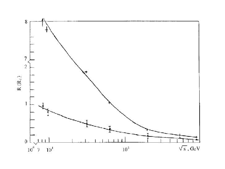
Figure 1:

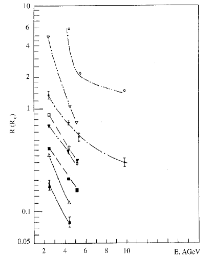
Figure 2:

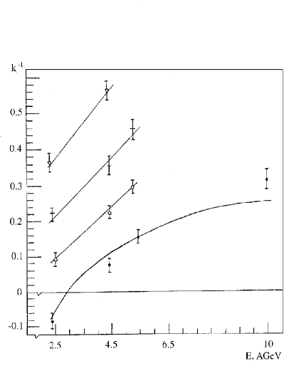
Figure 3:

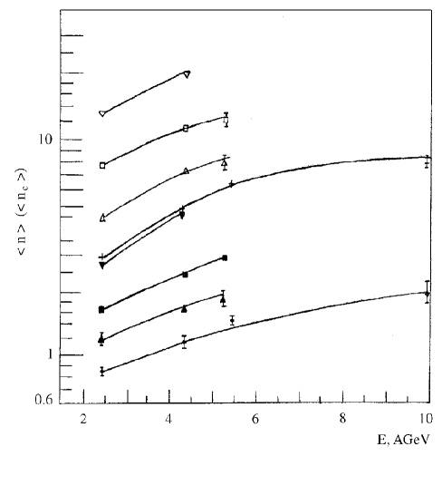
Figure 4:

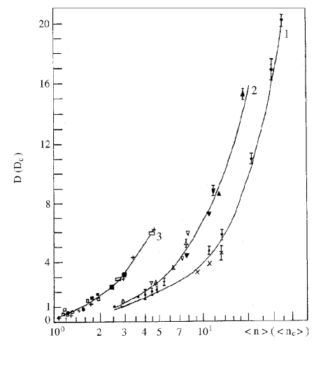
Figure 5:

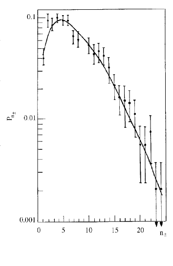
Figure 6: