Top Quark Physics: Future Measurements

Abstract

We discuss the study of the top quark at future experiments and machines. Top’s large mass makes it a unique probe of physics at the natural electroweak scale. We emphasize measurements of the top quark’s mass, width, and couplings, as well as searches for rare or nonstandard decays, and discuss the complementary roles played by hadron and lepton colliders.

1 Introduction

The recent observation of the top quark by the CDF and D0 collaborations[1, 2] has opened up the new field of top physics. The top quark’s measured mass of approximately 175 GeV[3] is nearly twice the mass of the next most massive particle, the $Z$ boson. It is also tantalizingly close to the natural electroweak scale, set by $v_{Higgs}=246$ GeV. While the Standard Model provides a theoretical context in which the top mass can be compared to (and found consistent with) other electroweak data, it offers no fundamental explanation for the top quark’s large mass, which arises from its large coupling to the symmetry-breaking sector of the theory. Precision measurements of the top mass, width, and couplings at future experiments may therefore lead to a deeper understanding of electroweak symmetry-breaking. Such measurements are possible in part because the top quark’s natural width of 1.4 GeV is much greater than the hadronization timescale set by $\Lambda_{QCD}$, so that top is completely described by perturbative QCD. Thus nature has presented us with the unique opportunity to study the weak interactions of a bare quark. It is the conclusion of this subgroup that precision studies of the top quark should be a high priority at future machines.

We have concentrated our attention on top physics at the following machines. The first is the so-called “TeV-33,” defined as a luminosity upgrade to the Fermilab Tevatron that would result in datasets of $\approx$30 fb^-1 at $\sqrt{s}=2.0$ TeV. For comparison, the goal for Tevatron Run II, scheduled to begin in 1999, is 2 fb^-1 at the same energy. We have also considered the top physics capabilities of the LHC, which will initially deliver 10 fb^-1/year and evolve to 100 fb^-1/year during high-luminosity running. Finally, we have considered an $e^{+}e^{-}$ linear collider operating at or above the $t\bar{t}$ threshold and delivering approximately 50 fb^-1/year. We have not explicitly considered a muon collider, although its top physics capabilities appear qualitatively similar to those of $e^{+}e^{-}$ machines provided that detector backgrounds can be controlled. We did not study a “super $pp$ collider” in the 60–200 TeV range. Other recent studies of top physics at the Tevatron can be found in the TeV2000 report[4] and references therein, while top physics at $e^{+}e^{-}$ machines has recently been reviewed by Murayama and Peskin[5] and Frey[6].

2 Top Quark Yields

At both hadron colliders and lepton colliders, most top quarks are produced in pairs. Each $t$ quark decays immediately to $Wb$, and the observed event topology depends on the decay mode of the two $W$’s. About 5% of $t\bar{t}$ decays are to the “dilepton” final state, which occurs when both $W$’s decay to $e\nu$ or $\mu\nu$. The “lepton+jets” final state occurs in the 30% of $t\bar{t}$ decays where one $W$ decays into $e\nu$ or $\mu\nu$ and the other decays into quarks. The remaining 65% of the decays are to final states containing $\tau$ leptons or hadronic jets. In this section we discuss the yields in these channels at future colliders.

2.1 Top Yields at Hadron Colliders

The dominant top quark production mechanism at hadron colliders is pair production through $q\bar{q}$ or $gg$ annihilation. The relative contribution of these two processes at the Tevatron is about 90%–10%, while at the LHC these percentages are reversed. The cross section for top pair production has been calculated by several authors[7]. For $p\bar{p}$ collisions at the planned Tevatron energy of $\sqrt{s}=2.0$ TeV, the cross section for $m_{t}=175$ GeV is calculated to be 7.5 pb, with an uncertainty estimated by various groups to be 10-30%. This is a 40% increase over the cross section at 1.8 TeV, and underscores the importance of even modest upgrades to the Tevatron energy. Thus a 30 fb^-1 Tevatron run would result in about 225,000 produced $t\bar{t}$ pairs. The LHC ($pp$ collisions at $\sqrt{s}=14$ TeV) is a veritable top factory, with a calculated $t\bar{t}$ production cross section of about 760 pb. This would result in about 7.6 million produced $t\bar{t}$ pairs per experiment in one year of low-luminosity LHC running.

In addition, single top quarks can be produced through electroweak processes such as $W$-gluon fusion or the production of an off-shell $W$ that decays to $t\bar{b}$[8]. The single-top production cross section is about 1/3 the $t\bar{t}$ cross section at both the Tevatron and the LHC. The single-top channels are of particular interest for measurements of the top quark width and $V_{tb}$ as described below.

Studies of the top quark at hadron colliders emphasize the dilepton and lepton+jets decay modes. Because these final states contain isolated high-$P_{T}$ lepton(s) and missing energy, they are relatively easy to trigger on and reconstruct. The dilepton mode has low backgrounds to begin with, while backgrounds in the lepton+jets channel can be reduced to an acceptable level by a combination of kinematic cuts and $b$-tagging. Recently CDF has demonstrated that top signals can be identified in the $\tau$ and all-hadronic decay modes as well, but to establish benchmark yields for future experiments it is useful to focus on the dilepton and lepton+jets final states. These yields are obtained from current CDF and D0 acceptances by including the effects of planned upgrades such as full geometrical coverage for secondary-vertex $b$-tagging and improved lepton-ID in the region $1<|\eta|<2.5$[4]. These acceptances are believed to be representative of any hadron collider detector with charged particle tracking in a magnetic field, good lepton identification, and secondary-vertexing capability. The assumptions include:

• High-$P_{T}$ charged lepton identifiction with good efficiency for $|\eta|<2$

• Secondary-vertex $b$-tagging with an efficiency of 50-60% per $b$-jet for $|\eta|<2$

• Ability to tag “soft leptons” from $b\rightarrow l\nu X$ with an efficiency of about 15% per $b$ jet

• Double $b$-tag efficiency of about 40% per $t\bar{t}$ event. Double-tagged events are a particularly clean sample with low combinatoric background and are well-suited for measurement of the top mass.

Table 1 shows the expected yields and signal/background at the Tevatron. The acceptance of the LHC detectors is expected to be comparable to that of the Tevatron experiments, so to first order the yields at the LHC will be greater by a factor equal to the ratio of the cross sections, approximately 100.

Table 1: Expected top yields at the Tevatron.

Mode	2 fb-1	30 fb-1	S/B
Dilepton	80	1200	$5:1$
$l+\geq 3$ jets / 1 $b$	1300	20,000	$3:1$
$l+\geq 4$ jets / 2 $b$	600	9000	$12:1$
Single top (all)	170	2500	1:2.2
Single top ($W^{*}$)	20	300	1:1.3

2.2 Top Yields at the NLC

The $t\bar{t}$ cross section due to $s$-channel $e^{+}e^{-}$ annihilation mediated by $\gamma,Z$ bosons increases abruptly at threshold, reaches a maximum roughly 50 GeV above threshold, then falls roughly as the point cross section ($\sigma_{pt}=87({\rm fb})/s({\rm TeV})$) at higher energy. At $\sqrt{s}=500$ GeV the lowest-order total cross section for unpolarized beams with $m_{t}=180$ GeV is $0.54$ pb. The electron beam will be highly polarized ($\sim 90\%$), and this has a significant effect on $t\bar{t}$ production. The lowest-order cross section becomes $0.74$ pb ($0.34$ pb) for a fully left-hand (right-hand) polarized electron beam. A design year of integrated luminosity (50 fb^-1) at $\sqrt{s}=500$ GeV corresponds to roughly $25\times 10^{3}$ $t\bar{t}$ events. The cross sections for $t$-channel processes, resulting, for example, in final states such as $e^{+}e^{-}t\bar{t}$ or $\nu\bar{\nu}t\bar{t}$, increase with energy, but are still relatively small. If it turns out that electroweak symmetry breaking is strongly coupled, this latter process then turns out to be of particular interest, as emphasized by Barklow[9].

The $t\bar{t}$ are produced polarized and, due to initial-state bremsstrahlung and gluon radiation, are not always back to back. According to expectations, the weak decay $t\rightarrow bW$ proceeds before hadronization can occur. This allows the possibility to perform, in principle, a complete reconstruction in an environment with little additional hadronic activity. The rapid top decay also ensures that its spin is transferred to the $bW$ system, which opens up unique opportunities to probe new physics, as will be explored in Section 7.

The emphasis of most simulations to date has been to perform a largely topological event selection, taking advantage of the multi-jet topology of the roughly $90\%$ of $t\bar{t}$ events with 4 or 6 jets in the final state. Therefore, cuts on thrust or number of jets drastically reduces the light fermion pair background. In addition, one can use the multi-jet mass constraints $M($jet-jet$)\approx M_{W}$ and $M($3-jet$)\approx m_{t}$ for the cases involving $t\rightarrow bqq^{\prime}$. Simulation studies[10] have shown that multi-jet resolutions of 5 GeV and 15 GeV for the 2-jet and 3-jet masses, respectively, are adequate and readily achievable with standard detector resolutions. A detection efficiency of about 70% with a signal to background ratio of 10 was attained in selecting 6-jet final states just above threshold. These numbers are typical also for studies which select the 4-jet$+\ell\nu$ decay mode.

Another important technique is that of precision vertex detection. The present experience with SLC/SLD can be used as a rather good model of what is possible at NLC. The small and stable interaction point, along with the small beam sizes and bunch timing, make the NLC ideal for pushing the techniques of vertex detection. At this meeting, Jackson presented[11] simulation results indicating that $b$-jets can be identified with an efficiency of 60% with about 97% purity. This has important implications for top physics. Rather loose $b$-tagging, applied in conjunction with the standard topological and mass cuts mentioned above, imply excellent prospects for an efficient and pure top event selection. Detailed studies employing such a combination of techniques have not yet been performed, however, and it will be interesting to see what can be achieved.

The background due to $W$-pair production is the most difficult to eliminate. However, in the limit that the electron beam is fully right-hand polarized, the $W^{+}W^{-}$ cross section is dramatically reduced. This allows for experimental control and measurement of the background. On the other hand, the signal is also reduced, albeit to a much smaller degree, by running with right-polarized beam. A possible strategy might be to run with right-hand polarized beam only long enough to make a significant check of the component of background due to $W$ pairs.

3 Mass Measurement at Hadron Colliders

The precision with which the top quark mass, $m_{t}$, can be measured is an interesting and important benchmark of proposed future experiments. Within the Standard Model and its extensions $m_{t}$ is a fundamental parameter whose value is related to the Higgs sector of the electroweak interaction[12]. As such, it is desirable to have a measurement with a precision comparable to that of other electroweak parameters, typically of the order of $<1\%$. This would correspond to an uncertainty of about 2 GeV in $m_{t}$. Extensions to the Standard Model often predict the value of $m_{t}$, and a sufficiently precise measurement of $m_{t}$ could also help distinguish between different models. For this purpose, it would be of interest to measure the top quark mass with a precision of about 1 GeV[13].

The measurements provided by contemporary experiments at CDF and at D0[14, 15] have been studied in sufficient detail that the expected precision at hadron colliders can be conservatively extrapolated with some confidence[4, 16, 17]. Issues relevant to this extrapolation are presented below as understood from studies of the TeV2000 work but are believed to be a fair representation of the challenges for experiments at the LHC as well. Other mass-measurement techniques also exist but have not been explored at the same level of detail. Control of systematic uncertainties is likely to be the critical issue in the measurement of $m_{t}$ in any method.

3.1 Constrained Fits in Lepton+jets Decays

The most precise direct determination of the top mass currently comes from reconstructing candidate top events with a $l\nu{\rm+\ jets}$ topology. Assuming that the momenta of all final-state partons except the one neutrino are measured, that the transverse energy of the system is conserved, that the $t$ and $\bar{t}$ quarks have a common mass, and that there are two real $W$ bosons results in an overconstrained system from which the event kinematics can be obtained. The method is of additional interest because it provides a means of determining other kinematic features of the $t\bar{t}$ decay such as their transverse momentum or total invariant mass.

The accuracy with which the technique can reconstruct the kinematics is limited by the ambiguity in making the correspondence between observed jets and underlying quarks. Without relying on $b$-tagging, there are 12 different ways to label the jets as either a $b$-quark or a light quark from a $W$ and to associate them with either the $t$ or $\bar{t}$ quark. If one jet is $b$-tagged, there are six such combinations and if two jets are tagged then there are two possibilities. Additionally, by requiring the $\nu-{\rm lepton}$ invariant mass to equal $M_{W}$, the component of the $\nu$ momentum along the direction of the beam axis can be determined up to a quadratic ambiguity. Thus, there are twice as many kinematically consistent solutions for each event. By selecting the single solution which best fits the $t\bar{t}$ hypothesis according to a $\chi^{2}$ test, the reconstruction of the kinematics results in an estimated top mass for each event. The measured top mass is obtained by comparing the event mass distribution to that predicted by Monte Carlo models for different top masses using a maximum likelihood method.

Two sources of uncertainty limit the precision with which this technique can be used to measure $m_{t}$. The first is the statistical uncertainty which arises from the finite detector resolution and the limited number of events. Monte Carlo studies indicate that this source of uncertainty decreases like $\sigma/\sqrt{N}$. The intrinsic resolution, $\sigma$ is itself composed of two pieces. The first piece is the resolution for those events where the correct assignment is made between the partons and jets and the second piece is the resolution for the cases where the incorrect parton-jet assignment is made. The relative contribution of each of these sources varies according to the tagging information available. Using no tagging information results in a resolution dominated by the misassigned component but also results in the largest number of top events. Requiring two tagged jets results in the smallest resolution because of the much higher fraction of events with correctly assigned jets but has a corresponding loss of efficiency. Table 2 summarizes the tradeoff in the tagging requirements with the expected statistical uncertainty for a luminosity of 2 fb^-1 at the Tevatron or LHC. As shown, the ultimate statistical uncertainty is a fraction of a GeV for any of the three samples.

Table 2: Expected statistical precision for measurement of top quark mass for differently $b$-tagged subsamples.

Tags	Number of $t\bar{t}$ Events	Background	$\sigma_{m_{t}}$ (GeV)
0	20000	40000	0.3
1	12000	3000	0.3
2	4000	100	0.3

The second source of uncertainty in the top mass measurement is systematic. The largest sources of systematic uncertainty arise from differences between the observed mass distribution and the prediction from Monte Carlo and detector simulations. Such differences arise, for instance, in the jet-parton $E_{T}$ scale and in the modeling of $t\bar{t}$ production and decay. Table 3 shows the expected systematic uncertainties for the constrained fit technique at future hadron colliders with an integrated luminosity of ${\rm 2\ fb^{-1}}$.

Table 3: Expected systematic uncertainties in the measurement of $m_{t}$ for an integrated luminosity of 10 fb-1 at a hadron collider.

Systematic	$\sigma_{m_{t}}$ (GeV)
Jet-Parton $E_{T}$ Scale	2.0
Event Modeling	2.0
Background Shape	0.3

Based on present understanding of $t\bar{t}$ event reconstruction, systematic uncertainties are expected to limit the ultimate precision with which the top mass can be measured. The most important of these are the precision with which the jet $E_{T}$ scale can be determined and understanding the multijet environment of $t\bar{t}$ production.

3.2 Jet $E_{T}$ Scale

Jets are typically identified using fixed-cone clustering algorithms. Monte Carlo models are used to derive a correspondence between observed jet energies and the momenta of the underlying partons. An understanding of the $E_{T}$ scale therefore involves both theoretical uncertainties in the model of parton fragmentation to a jet, and experimental uncertainties in the detector’s measurement of the jet energy.

Figure 1 shows a comparison of energy flow in an annulus about single jets produced in association with $W$ decays. Comparison of jet anatomies with this technique between data and Monte Carlo can be used to quantify theoretical uncertainties in the jet-parton $E_{T}$ scale. Such studies will likely improve with the size of the control samples and indicate that theoretical uncertainties in the jet-parton $E_{T}$ scale can be managed to better than 1 GeV in future experiments.

Figure 1: Energy flow in annular region around single jets produced in association with $W$ bosons.

It is more difficult to reduce the detector effects below the present typical value of 3-4 GeV, and this source of uncertainty could limit the ultimate precision of the top mass measurement. New possibilities for understanding the jet-parton $E_{T}$ scale are offered by control samples that will be available in future high-statistics data sets. One example is to use the $W\rightarrow q\bar{q}^{\prime}$ decay in the top-quark events themselves to calibrate the scale. The dijet mass distribution for $W\rightarrow q\bar{q}^{\prime}$ candidates in top events can be compared to a model where the jet $E_{T}$ scale is varied and used to fit the scale. A toy Monte Carlo can be used to simulate many such experiments with the appropriate combinations of signal and background. Relying on the CDF detector as a model, Fig. 2 shows the distribution of extracted Jet $E_{T}$ scale using the technique on experiments of varying signal-background composition. Each entry in the histogram is the extracted $E_{T}$ scale obtained by the method for a single toy experiment where the true ${\rm E}_{\scriptscriptstyle\rm T}$ scale was perfect. The width of the distribution is the expected precision with which the Jet $E_{T}$ scale can be estimated and is seen to be typically of order 1%, or a factor of 3-4 better than currently derived from sample of about $100{\rm pb^{-1}}$. We therefore conclude that the jet-parton $E_{T}$ scale can be controlled to the $\sim$1% level, implying a corresponding uncertainty in the top quark mass of about the same size.

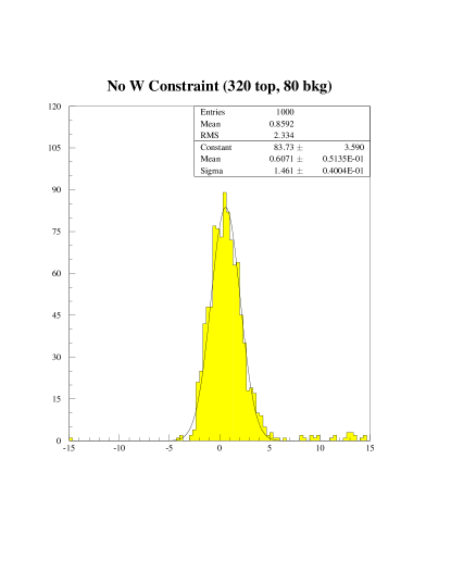
Figure 2: Estimated jet-parton $E_{T}$ scale extracted from toy Monte Carlo experiments. Each entry is the measured jet-parton $E_{T}$ scale obtained from the reconstructed $W\rightarrow q\bar{q}^{\prime}$ decay in top events. Simulated experiments consisted of samples of top and background typical for Tevatron Run II data samples.

3.3 Uncertainties in Kinematic Modeling

In addition to the jet-parton $E_{T}$ scale, uncertainties in the top quark mass can arise from the uncertainty in modeling the jet environment of top decays. Constrained fitting techniques typically associate the leading four jets with the two $b$ jets and two jets from hadronic $W$ decay; however, initial- or final-state gluon emission may contaminate the leading four jets with jets that do not arise directly from $t\bar{t}$ decay, resulting in a more confused event kinematics. This effect is modelled by parton shower Monte Carlo programs, such as Herwig. Figure 3 shows the invariant mass distribution for top events for those events where extra gluon radiation results in a leading jet not associated with the partons directly from the $t\bar{t}$ decay. Conservatively assuming no information is available on the rate of such events implies a corresponding uncertainty on the top quark mass of 3 GeV. This uncertainty is currently limited by the lack of a large sample of top quarks with which the modeling of jet kinematics can be tested. At the same time, significant theoretical and phenomenological work has proceeded towards an understanding of gluon radiation in $t\bar{t}$ events[19]. In datasets with large number of top events, it is evident that the understanding of this and other related theoretical issues will improve and indeed will be a source of interesting physics as well.

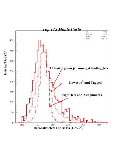
Figure 3: Reconstructed mass spectra from $t\bar{t}$ Monte Carlo ($m_{t}=175$ GeV) with and without the presence of hard gluon radiation.

3.4 Other Mass Measurement Techniques

While the constrained fit technique provides the most precise determination available, other techniques exist, although they have not been explored in the same depth. As described above, the measurement of the top quark mass can be viewed as simply comparing a kinematic feature (such as the reconstructed mass) with that predicted by models for different top masses. The same philosophy can be applied, for instance, to underconstrained topologies such as events where the $t\bar{t}$ decay in the dilepton mode[18]. This technique is statistically less powerful than the lepton + jets method and suffers from similar systematics due to the jet energy scale; however the method may complement the more conventional analysis. Another intriguing possibility is to measure the decay length of $B$ mesons associated with the $b$-jets in top decays. The decay length is correlated with the $b$-jet boost and hence the mass. It has the additional attractive feature of being a mostly tracking-based measurement, and is therefore much less dependent on the jet-parton $E_{T}$ scale. The systematics in this technique, which include uncertainty in the top quark transverse momentum distribution, need further study.

3.5 Outlook

It appears that with available technology, the top quark mass can be measured to a precision of about 1%, with the caveat that the understanding of theoretical issues dealing with the jet environment in top decays is thought to be limited primarily by the small number of events presently available. It is hoped that systematic effects from these sources can be brought under control with larger samples of data. While it is not clear that detector resolution can be substantially improved, it appears that a program that relies on control samples in the data can manage the leading systematic uncertainties to the 1% level. The ultimate resolution as represented by the statistical uncertainty will be on the order of a few hundred MeV. The issues of the modeling of the top kinematics will be crucial but at the same time will be very interesting tests in and of themselves. In short, our present understanding of $t\bar{t}$ reconstruction at hadron colliders supports the expectation that the measurement of $m_{t}$ at either the LHC or at an upgraded Tevatron can be made with the precision thought to be needed to provide insights into the Electroweak and Higgs sector of the Standard Model.

4 Measurements at the $t\bar{t}$ Threshold

Production of $t\bar{t}$ near threshold in $e^{+}e^{-}$ (or $\mu^{+}\mu^{-}$) annihilation offers qualitatively unique opportunities for top physics studies. In addition, in many cases, it promises to allow the most precise measurements of key parameters. The cross section in the $t\bar{t}$ threshold region depends sensitively on $m_{t}$, $\alpha_{s}$, and $\Gamma_{t}$, and interestingly, also depends on the top-Higgs Yukawa coupling, $\lambda_{t}$, and $m_{H}$. In this section we briefly discuss the phenomenology and prospects for these measurements near threshold. The $\mu^{+}\mu^{-}$ case is not expected to differ significantly from $e^{+}e^{-}$ except for radiative and accelerator effects, and is not otherwise specifically discussed.

4.1 Threshold Shape

In Fig. 4 we show the cross section for $t\bar{t}$ production as a function of nominal center-of-mass energy $E_{\rm cm}=\sqrt{s}$ for $m_{t}=175$ GeV. The theoretical cross section, indicated as curve (a), is based on the results of Strassler and Peskin[20] with $\alpha_{s}(M_{Z}^{2})=0.120$, infinite Higgs mass, and nominal Standard Model couplings. The characterization of the top threshold is an interesting theoretical issue, and the theoretical cross section and its associated phenomenology have been extensively studied[21, 20, 22, 23, 24, 10]. The energy redistribution mechanisms of initial-state radiation, beamstrahlung, and single-beam energy spread, have been successively applied to the theoretical curve of Fig. 4. Hence, curve (d) includes all effects. We begin the discussion of top threshold physics with a brief overview of these radiative and accelerator effects, which are especially important at $t\bar{t}$ threshold because of the relatively sharp features in the cross section.

Figure 4: Production cross section for top-quark pairs near threshold for $m_{t}=175$ GeV. The theoretical cross section is given by curve (a). The following energy redistribution effects have been applied to the theory for the remaining curves: (b) initial-state radiation (ISR); (c): ISR and beamstrahlung; (d): ISR, beamstrahlung, and single-beam energy spread.

The effects of initial-state radiation (ISR) are appreciable for high energy electron colliders, where the effective perturbative expansion parameter for real photon emission, rather than $\alpha/\pi$, is $\beta={2\alpha\over\pi}(\ln(s/m_{e}^{2})-1)\approx 1/8$ for $\sqrt{s}=500$ GeV. We use a standard calculation[25] of ISR, which sums the real soft-photon emission to all orders and calculates the initial state virtual corrections to second order. An analytic calculation[26] provides a good approximation for the effects of beamstrahlung at the NLC. The figure of merit in the calculation is $\Upsilon=\gamma(B/B_{c})$, where $\gamma=E_{\rm beam}/m_{e}c^{2}$, $B$ is the effective magnetic field strength of the beam, and $B_{c}=m_{e}^{2}c^{3}/e\hbar\approx 4\times 10^{9}$ T. When $\Upsilon\ll 1$ the beamstrahlung is in the classical regime and is readily calculated analytically. For example, in the case of the SLAC X-band NLC design, we have $B\approx 6\times 10^{2}$ T and $\Upsilon\approx 0.08$ at $\sqrt{s}=500$ GeV. In this case, there is an appreciable probability for a beam electron (or positron) to emit no photons. So the spectrum is well-approximated as a delta function at $E=E_{\rm cm}$ with a bremsstrahlung-like tail extending to lower energies. The fraction of luminosity within the “delta function piece” of the spectrum resolves the $t\bar{t}$ threshold structure, while the remaining luminosity is, for the most part, shifted in energy well away from threshold. Hence, the primary effect of beamstrahlung is to reduce the useful luminosity at threshold. The delta-function fraction of luminosity for the nominal SLAC X-band NLC design at 500 GeV, for example, is $43\%$. The energy loss spectrum for initial-state radiation, like beamstrahlung, has a long tail, and is also qualitatively similar to beamstrahlung in that it is rather likely to have negligibly small energy loss. For example, $\approx 50\%$ of the total luminosity results in a center of mass collision energy within $0.1\%$ of the nominal $\sqrt{s}\>$[27].

Hence, to good approximation the combined effect of these processes is an effective reduction of luminosity at the nominal $\sqrt{s}$ due to beam particles which have undergone energy loss $>\Gamma_{t}$. We see this in Fig. 4, although there is clearly also some smearing out of the threshold shape due to small energy loss. Of course, there is no control of ISR, except for the choice of beam energy and accelerated particle—here a muon collider would benefit from the decreased radiation, where the expansion parameter $\beta$ decreases from $0.12$ to $0.07$. On the other hand, the accelerator design will have some effect on the resulting beamstrahlung spectrum. For example, in changing $\sqrt{s}$ from 500 GeV to $t\bar{t}$ threshold, one might choose to keep the collision point angular divergences constant, in which case the spot sizes would increase roughly as $500/350$, resulting in lower luminosity and decreased beamstrahlung. Alternatively, scaling the energy at constant beta would result in decreases only by $\sim\sqrt{500/350}$. So one can expect for the SLAC design to have the fraction of luminosity unaffected by beamstrahlung (the delta-function fraction) to be $\sim 50\%$ at $t\bar{t}$ threshold.

An additional accelerator effect on the threshold shape results from the energy spread of each beam in its respective linac. This is the additional effect included in curve (d) of Fig. 4, and is characterized by the FWHM of the energy spread for a single beam, $\Delta E/E$, which is a symmetric, non-centrally peaked distribution about the nominal beam energy. The calculation of Fig. 4 used $\Delta E/E=0.6\%$. This quantity can be adjusted during operation, typically by $\pm 50\%$, within some bounds set by the accelerator design. In Section 4.5 we discuss the measurement of the luminosity spectrum resulting from these effects.

4.2 Sensitivity to $m_{t}$ and $\alpha_{s}$

The threshold enhancement given by the predicted cross section curve (a) of Fig. 4 reflects the Coulomb-like attraction of the produced top pair due to the short-distance QCD potential

$$V_{\rm QCD}\sim-C_{F}{\alpha_{s}(\mu)\over r}\ ,$$ (1)

where $C_{F}=4/3$ and $\mu$ is evaluated roughly at the scale of the Bohr radius of this $t$-$\bar{t}$ bound system: $\mu\sim\alpha_{s}m_{t}$. This bound state exists, on average, for approximately one classical revolution before one of the top quarks undergoes weak decay. The level spacings of the QCD potential, approximately given by the Rydberg energy, $\sim\alpha_{s}^{2}m_{t}$, turn out to be comparable to the widths of the resonance states, which are $\approx 2\Gamma_{t}$. Therefore the various bound states become smeared together, where only the bump at the position of the 1S resonance (at about $347.5$ GeV in Fig. 4) is distinguishable. The infrared cutoff imposed by the large top width also implies[21] that the physics is independent of the long-distance behavior of the QCD potential. The assumed intermediate-distance potential is also found[10] to have a negligible impact. Hence, the threshold physics measurements depend on the short-distance potential (Eq. 1) of perturbative QCD.

An increase of $\alpha_{s}$ deepens the QCD potential, thereby increasing the wave function at the origin and producing an enhanced 1S resonance bump. In addition, the binding energy of the state varies roughly as the Rydberg energy $\sim\alpha_{s}^{2}m_{t}$. So the larger $\alpha_{s}$ has the combined effect of increasing the cross section as well as shifting the curve to lower energy. The latter effect would also occur, of course, for a smaller $m_{t}$. Therefore, measurements of $\alpha_{s}$ and $m_{t}$ extracted solely from a fit to the threshold cross section will be partially correlated, but separable.

In addition to the measurement of the threshold excitation curve, an interesting and potentially quite useful measurement near threshold is based upon the observation that the lifetime of the bound state is determined by the first top quark to undergo weak decay, rather than by annihilation. This implies that the reconstructed kinetic energy (or momentum) of the top decay products reflect the potential energy of the QCD interaction before decay. Hence, a measurement of the momentum distribution will be sensitive to $V_{\rm QCD}$ and $\alpha_{s}$. A larger $\alpha_{s}$ produces a deeper $V_{\rm QCD}$, hence increasing the kinetic energy given to the top decay products when the “spring” breaks upon decay of the first of either $t$ or $\bar{t}$. The theory[22, 24] and phenomenology[10, 28] of this physics have been extensively studied. The observable used to characterize the distribution is the peak of the momentum distribution, $p_{0}$, which shifts to larger values for larger $\alpha_{s}$. The best $\sqrt{s}$ to run the accelerator for this measurement is about 2 GeV above the 1S peak. The studies show that $p_{0}$ is indeed sensitive to $\alpha_{s}$. The measurement also has useful sensitivity to the top width, which arises because a variation in $\Gamma_{t}$ moves the average $t$–$\bar{t}$ separation $r_{d}$ at the time of decay, and hence the average potential energy $V_{\rm QCD}(r_{d})$.

A number of studies have been carried out to simulate measurements at $t\bar{t}$ threshold. Typically one fixes the width and fits the threshold shape for the correlated quantities $m_{t}$ and $\alpha_{s}(M_{Z}^{2})$. For example, a simulation[10] assuming $m_{t}=150$ GeV used 1 fb^-1 for each of 11 scan points. If $m_{t}$ and $\alpha_{s}(M_{Z}^{2})$ are left as free parameters, then a simultaneous 2-parameter fit results in errors of $200$ MeV and $0.005$, respectively. If one performs a single-parameter fit, holding the other quantity to a fixed value, the resulting sensitivities approach $100$ MeV and $0.0025$. An update[29] of the 2-parameter fit for $m_{t}=170$ GeV gives errors of 350 MeV and $0.007$ for the same 11-point scan. A similar simulated scan[30] assuming $m_{t}=180$ GeV and 5 fb^-1 for each of 10 scan points resulted in single-parameter errors of $120$ MeV and $0.0025$ for $m_{t}$ and $\alpha_{s}$, respectively. We see that while the error on $m_{t}$ is remarkably good, the error on $\alpha_{s}(M_{Z}^{2})$ is less impressive relative to current measurements. Of course, it will be very interesting at the outset to compare the threshold excitation curve with expectations to see, for example, that the $\Delta R$ increase is consistent with the charge and spin of the top quark. But if the threshold curve can indeed be fit by QCD, then a reasonable strategy for extracting $m_{t}$ might be to fix $\alpha_{s}(M_{Z}^{2})$ at the World average value and perform the single-parameter fit of the threshold to extract $m_{t}$. The studies cited above have also examined the use of the top momentum ($p_{0}$) technique. It improves somewhat the precision of the fitted parameters, typically improving both the $m_{t}$ and $\alpha_{s}(M_{Z}^{2})$ errors by $\sim 20\%$. The $p_{0}$ measurement also has different correlation between mass and strong coupling than the cross section, hence providing a useful crosscheck. In fact, Fujii, et al. have emphasized that if the scan energy is referenced to the measured position of the 1S peak, rather than with respect to $2m_{t}$ or $\sqrt{s}$, then the $p_{0}$ measurement becomes independent of $m_{t}$. Carried out in this way, the top momentum measurement would indeed be invaluable as a crosscheck. Systematic errors associated with the threshold measurements and scan strategies are discussed briefly in Section 4.5.

4.3 The Top Yukawa Potential

In addition to the QCD potential, the Standard Model predicts that the $t\bar{t}$ pair is also subject to the Yukawa potential associated with Higgs exchange:

$$V_{Y}=-{{\lambda_{t}^{2}}\over{4\pi}}{{e^{-m_{H}r}}\over{r}}\ ,$$ (2)

where $m_{H}$ is the Higgs mass and $\lambda_{t}$ is the Yukawa coupling,

$$\lambda_{t}=\bigl{[}\sqrt{2}G_{F}\bigr{]}^{1/2}\,\beta_{H}m_{t}=\beta_{H}m_{t}/v_{\rm Higgs}$$ (3)

The dimensionless parameter $\beta_{H}$ is discussed below. Because of the extremely short range of the Yukawa potential, its effect is only on the wave function at the origin, and hence provides a shift of the cross section across the threshold region with a slight energy dependence. Fig. 5 gives a calculation[31] of this effect. It is quite interesting that because of the large top mass, the Yukawa potential may indeed be observable in this system. From the various $m_{H}$ curves given in this calculation, we clearly see the exponential cutoff of the Yukawa potential for large $m_{H}$.

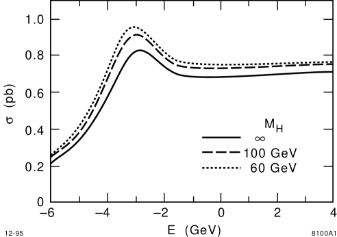
Figure 5: Cross section near threshold for different Higgs masses due to the Yukawa potential. $m_{t}=180$ GeV/c² was assumed. The abscissa center-of-mass energy is relative to $2m_{t}$.

It is assumed here, of course, that the Higgs bosons(s) will have already been discovered when such a measurement is undertaken. However, the Yukawa coupling to fermions is a fundamental element of electroweak theory, and very likely can only be tested with top quarks. The factor $\beta_{H}$ in Eq. 3 is used to parameterize the strength of the Yukawa coupling and possible deviations from the Standard Model, in which $\beta_{H}=1$. For example, in two-Higgs-doublet models $\beta_{H}$ is complex with real (imaginary) part proportional to $1/\sin\beta$ ($1/\tan\beta$), where $\tan\beta$ is the usual ratio of Higgs vacuum expectation values. Hence, these measurements can also be used to help distinguish between different models of the Higgs sector. In Section 8  we review the prospects for the measurement of $\lambda_{t}$ in open top production. However, the effect of the Higgs field on the $t\bar{t}$ state at threshold is unique and it is interesting to see how sensitive a threshold scan might be. Figure 6  shows a calculation of the cross section across threshold for different values of $\beta_{H}$. The values $m_{t}=175$ GeV and $m_{H}=300$ GeV were used and all radiative and accelerator effects are included. (Hence, the $\beta_{H}=1$ curve corresponds to curve (d) of Fig. 4.) So one would have a reasonable sensitivity to this physics with some dedicated running just above threshold. Fujii[29] also applied the previously mentioned 11 point scan of 1 fb^-1 per point to the measurement of $\beta_{H}$. For larger $m_{t}$ the accuracy improves, as expected, and at $m_{t}=170$ GeV he finds that $\beta_{H}$ can be measured to $25\%$.

Figure 6: Threshold shape for various (real) values of the Yukawa coupling strength $\beta_{H}$. All radiative and beam effects are included, and $m_{t}=175$ GeV, $m_{H}=300$ GeV are used. The different curves corresond to $\beta_{H}=1.5$, $1.0$, and $0.5$, as indicated.

4.4 The Top Width

Running at $t\bar{t}$ threshold allows a direct measurement of the top quark width, $\Gamma_{t}$, without making any assumptions about top decay modes. As discussed below in Section 5, this is especially important for non-standard decays in which top does not decay to $W$. On general grounds, we expect the peak cross section of a 1S quarkonium bound state to vary with the total width as $\Gamma_{t}^{-1}$, independent of decay modes. This is shown by the theoretical curves given in the upper plot of Fig. 7. After applying ISR and beam effects, the width is affected as shown in the lower plot of Fig. 7. In this case, we see that the cross section just below the 1S threshold is also quite sensitive to the width. The studies cited above indicate sensitivity to $\Gamma_{t}$ at the level of 10% for 50 fb^-1 of data. However, as discussed in the next section, any estimate will depend crucially on the scan strategy employed.

Figure 7: Threshold shape for various values of $\Gamma_{t}$. The upper plot is the theoretical prediction, while the lower plot includes all radiative and beam effects. The different curves corresond to $\Gamma_{t}/\Gamma_{t}^{\rm SM}=$ (a) $0.5$, (b) $0.8$, (c) $1.0$, (d) $1.2$, and (e) $1.5$. We assumed $m_{t}=175$ GeV, where the Standard Model width is $\Gamma_{t}^{\rm SM}=1.42$ GeV.

Yet another, quite different observable which is particularly sensitive to $\Gamma_{t}$ has been studied[32, 10] to help further pin down the physics parameters at threshold. The idea is summarized as follows. The vector coupling present with $Z$-$t$-$\bar{t}$ and $\gamma$-$t$-$\bar{t}$ can proceed to S and D-wave bound states. On the other hand, the axial-vector coupling present with $Z$-$t$-$\bar{t}$ gives rise to P-wave states. Hence, it is possible to produce interference between S and P-waves which gives rise to a forward-backward asymmetry ($A_{FB}$) proportional to $(v/c)\cos\theta$, where $\theta$ is the usual production polar angle in the $t\bar{t}$ rest system. Because of the large width of these states, due to the large $\Gamma_{t}$, they do overlap to a significant extent, and a sizeable $A_{FB}$ develops. The value of $A_{FB}$ varies from about 5% to 12% across the threshold, with the minimum value near the 1S resonance. Since the top width controls the amount of S-P overlap, we expect the forward-backward asymmetry to be a sensitive method for measuring $\Gamma_{t}$. In fact, this has been studied, again by the same groups as above. Although considerably less sensitive to $\Gamma_{t}$ than the threshold cross section (about a factor ten in terms of luminosity), this technique again provides a useful crosscheck of the threshold physics.

4.5 Systematic Effects and Scan Strategies

As indicated in Section 2.2, an efficient and pure event selection with good experimental controls appears to be possible. So we expect the outstanding systematic issue to be the characterization of the redistribution of collision energy due to radiation and beam effects, as discussed in Section 4.1. This can be quantified by a differential luminosity spectrum $d{\cal L}/dE$ which describes how the nominal center-of-mass energy $\sqrt{s}$ is distributed to $e^{+}e^{-}$ collision energies $E$. Of course, this must be determined in order to unfold the physics parameters from the experiemental scan points. One would hope to measure the luminosity expended at each scan point to $\sim 1\%$. Fortunately, it is not necessary to know the radiative and accelerator effects a priori at this level of precision. One can, in fact, make an independent measurement of the luminosity spectrum. As proposed by Frary and Miller[33], the idea is to measure the acollinearity distribution of final state particles in a $2\rightarrow 2$ process. Bhabha scattering turns out to be ideal. At intermediate scattering angles (about $\theta=20^{\circ}$ to $\theta=40^{\circ}$), Bhabha scattering has a rate $\sim 100$ times that of top production, the acollinearity can be measured with the requisite accuracy ($<1$ mrad), and it is theoretically well known at the 1% level. The acollinearity angle $\theta_{A}$ for a final-state $e^{+}e^{-}$ pair produced at scattering angle $\theta$ is related to the energy difference $\delta E$ of the initial-state $e^{+}e^{-}$ by $\delta E/E=\theta_{A}/\sin\theta$, where $E\approx E_{\rm beam}$ is their average energy. So starting with the theoretical distribution in $\theta_{A}$, one applies contributions due to ISR and beamstrahlung (and single-beam energy spread), whose functional forms are known, until the resulting distribution agrees with the measured one. One then applies this luminosity spectrum to the top scan data taken over the same running period.

The other related issue is the determination of the absolute energy scale, that is, the energy of the beams. This is presently done at the SLC using a spectrometer for each spent beam. The accuracy for $\sqrt{s}$ is 25 MeV ($0.03\%$). Scaling this same error to top threshold gives 100 MeV accuracy, which is at or below the level of error quoted above for a high statistics measurement of $m_{t}$. To measure the beam energy, the beams will be briefly taken out of collision, which eliminates beamstrahlung. (The beamstrahlung-reduced beam energy measured by the spectrometer is not equivalent to that seen by collisions since the two sample the beam populations differently.)

Most of the sensitivity to the threshold physics measurements of $m_{t}$, $\alpha_{s}$, $\Gamma_{t}$, and $\beta_{H}$ comes from the cross section scan across threshold, although as we have seen, the measurements of top momentum and the forward-backward asymmetry also provide useful input. These latter two techniques also are more difficult and demand more study to determine limiting systematics. Therefore, it is useful to consider how to extract the measurements solely from the cross section scan. From the discussions above we have seen that each physics quantity has a different effect on the threshold shape. So the physics goals will certainly define the scan strategy.

Expending even a modest fraction of a standard year of luminosity (50 fb^-1) at threshold would check the overall physics of the threshold system and would give an excellent measurement of the top mass at the level of $\sim 200$ MeV. To concentrate on the mass measurement, one would choose to expend luminosity where the cross section changes most rapidly, at about 346 to 347 GeV for $m_{t}=175$ GeV. Assuming a standard model width and fixing $\alpha_{s}$ from external measurements, in only $\sim 10$ fb^-1 one would reach the level of 100 MeV error, which is where the systematics of the absolute energy scale would be expected to become important.

Of course, one would really like to directly measure $\Gamma_{t}$ given this opportunity. From Fig. 7 we see that measuring the slope of the threshold rise is required to measure the width. So one would want to expend luminosity at about 344 and 348 GeV, as well. Fujii[29] finds that fixing $\alpha_{s}$ and performing a 2-parameter fit to $m_{t}$ and $\Gamma_{t}$, the usual $11\times 1$ fb^-1 scan gives (statistical) errors of 100 MeV for $m_{t}$ and $\delta\Gamma_{t}/\Gamma_{t}=16\%$. If $\Gamma_{t}$ looked interesting one could go after the especially sensitive scan energies. Apparently, the error could be pushed by statistical scaling until the luminosity systematics become important, at the level of $\sim 1\%$. Hence, a scan chosen in this way would push the measurement of $\Gamma_{t}$ to about 5% in 50 fb^-1.

Observing the effect of the Yukawa potential would be unique, and checking the Yukawa coupling would be a fundamental test. First of all, one would want to check that the cross section at the 1S (about $347.5$ GeV for $m_{t}=175$ GeV) is as expected given the value of $m_{H}$ taken from other measurements (see Fig. 5). This would establish whether the strength of the Yukawa potential is as expected. Then, from Fig. 6 we see that one or two scan points above the 1S would establish the slope and provide a measurement of $\beta_{H}$. Again, if the physics demands it, this measurement could be pushed statistically, eventually to the level of $\sim 1\%$.

In all cases, a reasonable fraction of the luminosity will have to be expended just below threshold to measure the background. This fraction would depend, of course, on the ultimate purity of the event selection, but 10 to 20% is a reasonable guess. Since $W^{+}W^{-}$ production is expected to be the largest background, an important experimental control is provided by the electron-beam polarization. Flipping between left and right-handed polarizations would give a huge change in this background (since the cross section for right-handed production is tiny) by a predictable amount. So one should expect that the background fraction can be accurately determined.

In summary, the physics quantities of interest at threshold each have different effects on the shape of the threshold curve, and can be optimally extracted with a cross section scan employing carefully chosen scan points. In addition, measurements of the top momentum and forward-backward asymmetry at threshold provide useful crosschecks of the same quantities. A modest data set of 10 fb^-1 would provide a check of the overall phenomenology and would allow a measurement of $m_{t}$ with an error of 100 MeV to 350 MeV, depending upon the scan and whether $\alpha_{s}$ is fixed or allowed to be a free parameter. This luminosity would allow initial measurements of $\alpha_{s}(M_{Z}^{2})$, $\Gamma_{t}$, and the Yukawa coupling $\beta_{H}$ with errors at the level of $0.005$, 16%, and 25%, respectively. Physics priorities would push optimization of the scan strategy to concentrate on a subset of these quantities, so that with 50 fb^-1 one could attain errors of 100 MeV ($m_{t}$), 0.0025 ($\alpha_{s}(M_{Z}^{2})$), 5% ($\Gamma_{t}$), or 10% ($\beta_{H}$). At the current level of understanding, the measurements become systematics limited near these errors for $m_{t}$ and $\alpha_{s}$, but the width and Yukawa coupling measurements could be pushed to the level of $\sim 1\%$.

5 The Top Quark Width and $V_{tb}$ at Hadron Colliders

In the Standard Model, the top quark decays essentially 100% of the time to $Wb$, and the rate for this process leads to a firm prediction for the top width of $\Gamma_{t}=1.4$ GeV (for $m_{t}=175$ GeV), corresponding to a lifetime of $<10^{-25}$s. A measurement of $\Gamma_{t}$ is of great interest because $\Gamma_{t}$ is affected by any nonstandard decay modes of the top, whether visible or invisible. Future experiments must therefore address the related questions “Does top always decay to $Wb$?” and “Is $V_{tb}$ equal to 1?”. That these questions are not equivalent can be seen by considering the situation with $b$ decays, in which the $b$ quark decays essentially 100% of the time to $Wc$ despite the fact that $V_{cb}\approx 0.04$. The relatively narrow width of the $b$ is a consequence of the fact that the quark to which it has a large coupling, the top quark, is kinematically inaccessible. Similarly, a heavy fourth generation quark with a large CKM coupling to top could allow for a small values of $V_{tb}$ while keeping a large value of $B(t\rightarrow Wb)$. Thus it is important to measure $B(t\rightarrow Wb$), $V_{tb}$, and $\Gamma_{t}$ directly.

The best measurement of $V_{tb}$ at hadron colliders will come from the $s$-channel single-top process $q\bar{q}\rightarrow W^{*}\rightarrow t\bar{b}$[34]. These events are detected by requiring a $W+2$-jet topology where one or both of the jets are $b$-tagged. The largest background, as in the case of $t\bar{t}$ events, comes from the QCD production of a $W$ in association with one or more $b$-jets. However, since the single top signal peaks in the 2-jet bin instead of the 3- and 4-jet bins, this QCD background is considerably higher. Nevertheless, Monte Carlo studies of the signal combined with the observed tagging rate at CDF in $W$+2-jet events indicate that the signal can be isolated with a combination of $b$-tagging and kinematic cuts. The expected yield for this process is shown in Table 1. The advantage of the $s$-channel single-top process over the higher-rate $t$-channel $Wg$ fusion process is that the cross section can be more reliably calculated (the uncertainty on the $Q^{2}$-dependence is only 4%, as opposed to 30% for the $t$-channel process). The disadvantage of this mode is that has only half the rate of the $Wg$ single-top process, and therefore requires greater luminosity. The cross section is proportional to $|V_{tb}|^{2}$:

$$\sigma_{SM}\propto|V_{tb}|^{2}B(t\rightarrow Wb).$$ (4)

Since the branching ratio must be $\leq$1, a lower limit on $|V_{tb}|$ is readily obtained from

$$|V_{tb}|^{2}\geq\sigma_{meas}/\sigma_{SM},$$ (5)

where $\sigma_{meas}$ is the measured cross section. In 3 fb^-1 at the Tevatron, a lower limit of $|V_{tb}|>0.9$ can be obtained, while in a “TeV33”-sized sample of 30 fb^-1 the limit can be extended to 0.97[35]. This measurement will be extremely difficult at the LHC because the $q\bar{q}$ initial state is swamped by $gg$ contributions. Furthermore the enormous $t\bar{t}$ cross section at the LHC leads to significant “feed-down” of the $t\bar{t}$ signal into the 2-jet signal region.

From Eqn. 4, it is clear that the measurement of the single-top production rate via $q\bar{q}\rightarrow W^{*}\rightarrow t\bar{b}$ is directly proportional to the partial decay width $\Gamma(t\rightarrow Wb)$. In 30 fb^-1 at the Tevatron, an 8% measurement of this partial width should be achievable, where the uncertainty is likely to be dominated by the 5% uncertainty on the integrated luminosity. To convert this measurement into a measurement of the total width, it is necessary also to know the branching ratio $B(t\rightarrow Wb)$. This can be extracted, albeit in a model-dependent way, from measuring the ratios of branching ratios $B(t\rightarrow Wb)/B(t\rightarrow Wq)$ and $B(t\rightarrow Wq)/B(t\rightarrow({\rm non-}W+X)$. The first of these can be measured in $t\bar{t}$ events using the ratio of single to double $b$-tags in the lepton + jets sample. The requirement of one $b$-tagged jet leaves the second $b$-jet unbiased, so that with a known tagging efficiency the branching ratio can be measured from the number of additional tags. A similar technique can be used in the dilepton sample. Because $b$-tagging is not required to select high-purity dilepton events, the ratio of non-tagged to single-tagged events can be used as well. Finally, one can compare the ratio of double tags in the same jet with two different tagging techniques (i.e. secondary vertex tags and soft lepton tags) to double tags in different jets. Small values of $B(t\rightarrow Wb)/B(t\rightarrow Wq)$ would result in large values of this “same to different jet” ratio. Measurements of $B(t\rightarrow Wb)/B(t\rightarrow Wq)$ using these techniques have already been performed by CDF[3], although the current statistical power is limited. In a 10 fb^-1 data set, a 1% measurement of this ratio appears achievable[4].

This analysis depends on the model-dependent assumption that the branching ratio of top to non-$W$ final states is small. For example, if top has a significant branching ratio to $H^{+}b$, there will be additional sources of $b$-tags from the decays to the charged Higgs, and the above-mentioned analysis becomes problematic. This is particularly true in the unlucky situation where $m_{H^{+}}\approx 80$ GeV, which would give lepton + jets events kinematically identical to those arising from Standard Model decays of the $t\bar{t}$ pair. In the case of a significant branching ratio to $H^{+}b$, however, we would expect to under-produce dilepton events, which result from two leptonically-decaying $W$’s, relative to lepton + jets events. This possibility is discussed next.

The ratio $B(t\rightarrow Wq)/B(t\rightarrow{\rm non-}W+X)$ can be measured by examining the ratio of single-lepton to dilepton events, since number of high-$P_{T}$, isolated charged leptons in the final state counts the number of leptonically-decaying $W$’s. If all $t\bar{t}$ decays contain two $W$, the ratio of (produced) single- to dilepton events is 6:1. If top can decay to a non-$W$ final state (such as a charged Higgs, or a stop quark plus a gaugino) with different branching ratios to leptons, this ratio will be modified. Experimentally, top decays to non-$W$ final states would be indicated by a departure of $\sigma_{DIL}/\sigma_{L+J}$ from unity, where $\sigma_{DIL}$ and $\sigma_{L+J}$ are the cross sections measured in the dilepton and lepton+jets modes. Assuming that top always decays to $Wb$, measurement of this ratio will give a 2% measurement of $B(t\rightarrow Wq)/B(t\rightarrow Xb)$ in 30 fb^-1. However, if a departure from the expected value is observed, the interpretation of the results is model-dependent. For example, the above-mentioned case of a large branching ration to $H^{+}b$, with $m_{H^{+}}\approx 80$ GeV, would increase $\sigma_{L+J}$ at the expense of $\sigma_{DIL}$. Of course, such a departure would be evidence for new physics and would arguably be even more interesting than a measurement of the width.

Combining the measurements of $\Gamma(t\rightarrow Wb)$ from the single top production cross section, $B(t\rightarrow Wb)/B(t\rightarrow Wq)$ from the ratios of tags, and $B(t\rightarrow Wq)/B(t\rightarrow Xb)$ from the ratio of the dilepton to lepton+jets cross section, a 9% measurement of the total width appears achievable with 30 fb^-1.

This somewhat indirect method of obtaining $\Gamma_{t}$ may be contrasted with the direct measurement that is possible from a $t\bar{t}$ threshold scan at the NLC. Though the two measurements have comparable precision, the approaches are quite different and illustrate the complementary nature of the two environments. The $p\bar{p}$ measurement of $\Gamma_{t}$ relies on collecting data from many different channels (single top, $t\bar{t}$, with different numbers of $b$-tags) that span much of the hadron collider top program; it is sensitive to a variety of possible sources of new physics. But model-dependence may be involved in the interpretation of the result, especially the measurement of $B(t\rightarrow Wq)/B(t\rightarrow{\rm non-}W+X)$. Because the model-dependence and sensitivity to new physics are two sides of the same coin, this may actually be a virtue. The NLC offers a clean and well-controlled environment where a single measurement can be performed with high precision and easily interpreted. Since $\Gamma_{t}$ will be measured first at hadron colliders, the $\Gamma_{t}$ measurement at the NLC will cross-check many aspects of the hadron collider program, not just the $\Gamma_{t}$ measurement itself.

6 $V_{tb}$ at the NLC

The NLC provides a well-understood environment for measuring the CKM parameter $V_{tb}$. To date, nearly all our knowledge of this parameter is inferred from measurements of bottom and strange decays along with the assumption of the unitarity of the CKM matrix. Top decays provide the opportunity to determine $V_{tb}$ directly; with the advent of very large data sets, they may also allow the measurement of $V_{ts}$. If the measured values differ significantly from present expectations, i.e. if $|V_{tb}|\neq 1$ for example, new physics is indicated, perhaps the existence of a new generation or the violation of weak universality. These CKM parameters are also essential for checking the phenomenology of $B$ mixing and the assumptions underlying CP violation studies in the the $B$ sector.

Just as the $b$ lifetime and the knowledge that $b\rightarrow c$ transitions dominate $b$ decays determine $V_{bc}$, so the top width and the branching fraction for $t\rightarrow Wb$ fix the partial width $\Gamma(t\rightarrow Wb)$, and hence $V_{tb}$. Explicitly,

$$\Gamma(t\rightarrow Wb)=\frac{|V_{tb}|^{2}G_{F}m_{t}^{3}\eta_{QCD}}{8\sqrt{2}\pi}\left(1-\frac{M_{W}^{2}}{m_{t}^{2}}\right)^{2}\left(1+\frac{2M_{W}^{2}}{m_{t}^{2}}\right)$$ (6)

where $V_{tb}$ scales the universal weak decay rate given by the Fermi coupling constant, phase space terms, and a QCD correction factor. To measure the partial width requires that the total width and the branching fraction to $Wb$ final states be measured. The measurement of the total width has been discussed in Sections 4.4 and 5. Studies indicate, for example, that the total width will be measured with an error of 5% given a 50 fb^-1 scan of the $t\bar{t}$ threshold.

What remains is the measurement of the branching fraction, $B(t\rightarrow Wb)$. Although this measurement has not been simulated with full Monte Carlo, simple arguments can be used to estimate its expected precision. The rate of $t\bar{t}$ production above threshold is well understood theoretically given the standard model assumptions for top’s neutral current couplings. If one requires six-jet final states, two $b$ jets in the event, dijet masses consistent with the $W$ mass, and $Wb$ masses consistent with the top mass, one obtains a clean sample of $t\bar{t}$ events where both $t$’s have decayed to $Wb$[10]. Assuming a net efficiency of 20% for event selection and 25 fb^-1 of data above $t\bar{t}$ threshold, there will be about 2000 $t\bar{t}$ events selected. The measured cross-section is thus determined to better than 3% accuracy, as long as the luminosity is known to the 2% level or better. The branching fraction is then given in terms of the theoretical cross section and detection efficiency $\epsilon$ as

$$B(t\rightarrow Wb)=(\sigma_{meas}/\epsilon\sigma_{SM})^{1/2}.$$ (7)

The error is most likely dominated by the error in the efficiency. Assuming it to be 5% leads to an uncertainty in the branching fraction of 2.5%.

It is likely that a clean and efficient method for tagging a single top decay in a $t\bar{t}$ event is possible in the $e^{+}e^{-}$ environment. For example, one could demand a $b$ jet opposite a hard lepton from a $W$ decay, and use the measured lepton momentum to test the consistency of the hypothesis that the $W$ and $b$ jet are back-to-back, as they must be for top decay near threshold. Such a single tag lets one measure the branching fraction directly without assumptions about top quark couplings, simply by finding the fraction of the remaining top quarks which decay to $Wb$. Monte Carlo studies are needed to quantify the precision of this technique.

The error in the partial width is simply the sum in quadrature of the errors in the total width and branching fraction, i.e. 5.6%. Errors in the phase space factors and QCD factors are likely small compared to the error in the partial width, so the error in $V_{tb}$ is about 2.8%.

Can one hope to measure $V_{ts}$ or $V_{td}$ at the NLC? If $|V_{ts}|=.04$, as expected from unitarity constraints on the CKM matrix, $B(t\rightarrow Ws)=1.6\times 10^{-3}$, leaving a sample of tens of events from the a 50 fb^-1 data set. Preliminary studies show that requiring a hard kaon in the quark jet, and the absence of secondary $b$ decay vertices, provides strong rejection against $b$ decay backgrounds. Even so, substantially more than 50 fb^-1 is needed for such a measurement. The measurement of $V_{td}$ is much further out of reach.

7 Couplings and Form Factors

Due to its rapid weak decay, the top spin is transfered directly to the final state with no hadronization uncertainties, therefore allowing the helicity dependent information contained in the Lagrangian to be propagated to the final state. To the extent that the final state, expected to be dominated by $bW^{+}\bar{b}W^{-}$, can be fully reconstructed, then a helicity analysis can be performed. At the NLC or at a muon collider, the top neutral-current couplings are accessible via the top production vertex. The charged-current couplings are accessible to both lepton and hadron colliders via top decay.

The study of top couplings, or more generally the interaction form factors, is broadly speaking an exploration of new physics which is at a very high energy scale or is otherwise inaccessible directly. For example, some models for physics beyond the Standard Model predict new contributions to dipole moments in top couplings. However, we also know that the Standard Model itself predicts interesting new behavior for top couplings and helicity properties. This is due to the very large top mass, making it the only known fermion with mass near that of $v_{\rm Higgs}=246$ GeV. The large top Yukawa coupling is an important implication of its unique connection to electroweak physics. The phenomenology of the top Yukawa coupling is discussed separately in Sections 8  and 4.3. Given the important role of longitudinally polarized $W$ bosons ($W_{\rm long}$) in electroweak symmetry breaking, it is interesting that the Standard Model (SM) predicts the fraction of $W_{\rm long}$ in top decay to be $m_{t}^{2}/(m_{t}^{2}+2M_{W}^{2})=70\%$, with the remainder being left-hand polarized. Measuring this should be a rather straightforward test.

The top neutral-current coupling can be generalized to the following form for the Z-$t$-$\bar{t}$ or $\gamma$-$t$-$\bar{t}$ vertex factor:

$${\cal M}^{\mu(\gamma,Z)}= e\gamma^{\mu}\left[Q_{V}^{\gamma,Z}F_{1V}^{\gamma,Z}+Q_{A}^{\gamma,Z}F_{1A}^{\gamma,Z}\gamma_{5}\right]$$

$$+ {{ie}\over{2m_{t}}}\sigma^{\mu\nu}k_{\nu}\left[Q_{V}^{\gamma,Z}F_{2V}^{\gamma,Z}+Q_{A}^{\gamma,Z}F_{2A}^{\gamma,Z}\gamma_{5}\right]\ ,$$ (8)

which reduces to the familiar SM tree level expression when the form factors are $F_{1V}^{\gamma}=F_{1V}^{Z}=F_{1A}^{Z}=1$, with all others zero. The quantities $Q_{A,V}^{\gamma,Z}$ are the usual SM coupling constants: $Q_{V}^{\gamma}=Q_{A}^{\gamma}={2\over 3}$, $Q_{V}^{Z}=(1-{8\over 3}\sin^{2}\theta_{W})/(4\sin\theta_{W}\cos\theta_{W})$, and $Q_{A}^{Z}=-1/(4\sin\theta_{W}\cos\theta_{W})$. The non-standard couplings $F_{2V}^{\gamma,Z}$ and $F_{2A}^{\gamma,Z}$ correspond to electroweak magnetic and electric dipole moments, respectively. While these couplings are zero at tree level in the SM, the analog of the magnetic dipole coupling is expected to attain a value $\sim\alpha_{s}/\pi$ due to corrections beyond leading order. On the other hand, the electric dipole term violates CP and is expected to be zero in the SM through two loops [36]. Such a non-standard coupling necessarily involves a top spin flip, hence is proportional to $m_{t}$. In fact, many extensions of the Standard Model[37, 38] involve CP violating phases which give rise to a top dipole moment of ${\cal O}(10^{-21})$ e-m at one loop, which is about ten orders of magnitude greater than the SM expectation, and may be within the reach of future experiments, as discussed below. A study of anomalous chromomagnetic moments was presented[39] at this meeting using the gluon energy distribution in $t\bar{t}g$ events, which was also found to be sensitive to the electroweak neutral-current couplings.

For the top charged-current coupling we can write the $W$-$t$-$b$ vertex factor as

$${\cal M}^{\mu,W}= {g\over\sqrt{2}}\gamma^{\mu}\left[P_{L}F_{1L}^{W}+P_{R}F_{1R}^{W}\right]$$

$$+ {{ig}\over{2\sqrt{2}\,m_{t}}}\sigma^{\mu\nu}k_{\nu}\left[P_{L}F_{2L}^{W}+P_{R}F_{2R}^{W}\right]\ ,$$ (9)

where the quantities $P_{L,R}$ are the left-right projectors. In the SM we have $F_{1L}^{W}=1$ and all others zero. The form factor $F_{1R}^{W}$ represents a right-handed, or $V+A$, charged current component.

7.1 Helicity Analysis at NLC

Top pair production above threshold at NLC (or a muon collider) will provide a unique opportunity to measure simultaneously all of the top charged and neutral-current couplings. In terms of helicity amplitudes, the form factors obey distinct dependences on the helicity state of $e^{-}$, $e^{+}$, $t$, and $\bar{t}$, which can be accessed experimentally by beam polarization and the measurement of the decay angles in the final state. These helicity angles can be defined as shown in Fig. 8. The angle $\chi_{W}$ is defined in the W proper frame, where the W direction represents its momentum vector in the limit of zero magnitude. The analgous statement holds for the definition of $\chi_{t}$. As mentioned earlier, the case where the W is longitudinally polarized is particularly relevant for heavy top, and the $\chi_{t}$ and $\chi_{W}$ distributions are sensitive to this behavior. Experimentally, all such angles, including the angles corresponding to $\chi_{t}$ and $\chi_{W}$ for the $\bar{t}$ hemisphere, are accessible. Given the large number of constraints available in these events, full event reconstruction is entirely feasible. To reconstruct $\theta$ one must also take into account photon and gluon radiation. Photon radiation from the initial state is an important effect, which, however, represents a purely longitudinal boost which can be handled[40] within the framework of final-state mass constraints. Gluon radiation can be more subtle. Jets remaining after reconstruction of $t$ and $\bar{t}$ can be due to gluon radiation from $t$ or $b$, and the correct assignment must be decided based on the kinematic constraints and the expectations of QCD.

Figure 8: Definitions of helicity angles. (a) Production angle $\theta$ in $t\bar{t}$ proper frame; (b) $\chi_{t}$ measured in the top proper frame as shown; and (c) $\chi_{W}$ in the W proper frame.

The distributions of the production angle $\theta$ for the SM in terms of the various helicity states are given[41] in Fig. 9 for left and right-hand polarized electron beam. We see, for example, that for left-hand polarized electron beam, top quarks produced at forward angles are predominantly left handed, while forward-produced top quarks are predominantly right handed when the electron beam is right-hand polarized. These helicity amplitudes combine to produce the following general form for the angular distribution [40]:

$${d\sigma\over{d\cos\theta}}={\beta_{t}\over{32\pi s}}\left[c_{0}\sin^{2}\theta+c_{+}(1+\cos\theta)^{2}+c_{-}(1-\cos\theta)^{2}\right]$$ (10)

where $c_{0}$ and $c_{\pm}$ are functions of the form factors of Eq. 8, including any non-standard couplings. The helicity structure of the event is highly constrained by the measurements of beam polarization and production angle. An alternative analysis framework has been proposed[43] involving a beam-axis system, which might provide higher purity if the final states can be only partially reconstructed.

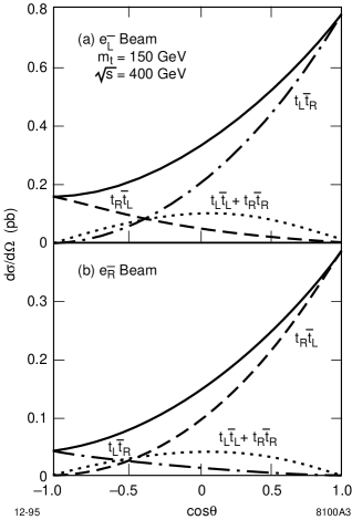
Figure 9: Production angle for $t\bar{t}$ for the possible final-state helicity combinations, as indicated, for (a) left-polarized electrons, and (b) right-polarized electrons. The complete cross sections are the solid curves.

We now outline an analysis[6, 44] to measure or set limits on the complete set of form factors defined in Eqs. 8 and 9. We consider a modest integrated luminosity of 10 fb^-1, $m_{t}=180$ GeV, and $\sqrt{s}=500$ GeV. Electron beam polarization is assumed to be $\pm 80\%$. The decays are assumed to be $t\rightarrow bW$. In general, one needs to distinguish $t$ from $\bar{t}$. The most straightforward method for this is to demand that at least one of the W decays be leptonic, and to use the charge of the lepton as the tag. (One might imagine using other techniques, for example with topological secondary vertex detection one could perhaps distinguish $b$ from $\bar{b}$.) So we assume the following decay chain:

$$t\bar{t}\rightarrow b\bar{b}WW\rightarrow b\bar{b}q\bar{q}^{\prime}\ell\nu,$$ (11)

where $\ell=e,\mu$. The branching fraction for this decay chain is $8/27$.

Now, since the top production and decay information is correlated, it is possible to combine all relevant observables to ensure maximum sensitivity to the couplings. In this study, a likelihood function is used to combine the observables. We use the Monte Carlo generator developed by Schmidt[42], which includes $t\bar{t}(g)$ production to ${\cal O}(\alpha_{s})$. Most significantly, the Monte Carlo correctly includes the helicity information at all stages. The top decay products, including any jets due to hard gluon radiation, must be correctly assigned with good probability. The correct assignments are rather easily arbitrated using the $W$ and top mass constraints. When the effects of initial-state radiation and beamstrahlung are included, it has been shown[40] that the correct event reconstruction can be performed with an efficiency of about 70%. The overall efficiency of the analysis, including branching fractions, reconstruction efficiency, and acceptance, is about 18%.

After simple, phenomenological detection resolution and acceptance functions are applied, the resulting helicity angles (see Fig. 8) are then used to form a likelihood which is the square of the theoretical amplitude for these angles given an assumed set of form factors. Table 4 summarizes some of the results of this analysis. We see that even with a modest integrated luminosity of 10 fb^-1 at $\sqrt{s}=500$ GeV, the sensitivity to the form factors is quite good, at the level of 5–10% relative to SM couplings. In terms of real units, the 90% CL limits for $F_{2A}^{Z}$ of $\pm 0.15$, for example, correspond to a $t$-$Z$ electric dipole moment of $\sim 8\times 10^{-20}$ e-m. Other studies[45, 40, 46] have found similar sensitivities. As discussed above, this limit is in the range of interest for probing new physics. Therefore it is interesting for future studies to quantify the experimental errors which would result from larger data samples than the modest one assumed above.

Table 4: Subset of results from the global form factor analysis described in the text. The upper and lower limits of the couplings in their departures from the SM values are given at 68% and 90% CL. All couplings, each with real and imaginary parts, can be determined in this way. The right-handed charged-current coupling is shown both for unpolarized and 80% left-polarized electron beam, whereas the other results assume 80% left-polarized beam only. $\Im$ is the imaginary part, otherwise the results listed here are for the real parts.

Form Factor	SM Value	Limit	Limit
	(Lowest Order)	68% CL	90% CL
$F_{1R}^{W}(P=0$)	0	$\pm 0.13$	$\pm 0.18$
$F_{1R}^{W}(P=80\%$)	0	$\pm 0.06$	$\pm 0.10$
$F_{1A}^{Z}$	1	$1\pm 0.08$	$1\pm 0.13$
$F_{1V}^{Z}$	1	$1\pm 0.10$	$1\pm 0.16$
$F_{2A}^{\gamma}$	0	$\pm 0.05$	$\pm 0.08$
$F_{2V}^{\gamma}$	0	$\pm 0.07$	${}^{+0.13}_{-0.11}$
$F_{2A}^{Z}$	0	$\pm 0.09$	$\pm 0.15$
$F_{2V}^{Z}$	0	$\pm 0.07$	$\pm 0.10$
$\Im(F_{2A}^{Z})$	0	$\pm 0.06$	$\pm 0.09$

7.2 Helicity Analysis at Hadron Colliders

As discussed above, the Standard Model makes the firm prediction that the $W$ polarization in top decays depends only on $m_{t}$ and $M_{W}$. For $m_{t}=175$ GeV, the fraction of longitudinally polarized $W$’s in top decay is roughly 70%, with the remaining $W$’s being left-hand polarized. This prediction, which is a direct consequence of the Lorentz structure of the $t$-$W$-$b$ vertex, can be tested in the large $t\bar{t}$ samples expected at the Tevatron and LHC. Non-universal top couplings may manifest themselves in a departure of $B(t\rightarrow bW_{\rm long})$ from its expected value.

The $W$ polarization can be measured in lepton + jets final states by analyzing the angular distribution of the charged lepton from the decay $t\rightarrow Wb$ followed by $W\rightarrow l\nu$. The polarization of the $W$ is related to the charged lepton helicity angle $\theta^{*}_{l}$, which is defined to be the emission angle of the lepton in the rest frame of the $W$, with respect to the direction of the $W$ in the rest frame of the top. (It is equivalent to the angle $\chi_{W}$ of Fig. 8.) This angle can be expressed in terms of quantities measured in the lab frame via[47]

$$\cos\theta^{*}_{l}\approx\frac{2m^{2}_{lb}}{m^{2}_{l\nu b}-M_{W}^{2}}-1.$$ (12)

Here $m_{lb}$ is the invariant mass of the charged lepton and the $b$, and $M_{l\nu b}$ is the invariant mass of the lepton, the $b$, and the neutrino, nominally equal to $m_{t}$.

The experimental strategy is to use the constrained fit described in Section 3 to obtain the jet-parton correspondence, which allows one to evaluate the invariant mass combinations. The resulting $\cos\theta^{*}_{l}$ distribution is then fitted to a superposition of $W$ helicity amplitudes in order to extract the fractions of $W_{\rm left}$, $W_{\rm long}$, and $W_{\rm right}$, which contribute to $\cos\theta^{*}_{l}$ like $\frac{1}{4}(1-\cos\theta^{*}_{l})^{2}$, $\frac{1}{2}sin^{2}\theta^{*}_{l}$, and $\frac{1}{4}(1+\cos\theta^{*}_{l})^{2}$ respectively. A model analysis of this type at the Tevatron has been performed by Winn[4]. The $\cos\theta^{*}_{l}$ distribution at the parton level, assuming perfect resolution and no combinatoric misassignments, is shown in Fig. 10. Note that a right-handed component would peak near $\cos\theta^{*}_{l}=1$, where the Standard Model predicts few events.

Figure 10: The parton-level $\cos\theta^{*}_{l}$ distribution for $m_{t}=170$ GeV. The contributions from left-handed and longitudinally polarized $W$’s are shown as the dotted and dashed lines respectively.

To determine best-case statistical precision of this measurement, Monte Carlo[48] pseudo-experiments are performed with top samples of various sizes, still assuming perfect resolution and jet-parton assignment, but correcting the acceptance with a $\cos\theta^{*}_{l}$-dependent factor. A fit to a sample of 1000 events is shown in Fig. 11.

Figure 11: Parton-level, acceptance-corrected $\cos\theta^{*}_{l}$ distribution for 1000 events, together with a fit to the Standard Model hypothesis.

The fit accurately returns the input longitudinal $W$ fraction of 69% to within a 3% statistical uncertainty. The statistical uncertainty in this best-case scenario is found to behave like $1/\sqrt{N}$.

In a real experiment the precision will be lower due to the same effects that complicate the mass measurement: combinatoric misassignment of the top decay products, detector resolution, and backgrounds. The impact of these effects on the helicity analysis has not yet been evaluated in detail. However, since this analysis uses the same constrained fit as the mass measurement, it is reasonable to assume that these effects would be of the same order of magnitude in both analyses. In the mass analysis, these effects lead to a degradation in resolution that is approximately equivalent to a reduction in statistics by a factor of two, i.e. a reduction in precision by a factor of $\sqrt{2}$. If this holds true for the helicity analysis as well, then with a 10 fb^-1 sample at the Tevatron it would be possible to measure the branching fraction to $W_{\rm long}$ to approximately 2%, and to have sensitivity to a right-handed component at the $\approx$1% level.

Neutral-current electroweak couplings of the top quark are not accessible at hadron colliders due to the dominance of strong production mechanisms (or, in the case of single top, production through the weak charged current). Final-state couplings of the top to the photon and $Z$ are extremely small. A study of the neutral-current couplings is therefore the domain of $l^{+}l^{-}$ colliders.

8 The $ttH$ Coupling

The role that the large top mass plays in electroweak symmetry breaking can be directly explored by measuring the top-Higgs Yukawa coupling. In the Standard Model, this coupling strength $\lambda_{t}$ is proportional to the top mass: $\lambda_{t}=2^{1/4}\sqrt{G_{F}}m_{t}$. The top-Higgs coupling is consequently large and can be directly measured. Such measurements are possible at both the LHC and the NLC. The measurements are challenging in both environments, requiring design-level luminosities for adequate statistics.

The process $pp\rightarrow t\bar{t}H+X$ has been studied at the LHC for Higgs masses up to 120 GeV[17]. The process relies on the availability of good vertex detection even at the highest LHC luminosities for efficient $b$-tagging. The Higgs is identified as a bump over a large background in the $bb$ invariant mass distribution in events with a trigger lepton and at least three $b$ jets. The dominant backgrounds are due to $t\bar{t}$ and $W$ production with additional jets, some of which are misidentified as $b$ jets. With 100 fb^-1, signals of more than $3\sigma$ significance are expected for $m_{H}<115$ GeV. In principle this signal could yield a measurement of the top-Higgs coupling, but no such analysis is discussed.

Several techniques can be applied at the NLC. The top coupling to a light Higgs ($m_{H}<2M_{W}$) can be measured at a 500 GeV collider with accurate cross-section measurements at $t\bar{t}$ threshold or by measuring the rate of $t\bar{t}H$ events at $\sqrt{s}=500$ GeV. Higher energies ($\sqrt{s}=1$ or 1.5 TeV) are needed to study the coupling for intermediate or high Higgs mass ($m_{H}>2m_{t}$).

The presence of an additional attractive force arising from Higgs exchange produces a distinctive distortion in the cross section for $t\bar{t}$ production near the 1S resonance. This was discussed in the Section 4.3 above. The size of the distortion is proportional to $\lambda_{t}^{2}/m_{H}$. The coupling could be measured to at least 10% for $m_{H}=100$ GeV with a 100 fb^-1 threshold scan.

The yield of $t\bar{t}H$ events is proportional to the square of the top-Higgs coupling. The cross section for the process is small, of order 1 fb at a 500 GeV NLC for $m_{H}=100$ GeV; it grows to a few fb by 1 TeV[49]. The final state typically contains eight jets, including four $b$ jets. Preliminary studies[10, 30] indicate that $t\bar{t}Z$ and $t\bar{t}jj$ events are significant backgrounds. The top-Higgs coupling could be measured to 25% with 100 fb^-1 if $m_{H}=100$ GeV at $\sqrt{s}=500$ GeV. The accuracy and Higgs mass reach improve at higher energies. For example, Fujii finds a 10% measurement is possible at $\sqrt{s}=700$ GeV with the same integrated luminosity. Studies are needed to quantify sensitivity to intermediate and high mass Higgs at higher $\sqrt{s}$.

The Higgs-strahlung process ($t\bar{t}H$) is also sensitive to effects that might arise from extended Higgs sectors. The interference between Higgs emission from a virtual $Z$ and Higgs-strahlung from the final $t$ quark gives rise to CP-violating effects in two Higgs doublet models. This was studied in Ref. [50] where it was found that CP-violation effects could be seen at $3\sigma$ level with several hundred $t\bar{t}H$ events and the most favorable parameter choices. Such studies will require center of mass energies above 800 GeV and integrated luminosities of 300 fb^-1 or more. Gunion and He presented[51] an analysis to discriminate between different models of the Higgs sector, using two-Higgs-doublet models to exemplify the technique, which consists of measurements of the $t\bar{t}h$ differential cross section together with the $Zh$ total cross section, where $h$ is a neutral Higgs boson. For $m_{h}=100$ GeV, $\sqrt{s}=1000$ GeV, and an integrated luminosity of 500 fb^-1, they find that the Yukawa couplings and Higgs model can be accurately determined.

Measuring the coupling of the top quark to a heavy Higgs ($m_{H}>2m_{t}$) requires high center of mass energies and high intergrated luminosity. Three processes are of interest: $e^{+}e^{-}\rightarrow t\bar{t}H$; $e^{+}e^{-}\rightarrow t\bar{t}Z$; and $e^{+}e^{-}\rightarrow\nu\bar{\nu}t\bar{t}$. Only the latter two have been studied.

The cross-section for $e^{+}e^{-}\rightarrow t\bar{t}Z$ is about 5 fb between 500 and 1000 GeV. It is enhanced by the process $e^{+}e^{-}\rightarrow ZH$ when the Higgs subsequently decays to $t\bar{t}$. For $m_{H}=500$ GeV, the enhancement is about 2 fb at $\sqrt{s}=1000$ GeV. Fujii et al.[29], have studied this process. They enrich their Higgs sample by first requiring a $t\bar{t}Z$ final state, and then cutting on the appropriate $t\bar{t}$ invariant mass. Extrapolating their results to $\sqrt{s}=1000$ GeV and assuming $m_{H}=500$ GeV, leads to an estimated precision in the top-Higgs coupling of 20% for a 100 fb^-1 data set.

Higgs enhancements are more dramatic in the reaction $e^{+}e^{-}\rightarrow\nu\bar{\nu}t\bar{t}$. At $\sqrt{s}=1500$ GeV, the cross-section for this process is about 2 fb in the absence of a Higgs, but will be enhanced by more than a factor of two for Higgs masses in the range 400 to 850 GeV. Peak sensitivities, which occur when $m_{H}=500$ GeV, are nearly 10 times the nominal rate. Preliminary studies by Fujii[29] show that care is required to eliminate radiative $t\bar{t}$, $e^{+}e^{-}t\bar{t}$, and $t\bar{t}Z$ backgrounds. They find that the top Higgs coupling can be measured to 10% with 300 fb^-1 at $\sqrt{s}$ of 1000 GeV for $m_{H}=600$ GeV.

9 Rare and Nonstandard Decays

The search for and discovery of the top quark at Fermilab has relied on the assumption that the standard model decay $t\rightarrow Wb$ dominates. This fact is far from established, of course. In fact, the interesting speculation[52] that a conspiracy of SUSY-enhanced production balancing SUSY-depleted decays explains the observed $t\bar{t}$ signal has not been excluded as yet. The top width is unknown, and present estimates of the branching ratio $t\rightarrow Wb$ are model dependent; so there are only weak experimental constraints on non-standard top decays. The high top mass opens the kinematic window for decays to new, massive states, such as those inspired by supersymmetric models, $t\rightarrow\tilde{t}+$ neutralino ($\chi^{0}$) and $t\rightarrow H^{+}b$. The high top mass also encourages speculation that neutral-current decays, like $t\rightarrow c\gamma$ or $t\rightarrow cZ$, may be large enough to be interesting experimentally. If the stop and neutralino masses are low enough, the decay $t\rightarrow\tilde{t}\chi^{0}$ can occur with a sizable branching fraction. Typically, one imagines that the neutralino escapes undetected and that the subsequent decay, $\tilde{t}\rightarrow c\chi^{0}$, leaves a lone remnant hadronic jet and missing energy. It is reasonable to expect that this issue will be addressed with present and future Fermilab data by searching for events with an identified $t$, a charm jet, and missing energy. Venturi[53] has studied how to detect this decay at an NLC, which is done by looking for an event where the invariant mass of one hemisphere is near the top mass, and the other is substantially below. He finds that a 10 fb^-1 data set is sufficient to establish a 3$\sigma$ discovery, provided the branching fraction is $>2\%$ (for $m_{\tilde{t}}=80$ GeV and $m{\chi^{0}}=55$ GeV).

Top decays to a charged Higgs, $t\rightarrow H^{+}b$, are also expected in supersymmetric models when the decay is kinematically allowed. The charged Higgs is expected to decay predominantly to $\tau\nu_{\tau}$ when $\tan\beta>1$, so the appropriate signature is an apparent violation of lepton universality in top decays, leading to an excess of taus in the top decay products. Run 2 at the Tevatron will be sensitive to branching fractions $B(t\rightarrow H^{+}b)>11\%$[4]. At LHC, the decay is detectable if $m_{H}<130$ GeV for most values of $\tan\beta$ with 10 fb^-1[17]. At NLC a study[53] has shown that the decay is observable if $m_{H}<125$ GeV, essentially independent of the value of $\tan\beta$, with 100 fb^-1.

The FCNC decays $t\rightarrow c\gamma$ and $t\rightarrow cZ$ are tremendously suppressed in the Standard Model, with branching fractions of order $10^{-12}$. Consequently their observation at detectable levels is a robust indication of new physics. Models with singlet quarks or compositeness could have branching ratios for these decays as large as 1%[54]. The signature for these decays, a very high $P_{T}$ photon or a high energy lepton pair with an invariant mass consistent with the $Z$ mass, are distinctive enough to permit sensitive searches in the hadronic environment. Run 2 at the Tevatron will probe to branching fractions of about $3\times 10^{-3}$ ($2\times 10^{-2}$) for $t\rightarrow c\gamma$ ($t\rightarrow cZ$)[4]. At the LHC with its very large top samples, branching fractions as small as $5\times 10^{-5}$ could be measured for $t\rightarrow cZ$, assuming an integrated luminosity of 100 fb^-1[17]. At NLC, the sensitivity is limited by the available statistics to of order 10^-4 for $t\rightarrow c\gamma$ and 10^-3 for $t\rightarrow cZ$, assuming an integrated luminosity of 50 fb^-1. Similar limits could be established by looking directly for $e^{+}e^{-}\rightarrow t\bar{c}$ events[54].

10 Conclusions

The systematic study of the top quark offers many possibilities for exploring physics beyond the standard model. Because the top quark mass enters quadratically into the $\rho$-parameter, a precision measurement of $m_{t}$ can be used together with $M_{W}$ to constrain the Higgs mass. In the exciting event that a Higgs particle is observed, knowledge of $m_{t}$ will help determine whether it is a standard model Higgs or some other, more exotic variety. Measurements of the top couplings and form factors directly probe the weak interactions of a bare quark at their natural scale, and anomalies in these couplings could signal the presence of new physics at the TeV scale or higher. Direct measurements of the top width and $V_{tb}$ could reveal the existence of nonstandard decay modes or additional quark generations. And the top-Higgs Yukawa coupling can be probed directly, particularly if the Higgs is light. Each of these measurements is of great interest and should play an important role in planning future experiments.

The Fermilab Tevatron will be the only facility capable of studying the top quark until the LHC turns on in 2005. With 30 fb^-1 delivered in “Run III” following the initial Main Injector collider run, a top mass uncertainty of ${\rm\raisebox{-3.01385pt}{$\stackrel{{\scriptstyle\textstyle<}}{{\sim}}$}}2$ GeV appears feasible. This measurement would be sufficiently accurate that uncertainties in other quantities ($M_{W}$, $\sin^{2}\theta_{W}$,$\alpha_{s}(M_{Z}^{2})$) would dominate the precision electroweak fits. The Tevatron can measure $\Gamma_{t}$ and $V_{tb}$ to better than 10%, albeit with some model-dependent assumptions. The Tevatron will also test the charged-current form-factors and search for rare and nonstandard decays. Its main advantage, of course, is that it exists and has a monopoly on the subject for roughly the next decade. The Tevatron program should take full advantage of this situation and maximize the integrated luminosity before the LHC turn-on.

The LHC, with its enormous top production cross section, is a veritable top factory. In particular, its sensitivity to rare decays is unlikely to be matched by other machines. As is the case for the Tevatron, many measurements will be systematics-limited. Neither LHC experiment, for example, is currently willing to claim a mass measurement better than 2 GeV. However, the very large control samples that will be available at the LHC suggest that these systematics might be better controlled, or that precision measurements could be performed using small, very clean subsamples. The measurement of the top-Higgs coupling at the LHC will be extremely challenging due to the low cross section and difficult backgrounds. In general, top physics at the LHC has not been studied in the same level of detail as, say, Higgs and SUSY searches. It could benefit from additional study since its potential has not been fully explored.

An $e^{+}e^{-}$ linear collider offers the greatest potential for high-precision top physics in the LHC era. If the beam energy spectrum can be understood to the level expected, the top mass can be measured to better than 200 MeV. A number of fundamental parameters can be measured at the $t\bar{t}$ threshold, including $\Gamma_{t}$, $V_{tb}$, $\alpha_{s}$, the charge and spin of the top quark, and the top-Higgs Yukawa coupling if the Higgs is sufficiently light. The full array of top gauge couplings can be measured, including the neutral-current couplings, which are inaccessible at hadron colliders. The top-Higgs coupling can be measured in the open top region as well, though this will require extended running at design luminosity. If the Higgs (or a Higgs) is light enough for this measurement to be made, it will also be light enough to have been directly observed at the NLC, LHC, or even perhaps the Tevatron. The Yukawa coupling of this particle to the top quark may depend on whether it is a standard model Higgs, a SUSY Higgs, or some other thing entirely. A direct measurement of this coupling will thus address head-on the question of how the top quark, and by extension all fermions, acquire mass.

References

- [1] F. Abe et al. (CDF Collaboration), Phys. Rev. Lett.74,2626 (1995).
- [2] S. Abachi et al. (D0 Collaboration), Phys. Rev. Lett.74, 2632 (1995).
- [3] For a review of the top mass and other measurements, see D. Gerdes, “Top Quark Physics Results from CDF and D0,” these proceedings; hep-ex/9609013 (1996).
- [4] “Future Electroweak Physics at the Fermilab Tevatron: Report of the TEV2000 Study Group,” D. Amidei and R. Brock eds., Fermilab-Pub-96/082 (1996).
- [5] M. E. Peskin and H. Murayama, “Physics Opportunities of Linear Colliders,” Ann. Rev. Nucl. Part. Sci. 46, 533 (1996); hep-ex/9606003 (1996).
- [6] R. Frey, “Top Quark Physics at a Future Linear Collider: Experimental Aspects,” proceedings of the Workshop on Physics and Experiments with Linear Colliders (LCWS95), Iwate, Japan, Sept., 1995; hep-ph/9606201 (1996).
- [7] E. L. Berger and H. Contapaganos, Phys. Rev. D54, 3085 (1996); S. Catani, M. L. Mangano, P. Nason, and L. Trentadue, Phys. Lett. B378, 329 (1996); S. Catani, M. L. Mangano, P. Nason, and L. Trentadue, CERN-TH/96-86, hep-ph/9604351 (1996). E. Laenen, J. Smith, and W. L. Van Neerven, Phys. Lett. B321, 254 (1994).
- [8] S. Dawson, Nucl. Phys. B249, 42 (1985); S. Willenbrock and D. Dicus, Phys. Rev. D34, 155 (1986); S. Dawson and S. Willenbrock, Nucl. Phys. B284, 449 (1987); C.-P. Yuan, Phys. Rev. D41, 42 (1990); S. Cortese and R. Petronzio, Phys. Lett. B253, 494 (1991); G. V. Jikia and S. R. Slabospitsky, Phys. Lett. B295, 136 (1992); R. K. Ellis and S. Parke, Phys. Rev. D46, 3785 (1992); G. Bordes and B. van Eijk, Z. Phys. C57, 81 (1993); G. Bordes and B. van Eijk, Nucl. Phys B435, 23 (1995); D. O. Carlson and C.-P. Yuan, Phys. Lett B306, 386 (1993); T. Stelzer and S. Willenbrock, Phys. Lett. B357, 125 (1995).
- [9] T. Barklow, talk presented at this meeting.
- [10] K. Fujii, T. Matsui, and Y. Sumino, Phys. Rev. D50, 4341 (1994).
- [11] D.J. Jackson, talk presented at this meeting.
- [12] M. Peskin and T. Takeuchi, Phys. Rev. D 46,381 (1992)
- [13] U. Sarid, these proceedings; hep-ph/9610341 (1996).
- [14] P. Tipton for CDF Collaboration, XXVIII International Conference on High Energy Physics, Warsaw, Poland, July, 1996.
- [15] M. Strovink, “The D0 Top Quark Mass Analysis,” to appear in the proceedings of the 11th Topical Workshop on Proton-Antiproton Collider Physics, Padua, Abano Terme, Italy, 26 May - 1 June 1996; FERMILAB-CONF-96/336-E (1996).
- [16] A. Heinson “Future Top Physics at the Tevatron and LHC,” Proceedings of the XXXIst Rencontres de Moriond, QCD and High Energy Hadronic Interactions, Les Arcs, Savoie, France, 23rd-30th March 1996.
- [17] ATLAS Technical Proposal, CERN/LHCC 94-43, LHCC/P2 (1994).
- [18] R. Raja, these proceedings; hep-ex/9609016 (1996).
- [19] L. H. Orr, T. Stelzer, and W.J. Stirling, Phys. Rev. D52, 124 (1995).
- [20] M. Strassler and M. Peskin, Phys. Rev. D43, 1500 (1991).
- [21] V. Fadin and V. Khoze, JETP Lett. 46, 525 (1987) and Sov. J. Nucl. Phys. 48, 309 (1988).
- [22] M. Jezabek, J. Kuhn, and T. Teubner, Z. Phys. C56, 653 (1992).
- [23] M. Jezabek and T. Teubner, Z. Phys. C59, 669 (1993).
- [24] Y. Sumino, K. Fujii, K. Hagiwara, H. Murayama, and C.-K. Ng, Phys. Rev. D47, 56 (1993).
- [25] E.A. Kuraev and V.S. Fadin, Sov. J. Nucl. Phys. 41, 466 (1985).
- [26] Pisin Chen, Phys. Rev. D46, 1186 (1992).
- [27] C. Adolphsen, et al., “Zeroth-Order Design for the NLC”, Ch. 12, SLAC Report 474, May 1996; and references therein.
- [28] P. Igo-Kemenes, M. Martinez, R. Miquel, and S. Orteu, proceedings of the Workshop on Physics and Experiments with Linear Colliders (LCWS93), Waikoloa, Hawaii, USA, 1993.
- [29] K. Fujii, proceedings of the 1995 SLAC Summer Institute.
- [30] P. Comas, R. Miquel, M. Martinez, and S. Orteu, “Recent Studies on Top Quark Physics at NLC”, proceedings of the Workshop on Physics and Experiments with Linear Colliders (LCWS95), 1995.
- [31] R. Harlander, M. Jezabek, and J.H. Kuhn, Acta. Phys. Polon. 27, 1781 (1996), hep-ph/9506292 (1995).
- [32] H. Murayama and Y. Sumino, Phys. Rev. D47, 82 (1993).
- [33] N.M. Frary and D. Miller, DESY 92-123A, Vol. I, 1992, p. 379.
- [34] T. Stelzer and S. Willenbrock, Phys. Lett. B357, 125 (1995).
- [35] T. Stelzer, these proceedings.
- [36] W. Bernreuther and M. Suzuki, Rev. Mod. Phys. 63, 313 (1991).
- [37] W. Bernreuther, T. Schrooder, and T.N. Pham, Phys. Lett. B279, 389 (1992).
- [38] A. Soni and R. Xu, Phys. Rev. Lett. 69, 33 (1992).
- [39] T.G. Rizzo, these proceedings; hep-ph/9610373 (1996).
- [40] G.A. Ladinsky and C.P. Yuan, Phys. Rev. D49, 4415 (1994); see also references therein.
- [41] M.E. Peskin and C.R. Schmidt, proceedings of the Workshop on Physics and Experiments with Linear Colliders (LCWS91), Saariselka, Finland, 1991.
- [42] C.R. Schmidt, SCIPP-95/14 (1995); hep-ph/9504434 (1995).
- [43] S. Parke and Y. Shadmi, Phys. Lett. B387, 199 (1996).
- [44] M. Fero, talk presented at this meeting.
- [45] D. Atwood and A. Soni, Phys. Rev. D45, 2405 (1992).
- [46] F. Cuypers, proceedings of the Workshop on Physics and Experiments with Linear Colliders (LCWS95), 1995.
- [47] G. L. Kane, C. P. Yuan, and G. Ladinsky, Phys. Rev. D45, 124 (1992).
- [48] The event generator used is that of E. Malkawi and C. P. Yuan, Phys. Rev. D50, 4462 (1994).
- [49] A.Djouadi, J. Kalinowski and P.M. Zerwas, Z. Phys. C54, 255 (1992).
- [50] S. Bar-Shalom, D. Atwood, G. Eilam, R. Mendel, and A. Soni, Phys. Rev. D53, 1162 (1996).
- [51] J.F. Gunion and X.-G. He, these proceedings; hep-ph/9609453 (1996).
- [52] G. L. Kane and S. Mrenna, Phys. Rev. Lett 77, 3502 (1996).
- [53] A. Venturi, in proceedings of the Workshop on Physics and Experiments with Linear Colliders (LCWS93), Waikoloa, Hawaii, USA, 1993.
- [54] T. Han and J. Hewett, SLAC-PUB-7178, Dec. 1996.