LU TP 97/06

hep-ph/9704233

April 1997

Chiral Perturbation Theory and Threshold Corrections
Johan Bijnens
Department of Theoretical Physics, University of Lund,

Sölvegatan 14A, S 223 62 Lund, Sweden

I give a short overview of Chiral Perturbation Theory, its underlying assumptions and underpinnings. A few examples are included.

1 Introduction

In this talk I will give a short introduction to Chiral symmetry and the Goldstone theorem. These we then combine into Chiral Perturbation Theory(CHPT). This is a systematic tool to solve the Ward identities of Chiral symmetry. Its main advantage over the use of models is that it is a theory, i.e. higher order corrections can in principle be calculated and the convergence of the expansion tested. It is also systematic, there are no hidden assumptions. $\pi\pi$ scattering will be used as an example here.

We will then go beyond PCAC and show more examples, $\gamma\gamma\to\pi^{+}\pi^{-}$ where a naive estimate would have worked and $\gamma\gamma\to\pi^{0}\pi^{0}$ where the naive expectation did not work.

The last section is an extremely short review of pion photoproduction. This is mainly the work of V. Bernard et al..

2 Chiral Symmetry

2.1 Definition and Goldstone Theorem

In Quantum Chromodynamics (QCD) we have quarks, if they have the same (or nearly the same) mass we have a symmetry by interchanging them. For the case of two flavours this is known as isospin. It is a continuous symmetry, $SU(2)_{V}$. A generalization to three flavours is the Gell-Mann-Okubo eightfold way where the symmetry is enlarged to $SU(3)$.

In the case of massless particles this symmetry is larger. The underlying reason is that left and right handed particles are really distinct entities. As shown in Fig. 1 by overtaking a massive particle you change the direction of its momentum but not of its angular momentum. So you flip its helicity. Since you cannot overtake a massless particle the two helicities are fully separate.

Figure 1: Lorentztransformations couple left and right helicities for massive particles by changing the sign of he momentum. This is not possible for massless particles.

As a consequence isospin gets doubled to the chiral symmetry group $SU(2)_{L}\times SU(2)_{R}$ with a separate “isospin” for both helicities. In the case of 3 massless flavours the symmetry group is $SU(3)_{L}\times SU(3)_{R}$.

This symmetry group is however not manifest in nature at all. E.g., the parity partners vector mesons $a_{1}$ and $\rho$ have masses of 1230 MeV and 770 MeV respectively, the proton-neutron and their partners, the $S_{11}$, have masses of about 940 MeV versus 1535 MeV. So the question is: where is the symmetry ?

The Wigner-Eckart theorem we all learned in our quantum mechanics course has a loophole, the Goldstone theorem uses this loophole. The usual proof of the Wigner-Eckart theorem assumes that the vacuum, or lowest energy state, is unique. Once we drop this requirement, the Wigner-Eckart theorem is no longer valid. Let me show it in a somewhat schematic way. For a symmetry generated by $Q$ we have two related states, $\alpha$ created by the creation operator $a^{\dagger}$ and $\beta$ created by $b^{\dagger}=e^{i\gamma Q}a^{\dagger}e^{-i\gamma Q}$. $Q$ and $e^{i\gamma Q}$ commute with the Hamiltonian $H$ since it generates a symmetry. Then:

$$m_{\beta} = \langle 0|bHb^{\dagger}|o\rangle$$ (1)

$$= \langle 0|e^{i\gamma Q}ae^{-i\gamma Q}He^{i\gamma Q}a^{\dagger}e^{-i\gamma Q}|0\rangle$$

$$= \langle 0|e^{i\gamma Q}aHa^{\dagger}e^{-i\gamma Q}|0\rangle$$

$$\mbox{if }Q|0\rangle=|0\rangle\mbox{, the vacuum is a singlet under the symmetry}$$

$$= \langle 0|aHa^{\dagger}|0\rangle$$

$$= m_{\alpha}$$

So if there are several vacua we can have a symmetry group and $m_{\alpha}\neq m_{\beta}$.

The underlying symmetry still has lots of consequences. See [1]. A naive proof goes as follows:
If you have a continuous symmetry generated by a generator $Q$. The effect of the other vacua that have to be chosen at each point in space time can be described by a field $\phi(x)$. The vacuum in a point $x$ is given by $\displaystyle e^{i\phi(x)Q}|0\rangle$ where $|0\rangle$ is a reference vacuum. The symmetry is still a global symmetry, so a rotation that is the same in all space time cannot do anything. So $\displaystyle e^{i\phi(x)Q}|0\rangle$ and $\displaystyle e^{i(\phi(x)+\alpha)Q}|0\rangle$ describe the same state. The Lagrangian (or more precisely the action) should be the same for $\phi(x)$ and $\phi(x)+\alpha$ with $\alpha$ a constant. The dependence on the field $\phi$ can thus only happen via derivatives or $\phi$ can only occur as $\partial_{\mu}\phi$. Thus mass terms are excluded and interactions vanish at zero energy and momentum. The massless particle described by $\phi$ is called a Goldstone boson.

2.2 Chiral Perturbation Theory

For CHPT we use the Goldstone theorem for the chiral symmetry. The symmetry which is broken is the axial part of the chiral symmetry. The diagonal vector subgroup remains unbroken. For $N_{f}$ flavours this means that there are $N_{f}^{2}-1$ broken symmetries or we will get $N_{f}^{2}-1$ Goldstone bosons. The interactions are weak at low energies. We can therefore do a systematic expansion in the number of derivatives and have a well defined, consistent perturbation theory. In the case of two flavours we can define a four-vector $\vec{U}$ containing the 3 Goldstone bosons $\pi^{i}$ and a lowest order Lagrangian:

$$\vec{U} = \left(\sqrt{1-\frac{\vec{\pi}^{2}}{F^{2}}},\frac{\pi^{1}}{F},\frac{\pi^{2}}{F},\frac{\pi^{3}}{F}\right)$$

$$\vec{\chi} = 2B\left(s^{0},p^{i}\right)$$

$${\cal L}_{2} = \frac{F^{2}}{4}\left(\nabla_{\mu}\vec{U}\cdot\nabla^{\mu}\vec{U}+\vec{\chi}\cdot\vec{U}\right)\,.{}$$ (2)

The covariant derivative $\nabla_{\mu}$ is defined in [3]. The field $\chi$ contains the quark masses. The extension to 3 flavours is in [4]. This Lagrangian contains at tree level a very large part of all the PCAC predictions of the sixties. The reason for using external fields is explained in [3, 4]. For a simple example explaining the advantage see [5].

2.3 Powercounting and $\pi\pi$-scattering.

As argued in the previous subsection we have a well defined expansion in terms of derivatives (and quark masses). This was proven in a simple way in Weinberg’s paper[6]. Let us show the arguments at the example of $\pi\pi$ scattering. The classes of diagrams are shown in Fig. 2.

Figure 2: Some diagrams contributing to $\pi\pi$ scattering.

A vertex contains two derivatives, so two powers of momenta, $p^{2}$, a propagator is the inverse of the kinetic term, it has dimension $-$2, or $p^{-2}$ and a loop integral, $d^{4}p$, has dimension 4 or $p^{4}$. The lowest order term of Fig. 2a is order $p^{2}$. The loop diagrams of (b) and (c) are $p^{4}$ and the two-loop diagram of (e) is $p^{6}$. The convergence of this expansion works quite well. The lowest order[7], the $p^{4}$[3] and the $p^{6}$ calculation[8] converge up to about 500 MeV or so. The combination measurable in $K_{l4}$ decays is shown in Fig. 3. The data are from [9].

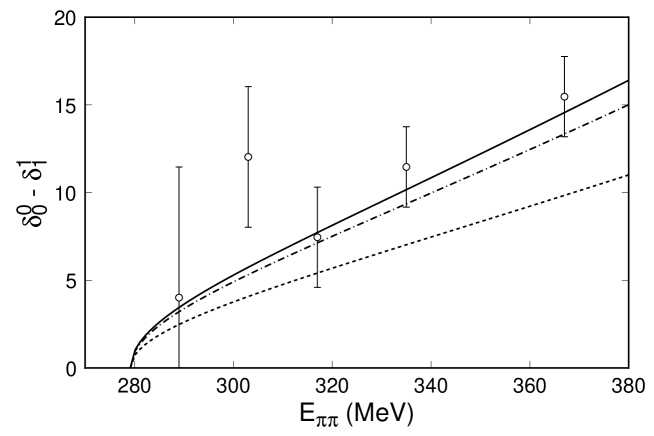
Figure 3: The $\pi\pi$-phase shift measurable in $K_{l4}$ together with the CHPT results[8].

We can also look at one of the scattering lengths at threshold to see the convergence:

$$a^{0}_{0} = 0.156(\mbox{tree})+\overbrace{0.039(L)+0.005(\mbox{anal})}^{\mbox{1-loop}}$$ (3)

$$+\overbrace{0.013(L^{2}+l_{i}L)+0.003(L)+0.001(\mbox{anal})}^{\mbox{2-loop}}\,.$$

Here the first term is the tree level. The symbol $L$ stands for the nonanalytic contribution proportional to $L=\log(m_{\pi}^{2}/\mu^{2})$, $L^{2}$ for those proportional to the square and $l_{i}L$ for the one-loop contributions with a $p^{4}$-vertex in the diagram. The unknown $p^{6}$ coefficients only contribute to the last term. In this particular case the nonanalytic pieces dominate so the uncertainty due to higher order terms is rather small.

3 Examples

3.1 $\gamma\gamma\to\pi^{+}\pi^{-}$

This is a process where everything works as we expect. The Born term is just scalar electro dynamics and dominates the cross section within the whole domain of validity of CHPT. The $p^{4}$ part[10] gives a reasonable correction and the $p^{6}$ calculation [11] has even smaller effects. See the figures in [11].

3.2 $\gamma\gamma\to\pi^{0}\pi^{0}$

If we would have been naive we would have said: There are no terms in the action contributing to order $p^{2}$ and $p^{4}$ (this was known as the Veltman-Sutherland theorem) but there are terms of order $p^{6}$. An order of magnitude estimate of their coefficient would lead to a cross section of order 0.04 nb. However the nonanalytic pieces are nonzero at order $p^{4}$[10, 12] and give a cross section of a few nanobarn. This agreed roughly with the measurements. The $p^{6}$ corrections were later calculated and still found to be significant[13]. See Fig. 4.

Figure 4: The cross section $\gamma\gamma\to\pi^{0}\pi^{0}$. Dashed line is $p^{4}$, full line $p^{6}$ and the crosses the data[14]. Figure taken from [13].

So, the Low Energy Theorem was wrong, the amplitude is nonanalytic and the loops gave the correct order of magnitude. So why were there still very large $p^{6}$ corrections ?

The reason is that the underlying isospin amplitudes, I=0,2, are both very large. For the charged pion production they add up so we only find moderate corrections to the total. For the neutral pion production they cancel, but they have different higher order corrections, I=0 has large rescattering effects, I=2 has not. Differences of large numbers tend to be much more sensitive to higher orders.

4 Pion Photoproduction

Similar effects as described in the previous section happen here. For $E_{0+}$ in $\gamma p\to\pi^{0}p$ there was a similar wrong low energy theorem[15]. All higher order corrections up to $p^{4}$ have by now been calculated by the group of Bernard, Kaiser and Meißner. Examples of badly converging, like $E_{0+}$ in neutral, and well converging quantities, like most quantities in charged pion photoproduction, can all be found. In the talk I presented the examples but much more detailed discussions can be found in [16].

5 Conclusions

Chiral perturbation provides a well defined framework for low energy hadronic physics. It cleanly separates model aspects, which here are estimates of the constants, from the basic aspects of chiral symmetry. It is very successful in describing the data in its regimes of applicability. However it should be kept in mind that it is a perturbative low energy expansion. At higher energies we can still use the principles of CHPT for organizing our thoughts but we should beware of numerical results.

References

- [1] J. Goldstone, Nuovo Cim. 19 (1961) 154, for an introduction see e.g. [2].
- [2] J. Donoghue, E. Golowich and B. Holstein, Dynamics of the Standard Model, Cambridge University Press, 1992.
- [3] J. Gasser and H. Leutwyler, Ann. of Phys. 158 (1984) 142.
- [4] J. Gasser and H. Leutwyler, Nucl. Phys. B250 (1985) 465.
- [5] J. Bijnens, Chiral perturbation Theory in Chiral Dynamics in Hadrons and Nuclei, eds. D.P.Min and M. Rho, Seoul National University Press, 1995, hep-ph/9502393.
- [6] S. Weinberg, Physica 96A (1979) 327.
- [7] S. Weinberg, Phys. Rev. Lett. 17 (1966) 616.
- [8] J. Bijnens et al., Phys. Lett. B374 (1996) 210.
- [9] L. Rosselet et al., Phys. Rev. D15 (1977) 574.
- [10] J. Bijnens and F. Cornet, Nucl. Phys. B296 (1988) 557.
- [11] U. Burgi, Phys. Lett. B377 (1996) 147, Nucl. Phys. B479 (1996) 392.
- [12] J. Donoghue, B. Holstein and Y. Lin, Phys. Rev. D37 (1988) 2423.
- [13] S. Bellucci, J. Gasser and M. Sainio, Nucl. Phys. B423 (1994) 80.
- [14] H. Marsiske et al., Phys. Rev. D41 (1990) 3324.
- [15] V. Bernard et al., Phys. Lett. B268 (1991) 291.
- [16] V. Bernard, N. Kaiser and U.-G. Meißner, Phys. Lett. B378 (1996) 337, Int. J. Mod. Phys. E4 (1995) 193 (review), Phys. Rept. 246 (1994) 315.