Abstract

In this paper we make predictions for nondiagonal parton distributions in a proton in the LLA. We calculate the DGLAP-type evolution kernels in the LLA, solve the nondiagonal GLAP evolution equations with a modified version of the CTEQ-package and comment on the range of applicability of the LLA in the asymmetric regime. We show that the nondiagonal gluon distribution $g(x_{1},x_{2},t,\mu^{2})$ can be well approximated at small $x$ by the conventional gluon density $xG(x,\mu^{2})$.
PACS: 12.38.Bx, 13.85.Fb, 13.85.Ni
Keywords: Hard Diffractive Scattering, Nondiagonal distributions, Evolution

I Introduction

Due to the experimental possibility of probing nondiagonal distributions in hard diffractive electro-production processes, theoretical interest in this area in recent years [1, 2, 3, 4, 5, 6, 7] has produced interesting results. A pioneering analysis of the nondiagonal distributions for the diffractive photoproduction of $Z^{0}$-bosons in DIS where the applicability of PQCD is guaranteed was given by Bartels and Loewe in 1982 [8] but went essentially unnoticed.

In the this paper we would like to complement these results by concrete predictions, albeit to the LLA, which can be tested by an experiment. In Sec. II we shall demonstrate that in the limit of small $x$ the amplitudes of hard diffractive processes can be calculated in terms of discontinuities of nondiagonal parton distributions. The real part of the amplitude will be calculated by applying a dispersion representation of the amplitude over $x$. We will show that the term in the amplitude which cannot be calculated in terms of the discontinuities of nondiagonal parton distributions [3, 4] is suppressed by one power of $x$ in this limit. This result will make it possible to calculate the evolution kernels in the LLA following the traditional methods [9] and to compare them to results obtained in the QCD-string operator approach [10].

In Sec. III we calculate the nondiagonal kernels and find them equivalent to those in [3, 5]. They are different from the evolution equations for nondiagonal parton densities which were presented without derivation in [11]. In Sec. IV we shall make predictions about the nondiagonal parton distributions by solving, numerically, the nondiagonal GLAP evolution equations with the help of a modified version of the CTEQ-package. In Sec. V we shall discuss the limitations of the approximation and the need for NLO-results. Future directions will be discussed in the conclusions.

II Nondiagonal parton distributions and hard diffractive processes.

It has been recently understood that the major difference in QCD between leading twist effects in DIS and higher-twist effects in hard diffractive processes is to be attributed to the fact that the latter, initiated by highly virtual, longitudinally polarized photons, can be calculated in terms of nondiagonal, rather than diagonal, parton distributions [7].

Thus, in order to calculate unambiguously hard two-body processes, it is necessary to calculate nondiagonal parton distributions in a nucleon. This implies knowledge of the non-perturbative nondiagonal parton distributions in the nucleon which have not been measured so far. Hence, the aim of this section is to express the nondiagonal parton distributions in the nucleon through quantities being maximally close to the diagonal parton distributions. Our second aim is to elucidate on the kinematics of the nondiagonal parton distributions in the nucleon needed to describe hard diffractive processes. We shall also discuss the expected, limiting, behaviour of the nondiagonal parton distributions.

For the leading twist effects QCD evolution equations have traditionally been discussed in terms of the imaginary part of the amplitude. This is because the bulk of experimental data available is on the total cross sections of inclusive processes. However it is well known that the QCD evolution equation has a simple form for the whole amplitude which includes both real and imaginary parts [12]. This form of the evolution equation can be generalized to the case of higher-twist processes, hard diffractive processes [2] and hard two-body processes[4]. The analysis of the QCD evolution equation for the nondiagonal parton densities shows that the evolution equation contains two terms. The first one is described by a DGLAP-type evolution equation[2, 3, 4, 7], whereas the second term, found in Ref. [3] for vector meson production at small $x$, cannot be interpreted in terms of parton distributions. The QCD evolution of this term is governed by the Brodsky-Lepage evolution equation [3, 6].

A GLAP evolution equation for hard diffractive processes

The aim of this section is to prove that for hard diffractive processes in general, the $Q^{2}$-evolution at any $x$ in the DGLAP-region as discussed below, is described by a nondiagonal GLAP-type evolution equation with asymmetric DGLAP-type kernels and that these processes can be calculated through the discontinuity of hard amplitudes. This property is important for the quantitative calculations since the dispersive contribution has a relatively simple physical interpretation and a deep relation with the conventional parton densities. As to the first step, we shall deduce a relationship between amplitudes of hard two-body processes and parton densities, and we will find an additional term which has no probabilistic interpretation. We will restrict ourselves to the $Q^{2}$-region where the parton distributions are still rising and the additional term is of no importance as discussed below.

The QCD factorization theorem for hard processes means that the hard blob can be factorized from the soft one with a precision of a power of $Q^{2}$. The topologically dominant Feynman diagrams for small $x$ processes correspond to attachments of only two gluons to the hard blob. Although our analysis is rather general, for certainty we shall restrict ourselves to the case of diffractive processes where diagrams with two-gluon exchange dominate. It is convenient to decompose the momentum of the exchanged gluon $k$ in Sudakov-type variables:

$$k=x_{1}\tilde{p}+\beta\tilde{q}+k_{t},$$ (1)

where

$$\tilde{p}^{2}=\tilde{q}^{2}=0\ \ \mbox{and}\ \ (k_{t}q)=(k_{t}p)=0.$$ (2)

To express the amplitude in terms of non-diagonal parton distributions, the contour of integration over $\beta$ should be closed over the singularities of the amplitude in gluon-nucleon scattering at fixed $x_{1}$ and $x_{1}-x$. The singularities over $\beta$ are located in the complex plane of discontinuities over the gluon virtualities: ${i\epsilon\over x_{1}}$ and ${i\epsilon\over x_{1}-x}$, and from the $s$- and $u$- channel discontinuities: ${-i\epsilon\over(1-x_{1})}$ and ${i\epsilon\over(1+x_{1}-x)}$. The amplitude differs from 0 if these singularities pinch the contour of integration. This causality condition restricts the region of integration to:

$$-1+x\leq x_{1}\leq 1.$$ (3)

Our main interest is in the amplitude in the physical region where $-t\geq 0$ but small as compared to other relevant scales of the process under consideration. In this region the amplitude can be represented as the sum of terms having $s$- or $u$-channel singularities only. For the $s$-channel contribution to the amplitude of hard diffractive processes, given $1\geq x_{1}\geq x$, the integral over $\beta$ can only be closed over the discontinuity in the amplitude of the gluon-nucleon scattering in the variable $s$.

Thus this contribution to the amplitude is expressed through the imaginary part of the amplitude for gluon-nucleon scattering. The QCD evolution of this term is described by a GLAP-type evolution equation where the kernel accounts for the off-diagonal kinematics. One also has to add a similar term corresponding to $u$-channel singularities.

The contribution of the region $x\geq x_{1}\geq 0$ has no direct relationship to the conventional parton densities. This is because the integral over $\beta$ cannot be closed for $s$- or $u$-channel discontinuities but it may be closed for the discontinuities over the gluon ”mass”. In Ref. [3] the analogy of this term with the wave function of a vector meson has been suggested. The presence of this piece which cannot be evaluated in terms of parton densities introduces theoretical uncertainties into the treatment of hard two-body processes at large and moderate $x$.

However, for the imaginary part of the amplitude, more severe restrictions on the region of integration apply:

$$1\geq x_{1}\geq x.$$ (4)

In order to ensure that we have not included any superfluous regions of integration, we consider the discontinuity of the hard amplitude in the $s$- channel. This additional restriction follows from the requirement that the mass of a $q\bar{q}$ system in the intermediate state should be larger than the mass of a produced vector meson such that the hadron cannot decay into the $q\bar{q}$ system. This result helps to prove that the piece which cannot be evaluated in terms of parton densities is inessential for hard diffractive processes. Let us now apply a dispersion representation over the variable $s$. The only term which cannot be reconstructed in terms of a dispersion relation, i.e in terms of discontinuities of parton densities, is the subtraction constant in the real part. The contribution of the subtraction term to the amplitude with a positive signature, i.e symmetric under the transposition of $s\rightarrow u$, is suppressed by an additional power of $s$ or, equivalently, by an additional power of $x$. For the processes with negative charge parity in the crossed channel, i.e. electroproduction of a neutral pion, the amplitude is antisymmetric under the transposition $s\rightarrow u$. This amplitude has no subtraction terms at all, since, in QCD, it increases with energy slower than s. Thus, in this case, a dispersion representation gives the full description. To summarize let us point out once more that the small $x$ behaviour of hard diffractive processes is described through the discontinuities of hard amplitudes.

B Small $x_{i}$ behaviour of the nondiagonal gluon distribution

We want to stress that the slope of the $x$ dependence of the amplitudes for diffractive processes, however not their residue, should be independent of the asymmetry between fractions $x_{1}$ and $x_{2}$ of the nucleon momentum carried by the initial and final gluons. This is due to the fact that the $x_{i}$ of the partons in the ladder are essential , but not the external $x$, and increase with the length of the parton ladder. Hence, the asymmetry between the gluons may be important in one or two rungs of the ladder but not in the whole ladder. Therefore, at sufficiently small $x$, it is legitimate to neglect $x$ in most of the rungs of the ladder as compared to the $x_{i}$. This means that the asymmetry between the gluons influences the residue but not the slope of the $x$ dependence.

Let us now discuss the small $x_{i}$ behaviour of $g(x_{1},x_{2})$ – the nondiagonal gluon density in a nucleon. The factorization theorem – Eq. 3 of [4]– is the basis for the formal definition of the nondiagonal gluon density as the matrix element of gauge-invariant bilocal operators (cf. eq. 6 of [4]):

$$g_{g/p}(x_{1},x_{2},t,\mu) = -\int_{-\infty}^{\infty}\frac{dy^{-}}{4\pi}\,\frac{1}{p_{+}^{2}}\;e^{-ix_{2}p^{+}y^{-}}\langle p^{\prime}|\;TG_{\nu}{}^{+}(0,y^{-},{\bf 0}_{T})\,{\cal P}\,G^{\nu+}(0)\;|p\rangle.$$ (5)

Here $\cal P$ is a path ordered exponential of a gluon field along the light-like line joining the two gluon operators, $t$ is the square of invariant momentum transferred to the target, and $\mu$ describes the scale dependence. The sum over transverse gluon polarizations is implied. Actually Eq. 5 coincides with the definition given in [3, 4] for the same quantity.

For $x_{1}=x_{2}$, $g_{g/p}(x_{1},x_{2})$ is related to the diagonal gluon distribution as $xG_{{\rm diag}}(x)=g_{{\rm nondiag}}(x,x)$. Within the leading $\alpha_{s}\ln x$ approximation where the difference between $\ln x_{i}$ and $\ln x$ can be neglected, this distribution coincides with the diagonal one [1]:

$$G_{{\rm leading\,\alpha_{s}\ln x}}(x_{1},x_{2},t,\mu^{2})=xG(x,\mu^{2}).$$ (6)

We want to stress here that at fixed Bjorken variable $x$, the cross sections of hard diffractive processes are expressed through $g(x_{1},x_{2},t,\mu^{2})$ where $x_{1}-x_{2}=x$. This can be proved by calculating the high energy limit of hard diffractive processes and then applying Ward identities similar to Ref. [1]. This means that the region of integration near $x_{2}=0$ ($x_{2}\ll x_{1}$) gives only a small contribution to the amplitudes of hard diffractive processes.

Alternatively, one can examine the leading regions of the integrals in the calculation of the distribution of a parton in a parton which is imperative in finding the correct hard scattering coefficients for the desired process. This calculation is necessary since one has not only ultraviolet divergences in the partonic cross sections from which one wants to extract the Wilson coefficients, but also infrared divergences stemming from initial-state collinearities of the participating partons (see Ref. [14] for further details) which are cancelled by the perturbatively calculated expansion of the parton distribution. The region of $x_{2}=0$ does not give a leading contribution. This can be seen by using a simple argument that proper Feynman diagrams have no singularity at $x_{2}=0$, and the region of integration over the exchanged gluon momenta $x_{2}=0$ forms an insignificant part of the permitted phase volume.

In the first step one has to show that a gluon with $x_{2}=0$ corresponds to a soft gluon and then one can use the argument by Collins and Sterman [15] first introduced for proving factorization in inclusive $e^{+}e^{-}$-reactions:

• For clarification, the quark-loop to which the gluons attach consists both of the hard part and the part whose momenta are parallel to the vector meson and of the order ${\nu\over m_{N}}={2qp_{N}\over m_{N}}$.

• The minus component $l_{-}$ of the quark-loop which is transferred to the target proton is $l_{-}\approx m_{N}x$. The minus component of the gluon momentum $k$ is:

  $$k_{-}\simeq\frac{(m_{q\bar{q}}^{2}+M_{V}^{2})m_{N}}{2qp_{N}}\ll l_{-},$$ (7)

  where $m_{q\bar{q}}$ is the mass of the $q\bar{q}$ system. Thus we can neglect $k_{-}$ with respect to $l_{-}$ in the calculation of the leading term of the amplitude corresponding to the leading power in the energy of the process.

• The transverse momentum in the quark loop ($l_{t}$) is cut off by the vector meson wave function and thus $l_{t}^{2}\ll Q^{2}$ in stark contrast to DIS, whereas the $k_{t}^{2}$ of the gluon is only restricted by the virtualities in the photon wave function which can be as high as $Q^{2}$ . However one has to satisfy the Ward-identity $k_{\mu}T^{\mu\nu}=0$ where $T$ stands for the amplitude. Using Sudakov-variables this becomes:

  $$x_{2}p_{\mu}T^{\mu\nu}+k_{t\mu}T^{\mu\nu}=0,$$ (8)

  thus for $x_{2}\rightarrow 0$ the transverse momentum of the gluon is very small and can be safely neglected as compared to $l_{t}$.

• One concludes from the above said that the $x_{2}=0$ region corresponds to a soft gluon ($k^{2}\sim 0$) and we can use the argument by Collins and Sterman.

Keeping the above said in mind, the $k$-integral involved in the determination of the leading regions is of the form (up to overall factors):

$$\int_{soft\,k}d^{4}k\frac{1}{((l-k)^{2}+i\epsilon)(k^{2}+i\epsilon)}f(l-k,p)$$ (9)

$$\simeq\int_{soft\,k}dk_{+}\frac{1}{((l_{+}-k_{+})l_{-}-l^{2}_{t}+i\epsilon)(2k_{+}k_{-}-k^{2}_{t}+i\epsilon)}f(l-k,p),$$ (10)

where $f(l-k,p)$ is the amplitude of gluon-nucleon scattering and the integrals over $k_{-}$ and $k_{t}^{2}$ are suppressed for convenience. If one now integrates over the remaining $k_{+}$ momentum one will have the following situations:

• $k_{+}k_{-}\geq k^{2}_{t}$: There are no obstructions in the deformation of the integration contour since $l_{t}\gg k_{t}$ and therefore the pole at $k^{2}=0$ is far from the region of integration allowed in the LLA. In other words this region does not give a leading contribution.

• $k_{+}k_{-}\ll k^{2}_{t}$: There are no obstructions to the contour deformation since $l_{t}\gg k_{t}$ or in other words $k_{+}k_{-}$ can be neglected as compared to $k_{t}^{2}$ since the singularities do not pinch the contour of integration. Thus this region does not give a leading contribution either.

Thus one has proved that if one of the gluons attaching the soft to the hard part has $x_{2}=0$, it will be soft and thus, according to the above reasoning, the $x_{2}=0$ region of integration does not give a leading contribution to the parton distribution.

III Kernels in the LLA

There are several possible ways of calculating the evolution kernels to leading order in QCD. We first used the traditional approach of calculating the evolution kernels in the LLA, via the method of decay cells of e.g., a quark decaying into a quark [16] and using cut-diagram techniques to calculate the appropriate Feynman graphs.

As a cross-check we calculated the first order corrections to the bi-local quark and gluon operators on the light-cone, which not only yielded the nondiagonal kernels for the DGLAP equation but also the nondiagonal Brodsky-Lepage kernels since we were calculating the whole amplitude, not only its imaginary part. However, since we are not interested in those kernels at the moment we will not comment on this fact further, let it be said though that our results on the Brodsky-Lepage kernels agree with those of Ref. [5, 6].

We performed the calculation of the cross-check in a planar gauge i.e $q^{\prime}\cdot A=0$ with $q^{\prime 2}\neq 0$ and used once more Sudakov-variables:

$$k=\beta p^{\prime}+\alpha q^{\prime}+k_{t},$$ (11)

where

$$p^{\prime 2}=q^{\prime 2}=0\ \ \mbox{and}\ \ (k_{t}q)=(k_{t}p)=0.$$ (12)

Since one is neglecting the proton mass one can set $p^{\prime}=P$ where $P$ is the proton momentum.

The insertion of the appropriate bi-local operators for quarks and gluons on the light cone into the Feynman graphs for first order corrections to those operators, short circuits the $+$-momentum in the graph, which means that the loop variable $k$ has not $+$-momentum $\beta P$ but rather $x_{1}P$ (see [14] for more details on calculating one loop corrections to parton dsitributions.). This fact eliviates us from the duty of taking the integral over $\beta$. In the calculation of the kernels, it remains to take the integral over $\alpha$ which can be done by taking the residues and then isolating the leading term multiplying $dk^{2}_{t}/k^{2}_{t}$ and the tree level amplitude. This will then yield the kernels in the leading logarithmic approximation.

In the integral over $\alpha$, one finds three different residues. Two residues stemming from the vertical quark or gluon propagators which yield $\alpha=\frac{k^{2}_{t}}{x_{1}s}$ and $\alpha=\frac{k^{2}_{t}}{x_{2}s}$ giving a contribution in the Brodsky-Lepage region, i.e the Brodsky-Lepage kernels, and one stemming from the horizontal propagator yielding $\alpha=\frac{k^{2}_{t}}{(y_{1}-x_{1})s}$ which contributes to the DGLAP region, i.e the DGLAP kernels. This is analogous to the statements made in Sec. II.

After having taken proper care of the definitions of our quark and gluon distributions in the amplitudes, we find the following expressions for the nondiagonal evolution kernels, where $\Delta$ is given by $x_{1}-x_{2}$ and corresponds to $x_{B_{j}}$ of e.g., vector-meson production. For the quark $\rightarrow$ quark transition we get:

$$P_{qq}(x_{1},\Delta)=\frac{\alpha_{s}}{\pi}2C_{f}\left[\frac{x_{1}+x_{1}^{3}-\Delta(x_{1}+x_{1}^{2})}{(1-\Delta)(1-x_{1})}-\delta(1-x_{1})\left[\int^{1}_{0}\frac{dz_{1}}{z_{1}}+\int^{1}_{0}\frac{dz_{2}}{z_{2}}-\frac{3}{2}\right]\right],$$ (13)

The other kernels are computed the same way from the appropriate diagrams:

$$P_{qg}(x_{1},\Delta) = \frac{\alpha_{s}}{\pi}N_{F}\frac{[x_{1}^{3}+x_{1}(1-x_{1})^{2}-x_{1}^{2}\Delta]}{(1-\Delta)^{2}},$$ (14)

$$P_{gq}(x_{1},\Delta) = \frac{\alpha_{s}}{\pi}C_{F}\frac{[1+(1-x_{1})^{2}-\Delta]}{1-\Delta},$$ (15)

$$P_{gg}(x_{1},\Delta) = 2N_{c}[\frac{(1-x_{1})^{2}+(\frac{1}{2}-x_{1}^{2})(x_{1}-\Delta)}{(1-\Delta)^{2}}-\frac{1}{2}-\frac{x_{1}}{2}+\frac{1}{2}\frac{1}{1-x_{1}}+\frac{1}{2}\frac{x_{1}-\Delta}{(1-x_{1})(1-\Delta)}$$ (17)

$$+\delta(1-x_{1})\left[\frac{\beta_{0}}{4N_{C}}-\frac{1}{2}\int^{1}_{0}\frac{dz_{1}}{z_{1}}-\frac{1}{2}\int^{1}_{0}\frac{dz_{2}}{z_{2}}\right]].$$

A word conccerning our regularization prescription is in order. In convoluting the above kernels, after appropriate scaling of $x_{1}$ and $\Delta$ with $y_{1}$, with a nondiagonal parton density, one has to replace $z_{1}$ and $z_{2}$ in the regularization integrals with $z_{1}\rightarrow(y_{1}-x_{1})/y_{1}$ and $z_{2}\rightarrow(y_{1}-\Delta)/(y_{1}-x_{1})$. This leads to the following regularization prescription as employed in the modified version in the CTEQ package in the next section and in agreement with Ref. [6]:

$$\int^{1}_{x_{1}}\frac{dy_{1}}{y_{1}}\frac{f(y_{1})}{1-x_{1}/y_{1}}_{+} = \int^{1}_{x_{1}}\frac{dy_{1}}{y_{1}}\frac{y_{1}f(y_{1})-x_{1}f(x_{1})}{y_{1}-x_{1}}+f(x)\ln(1-x_{1})$$ (18)

$$\int^{1}_{x_{1}}dy_{1}\frac{(x_{1}-\Delta)f(y_{1})}{(y_{1}-x_{1})(y_{1}-\Delta)}_{+} = \int^{1}_{x_{1}}\frac{dy_{1}}{y_{1}}\frac{y_{1}f(y_{1})-x_{1}f(x_{1})}{y_{1}-x_{1}}-\int^{1}_{x_{1}}\frac{dy_{1}}{y_{1}}\frac{y_{1}f(y_{1})-\Delta f(x_{1})}{y_{1}-\Delta}$$ (20)

$$+f(x_{1})\ln\left(\frac{1-x_{1}}{1-\Delta}\right)$$

For $\Delta=0$ one obtains, necessarily, the diagonal kernels, however for the distributions $q=x_{1}Q(x_{1},Q^{2})$ and $g=x_{1}G(x_{1},Q^{2})$, since we chose the definitions of our nondiagonal distributions to go into $q$ an $g$ rather then $Q$ and $g$. We have cross-checked these results with those of Ref. [10] via the conversion formulas given by Radyushkin in a recent paper [3]. The formulas given in a recent paper by Ji [5] do not seem to agree with ours but this is only due to a different choice of independent variables used by Ji. After appropriate transformations, the formulas of [5] agree with our results [6]. It should be noted however that the kernels from Ref. [3, 5, 6] are given for $Q$ and $g$ and not for $q$ and $g$ as we do. One just has to multiply the kernels given by those authors for the quark evolution equations with $x_{1}/y_{1}$ after appropriate changes for independent variables of course. Conversion formulas between the different notations can be found in Ref. [6].

The evolution equation for the quantities $g(x_{1},\Delta)$ and $q(x_{1},\Delta)$ take the following form in our notation:

$$\frac{dg(x_{1},\Delta,Q^{2})}{d\ln{Q^{2}}}=\int^{1}_{x_{1}}\frac{dy_{1}}{y_{1}}\left[P_{gg}g(y_{1},\Delta,Q_{0}^{2})+P_{gq}q(y_{1},\Delta,Q_{0}^{2})\right]$$ (21)

$$\frac{dq(x_{1},\Delta,Q^{2})}{d\ln{Q^{2}}}=\int^{1}_{x_{1}}\frac{dy_{1}}{y_{1}}\left[P_{qq}q(y_{1},\Delta,Q_{0}^{2})+P_{qg}g(y_{1},\Delta,Q_{0}^{2})\right].$$ (22)

We are interested in the calculation of the asymptotic distribution in terms of the symmetric distribution in the limit of small $x$ and large $Q^{2}$. The reason why this is possible is that in this limit the main contribution originates from the non-diagonal distributions at $\tilde{x}_{1},\tilde{x}_{2}=\tilde{x}_{1}-\Delta$ with $\tilde{x}_{1}\gg x_{1}$. In the case $\tilde{x}_{1},\tilde{x}_{2}\gg\Delta$ deviations from the diagonal distribution are small and can be neglected.

In the following section we will present the results of our numerical study and show that for the case of $x_{1}\gg x_{2}\simeq 0$ in the kinematic region of practical interest the diagonal and nondiagonal distribution will coincide for large $Q$ up to about a factor of $2$.

IV Predictions for nondiagonal parton distributions

Utilizing a modified version of the CTEQ-package, we calculate the evolution of the nondiagonal parton distributions, starting from a low $Q_{0}$=1.6 GeV and with rather flat initial distributions for the diagonal and nondiagonal case by using the most recent global CTEQ-fit CTEQ4[18]. The difference between the initial-diagonal and the initial-nondiagonal distribution is the factor $x$ multiplying the nondiagonal distribution i.e $g(x_{1},x_{2})=x_{1}G(x_{1})$ in the normalization point, in accordance with our earlier argument that the possible difference in the distributions at small $x$ and large $Q$ is only given by the $Q^{2}$-evolution of $g(x_{1},x_{2},t,\mu^{2})$.

We have only considered light quarks, since we are interested in a proton as the initial state hadron and the $s$-quarks are only considered to give a small correction. The following figures (see Fig. 1) show the ratio of the nondiagonal distribution $g(x_{1},x_{2})$ to the diagonal distribution $xG(x)$ from $Q$=7 GeV to $Q$ =110 GeV and $x_{2}$ from $\frac{x_{1}}{100}$ to $x_{1}$ with $x_{1}$ = $1.1\,10^{-4}$, $1.1\,10^{-3}$, $1.1\,10^{-2}$.

The nondiagonal and diagonal distributions agree for $x_{2}\rightarrow x_{1}$, i.e. for vanishing asymmetry, as expected, and within a deviation of a factor between $0.2$ and $1.7$, they agree for $x_{2}\ll x_{1}$. The expectation that there is no $\ln x_{2}$, which would give a singluarity for $x_{2}\rightarrow 0$, is also supported by our numerical calculations. In fact if one takes the $x_{2}=0$ limit, we find firstly (see Fig. 2) that the ratio of nondiagonal to diagonal distribution is finite i.e no $\ln x_{2}$ infinity and secondly that the evolution of the nondiagonal distribution differs significantly in size and shape from the diagonal distribution as first anticipated by Radyushkin in [6].

Note that at large $Q^{2}$ and fixed $\Delta\ll 1$ $g(x_{1},x_{2})$ is determined by the initial parton distributions at $x_{1},x_{2}\gg\Delta$ where the validity of the diagonal approximation for $g(x_{1},x_{2})$ does not depend on our argument in Sec. II. The numerical calculation finds that the ratio of nondiagonal to diagonal distribution is larger than $1$ as anticipated by Radyushkin [17] based on general arguments about the nature of the double distribution which he discusses in [6].

To see whether our numbers i.e. our numerical methods could be trusted, we used the MATHEMATICA program to calculate the first iteration and the first derivative of the evolution to see how good or bad our numbers were. As it turns out our integration routines produce a very good agreement with the numbers from MATHEMATICA with a relative difference of $5\%$. This leads us to believe that our numbers can be trusted to high accuracy for $x_{2}$ of $O(x_{1})$ and within $5\%$ at $x_{2}$ down by two orders of magnitude as compared to $x_{1}$.

A few words about the nature of the modifications to the CTEQ-package are in order at this point. The basic idea we employed was the following: In the CTEQ package the parton distributions are given on a dynamical $x$- and $Q$-grid of variable size where the convolution of the kernels with the initial distribution is performed on the $x$-grid. Due to the possibility of singular behaviour of the integrands, we perform the convolution integrals by first splitting up the region of integration according to the number of grid points, analytically integrating between two grid points $x_{i}$ and $x_{i+1}$ and then adding up the contributions from the small intervalls. We can do the integration analytically between two neighbouring gridpoints by approximating the distribution function through a second order polynomial $ay^{2}+by+c$, using the fact that we know the function on the gridpoints $x_{i-1},x_{i}$ and $x_{i+1}$ and can thus compute the coefficients a,b,c of the polynomial. This approximation is warranted if the function is well behaved and the neighbouring gridpoints are close together. We treat the last integration between the points $x_{1}$ and $x_{2}$ (which are not to be confused with the $x_{1}$ and $x_{2}$ of the parton ladder) by taking the average of $x_{1}$ and $x_{2}$ and the values of the function at $x_{1}$ and $x_{2}$ and using those together with $x_{1}$, $x_{2}$ and the value of the function at $x_{1}$ and $x_{2}$ to compute the coefficients of the polynomial. The coefficients are computed in the new subroutine NEWARRAY and the integration of the different terms in the kernels is performed in the new subroutine NINTEGR. The case $x_{1}=\Delta=x$ is implemented analytically but separately in NINTEGR. Appropriate changes in the subroutines NSRHSM, NSRHSP and SNRHS were made to accomodate the fact that the kernels and also the integration routines changed from the original CTEQ package. A detailed description of the code will be provided elsewhere [19].

V Limitations of the LLA in the nondiagonal case

The LLA approach of the previous sections accounts for the contribution of a certain rather limited range of integration in the parton distributions. Regions outside these limits might contribute to the leading power. Looking at some other physical quantities such as $F_{2}$, where one finds substantial modifications due to the NLO-terms, we are forced to assume that this may be also true in our case. This results in the urgent need to carry out a NLO calculation and numerical study of the evolution equation, which will be the next step of our program.

VI Conclusions and Outlook

In summary, we have calculated the evolution kernels for non-diagonal parton distributions in the LLA using traditional methods and found agreement with the results of [3, 5, 10] deduced by other methods. It was important to show that the traditional approach can still be applied. Thus traditional methods can be used to calculate systematically hard diffractive processes within the NLO approximations. We have also proved the similarity between the diagonal and nondiagonal parton distributions. The latter ones determine the cross sections of hard diffractive processes in the small $x$ region. We have made predictions about the nondiagonal parton distributions within the LLA with the help of a modified version of the CTEQ-package. Numerical calculations found the diagonal and nondiagonal gluon distributions, which dominate hard diffractive processes, to be very similar at small $x$ as expected from the previous discussion.

VII Acknowledgments

We are indebted to A. Radyushkin for reading the paper, for many usefull comments and for pointing out some inconsistencies in an earlier version of this paper. This work was supported under grant number DE-FG02-93ER40771.

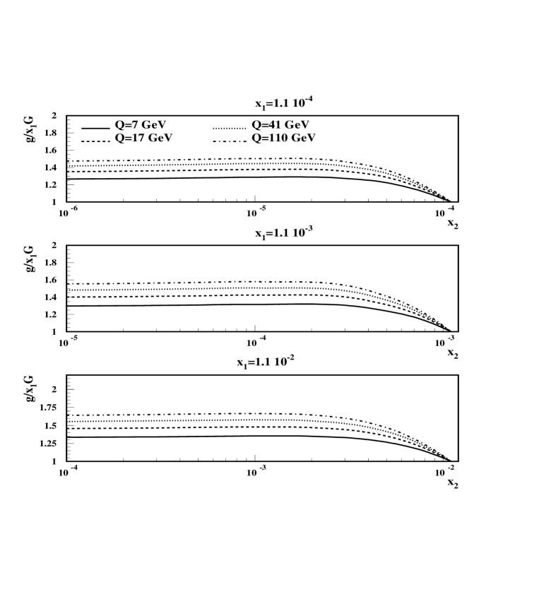
FIG. 1.: The fraction $g(x_{1},x_{2})/x_{1}G(x_{1})$ as a function of $x_{2}$ for fixed $x_{1}$ and various energies $Q$.

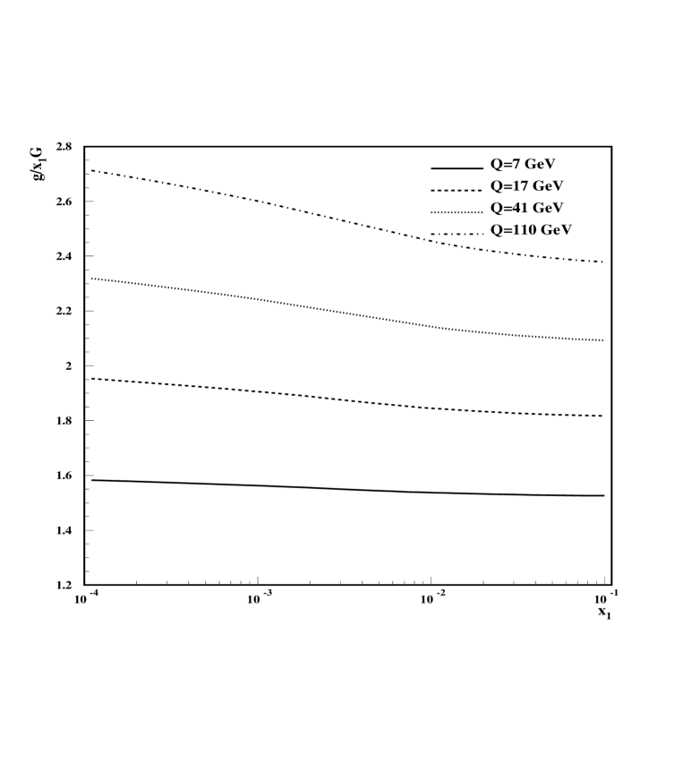
FIG. 2.: The fraction $g(x_{1},x_{2})/x_{1}G(x_{1})$ as a function of $x_{1}$ for $x_{2}=0$ and various energies $Q$.

REFERENCES

- [1] S.J. Brodsky, L.L. Frankfurt, J.F. Gunion, A.H. Mueller, and M. Strikman, Phys. Rev. D50 (1994) 3134; ibid. Erratum in print
- [2] L.L. Frankfurt, W. Koepf, and M. Strikman, Phys. Rev. D54 (1996) 3194.
- [3] A.Radyushkin Phys. Letters B385 (1996) 333.
- [4] J.C. Collins, L. Frankfurt, and M. Strikman, Phys. Rev. D56 (1997) 2982.
- [5] X.-D. Ji, Phys. Rev. D55 (1997) 7114.
- [6] A. Radyushkin, hep-ph/9704207, Phys. Rev D in press and private communications.
- [7] H. Abramowicz, L.L. Frankfurt and M. Strikman, DESY-95-047, SLAC Summer Inst. 1994:539-574.
- [8] J. Bartels and M.Loewe, Z.Phys. C12, 263 (1982).
- [9] Yu.L. Dokshitzer, D.I. Dyakonov and S.I. Troyan, Phys. Rep. Volume 58:270 (1980).
- [10] I.I Balitsky and V.M. Braun, Nucl. Phys. B311, 541 (1989).
- [11] L.V. Gribov, E.M. Levin and M.G. Ryskin, Phys. Rep., Vol. 100, (1983)
- [12] V.N. Gribov and L.N. Lipatov, Sov. J. Nucl. Phys., 15, 438 and 675 (1972).
- [13] V.N. Gribov, Lectures on the theory of complex momenta. KhFTI-70/48, Kharkov (1970).
- [14] J.C. Collins, D.E. Soper and G. Sterman, Factorization of Hard Processes in QCD, in “Perturabtive QCD” (A.H. Mueller, ed.) (World Scientific, Singapore, 1989).
- [15] J.C. Collins and G. Sterman, Nucl. Phys. B185, 172 (1981).
- [16] Yu.L. Dokshitzer, V.V. Khoze, A.H. Mueller and S.I. Troyan, “Basics of Perturbative QCD”, (Editions/Frontiers, 1991), pp.1-91.
- [17] A. Radyushkin, privat communications.
- [18] H.L. Lai et al. Phys. Rev. D55 (1997) 1280.
- [19] A. Freund and V. Guzey, preprint hep-ph/9801388