Abstract

Electroweak precision observables are calculated at complete 1-loop order in the extension of the standard model by an extra Higgs triplet, where the $\rho$-parameter can be different from unity already at the tree level. One additional data point is required for fixing the input parameters. In the on-shell renormalization scheme the leptonic mixing angle $\sin^{2}\theta_{e}$ at the $Z$ peak is chosen, together with the conventional input $\alpha,M_{Z},G_{\mu},m_{t}$. The calculated observables depend on the mass of the doublet Higgs boson $H^{0}$ and on the masses of the extra non-standard Higgs bosons as free parameters. The predictions of the standard model and the triplet model coincide for all observables in the experimental range of the top mass $m_{t}=175\pm 6$ GeV. In the triplet model, all observables which show a dependence on the doublet Higgs mass $M_{H^{0}}$ are consistent with a low value of $M_{H^{0}}$.

1 Introduction

In the light of the recent electroweak precision data the standard model with a single Higgs doublet is in a very good shape [1]. Whereas the data are compatible with a relatively light Higgs boson, direct empirical information on the scalar sector, however, is still lacking. A specific feature of the standard model assumption of a single Higgs field is the validity of the tree level relation

$$\rho\ =\ \frac{M_{W}^{2}}{M_{Z}^{2}\ \cos^{2}\theta_{W}}\ =\ 1$$

for the $\rho$-parameter, which measures the ratio between the neutral and charged current coupling strength [2]. $\rho$ deviates from unity by electroweak quantum effects, especially from the top-bottom doublet [3]. In more general scenarios, there are already tree level contributions to $\rho-1$, which however can only be of the order of the standard loop effects not to spoil the agreement with experimental data. A consistent formulation of such a scenario with $\rho_{tree}\neq 1$ requires the extension of the Higgs sector by at least an additional triplet of scalar fields with one extra vacuum expectation value different from zero. The full set of precision observables can be calculated, in analogy to the minimal model, in terms of a few input data points together with the standard loop contributions and the loops arising from the non-standard Higgs part. A complete discussion of the radiative corrections requires not only the evaluation of the extra loop diagrams with non-standard Higgs bosons, but also an extension of the renormalization procedure. Since $M_{W},M_{Z}$ and $\sin^{2}\theta_{W}$ are now independent parameters, one extra renormalization condition is necessary. This can be chosen in a formal way as done in the $\overline{MS}$-scheme [4], or in extension of the standard on-shell scheme [5] by choosing the electroweak mixing angle at the $Z$ peak, $\sin^{2}\theta_{e}$ for leptons, as an additional input parameter, together with the usual input $\alpha,G_{F},M_{Z}$.

In this paper we give a complete one-loop calculation of $M_{W}$ and the $Z$ boson observables in the simplest extension of the minimal model accommodating $\rho_{tree}\neq 1$. This model (discussed to some extent also in [6]) augments the standard model by an additional Higgs triplet with a VEV $\neq 0$ in the neutral sector. Besides the standard Higgs boson $H^{0}$ a further neutral scalar boson $K^{0}$ and a pair of charged Higgs particles $H^{\pm}$ form the physical spectrum. After specifying the model in section 2, we outline in section 3 the calculation in the aforementioned extended on-shell scheme. The predictions for the various observables and their parameter dependence are discussed and compared with the standard model predictions as well as with the experimental data in sections 4 and 5. Details of the calculation are collected in the appendix.

2 The standard model with an extra Higgs triplet

We consider the extension of the electroweak standard model where besides the ordinary Higgs doublet field

$$\Phi(x)=\left(\begin{array}[]{c}\phi^{+}(x)\\ \frac{1}{\sqrt{2}}(v+H^{0}(x)+i\chi(x))\end{array}\right)$$ (2.1)

an additional Higgs field $\Delta$ is introduced which transforms as a triplet under the symmetry group SU(2)$\times$U(1). Couplings of this extra field to fermions, although possible [7], are not considered for simplicity. The hypercharge is assigned as $Y_{\Delta}=0$, thus no particles with double electric charge occur. With a vacuum expectation value $u$ in the neutral component, the triplet can be written as [6]

$$\Delta=\left(\begin{array}[]{c}\Delta^{+}\\ \Delta^{0}=u+K^{0}\\ \Delta^{-}\end{array}\right)\;\quad\mbox{with}\quad{\Delta^{0}}^{*}=\Delta^{0}\,,\,{\Delta^{+}}^{*}=-\Delta^{-}\,.$$ (2.2)

Since there is no need for Higgs self couplings in our calculations, we can restrict our discussion to the extra Higgs term in the kinetic part of the Lagrangian

$${\cal L}_{\Delta-kin}=\frac{1}{2}(D_{\mu}\Delta)^{\dagger}(D^{\mu}\Delta).$$ (2.3)

The unphysical Higgs fields $G^{\pm},G_{Z}$ and the charged physical Higgs $H^{\pm}$ are linear combinations of the doublet and triplet field components

$$\left(\begin{array}[]{c}G^{\pm}\\ H^{\pm}\end{array}\right)=\left(\begin{array}[]{cc}\cos{\delta}&\pm\sin{\delta}\\ -\sin{\delta}&\pm\cos{\delta}\end{array}\right)\left(\begin{array}[]{c}\phi^{\pm}\\ \Delta^{\pm}\end{array}\right)\quad,\quad G_{Z}=\chi\quad,$$ (2.4)

where the mixing angle $\delta$ is determined by the vacuum expectation values $u$ and $v$:

$$\cos^{2}\!\delta=\frac{v^{2}}{v^{2}+4u^{2}}\,.$$ (2.5)

Besides the standard Higgs $H^{0}$, there is a further neutral physical Higgs field $K^{0}$. In the Feynman-’t Hooft gauge the unphysical fields $G^{\pm}$ and $G_{Z}$ get the same masses as the corresponding vector bosons. The masses of the remaining physical fields $H^{0},K^{0},H^{\pm}$ are free parameters.

In this model, in the following denoted as triplet model (TM), the masses of the $Z$ boson and the photon follow from $v$ as in the SM

$$M_{A}=0\quad,\quad M_{Z}=\frac{1}{2}\sqrt{g_{1}^{2}+g_{2}^{2}}\;v\quad,$$ (2.6)

but due to the additional vacuum expectation value $u$, the $W$-mass has changed to

$$M_{W}=\frac{1}{2}\,\frac{g_{2}v}{\cos\delta}\quad.$$ (2.7)

The electroweak mixing angle, which diagonalizes the neutral gauge boson mass matrix, is determined by

$$\cos{\theta_{W}^{Triplett}}=\frac{g_{2}}{\sqrt{g_{1}^{2}+g_{2}^{2}}}=:{c_{\theta}}\quad,\quad{s_{\theta}}^{2}=1-{c_{\theta}}^{2}\,.$$ (2.8)

It is related to the quantity (the mixing angle in the minimal model)

$$c_{W}=\frac{M_{W}}{M_{Z}}\quad,\quad s_{W}^{2}=1-c_{W}^{2}$$ (2.9)

in the following way:

$$c_{\theta}=c_{W}\cos\delta\quad.$$ (2.10)

This means that for $u\neq 0$, the $\rho$-parameter is different from unity already at the tree level:

$$\rho\,\equiv\,\frac{M_{W}^{2}}{M_{Z}^{2}c_{\theta}^{2}}=\frac{1}{\cos^{2}\delta}\quad.$$ (2.11)

3 One-loop calculations and renormalization

In order to obtain finite amplitudes in the TM at the 1-loop level we perform the renormalization in an on-shell scheme which is similar to the one described in [5] for the minimal SM. Compared to the minimal model, the TM has one more independent parameter in the gauge boson - fermion sector, which may be chosen as $\rho$ or ${s_{\theta}}^{2}$. For the renormalization procedure it is more convenient to treat ${s_{\theta}}^{2}$ as an additional independent input parameter and fix its counter term $\delta{s_{\theta}}^{2}$ by an appropriate renormalization condition. The other basic on-shell parameters with independent counter terms are $M_{W},M_{Z}$ and the electric charge $e$, which are renormalized by the same set of conditions as in the minimal model [5]. $\rho$ then appears as a derived quantity.

The renormalized vector boson self energies at the 1-loop level have the following counter term structure:

     =
     +
$\hat{\Sigma}^{\gamma\gamma}(k^{2})$
     = $\Sigma^{\gamma\gamma}(k^{2})$
     + $\delta Z_{2}^{\gamma}\,k^{2}$
$\hat{\Sigma}^{ZZ}(k^{2})$
     = $\Sigma^{ZZ}(k^{2})$
     + $\delta Z_{2}^{Z}(k^{2}-M_{Z}^{2})-\delta M_{Z}^{2}$
$\hat{\Sigma}^{WW}(k^{2})$
     = $\Sigma^{WW}(k^{2})$
     + $\delta Z_{2}^{W}(k^{2}-M_{W}^{2})-\delta M_{W}^{2}$
$\hat{\Sigma}^{\gamma Z}(k^{2})$
     = $\Sigma^{\gamma Z}(k^{2})$
     + $(\delta Z_{1}^{\gamma Z}-\delta Z_{2}^{\gamma Z})M_{Z}^{2}-\delta Z_{2}^{\gamma Z}\,k^{2}$

with

$$\delta Z_{i}^{\gamma Z}=\frac{c_{\theta}s_{\theta}}{c_{\theta}^{2}-s_{\theta}^{2}}(\delta Z_{i}^{Z}-\delta Z_{i}^{\gamma})\quad.$$ (3.1)

The $\Sigma^{\alpha\beta}$ denote the unrenormalized one-loop vector boson self energies of the TM (see appendix). The on-shell conditions determine the counter terms as follows:

$$\delta M_{W}^{2} = {\rm Re\,}\Sigma^{WW}(M_{W}^{2})$$

$$\delta M_{Z}^{2} = {\rm Re\,}\left[\Sigma^{ZZ}(M_{Z}^{2})-\frac{(\hat{\Sigma}^{\gamma Z}(M_{Z}^{2}))^{2}}{M_{Z}^{2}+\hat{\Sigma}^{\gamma\gamma}(M_{Z}^{2})}\right]$$

$$\delta Z_{1}^{\gamma} = -\Pi^{\gamma}(0)-\frac{s_{\theta}}{c_{\theta}}\,\frac{\Sigma^{\gamma Z}(0)}{M_{Z}^{2}}\quad\mbox{with}\quad\Pi^{\gamma}(0)=\frac{\partial\Sigma^{\gamma\gamma}}{\partial k^{2}}(0)$$

$$\delta Z_{2}^{\gamma} = -\Pi^{\gamma}(0)$$

$$\delta Z_{1}^{Z} = -\Pi^{\gamma}(0)-\frac{3c_{\theta}^{2}-2s_{\theta}^{2}}{s_{\theta}c_{\theta}}\,\frac{\Sigma^{\gamma Z}(0)}{M_{Z}^{2}}+\frac{c_{\theta}^{2}-s_{\theta}^{2}}{c_{\theta}^{2}}\,\frac{\delta s_{\theta}^{2}}{s_{\theta}^{2}}$$

$$\delta Z_{2}^{Z} = -\Pi^{\gamma}(0)-2\,\frac{c_{\theta}^{2}-s_{\theta}^{2}}{s_{\theta}c_{\theta}}\,\frac{\Sigma^{\gamma Z}(0)}{M_{Z}^{2}}+\frac{c_{\theta}^{2}-s_{\theta}^{2}}{c_{\theta}^{2}}\,\frac{\delta s_{\theta}^{2}}{s_{\theta}^{2}}\,$$

$$\delta Z_{1}^{W} = -\Pi^{\gamma}(0)-\frac{3-2s_{\theta}^{2}}{s_{\theta}c_{\theta}}\,\frac{\Sigma^{\gamma Z}(0)}{M_{Z}^{2}}+\frac{\delta s_{\theta}^{2}}{s_{\theta}^{2}}$$

$$\delta Z_{2}^{W} = -\Pi^{\gamma}(0)-2\,\frac{c_{\theta}}{s_{\theta}}\,\frac{\Sigma^{\gamma Z}(0)}{M_{Z}^{2}}+\frac{\delta s_{\theta}^{2}}{s_{\theta}^{2}}\quad.$$ (3.2)

Herein the additional constant $\delta s_{\theta}^{2}$ appears, which is formally related to the $Z$-factors by

$$\frac{\delta s_{\theta}^{2}}{s_{\theta}^{2}}=\frac{c_{\theta}}{s_{\theta}}\,(3\,\delta Z_{2}^{\gamma Z}-2\,\delta Z_{1}^{\gamma Z})\quad.$$ (3.3)

In the SM, the renormalization of the mixing angle in the on-shell scheme is not independent but related to the $W,Z$ mass renormalization according to

$$\frac{\delta s_{W}^{2}}{c_{W}^{2}}=\frac{\delta M_{Z}^{2}}{M_{Z}^{2}}-\frac{\delta M_{W}^{2}}{M_{W}^{2}}\quad.$$ (3.4)

Here, in the TM, $\delta{s_{\theta}}^{2}$ has to be fixed by an extra renormalization condition. We do this by the identification of ${s_{\theta}}$ with the effective leptonic mixing angle $\sin\!\theta^{\rm lep}_{\rm eff}$ at the $Z$ resonance

$${s_{\theta}}^{2}\,=\,\sin^{2}\!\theta_{\rm eff}^{\rm lep}$$ (3.5)

which determines the ratio of the leptonic effective vector and axial vector coupling constants of the $Z^{0}$ in the following way:

$$\frac{{\rm Re\,}(g_{V}^{e})}{{\rm Re\,}(g_{A}^{e})}=1-4s_{\theta}^{2}\,.$$ (3.6)

This is an implicit equation for $\delta{s_{\theta}}^{2}$ which enters ratio of the coupling constants (see equations (4.7)) at 1-loop through the counter term to the vector form factor of the $Zee$ weak vertex correction. Its explicit form is given below in eq. (3.10).

The renormalized vector boson fermion vertices $\hat{\Gamma}$ are expressed in terms of the unrenormalized vertices $\Gamma$ and the corresponding counter terms as follows:

     =
     +
$\hat{\Gamma}_{\mu}^{Zff}$
     = $\Gamma_{\mu}^{Zff}$
     + $i\frac{\textstyle e}{\textstyle 2s_{\theta}c_{\theta}}\;\gamma_{\mu}\;C_{V}^{Zff}-i\frac{\textstyle e}{\textstyle 2s_{\theta}c_{\theta}}\;\gamma_{\mu}\gamma_{5}\;C_{A}^{Zff}$
$\hat{\Gamma}_{\mu}^{W\tilde{f}f}$
     = $\Gamma_{\mu}^{W\tilde{f}f}$
     + $i\frac{\textstyle e}{\textstyle 2\sqrt{2}{s_{\theta}}}\;\gamma_{\mu}(1-\gamma_{5})\;C_{L}^{W\tilde{f}f}$

$$\mbox{with}\quad C_{V}^{Zff} = v_{f}(\delta Z_{1}^{Z}-\delta Z_{2}^{Z})+2s_{\theta}c_{\theta}Q_{f}(\delta Z_{1}^{\gamma Z}-\delta Z_{2}^{\gamma Z})$$

$$+(v_{f}\delta Z_{V}^{f}+a_{f}\delta Z_{A}^{f})$$

$$C_{A}^{Zff} = a_{f}(\delta Z_{1}^{Z}-\delta Z_{2}^{Z})+(v_{f}\delta Z_{A}^{f}+a_{f}\delta Z_{V}^{f})$$

$$C_{L}^{W\tilde{f}f} = \delta Z_{1}^{W}-\delta Z_{2}^{W}+\delta Z_{L}$$

$$\mbox{and}\quad v_{f} = I_{3}^{f}-2s_{\theta}^{2}Q_{f}\quad,\quad a_{f}=I_{3}^{f}\quad.$$ (3.7)

The fermion wave function renormalization constants $\delta Z_{V,A}$, and $\delta Z_{L}$ resp., follow in the usual way from the “residue = 1” condition for the fermions attached to the vertex (see appendix, eq. (A.10) ).

Neglecting the small terms proportional to the fermion masses $m_{f}$, the $Z$ vertices have only vector and axial vector contributions: $\hat{\Lambda}_{A,V}^{Zff}$ is the renormalized vector or axial-vector correction, as it appears in the decomposition of the $Zff$ vertex function

$$\hat{\Gamma}_{\mu}^{Zff}=i\,\frac{e}{2{s_{\theta}}{c_{\theta}}}\,\left[\gamma_{\mu}(v_{f}-a_{f}\gamma_{5})+\gamma_{\mu}\hat{\Lambda}_{V}^{Zff}+\gamma_{\mu}\gamma_{5}\hat{\Lambda}_{A}^{Zff}\right]\quad.$$ (3.8)

Using the formulas for the effective $Z$ couplings (4.7), the renormalization condition for ${s_{\theta}}^{2}$, eq. (3.6), can be written as follows:

$${\rm Re\,}\left\{-\frac{\hat{\Pi}^{\gamma Z}(M_{Z}^{2})}{v_{e}}+\frac{1}{2{s_{\theta}}{c_{\theta}}}\left(\frac{\hat{\Lambda}_{V}^{Zee}(M_{Z}^{2})}{v_{e}}-\frac{\hat{\Lambda}_{A}^{Zee}(M_{Z}^{2})}{a_{e}}\right)\right\}=0\quad,$$ (3.9)

which can be solved for $\delta{s_{\theta}}^{2}$ yielding

$$\frac{\delta{s_{\theta}}^{2}}{{s_{\theta}}^{2}}={\rm Re\,}\left\{\frac{{c_{\theta}}}{{s_{\theta}}}\left[\frac{v_{e}^{2}-a_{e}^{2}}{a_{e}}\Sigma_{A}^{e}(m_{e}^{2})+\frac{\Sigma^{\gamma Z}(M_{Z}^{2})}{M_{Z}^{2}}-\frac{v_{e}}{2{s_{\theta}}{c_{\theta}}}\left(\frac{\Lambda_{V}^{Zee}(M_{Z}^{2})}{v_{e}}-\frac{\Lambda_{A}^{Zee}(M_{Z}^{2})}{a_{e}}\right)\right]\right\}\quad.$$ (3.10)

Therein, $\Lambda_{V,A}^{Zee}$ are the vector and axial vector form factors of the unrenormalized 1-loop $Zee$ vertex correction in the normalization of eq. (3.8), and $\Sigma_{A}^{e}$ is the axial part of the $e$ self energy.

In contrast to the mixing angle counter term in the minimal model, there is no quadratic $m_{t}$-dependence in $\delta{s_{\theta}}^{2}$. The top mass enters via $\Sigma^{\gamma Z}$, where the dependence is only logarithmic.

4 Radiative corrections for precision observables

In order to fix the free parameters of the model we choose as precise input quantities as usual the electromagnetic fine structure constant $\alpha$ (together with the fermionic vacuum polarization at the $M_{Z}$ scale), the Fermi constant $G_{\mu}$, and the $Z$ mass $M_{Z}$, together with the experimental value of ${s_{\theta}}^{2}$ as the fourth input parameter for the TM. The parameters appearing in 1-loop order are the top mass and the masses $M_{H^{0}},M_{K^{0}},M_{H^{\pm}}$ of the standard and non-standard Higgs bosons. The $W$ mass $M_{W}$ and the $Z$ resonance parameters then follow as predictions and can be compared with the experimental results.

4.1 Muon decay width and $M_{W}$

The muon decay width reads in the Fermi model

$$\Gamma_{\mu}^{F}=\frac{G_{\mu}^{2}m_{\mu}^{5}}{192\,\pi^{3}}\left(1-\frac{8m_{e}^{2}}{m_{\mu}^{2}}\right)\cdot C^{Fermi}_{QED}\quad.$$ (4.1)

In the TM it is given by the expression (see also [8])

$$\Gamma_{\mu}=\;\frac{\alpha^{2}}{384\,\pi}\;\frac{m_{\mu}^{5}}{M_{W}^{4}s_{\theta}^{4}}\;\left(1-\frac{8m_{e}^{2}}{m_{\mu}^{2}}\right)\cdot\left(\frac{1}{1-\Delta\tilde{r}}\right)^{2}\cdot C^{Fermi}_{QED}$$ (4.2)

with $$\Delta\tilde{r}=\frac{\hat{\Sigma}^{WW}(0)}{M_{W}^{2}}+\frac{\alpha}{4\pi s_{\theta}^{2}}\left(6+\frac{10-10s_{\theta}^{2}-3\,(\frac{R}{c_{\theta}^{2}})\,(1-2s_{\theta}^{2})}{2(1-R)}\,\ln R\right)$$ (4.3)

and $$R=\frac{M_{W}^{2}}{M_{Z}^{2}}\quad.$$ (4.4)

The QED correction factor $C^{Fermi}_{QED}$ [9] is the same in both models. The relation between the $W$ mass and the basic input quantities is thus given by

$$M_{W}^{2} = \rho\,M_{Z}^{2}(1-s_{\theta}^{2})$$ (4.5)

$$\rho = \frac{A}{M_{Z}^{2}(1-\Delta\tilde{r})\,s_{\theta}^{2}(1-s_{\theta}^{2})}$$ (4.6)

with $$A=\frac{\alpha\pi}{\sqrt{2}G_{\mu}}\quad.$$

Through $\Delta\tilde{r}(M_{Z},M_{W},{s_{\theta}};m_{t},M_{H^{0}},M_{K^{0}},M_{H^{\pm}})$ the relations (4.5) and (4.6) are implicit equations, which can be solved iteratively for $M_{W}$ and $\rho$.

4.2 Effective $Zff$ couplings and $Z$ resonance observables

Having determined $\rho$ and $\Delta\tilde{r}$ with the help of $G_{\mu}$ in the way described above, the effective couplings of the $Z$-boson to fermions $f\neq t$ can be written in the following way:

$$g_{V}^{f} = \left(\rho\,\frac{1-\Delta\tilde{r}}{1+\hat{\Pi}^{Z}(M_{Z}^{2})}\right)^{\frac{1}{2}}\cdot\left[v_{f}+2{s_{\theta}}{c_{\theta}}Q_{f}\hat{\Pi}^{\gamma Z}(M_{Z}^{2})+F_{V}^{Zf}(M_{Z}^{2})\right]$$

$$g_{A}^{f} = \left(\rho\,\frac{1-\Delta\tilde{r}}{1+\hat{\Pi}^{Z}(M_{Z}^{2})}\right)^{\frac{1}{2}}\cdot\left[a_{f}+F_{A}^{Zf}(M_{Z}^{2})\right]\quad.$$ (4.7)

The equations (4.7) include besides the renormalized vertex form factors $F_{V,A}^{Zf}=\hat{\Lambda}_{V,A}^{Zff}$ the correction to the $Z$ propagator

$$\hat{\Pi}^{Z}(M_{Z}^{2}) = \left.{\rm Re\,}\frac{d\hat{\Sigma}^{Z}(s)}{ds}\right|_{s=M_{Z}^{2}}$$ (4.8)

with

$$\hat{\Sigma}^{Z}(s)\,=\,\hat{\Sigma}^{ZZ}(s)-\frac{(\hat{\Sigma}^{\gamma Z}(s))^{2}}{s+\hat{\Sigma}^{\gamma\gamma}(s)}\,,$$

and the photon-$Z$ mixing

$$\hat{\Pi}^{\gamma Z}(M_{Z}^{2})=\frac{\hat{\Sigma}^{\gamma Z}(M_{Z}^{2})}{M_{Z}^{2}+\hat{\Sigma}^{\gamma\gamma}(M_{Z}^{2})}\quad.$$ (4.9)

The self energies are from section 2.

The effective coupling constants (real parts only) determine the on-resonance asymmetries via the combinations

$$A_{f}=\frac{2g_{V}^{f}g_{A}^{f}}{(g_{V}^{f})^{2}+(g_{A}^{f})^{2}}\,.$$ (4.10)

In particular:
$-$ the forward backward asymmetries

$$A_{FB}^{f}=\frac{3}{4}A_{e}\cdot A_{f}$$ (4.11)

$-$ the left-right asymmetry

$$A_{LR}=A_{e}$$ (4.12)

$-$ the $\tau$ polarization

$$P_{\tau}=A_{\tau}\,.$$ (4.13)

The fermionic partial widths, expressed in terms of the effective coupling constants read up to 2nd order in the fermion masses:

$$\Gamma_{f} = \Gamma_{0}\,\left((g_{V}^{f})^{2}+(g_{A}^{f})^{2}(1-\frac{6m_{f}^{2}}{M_{Z}^{2}})\right)\cdot(1+Q_{f}^{2}\,\frac{3\alpha}{4\pi})+\Delta\Gamma^{f}_{QCD}$$ (4.14)

with

$$\Gamma_{0}\,=\,N_{C}^{f}\,\frac{\sqrt{2}G_{\mu}M_{Z}^{3}}{12\pi},\;\;\;\;N_{C}^{f}=1\mbox{ (leptons)},\;\;=3\mbox{ (quarks)}.$$

and the QCD corrections $\Delta\Gamma^{f}_{QCD}$ for quark final states. The QCD correction for the light quarks with $m_{q}\simeq 0$ is given by

$$\Delta\Gamma^{f}_{QCD}\,=\,\Gamma_{0}\left((g_{V}^{f})^{2}+(g_{A}^{f})^{2}\right)\cdot K_{QCD}$$ (4.15)

with [10]

$$K_{QCD}=\frac{\alpha_{s}}{\pi}+1.41\left(\frac{\alpha_{s}}{\pi}\right)^{2}-12.8\left(\frac{\alpha_{s}}{\pi}\right)^{3}-\frac{Q_{f}^{2}}{4}\frac{\alpha\alpha_{s}}{\pi^{2}}\,.$$

For $b$ quarks the QCD corrections are different due to finite $b$ mass terms and to top quark dependent 2-loop diagrams for the axial part:

$$\Delta\Gamma_{QCD}^{b}=\Delta\Gamma_{QCD}^{d}\,+\,\Gamma_{0}\left[(g_{V}^{b})^{2}\,R_{V}\,+\,(g_{A}^{b})^{2}\,R_{A}\right]\,.$$

For the coefficients $R_{V,A}$ see e.g. [11].

5 Results and discussion

Besides the standard input data points $G_{\mu}=1.16639\cdot 10^{-5}\;{\rm GeV}^{-2}$ [12], $\alpha(M_{Z})=1/128.89\pm 0.09$ [13] and $M_{Z}=91.1863\pm 0.0020\;{\rm GeV}$ [1], we use the effective mixing angle ${s_{\theta}}^{2}=0.23165\pm 0.00024$ at $M_{Z}$ as given in [1]. Besides $m_{t}$, the predictions in the TM depend on the masses of the various Higgs bosons. In general, the dependence on the Higgs masses is very smooth. In order to visualize the different dependence of the predictions on the top mass in the various models, we display the results over a large top mass range and indicate the experimental data.

5.1 The $W$ mass and the $\rho$ parameter

In Figure 5.1 the top mass dependence of $M_{W}$ is displayed for a set of masses for the doublet Higgs boson $H^{0}$, both in the minimal model (SM) and the standard model with the extra triplet (TM). The other Higgs masses have been fixed at 300 GeV. The dependence on both $m_{t}$ and $M_{H^{0}}$ is weaker in the TM compared to the SM. The experimental result

$$M_{W}=80.356\pm 0.125\;\mbox{GeV}\quad\cite[cite]{[\@@bibref{}{Blondel:96}{}{}]}\quad,\quad m_{t}=175\pm 6\;\mbox{GeV}\quad\cite[cite]{[\@@bibref{}{Tipton:96}{}{}]}$$

is shown as the data point with error bars. It is placed right in the cross-over region of the two models.

Figure 5.1: Top mass dependence of $M_{W}$ in the SM and the TM for various doublet Higgs masses $M_{H^{0}}$. The input values for the TM Higgs masses $M_{K^{0}}$ and $M_{H^{\pm}}$ are 300 GeV.

In the TM, $M_{W}$ has a strong dependence on the value of the input parameter ${s_{\theta}}^{2}$. This is illustrated in Fig. 5.2 for different values of the charged Higgs mass, with both the neutral Higgs masses at 300 GeV. Compared with the experimental data, the sensitivity to $M_{H^{\pm}}$ is not very striking. Higher masses are slightly prefered, in particular for a low value of ${s_{\theta}}^{2}$. The variation with $m_{t}$ in its experimental $1\sigma$ range is hardly visible.

Figure 5.2: Dependence of $M_{W}$ on the input parameter ${s_{\theta}}^{2}$ for various values of $m_{t}$ and $M_{H^{\pm}}$ in the TM. The masses for the neutral Higgs bosons are fixed at 300 GeV.

An interesting quantity is the $\rho$-parameter, eq. (2.11) which can act as an indicator for a deviating Higgs structure. Since also in the SM $\rho$ is different from unity by radiative corrections, a sensible comparison of different models is only possible at the 1-loop order. The experimental value derived from $M_{W}$, $M_{Z}$ and $\sin^{2}\!\theta_{\rm eff}^{\rm lep}$ [1] is given by

$$\rho=1.0107\pm 0.0032.$$ (5.1)

The dependence of $\rho$ on the model parameters is shown in Fig. 5.3 and Fig. 5.4 for SM and TM, together with the experimental data. The models overlap in the region of the data, which is equivalent to the situation in the corresponding figure with $M_{W}$.

Figure 5.3: Top mass dependence of the $\rho$ parameter in the SM and the TM for various doublet Higgs masses $M_{H^{0}}$. The input values for the TM Higgs masses $M_{K^{0}}$ and $M_{H^{\pm}}$ are 300 GeV.

Figure 5.4: Dependence of the $\rho$ parameter on the input parameter ${s_{\theta}}^{2}$ in the TM for various values of $m_{t}$ and $M_{H^{\pm}}$. The masses of the neutral Higgs bosons are fixed at 300 GeV.

5.2 $Z$ boson observables

Precision observables at the $Z$ resonance are the total and partial $Z$ decay widths and the peak asymmetries. The total $Z$ width can be expressed as the sum of the fermionic partial widths

$$\Gamma_{Z}=\sum_{f}\Gamma_{f}\quad,$$ (5.2)

which are defined in equation (4.14).

Similar to $M_{W}$, we display the total width $\Gamma_{Z}$ in Fig. 5.5 versus $m_{t}$ for the SM and the TM, together with the experimental data point $\Gamma_{Z}=2.4946\pm 0.0027\;{\rm GeV}$ [1]. Although the models show a different behaviour with $m_{t}$ and $M_{H}$, they coincide in the region where both models agree with the data. It is interesting to note that the SM has a preference for a heavy Higgs from the observable $\Gamma_{Z}$, whereas the mixing angle measurement requires a light Higgs boson. In the TM, a light $H^{0}$ is compatible with all precision observables. Fig. 5.6 makes the TM correlation between ${s_{\theta}}^{2}$ and $M_{H^{0}}$ in the $Z$ width more explicit for the measured value of the top mass.

Figure 5.5: Top mass dependence of the total $Z$ width in the SM and the TM for various doublet Higgs masses $M_{H^{0}}$. The input values for the TM Higgs masses $M_{K^{0}}$ and $M_{H^{\pm}}$ are 300 GeV.

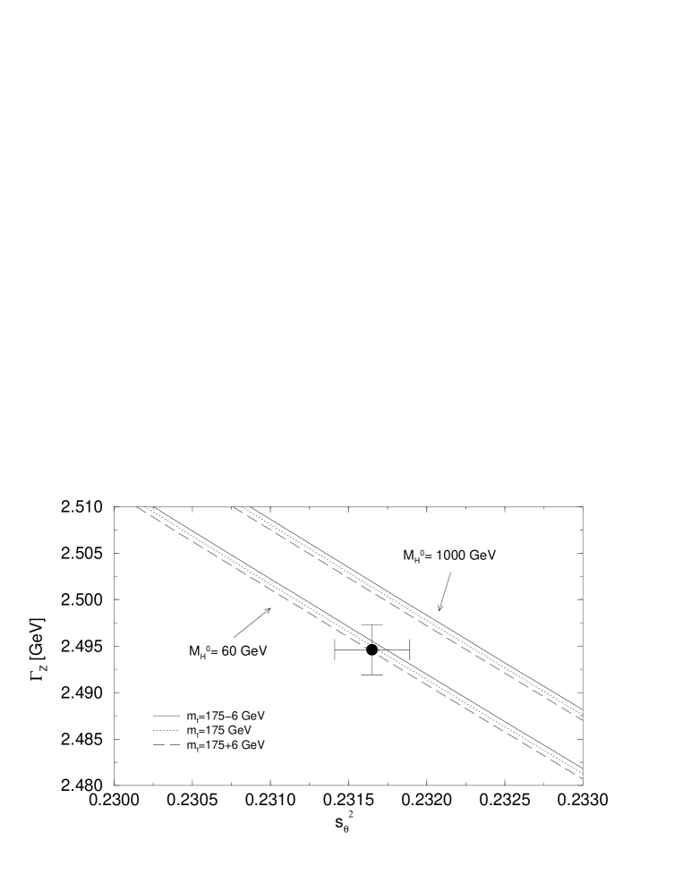
Figure 5.6: Dependence of the total $Z$ width on the input parameter ${s_{\theta}}^{2}$ for various values of $m_{t}$ and $M_{H^{0}}$. The masses of the triplet Higgs bosons are fixed at 300 GeV.

Partial widths are conveniently discussed in terms of the ratios

$$R_{Z}=\frac{\Gamma_{\rm had}}{\Gamma_{e}}\quad,\quad R_{c}=\frac{\Gamma_{c}}{\Gamma_{\rm had}}\quad\mbox{and}\quad R_{b}=\frac{\Gamma_{b}}{\Gamma_{\rm had}}\quad,$$ (5.3)

which are experimentally determined to [1]

$$R_{Z} = 20.778\pm 0.029$$

$$R_{c} = 0.1715\pm 0.0056$$

$$R_{b} = 0.2178\pm 0.0011\quad.$$

The predictions for $R_{Z}$ by the SM and the TM are illustrated in Fig. 5.7. In contrast to the previously discussed observables, the $m_{t}$-dependence of $R_{Z}$ is stronger in the TM. $R_{Z}$ is, however, completely insensitive to any Higgs mass. Again we encounter the situation that the two models coincide exactly in that range where the experimental data are placed.

The quantity $R_{c}$ is not very instructive with respect to the Higgs sector. Fig. 5.8 contains the predictions for $R_{c}$, which in view of the comparatively large experimental error can be considered as identical and in best agreement with the data.

An observable of special interest is the quantity $R_{b}$ with its experimental value about $1.8\,\sigma$ above the SM prediction. Its special sensitivity to $m_{t}$ is based on the virtual presence of the top quark in the $Z\bar{b}b$ vertex corrections. Fig. 5.9 shows the predictions of both the SM and TM, which with exception of very high top masses are the same, with practically no Higgs dependence. The deviation from the data point hence is also the same in both type of models.

The leptonic on-resonance asymmetries are in the TM completely determined by the value of the input parameter ${s_{\theta}}^{2}$, which is the leptonic mixing angle (and actually determined from asymmetry measurements). For the purpose of illustration, we present in Fig. 5.10 the left-right asymmetry $A_{LR}$ as predicted by the SM in terms of $m_{t}$ and $M_{H}$, and the range corresponding to the TM input ${s_{\theta}}^{2}=0.023165\pm 0.00024$. This range, indicated by the shaded area, can be identified with the TM “prediction”. The SM requires a light Higgs boson, which is disfavoured by the total width $\Gamma_{Z}$ (Fig. 5.5), in contrast to the TM. The experimental value as measured by the SLD collaboration is given by [1]

$$A_{LR}=0.1542\pm 0.0037\quad.$$ (5.4)

The hadronic forward-backward asymmetries for $c$ and $b$ quark final states contain besides $A_{e}$ the additional factors $A_{c,b}$ in eq. (4.11). In practice, however, the model dependence beyond ${s_{\theta}}^{2}$ cancels in the ratios. Consequently, the TM predictions in Fig. 5.11 and Fig. 5.12 appear as a top and Higgs mass independent horizontal line for each fixed value of ${s_{\theta}}^{2}$. Varying ${s_{\theta}}^{2}$ in the $1\,\sigma$ range yields the shaded band. The SM predictions, on the other hand, do depend on $m_{t}$ and $M_{H}$, essentially through ${s_{\theta}}^{2}$. The experimental results are given by [1]

$$A_{FB}^{c}=0.07351\pm 0.00484\quad\mbox{and}\quad A_{FB}^{b}=0.09790\pm 0.00231\quad.$$ (5.5)

Figure 5.7: Top mass dependence of $R_{Z}$ in the SM and the TM for various Higgs masses.

Figure 5.8: Top mass dependence of $R_{c}$ in the SM and the TM for various Higgs masses. The error bar of $R_{c}$ covers the full vertical axis.

Figure 5.9: Top mass dependence of $R_{b}$ in the SM and the TM for various Higgs masses.

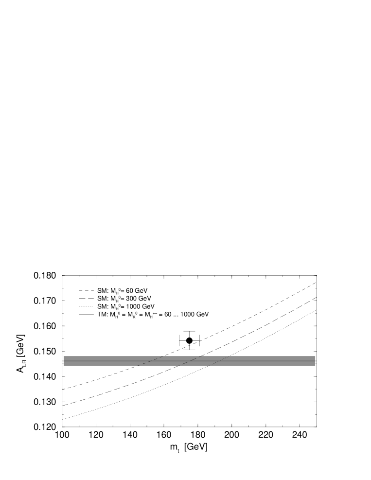
Figure 5.10: Left/Right asymmetry in the SM and the TM. The shaded area corresponds to a variation of ${s_{\theta}}^{2}=0.23165\pm 0.00024$.

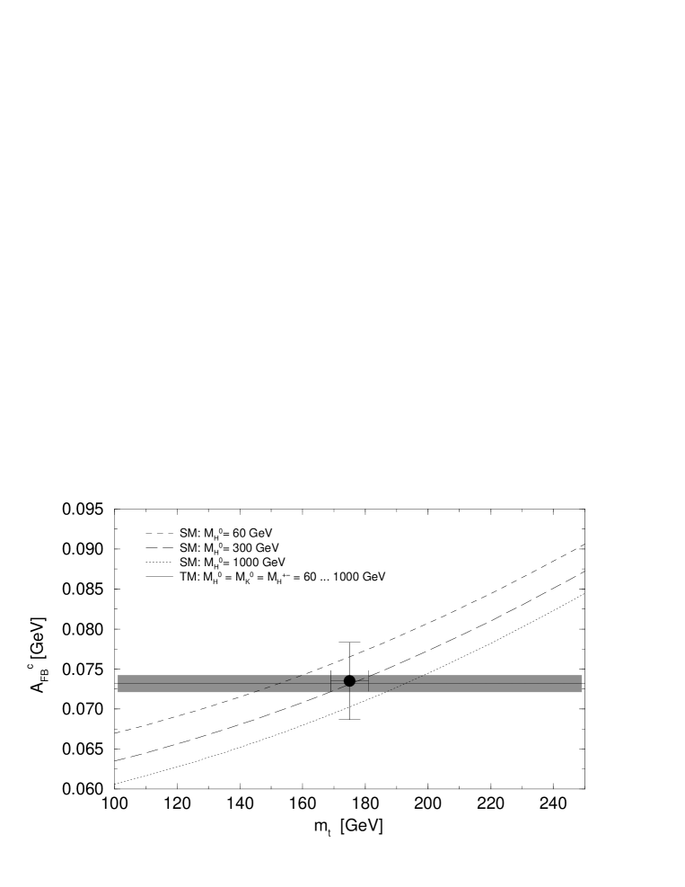
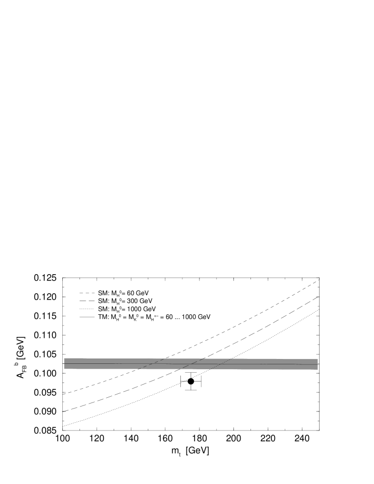
Figure 5.11: Forward/backward asymmetry for charm quarks in the SM and the TM. The shaded area corresponds to a variation of ${s_{\theta}}^{2}=0.23165\pm 0.00024$.

Figure 5.12: Forward/backward asymmetry for bottom quarks in the SM and the TM. The shaded area corresponds to a variation of ${s_{\theta}}^{2}=0.23165\pm 0.00024$.

Whereas $A_{FB}^{c}$ is perfect for both models, $A_{FB}^{b}$ needs a large Higgs mass in the SM, opposite to the requirement from $A_{LR}$. The TM coincides with the SM in the intermediate range of $M_{H^{0}}$; it is also slightly higher than the experimental value.

6 Conclusions

We have presented a complete 1-loop calculation of electroweak precision observables in the extension of the SM by an extra Higgs triplet, where the $\rho$-parameter can be different from unity already at the tree level. Since the gauge - fermion sector has one free parameter more compared to the SM, one additional data point is required for fixing the input parameters. Choosing the effective leptonic mixing angle, the observables depend, besides on ${s_{\theta}}^{2}$ and the conventional input $\alpha,M_{Z},G_{\mu},m_{t}$, on the mass of the doublet Higgs boson $H^{0}$ and on the masses of the extra non-standard Higgs bosons as free parameters. The predictions of the SM and the TM coincide for all observables in the experimental range of the top mass $m_{t}=175\pm 6$ GeV. In this range, both models fully agree with the experimental precision data, with two exceptions: $R_{b}$, $A^{b}_{FB}$, where both models show similar deviations from the data. The two types of models are thus indistinguishable, and no signal for a non-standard Higgs structure can be found in the data. In the TM all observables which show a dependence on the doublet Higgs mass, are consistent with a low value of $M_{H^{0}}$, whereas in the SM some observables like $\Gamma_{Z}$ advocate a large value for $M_{H^{0}}$.

Appendix

This section contains the analytic expressions for the vector boson and fermion self energies and the $Z\bar{f}f$ vertex corrections with internal Higgs states. Only those contributions are listed which are different from the minimal standard model. $\tilde{f}$ always denotes the isospin partner of the fermion $f$. Moreover, the following abbreviations are used:

$$c_{\delta}=\cos\delta\quad,\quad s_{\delta}=\sin\delta\quad.$$ (A.1)

The scalar 1-, 2- and 3-point functions in dimensional regularization are given by

$$\frac{i}{16\pi^{2}}\,A = \mu^{4-D}\int\frac{d^{D}k}{(2\pi)^{D}}\;\frac{1}{k^{2}-m^{2}}$$

$$\frac{i}{16\pi^{2}}\,B_{0} = \mu^{4-D}\int\frac{d^{D}k}{(2\pi)^{D}}\;\frac{1}{[k^{2}-m_{1}^{2}][(k+p)^{2}-m_{2}^{2}]}$$

$$\frac{i}{16\pi^{2}}\,C_{0} = \mu^{4-D}\int\frac{d^{D}k}{(2\pi)^{D}}\;\frac{1}{[k^{2}-m_{1}^{2}][(k+p_{1})^{2}-m_{2}^{2}][(k+p_{1}+p_{2})^{2}-m_{3}^{2}]}\quad,$$ (A.2)

We also need the scalar coefficients in the tensor integral decompositions [15]

$$B^{\mu} = p^{\mu}\>B_{1}(p^{2},m_{1},m_{2})$$

$$B^{\mu\nu} = g^{\mu\nu}B_{22}(p^{2},m_{1},m_{2})+p^{\mu}\,p^{\nu}\>B_{21}(p^{2},m_{1},m_{2})$$

$$C^{\mu} = p_{1}^{\mu}\>C_{11}+p_{2}^{\mu}\>C_{12}$$

$$C^{\mu\nu} = g^{\mu\nu}C_{20}+p_{1}^{\mu}\,p_{1}^{\nu}\>C_{21}+p_{2}^{\mu}\,p_{2}^{\nu}\>C_{22}+(p_{1}^{\mu}\,p_{2}^{\nu}+p_{1}^{\nu}\,p_{2}^{\mu})\>C_{23}\quad.$$ (A.3)

For the 2-point functions they are given by

$$B_{1}(p^{2},m_{1},m_{2}) = \frac{1}{2p^{2}}\left[A(m_{1})-A(m_{2})+(m_{2}^{2}-m_{1}^{2}-p^{2})B_{0}(p^{2},m_{1},m_{2})\right]$$

$$B_{22}(p^{2},m_{1},m_{2}) = \frac{1}{6}\left[A(m_{2})+2m_{1}^{2}B_{0}(p^{2},m_{1},m_{2})\right.$$

$$\left.+(p^{2}+m_{1}^{2}-m_{2}^{2})B_{1}(p^{2},m_{1},m_{2})+m_{1}^{2}+m_{2}^{2}-\frac{p^{2}}{3}\right]$$

$$B_{21}(p^{2},m_{1},m_{2}) = \frac{1}{3p^{2}}\left[A(m_{2})-m_{1}^{2}B_{0}(p^{2},m_{1},m_{2})\right.$$ (A.4)

$$\left.-2(p^{2}+m_{1}^{2}-m_{2}^{2})B_{1}(p^{2},m_{1},m_{2})-\frac{m_{1}^{2}+m_{2}^{2}}{2}+\frac{p^{2}}{6}\right]\quad.$$

For the corresponding expressions in the 3-point functions see e.g. [16].

Vector boson self energies:

For the vector boson self energies three diagram topologies with internal Higgs lines contribute. The analytic expressions given below correspond to the sum over all possibilities for $S$.

$$\Sigma^{\gamma\gamma}_{(SS)} = \frac{\alpha}{4\pi}\left\{-4B_{22}(k^{2},M_{H^{\pm}},M_{H^{\pm}})-4B_{22}(k^{2},M_{W},M_{W})\right\}$$

$$\Sigma^{ZZ}_{(SS)} = \frac{\alpha}{4\pi}\left(-\frac{1}{{s_{\theta}}^{2}{c_{\theta}}^{2}}\right)\left\{B_{22}(k^{2},M_{H^{0}},M_{Z})+(c_{\delta}^{2}+c_{\theta}^{2}-s_{\theta}^{2})^{2}B_{22}(k^{2},M_{H^{\pm}},M_{H^{\pm}})\right.$$

$$\left.+(s_{\delta}^{2}+c_{\theta}^{2}-s_{\theta}^{2})^{2}B_{22}(k^{2},M_{W},M_{W})+2s_{\delta}^{2}c_{\delta}^{2}B_{22}(k^{2},M_{H^{\pm}},M_{W})\right\}$$

$$\Sigma^{\gamma Z}_{(SS)} = \frac{\alpha}{4\pi}\frac{1}{{s_{\theta}}{c_{\theta}}}\left\{2({c_{\delta}}^{2}-{s_{\theta}}^{2}+{c_{\theta}}^{2})B_{22}(k^{2},M_{H^{\pm}},M_{H^{\pm}})\right.$$

$$\left.+2({s_{\delta}}^{2}-{s_{\theta}}^{2}+{c_{\theta}}^{2})B_{22}(k^{2},M_{W},M_{W})\right\}$$

$$\Sigma^{WW}_{(SS)} = \frac{\alpha}{4\pi}\left(-\frac{1}{{s_{\theta}}^{2}}\right)\left\{{s_{\delta}}^{2}B_{22}(k^{2},M_{H^{0}},M_{H^{\pm}})+{c_{\delta}}^{2}B_{22}(k^{2},M_{H^{0}},M_{W})\right.$$

$$\left.+4{c_{\delta}}^{2}B_{22}(k^{2},M_{K^{0}},M_{H^{\pm}})+4{s_{\delta}}^{2}B_{22}(k^{2},M_{K^{0}},M_{W})\right.$$

$$\left.+{s_{\delta}}^{2}B_{22}(k^{2},M_{Z},M_{H^{\pm}})+{c_{\delta}}^{2}B_{22}(k^{2},M_{Z},M_{W})\right\}$$

$$\Sigma^{\gamma\gamma}_{(S)} = \frac{\alpha}{4\pi}\left\{2A(M_{H^{\pm}})+2A(M_{W})\right\}$$

$$\Sigma^{ZZ}_{(S)} = \frac{\alpha}{4\pi}\frac{1}{4{s_{\theta}}^{2}{c_{\theta}}^{2}}\left\{A(M_{H^{0}})+A(M_{Z})+2(({c_{\theta}}^{2}-{s_{\theta}}^{2}+{c_{\delta}}^{2})^{2}+{s_{\delta}}^{2}{c_{\delta}}^{2})A(M_{H^{\pm}})\right.$$

$$\left.+2(({c_{\theta}}^{2}-{s_{\theta}}^{2}+{s_{\delta}}^{2})^{2}+{s_{\delta}}^{2}{c_{\delta}}^{2})A(M_{W})\right\}$$

$$\Sigma^{\gamma Z}_{(S)} = \frac{\alpha}{4\pi}\frac{1}{{s_{\theta}}{c_{\theta}}}\left\{({s_{\theta}}^{2}-{c_{\theta}}^{2}-{c_{\delta}}^{2})A(M_{H^{\pm}})+({s_{\theta}}^{2}-{c_{\theta}}^{2}-{s_{\delta}}^{2})A(M_{W})\right\}$$

$$\Sigma^{WW}_{(S)} = \frac{\alpha}{4\pi}\frac{1}{4{s_{\theta}}^{2}}\left\{A(M_{H^{0}})+4A(M_{K^{0}})+A(M_{Z})+2(1+{c_{\delta}}^{2})A(M_{H^{\pm}})\right.$$

$$\left.+2(1+{s_{\delta}}^{2})A(M_{W})\right\}$$

$$\Sigma^{\gamma\gamma}_{(VS)} = \frac{\alpha}{4\pi}2M_{W}^{2}B_{0}(k^{2},M_{W},M_{W})$$

$$\Sigma^{ZZ}_{(VS)} = \frac{\alpha}{4\pi}\frac{M_{Z}^{2}}{{s_{\theta}}^{2}}\left\{\frac{1}{{c_{\theta}}^{2}}B_{0}(k^{2},M_{H^{0}},M_{Z})+2{s_{\delta}}^{2}B_{0}(k^{2},M_{H^{\pm}},M_{W})\right.$$

$$\left.+2\frac{({s_{\delta}}^{2}-{s_{\theta}}^{2})^{2}}{{c_{\delta}}^{2}}B_{0}(k^{2},M_{W},M_{W})\right\}$$

$$\Sigma^{\gamma Z}_{(VS)} = \frac{\alpha}{4\pi}2M_{W}^{2}\frac{{s_{\theta}}^{2}-{s_{\delta}}^{2}}{{s_{\theta}}{c_{\theta}}}B_{0}(k^{2},M_{W},M_{W})$$

$$\Sigma^{WW}_{(VS)} = \frac{\alpha}{4\pi}\frac{M_{W}^{2}}{{s_{\theta}}^{2}}\left\{\frac{{s_{\delta}}^{2}{c_{\delta}}^{2}}{{c_{\theta}}^{2}}B_{0}(k^{2},M_{Z},M_{H^{\pm}})+\frac{({s_{\delta}}^{2}-{s_{\theta}}^{2})^{2}}{{c_{\theta}}^{2}}B_{0}(k^{2},M_{Z},M_{W})\right.$$

$$\left.+{s_{\theta}}^{2}B_{0}(k^{2},0,M_{W})+{c_{\delta}}^{2}B_{0}(k^{2},M_{H^{0}},M_{W})+4{s_{\delta}}^{2}B_{0}(k^{2},M_{K^{0}},M_{W})\right\}$$

Fermion self energies and wave function renormalization:

The full list of individual Higgs contributions to the fermion self energies

$$\Sigma^{f}_{(H^{0})} = -\frac{\alpha}{4\pi}\frac{1}{4s_{\theta}^{2}}\frac{m_{f}^{2}}{c_{\delta}^{2}M_{W}^{2}}\left\{B_{1}(k^{2},m_{f},M_{H^{0}})\makebox[0.6458pt][l]{$k$}/-B_{0}(k^{2},m_{f},M_{H^{0}})m_{f}\right\}$$

$$\Sigma^{f}_{(G_{Z})} = -\frac{\alpha}{4\pi}\frac{1}{4s_{\theta}^{2}}\frac{m_{f}^{2}}{c_{\delta}^{2}M_{W}^{2}}\left\{B_{1}(k^{2},m_{f},M_{Z})\makebox[0.6458pt][l]{$k$}/+B_{0}(k^{2},m_{f},M_{Z})m_{f}\right\}$$

$$\Sigma^{f}_{(G^{\pm})} = -\frac{\alpha}{4\pi}\frac{1}{4s_{\theta}^{2}}\frac{1}{M_{W}^{2}}\left\{(m_{f}^{2}+m_{\tilde{f}}^{2})B_{1}(k^{2},m_{\tilde{f}},M_{W})\makebox[0.6458pt][l]{$k$}/\right.$$

$$+(m_{f}^{2}-m_{\tilde{f}}^{2})B_{1}(k^{2},m_{\tilde{f}},M_{W})\makebox[0.6458pt][l]{$k$}/\gamma_{5}$$

$$\left.+2m_{\tilde{f}}^{2}B_{0}(k^{2},m_{\tilde{f}},M_{W})m_{f}\right\}$$

$$\Sigma^{f}_{(H^{\pm})} = -\frac{\alpha}{4\pi}\frac{1}{4s_{\theta}^{2}}\frac{1}{M_{W}^{2}}\frac{s_{\delta}^{2}}{c_{\delta}^{2}}\left\{(m_{f}^{2}+m_{\tilde{f}}^{2})B_{1}(k^{2},m_{\tilde{f}},M_{H^{\pm}})\makebox[0.6458pt][l]{$k$}/\right.$$

$$+(m_{f}^{2}-m_{\tilde{f}}^{2})B_{1}(k^{2},m_{\tilde{f}},M_{H^{\pm}})\makebox[0.6458pt][l]{$k$}/\gamma_{5}$$

$$\left.+2m_{\tilde{f}}^{2}B_{0}(k^{2},m_{\tilde{f}},M_{H^{\pm}})m_{f}\right\}$$

is given here for completeness. In practice, only the charged contributions have to be kept for the case $f=b$ because of the internal top quark. The neutral contributions are negligibly small also for $f=b$, due to the small Yukawa couplings. Together with the standard gauge boson contributions, the scalar loop diagrams sum up to the self energy $\Sigma^{f}$, decomposed according to

$$\Sigma^{f}\ =\ \Sigma^{f}_{V}(k^{2})\ \makebox[0.6458pt][l]{$k$}/\ +\Sigma^{f}_{A}(k^{2})\ \makebox[0.6458pt][l]{$k$}/\ \gamma_{5}\ +m_{f}\ \Sigma^{f}_{S}(k^{2})$$ (A.9)

with scalar functions $\Sigma^{f}_{V,A,S}$. The fermion wave function renormalization constants appearing in eq. (3.7) read in terms of these functions:

$$\delta Z_{V}^{f} = -\ \Sigma^{f}_{V}(m_{f}^{2})\ -\ 2m_{f}^{2}\ (\Sigma^{f}_{V}+\Sigma^{f}_{S})^{\prime}(m_{f}^{2})$$

$$\delta Z_{A}^{f} = \Sigma^{f}_{A}(m_{f}^{2})$$

$$\delta Z_{L} = \delta Z_{V}+\delta Z_{A}\quad.$$ (A.10)

Vertex corrections:

Neglecting terms proportional to the small external fermion masses, the 1-loop corrections to the $Z\bar{f}f$-vertex contain only vector and axial vector ($\Lambda_{V,A}$) or left- and right-handed ($\Lambda_{\pm}$) form factors:

$$\Lambda_{\mu}^{Zff} = \Lambda_{+}^{Zff}\gamma_{\mu}\,\frac{1+\gamma_{5}}{2}+\Lambda_{-}^{Zff}\gamma_{\mu}\,\frac{1-\gamma_{5}}{2}$$ (A.11)

$$= \gamma_{\mu}\left(\Lambda_{V}^{Zff}-\gamma_{5}\Lambda_{A}^{Zff}\right)\quad.$$

The form factors $\Lambda_{\pm}^{Zff}$ consist of the sum of the contributions given in eqs. (Appendix) – (Appendix) with the couplings and masses in the attached tables, together with the non-listed pure gauge boson loops, which are the standard ones. The entries in the tables contain the couplings of the fermions to the $Z$ and the Higgs bosons, denoted by

$$g_{f}^{+}=v_{f}-a_{f} \quad;\quad g_{f}^{-}=v_{f}+a_{f}$$

$$g_{N}^{f}=-\frac{1}{2s_{\theta}}\;\frac{m_{f}}{M_{W}c_{\delta}} \quad;\quad g_{C}^{f}=\frac{1}{\sqrt{2}s_{\theta}}\;\frac{m_{f}}{M_{W}c_{\delta}}\quad.$$ (A.12)

The arrangements for the couplings, the external momenta and the internal masses are illustrated in the following figure:

  $C=C(p_{1},p_{2},m_{1},m_{2},m_{3})\quad.$

With these conventions, the individual vertex contributions to the form factors, corresponding to 4 different topologies, read as follows [again, as for the fermion self energies, only the contributions with charged scalars are non-negligible for $b\bar{b}$ finals states; the others are listed for completeness]:

$$\Lambda_{\pm}^{Zff} = \frac{\alpha}{4\pi}2{s_{\theta}}{c_{\theta}}\cdot\left\{\left[m_{f}C_{12}\right]g_{1}^{\mp}g_{2}^{\mp}g_{3}^{\mbox{}}+\left[m_{f}(C_{11}+C_{0})\right]g_{1}^{\pm}g_{2}^{\pm}g_{3}^{\mbox{}}+\left[m_{f^{\prime}}C_{0}\right]g_{1}^{\mp}g_{2}^{\pm}g_{3}^{\mbox{}}\right\}$$

$$\begin{array}[]{|c@{}c@{}c||c|c|c|c|c|}\hline\cr m_{1}&\displaystyle m_{2}&\displaystyle m_{3}&\displaystyle g_{1}^{+}&\displaystyle g_{1}^{-}&\displaystyle g_{2}^{+}&\displaystyle g_{2}^{-}&\displaystyle\quad g_{3}^{+}=g_{3}^{-}=g_{3}^{\mbox{}}\\ \hline\cr\hline\cr\rm H^{0}&\displaystyle\rm f&\displaystyle\rm Z&\displaystyle g_{N}^{f}&\displaystyle g_{N}^{f}&\displaystyle\quad\frac{g_{f}^{+}}{2{s_{\theta}}{c_{\theta}}}&\displaystyle\quad\frac{g_{f}^{-}}{2{s_{\theta}}{c_{\theta}}}&\displaystyle\frac{M_{W}}{{s_{\theta}}{c_{\theta}}^{2}}{c_{\delta}}\\ \hline\cr\rm H^{\pm}&\displaystyle\rm\tilde{f}&\displaystyle\rm W&\displaystyle-(2I_{3}^{\tilde{f}})g_{C}^{\tilde{f}}{s_{\delta}}&\displaystyle-(2I_{3}^{f})g_{C}^{f}{s_{\delta}}&\displaystyle 0&\displaystyle\frac{1}{\sqrt{2}{s_{\theta}}}&\displaystyle\frac{M_{W}}{{s_{\theta}}{c_{\theta}}}{s_{\delta}}{c_{\delta}}\\ \hline\cr\rm G^{\pm}&\displaystyle\rm\tilde{f}&\displaystyle W&\displaystyle(2I_{3}^{\tilde{f}})g_{C}^{\tilde{f}}{c_{\delta}}&\displaystyle(2I_{3}^{f})g_{C}^{f}{c_{\delta}}&\displaystyle 0&\displaystyle\frac{1}{\sqrt{2}{s_{\theta}}}&\displaystyle\frac{M_{W}}{{s_{\theta}}{c_{\theta}}}({s_{\delta}}^{2}-{s_{\theta}}^{2})\\ \hline\cr\end{array}$$

$$\Lambda_{\pm}^{Zff} = \frac{\alpha}{4\pi}2{s_{\theta}}{c_{\theta}}\cdot\left\{\left[-m_{f}C_{12}\right]g_{1}^{\pm}g_{2}^{\mp}g_{3}^{\mbox{}}+\left[-m_{f}(C_{0}+C_{11})\right]g_{1}^{\mp}g_{2}^{\pm}g_{3}^{\mbox{}}\right.$$

$$+\left.\left[m_{f^{\prime}}C_{0}\right]g_{1}^{\pm}g_{2}^{\pm}g_{3}^{\mbox{}}\right\}$$

$$\begin{array}[]{|c@{}c@{}c||c|c|c|c|c|c|}\hline\cr m_{1}&\displaystyle m_{2}&\displaystyle m_{3}&\displaystyle g_{1}^{+}&\displaystyle g_{1}^{-}&\displaystyle g_{2}^{+}&\displaystyle g_{2}^{-}&\displaystyle\quad g_{3}^{+}=g_{3}^{-}=g_{3}^{\mbox{}}\\ \hline\cr\hline\cr\rm Z&\displaystyle\rm f&\displaystyle\rm H^{0}&\displaystyle\quad\frac{g_{f}^{+}}{2{s_{\theta}}{c_{\theta}}}&\displaystyle\quad\frac{g_{f}^{-}}{2{s_{\theta}}{c_{\theta}}}&\displaystyle g_{N}^{f}&\displaystyle g_{N}^{f}&\displaystyle\frac{M_{W}}{{s_{\theta}}{c_{\theta}}^{2}}{c_{\delta}}\\ \hline\cr\rm W&\displaystyle\rm\tilde{f}&\displaystyle\rm H^{\pm}&\displaystyle 0&\displaystyle\frac{1}{\sqrt{2}{s_{\theta}}}&\displaystyle-(2I_{3}^{f})g_{C}^{f}{s_{\delta}}&\displaystyle-(2I_{3}^{\tilde{f}})g_{C}^{\tilde{f}}{s_{\delta}}&\displaystyle\frac{M_{W}}{{s_{\theta}}{c_{\theta}}}{s_{\delta}}{c_{\delta}}\\ \hline\cr\rm W&\displaystyle\rm\tilde{f}&\displaystyle\rm G^{\pm}&\displaystyle 0&\displaystyle\frac{1}{\sqrt{2}{s_{\theta}}}&\displaystyle(2I_{3}^{f})g_{C}^{f}{c_{\delta}}&\displaystyle(2I_{3}^{\tilde{f}})g_{C}^{\tilde{f}}{c_{\delta}}&\displaystyle\frac{M_{W}}{{s_{\theta}}{c_{\theta}}}({s_{\delta}}^{2}-{s_{\theta}}^{2})\\ \hline\cr\end{array}$$

$$\Lambda_{\pm}^{Zff} = \frac{\alpha}{4\pi}2{s_{\theta}}{c_{\theta}}\cdot\left\{\left[(2C_{20}-\frac{1}{2})+m_{f}^{2}(C_{11}-C_{12}+C_{21}+C_{22}-2C_{23})\right.\right.$$

$$+\left.\left.s(C_{12}+C_{23})\right]g_{1}^{\mp}g_{2}^{\pm}g_{3}^{\mp}-\left[m_{f^{\prime}}^{2}C_{0}\right]g_{1}^{\mp}g_{2}^{\pm}g_{3}^{\pm}-\left[m_{f}^{2}(C_{12}-C_{11})\right]g_{1}^{\pm}g_{2}^{\mp}g_{3}^{\pm}\right.$$

$$-\left.\left[m_{f}m_{f^{\prime}}(C_{0}+C_{12})\right]g_{1}^{\mp}g_{2}^{\mp}g_{3}^{\pm}+\left[m_{f}m_{f^{\prime}}C_{11}\right]g_{1}^{\pm}g_{2}^{\pm}g_{3}^{\pm}+\left[m_{f}m_{f^{\prime}}C_{12}\right]g_{1}^{\mp}g_{2}^{\mp}g_{3}^{\mp}\right.$$

$$-\left.\left[m_{f}m_{f^{\prime}}(C_{0}+C_{11})\right]g_{1}^{\pm}g_{2}^{\pm}g_{3}^{\mp}\right\}$$

$$\begin{array}[]{|c@{}c@{}c||c|c|c|c|c|c|}\hline\cr m_{1}&\displaystyle m_{2}&\displaystyle m_{3}&\displaystyle g_{1}^{+}&\displaystyle g_{1}^{-}&\displaystyle g_{2}^{+}&\displaystyle g_{2}^{-}&\displaystyle g_{3}^{+}&\displaystyle g_{3}^{-}\\ \hline\cr\hline\cr\rm f&\displaystyle\rm H^{0}&\displaystyle\rm f&\displaystyle g_{N}^{f}&\displaystyle g_{N}^{f}&\displaystyle g_{N}^{f}&\displaystyle g_{N}^{f}&\displaystyle\quad\frac{g_{f}^{+}}{2{s_{\theta}}{c_{\theta}}}&\displaystyle\quad\frac{g_{f}^{-}}{2{s_{\theta}}{c_{\theta}}}\\ \hline\cr\rm f&\displaystyle\rm G_{Z}&\displaystyle\rm f&\displaystyle-ig_{N}^{f}(2I_{3}^{f})&\displaystyle ig_{N}^{f}(2I_{3}^{f})&\displaystyle-ig_{N}^{f}(2I_{3}^{f})&\displaystyle ig_{N}^{f}(2I_{3}^{f})&\displaystyle\frac{g_{f}^{+}}{2{s_{\theta}}{c_{\theta}}}&\displaystyle\frac{g_{f}^{-}}{2{s_{\theta}}{c_{\theta}}}\\ \hline\cr\rm\tilde{f}&\displaystyle\rm H^{\pm}&\displaystyle\rm\tilde{f}&\displaystyle-(2I_{3}^{\tilde{f}})g_{C}^{\tilde{f}}{s_{\delta}}&\displaystyle-(2I_{3}^{f})g_{C}^{f}{s_{\delta}}&\displaystyle-(2I_{3}^{f})g_{C}^{f}{s_{\delta}}&\displaystyle-(2I_{3}^{\tilde{f}})g_{C}^{\tilde{f}}{s_{\delta}}&\displaystyle\frac{g_{\tilde{f}}^{+}}{2{s_{\theta}}{c_{\theta}}}&\displaystyle\frac{g_{\tilde{f}}^{-}}{2{s_{\theta}}{c_{\theta}}}\\ \hline\cr\rm\tilde{f}&\displaystyle\rm G^{\pm}&\displaystyle\rm\tilde{f}&\displaystyle(2I_{3}^{\tilde{f}})g_{C}^{\tilde{f}}{c_{\delta}}&\displaystyle(2I_{3}^{f})g_{C}^{f}{c_{\delta}}&\displaystyle(2I_{3}^{f})g_{C}^{f}{c_{\delta}}&\displaystyle(2I_{3}^{\tilde{f}})g_{C}^{\tilde{f}}{c_{\delta}}&\displaystyle\frac{g_{\tilde{f}}^{+}}{2{s_{\theta}}{c_{\theta}}}&\displaystyle\frac{g_{\tilde{f}}^{-}}{2{s_{\theta}}{c_{\theta}}}\\ \hline\cr\end{array}$$

$$\Lambda_{\pm}^{Zff} = \frac{\alpha}{4\pi}2{s_{\theta}}{c_{\theta}}\cdot\left\{\left[2C_{20}\right]g_{1}^{\mp}g_{2}^{\pm}g_{3}^{\mbox{}}\right\}$$

$$\begin{array}[]{|c@{}c@{}c||c|c|c|c|c|}\hline\cr m_{1}&\displaystyle m_{2}&\displaystyle m_{3}&\displaystyle g_{1}^{+}&\displaystyle g_{1}^{-}&\displaystyle g_{2}^{+}&\displaystyle g_{2}^{-}&\displaystyle g_{3}^{+}=g_{3}^{-}=g_{3}^{\mbox{}}\\ \hline\cr\hline\cr\rm H^{0}&\displaystyle\rm f&\displaystyle\rm G_{Z}&\displaystyle g_{N}^{f}&\displaystyle g_{N}^{f}&\displaystyle-ig_{N}^{f}(2I_{3}^{f})&\displaystyle ig_{N}^{f}(2I_{3}^{f})&\displaystyle-\frac{i}{2{s_{\theta}}{c_{\theta}}}\\ \hline\cr\rm G_{Z}&\displaystyle\rm f&\displaystyle\rm H^{0}&\displaystyle-ig_{N}^{f}(2I_{3}^{f})&\displaystyle ig_{N}^{f}(2I_{3}^{f})&\displaystyle g_{N}^{f}&\displaystyle g_{N}^{f}&\displaystyle\frac{i}{2{s_{\theta}}{c_{\theta}}}\\ \hline\cr\rm H^{\pm}&\displaystyle\rm\tilde{f}&\displaystyle\rm H^{\pm}&\displaystyle-(2I_{3}^{\tilde{f}})g_{C}^{\tilde{f}}s_{\delta}&\displaystyle-(2I_{3}^{f})g_{C}^{f}s_{\delta}&\displaystyle-(2I_{3}^{f})g_{C}^{f}s_{\delta}&\displaystyle-(2I_{3}^{\tilde{f}})g_{C}^{\tilde{f}}s_{\delta}&\displaystyle(2I_{3}^{f})\frac{{c_{\delta}}^{2}-{s_{\theta}}^{2}+{c_{\theta}}^{2}}{2{s_{\theta}}{c_{\theta}}}\\ \hline\cr\rm G^{\pm}&\displaystyle\rm\tilde{f}&\displaystyle G^{\pm}&\displaystyle(2I_{3}^{\tilde{f}})g_{C}^{\tilde{f}}{c_{\delta}}&\displaystyle(2I_{3}^{f})g_{C}^{f}{c_{\delta}}&\displaystyle(2I_{3}^{f})g_{C}^{f}{c_{\delta}}&\displaystyle(2I_{3}^{\tilde{f}})g_{C}^{\tilde{f}}{c_{\delta}}&\displaystyle(2I_{3}^{f})\frac{{s_{\delta}}^{2}-{s_{\theta}}^{2}+{c_{\theta}}^{2}}{2{s_{\theta}}{c_{\theta}}}\\ \hline\cr\rm H^{\pm}&\displaystyle\rm\tilde{f}&\displaystyle\rm G^{\pm}&\displaystyle-(2I_{3}^{\tilde{f}})g_{C}^{\tilde{f}}{s_{\delta}}&\displaystyle-(2I_{3}^{f})g_{C}^{f}{s_{\delta}}&\displaystyle(2I_{3}^{f})g_{C}^{f}{c_{\delta}}&\displaystyle(2I_{3}^{\tilde{f}})g_{C}^{\tilde{f}}{c_{\delta}}&\displaystyle(2I_{3}^{f})\frac{{s_{\delta}}{c_{\delta}}}{2{s_{\theta}}{c_{\theta}}}\\ \hline\cr\rm G^{\pm}&\displaystyle\rm\tilde{f}&\displaystyle\rm H^{\pm}&\displaystyle(2I_{3}^{\tilde{f}})g_{C}^{\tilde{f}}{c_{\delta}}&\displaystyle(2I_{3}^{f})g_{C}^{f}{c_{\delta}}&\displaystyle-(2I_{3}^{f})g_{C}^{f}{s_{\delta}}&\displaystyle-(2I_{3}^{\tilde{f}})g_{C}^{\tilde{f}}{s_{\delta}}&\displaystyle(2I_{3}^{f})\frac{{s_{\delta}}{c_{\delta}}}{2{s_{\theta}}{c_{\theta}}}\\ \hline\cr\end{array}$$

In eq. (Appendix) to (Appendix), $f^{\prime}$ denotes either the fermion $f$ or its isospin partner $\tilde{f}$, dependent on the particle configuration specified in the attached tables.