THE STANDARD MODEL
INTERMEDIATE MASS HIGGS BOSON

We consider the phenomenology of the Standard Model intermediate mass Higgs boson, $71~{}GeV<M_{h}<2M_{W}$. The motivation for a Higgs boson in this mass region is emphasized. The branching ratios for the Higgs boson, including electroweak and QCD radiative corrections, are presented, along with production cross sections for $e^{+}e^{-},\mu^{+}\mu^{-},\gamma\gamma$, and hadronic interactions. Search strategies are surveyed briefly.

1 Introduction

The search for the Higgs boson is one of the most important objectives of present and future colliders. A Higgs boson or some object like it is needed in order to give the $W^{\pm}$ and $Z$ gauge bosons their observed masses and to cancel divergences which arise when radiative corrections to electroweak observables are computed. Beyond the mere fact of its existence, however, we have few clues as to the expected mass of the Higgs boson, which ${\it a~{}priori}$ is a free parameter of the theory. It is hence vital to be able to search through all mass regimes.

Direct experimental searches for the Higgs boson at LEP and LEPII yield the limit, $\!{}^{{\bf?},{\bf?}}$

$$M_{h}>70.7~{}GeV,$$ (1)

with no room for a very light Higgs boson. On the other end of the scale, there are theoretical indications that the simplest version of the Standard Model is inconsistent if the Higgs boson is too heavy. Lattice calculations $\!{}^{{\bf?}}$ suggest $M_{h}<700~{}GeV$, while vector boson scattering $\!{}^{{\bf?}}$ violates unitarity unless $M_{h}<800~{}GeV$. These are not rigid upper limits, but instead imply that if a Higgs boson is not found below around $700-800~{}GeV$ then the Standard Model of electroweak interactions must be enlarged to include some more complicated theory.

In this chapter, we discuss the physics of the intermediate mass Higgs boson. For our purposes, we will define this to be a Higgs boson which is heavier than the current experimental limit, but which is too light to decay to a $W^{+}W^{-}$ pair and so we consider,

$$71~{}GeV<M_{h}<160~{}GeV\quad.$$ (2)

A Higgs boson in this mass range decays almost entirely to $b{\overline{b}}$ pairs and much of the phenomenology of the intermediate mass Higgs search is focused on identifying $b$ quarks. Once the $2W$ threshold is reached, the search strategies for the Higgs boson are completely different from the intermediate mass case, since the dominant decay mode becomes the decay to vector boson pairs. A weakly interacting Higgs boson with $M_{h}>2M_{W}$ can almost certainly be discovered at the LHC, as is discussed in the chapter by J. Gunion. It turns out that the intermediate mass region is the most challenging to probe experimentally.

There is considerable theoretical motivation for a Higgs boson in the $100-200~{}GeV$ mass region. A compelling argument is that in the minimal version of the supersymmetric Standard Model (MSSM), the lightest Higgs boson $\!{}^{{\bf?}}$ must be lighter than around $130~{}GeV$. In fact, any SUSY model which contains only $SU(2)_{L}$ scalar doublets and singlets and remains perturbative up to the Planck scale must have a neutral Higgs boson lighter than around $150~{}GeV$.$\!{}^{{\bf?}}$ So although we consider only the Standard Model Higgs boson in this chapter, the motivation for an intermediate mass Higgs boson is considerably broader than the Standard Model alone. If a Higgs boson in the intermediate mass range were to be discovered, the great experimental challenge would be to determine if it were a Standard Model Higgs boson or one of the neutral Higgs bosons associated with a SUSY model or some other extension of the Standard Model.

The consistency of the Standard Model gives us information about the allowed mass range for the Higgs boson. The scalar potential for a complex $SU(2)_{L}$ Higgs doublet $\phi$ is given by,

$$V=-\mu^{2}\mid\phi\mid^{2}+\lambda(\mid\phi\mid^{2})^{2}\quad.$$ (3)

After spontaneous symmetry breaking, the neutral component of the Higgs doublet acquires a vacuum expectation value (vev), $\langle\phi^{0}\rangle=v/\sqrt{2}$, where the scale of the vev is set by muon decay to be $v=(\sqrt{2}G_{F})^{-1/2}=246~{}GeV$. The quartic coupling can then be related to the physical Higgs boson mass,

$$\lambda={M_{h}^{2}\over 2v^{2}}\quad.$$ (4)

As with all couplings in a gauge theory, the quartic coupling, $\lambda$, evolves with the energy scale, $Q$. For large $\lambda$, (and neglecting the effects of gauge couplings and the top quark), the evolution is roughly,

$$Q{d\lambda\over dQ}\sim{3\lambda^{2}\over 4\pi^{2}}\quad.$$ (5)

This equation is easily solved for $\lambda(Q)$,

$${1\over\lambda(Q)}\sim{1\over\lambda(\Lambda)}-{3\over 4\pi^{2}}\log\biggl{(}{Q\over\Lambda}\biggr{)}.$$ (6)

The requirement that the coupling, $\lambda$, be finite up to some large scale, $\Lambda$, (${\it i.e.}$ that there be no Landau pole), then gives an upper bound on the Higgs mass,

$$M_{h}^{2}<{8\pi^{2}v^{2}\over 3\log(\Lambda/M_{h})}\sim{8\pi^{2}v^{2}\over 3\log(\Lambda/v)}\quad.$$ (7)

This bound is the solid line in Fig. 1. We see that if $\Lambda$ goes to infinity, the Higgs boson mass goes to zero, along with $\lambda$, and so the theory becomes non-interacting or trivial. More sophisticated analyses $\!{}^{{\bf?}}$ include the running of all gauge and Yukawa couplings, but yield a similar upper bound on the Higgs mass as a function of $\Lambda$. The scale $\Lambda$ can be thought of as the scale at which new physics arises and the Standard Model is no longer a valid theory.

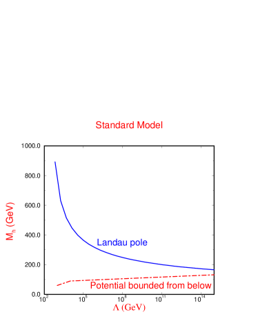
Figure 1: Theoretically allowed mass region for the Higgs boson as a function of the scale of new physics, $\Lambda$. The region above the solid line is forbidden because the quartic coupling, $\lambda(\Lambda)$, has a Landau pole. The region below the dot-dashed line is forbidden because the scalar potential is unbounded from below, $\lambda(\Lambda)<0$.

The alternate limit for the quartic coupling also gives an interesting limit on the Higgs boson mass. For small $\lambda$, the evolution with energy is

$$Q{d\lambda\over dQ}\sim{1\over 16\pi^{2}}\biggl{[}B-12g_{t}^{4}\biggr{]}\quad,$$ (8)

where

$$B = {3\over 4}\biggl{[}g^{4}+2g^{2}g^{\prime 2}+3g^{\prime 4}\biggr{]}$$

$$g_{t} = {m_{t}\over v}\quad.$$ (9)

($g$ and $g^{\prime}$ are the $SU(2)_{L}$ and $U(1)$ coupling constants, respectively, and $g_{t}$ is the top quark Yukawa coupling.) The large value of the top quark mass tends to drive the quartic coupling negative, thus destabilizing the potential. Eq. 8 can be easily solved for $\lambda(Q)$,

$$\lambda(Q)\sim\lambda(\Lambda)+{B-12g_{t}^{4}\over 16\pi^{2}}\log\biggl{(}{Q\over\Lambda}\biggl{)}\quad.$$ (10)

The requirement that the quartic coupling be always positive yields a lower bound on the Higgs boson mass,$\!{}^{{\bf?}}$

$$M_{h}^{2}>{v^{2}\over 8\pi^{2}}(12g_{t}^{4}-B)\log\biggl{(}{\Lambda\over M_{h}}\biggr{)}\quad.$$ (11)

This bound is the dot-dashed curve of Fig. 1. Including the $2$-loop evolution of all couplings and summing the large logarithms gives a lower bound on the Higgs mass slightly below that of Eq. 11. This bound is quite sensitive to the exact value of the top quark mass.$\!{}^{{\bf?}}$

The two bounds on the Higgs boson mass from the scale dependence of the potential are shown in Fig. 1 and we see that for any given scale $\Lambda$, the allowed region for the Higgs boson mass is quite restricted. For example, if there is no new physics beyond that of the Standard Model before the Planck scale, the allowed range is roughly,

$$130~{}GeV<M_{h}<170~{}GeV,$$ (12)

right in the intermediate mass Higgs boson range! The conclusion is clear: if the Standard Model describes physics below $10^{16}~{}-~{}10^{18}~{}GeV$, then the Higgs boson must be in the intermediate mass region.

A further indication of the importance of the intermediate mass Higgs boson is given by fits to electroweak data. Including data from LEP, SLD, CDF, and D0, the best fit for the Higgs boson mass is $\!{}^{{\bf?}}$

$$M_{h}=149^{+148}_{-82}~{}GeV\quad,$$ (13)

which gives a $95\%$ confidence level bound of

$$M_{h}<550~{}GeV\qquad.$$ (14)

Since the sensitivity of the electroweak data to the Higgs boson mass is only logarithmic, the bound is unfortunately extremely sensitive to which pieces of data are included in the fit. For example, removing the measurement of the hadronic width of the $Z$ boson increases the bound significantly.$\!{}^{{\bf?}}$ The results do seem to favor a Higgs boson in the intermediate range however. $\!{}^{{\bf?}}$

The above indications emphasize the crucial need to be able to experimentally probe the intermediate mass region. A detailed discussion of the experimental prospects for observing an intermediate mass Higgs boson in many different processes is given in Ref. $\!{}^{{\bf?},{\bf?}}$ and complements the discussion given here. In Section 2, we discuss the Higgs boson branching ratios, including as many radiative corrections as possible.$\!{}^{{\bf?}}$ We turn in Section 3 to a discussion of the production mechanisms at a hadron collider and survey the signatures at both the LHC and the Tevatron. More detailed discussions are contained in the chapters by S. Mrenna and J. Gunion. Section 4 has an overview of the properties of an intermediate mass Higgs boson at an $e^{+}e^{-}$ collider, while Sections 5 and 6 summarize the prospects for observing the intermediate mass Higgs boson at a $\mu^{+}\mu^{-}$ collider and in $\gamma\gamma$ collisions. Finally, Section 7 contains some conclusions.

2 Higgs Branching Ratios

2.1 Decays to Fermion Pairs

In the Higgs sector, the Standard Model is extremely predictive, with all couplings, decay widths, and production cross sections given in terms of the unknown Higgs boson mass. The Higgs couplings to fermions are proportional to fermion mass and the gauge invariant Yukawa couplings of the Higgs boson to fermions are,

$${\cal L}_{f}=-\lambda_{d}{\overline{Q}}_{L}\phi d_{R}-\lambda_{u}{\overline{Q}}_{L}\phi^{c}u_{R}+{\rm h.c.}$$ (15)

where $\phi^{c}=-i\tau_{2}\phi^{*}$ and ${\overline{Q}}_{L}=({\overline{u}}_{L},{\overline{d}}_{L})$. When the neutral Higgs boson obtains its vev, the Yukawa couplings are fixed in terms of the fermion masses, 

$$\lambda_{d} = {M_{d}\sqrt{2}\over v}$$

$$\lambda_{u} = {M_{u}\sqrt{2}\over v}\quad.$$ (16)

The measurements of the various Higgs decay channels will therefore serve to discriminate between the Standard Model and other models with more complicated Higgs sectors which may have different decay chains and Yukawa couplings. It is hence vital that we have reliable predictions for the branching ratios in order to verify the correctness of the Yukawa couplings of Eq.15.$\!{}^{{\bf?},{\bf?}}$

The dominant decays of the intermediate mass Higgs boson are into fermion- antifermion pairs. In the Born approximation, the width into charged lepton pairs is

$$\Gamma(h\rightarrow l^{+}l^{-})={G_{F}m_{l}^{2}\over 4\sqrt{2}\pi}M_{h}\beta_{l}^{3}\quad,$$ (17)

where $\beta_{l}\equiv\sqrt{1-4m_{l}^{2}/M_{h}^{2}}$ is the velocity of the final state leptons. The Higgs boson decay into quarks is enhanced by the color factor $N_{c}=3$ and also receives significant QCD corrections,

$$\Gamma(h\rightarrow q{\overline{q}})={3G_{F}m_{q}^{2}\over 4\sqrt{2}\pi}M_{h}\beta_{q}^{3}\biggl{(}1+{4\over 3}{\alpha_{s}\over\pi}\Delta_{h}^{QCD}\biggr{)}\quad,$$ (18)

where the QCD correction factor, $\Delta_{h}^{QCD}$, can be found in Ref. $\!{}^{{\bf?}}$.

For the intermediate mass Higgs boson, the ${\cal O}(\alpha_{s})$ corrections decrease the decay width for $h\rightarrow b{\overline{b}}$ by about a factor of $2$. A large portion of the corrections can be absorbed by expressing the decay width in terms of a running $b$-quark mass, $m_{b}(\mu)$, evaluated at the scale $\mu=M_{h}$. The decay width can then be written as,$\!{}^{{\bf?}}$

$$\Gamma(h\rightarrow q{\overline{q}})={3G_{F}\over 4\sqrt{2}\pi}m_{q}^{2}(M_{h}^{2})M_{h}\biggl{(}1+5.67{\alpha_{s}(M_{h}^{2})\over\pi}+\cdots\biggr{)},$$ (19)

where $\alpha_{s}(M_{h}^{2})$ is defined in the ${\overline{MS}}$ scheme with $5$ flavors and $\Lambda_{\overline{MS}}=150~{}GeV$. The ${\cal O}(\alpha_{s}^{2})$ corrections are also known in the limit $M_{h}>>m_{q}$.$\!{}^{{\bf?}}$

In leading log QCD, the running of the $b$ quark mass is,

$$m_{b}(\mu^{2})=M\biggl{[}{\alpha_{s}(M^{2})\over\alpha_{s}(\mu^{2})}\biggr{]}^{(-12/23)}\biggl{\{}1+{\cal O}(\alpha_{s}^{2})\biggr{\}},$$ (20)

where $m_{b}(M^{2})\equiv M$ implies that the running mass at the position of the propagator pole is equal to the location of the pole. For $m_{b}(m_{b}^{2})=4.2~{}GeV$, this yields an effective value $m_{b}((M_{h}=100~{}GeV)^{2})=3~{}GeV$. Inserting the QCD corrected mass into the expression for the width thus leads to a significantly smaller rate than that found using $m_{b}=4.2~{}GeV$.

The electroweak radiative corrections to $h\rightarrow q{\overline{q}}$ are not significant and amount to only a few percent correction.$\!{}^{{\bf?},{\bf?}}$ These can be neglected in comparison with the dominant QCD corrections.

The branching ratios for the dominant decays to fermion- antifermion pairs are shown in Fig. 2. The decrease in the $h\rightarrow f{\overline{f}}$ branching ratios at $M_{h}\sim 150~{}GeV$ is due to the turn-on of the $WW^{*}$ decay channel. For most of the region below the $W^{+}W^{-}$ threshold, the Higgs decays almost entirely to $b{\overline{b}}$ pairs, although it is possible that the decays to $\tau^{+}\tau^{-}$ will be useful.$\!{}^{{\bf?}}$ The other fermionic Higgs boson decay channels are almost certainly too small to be separated from the backgrounds. Even including the QCD corrections, the rates can be seen to roughly scale with the fermion masses and the color factor, $N_{c}$,

$${\Gamma(h\rightarrow b{\overline{b}})\over\Gamma(h\rightarrow\tau^{+}\tau^{-})}\sim{3m_{b}(M_{h}^{2})^{2}\over m_{\tau}^{2}},$$ (21)

and so a measurement of the branching ratios could serve to verify the correctness of the Standard Model couplings. The largest uncertainty is in the value of $\alpha_{s}$, which affects the running $b$ quark mass, as in Eq. 20 .

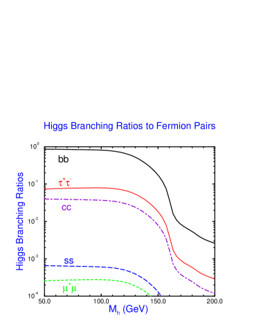
Figure 2: Branching ratios of the Standard Model Higgs boson to fermion-antifermion pairs, including QCD radiative corrections. We have taken $M_{t}=175~{}GeV$. The radiative corrections were computed using the program HDECAY.²²

2.2 Decays to Gauge Boson Pairs

The decay of the Higgs boson to gluons arises through fermion loops,$\!{}^{{\bf?}}$

$$\Gamma_{0}(h\rightarrow gg)={G_{F}\alpha_{s}^{2}M_{h}^{3}\over 64\sqrt{2}\pi^{3}}\mid\sum_{q}F_{1/2}(\tau_{q})\mid^{2}$$ (22)

where $\tau_{q}\equiv 4m_{q}^{2}/M_{h}^{2}$ and $F_{1/2}(\tau_{q})$ is defined,

$$F_{1/2}(\tau_{q})\equiv-2\tau_{q}\biggl{[}1+(1-\tau_{q})f(\tau_{q})\biggr{]}\quad.$$ (23)

The function $f(\tau_{q})$ is given by,

$$f(\tau_{q})=\left\{\begin{array}[]{ll}\biggl{[}\sin^{-1}\biggl{(}\sqrt{1/\tau_{q}}\biggr{)}\biggr{]}^{2},&\hbox{if~{}}\tau_{q}\geq 1\\ -{1\over 4}\biggl{[}\log\biggl{(}{x_{+}\over x_{-}}\biggr{)}-i\pi\biggr{]}^{2},&\hbox{ if~{}}\tau_{q}<1,\end{array}\right.$$ (24)

with

$$x_{\pm}=1\pm\sqrt{1-\tau_{q}}.$$ (25)

In the limit in which the quark mass is much less than the Higgs boson mass, (the relevant limit for the $b$ quark),

$$F_{1/2}\rightarrow{2m_{q}^{2}\over M_{h}^{2}}\log^{2}\biggl{(}{m_{q}\over M_{h}}\biggr{)}.$$ (26)

On the other hand, for a heavy quark, $\tau_{q}\rightarrow\infty$, and $F_{1/2}(\tau_{q})$ approaches a constant,

$$F_{1/2}\rightarrow-{4\over 3}.$$ (27)

It is clear that the dominant contribution to the gluonic decay of the Higgs boson is from the top quark loop and from possible new generations of heavy fermions. A measurement of this rate would serve to count the number of heavy fermions since the heavy fermions do not decouple from the theory.

The QCD radiative corrections from $h\rightarrow ggg$ and $h\rightarrow gq{\overline{q}}$ to the hadronic decay of the Higgs boson are large since they typically increase the width by more than $50\%$. The radiatively corrected width can be approximated by

$$\Gamma(h\rightarrow ggX)=\Gamma_{0}(h\rightarrow gg)\biggl{[}1+E{\alpha_{s}(\mu)\over\pi}\biggr{]}\quad,$$ (28)

where $E={215\over 12}-{23\over 6}\log(\mu^{2}/M_{h}^{2})$.$\!{}^{{\bf?},{\bf?}}$ The radiatively corrected branching ratio for $h\rightarrow ggX$ is the solid curve in Fig. 3.

The intermediate mass Higgs boson can also decay to vector boson pairs $VV^{*}$, ($V=W^{\pm},Z$), with one of the gauge bosons off-shell. The widths, summed over all available channels for $V^{*}\rightarrow f{\overline{f}}$ are:  $\!{}^{{\bf?}}$

$$\Gamma(h\rightarrow ZZ^{*}) = {g^{4}M_{h}\over 2048(1-x_{W})^{2}\pi^{3}}\biggl{(}7-{40\over 3}x_{W}+{160\over 9}x_{W}^{2}\biggr{)}F\biggl{(}{M_{Z}\over M_{h}}\biggr{)}$$

$$\Gamma(h\rightarrow WW^{*}) = {3g^{4}M_{h}\over 512\pi^{3}}F\biggl{(}{M_{W}\over M_{h}}\biggr{)}$$ (29)

where $x_{W}\equiv\sin^{2}\theta_{W}$ and

$$F(x) \equiv -\mid 1-x^{2}\mid\biggl{(}{47\over 2}x^{2}-{13\over 2}+{1\over x^{2}}\biggr{)}-3\biggl{(}1-6x^{2}+4x^{4}\biggr{)}\mid\ln(x)\mid$$ (30)

$$+3{1-8x^{2}+20x^{4}\over\sqrt{4x^{2}-1}}\cos^{-1}\biggl{(}{3x^{2}-1\over 2x^{3}}\biggr{)}\quad.$$

These widths can be significant when the Higgs boson mass approaches the real $W^{+}W^{-}$ and $ZZ$ thresholds, as can be seen in Fig. 3. The $WW^{*}$ and $ZZ^{*}$ branching ratios grow rapidly with increasing Higgs mass and above $2M_{W}$, the rate for $h\rightarrow W^{+}W^{-}$ is close to 1. The decay to $ZZ^{*}$ is roughly an order of magnitude smaller than the decay to $WW^{*}$ over much of the intermediate mass Higgs range due to the smallness of the neutral current couplings as compared to the charged current couplings.

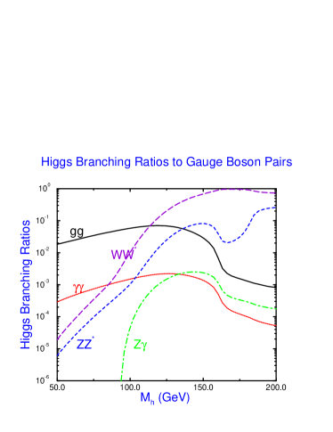
Figure 3: Branching ratios of the Standard Model Higgs boson to gauge boson pairs. The rates to $WW^{*}$ and $ZZ^{*}$ must be multiplied by the appropriate branching ratios for $W^{*}$ and $Z^{*}$ decays to $f{\overline{f}}$ pairs. We have taken $M_{t}=175~{}GeV$. The radiative corrections were computed using the program HDECAY.²²

The decay $h\rightarrow Z\gamma$ is not useful phenomenologically, so we will not discuss it here although the complete expression for the branching ratio can be found in Ref. $\!{}^{{\bf?}}$. On the other hand, the decay $h\rightarrow\gamma\gamma$ is an important mode for the Higgs search at the LHC. At lowest order, the branching ratio is, $\!{}^{{\bf?}}$

$$\Gamma(h\rightarrow\gamma\gamma)={\alpha^{2}G_{F}\over 128\sqrt{2}\pi^{3}}M_{h}^{3}\mid\sum_{i}N_{ci}Q_{i}^{2}F_{i}(\tau_{i})\mid^{2}$$ (31)

where the sum is over fermions and $W^{\pm}$ bosons with $F_{1/2}(\tau_{q})$ given in Eq. 23, and

$$F_{W}(\tau_{W})=2+3\tau_{W}[1+(2-\tau_{W})f(\tau_{W})]\quad.$$ (32)

$\tau_{W}=4M_{W}^{2}/M_{h}^{2}$, $N_{Ci}=3$ for quarks and $1$ otherwise, and $Q_{i}$ is the electric charge in units of $e$. The function $f(\tau_{q})$ is given in Eq. 24. The $h\rightarrow\gamma\gamma$ decay channel clearly probes the possible existence of heavy charged particles. (Charged scalars, such as those existing in SUSY models, would also contribute to the rate.)$\!{}^{{\bf?}}$

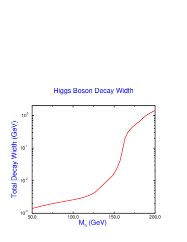
Figure 4: Total Higgs boson decay width in the Standard Model, including QCD radiative corrections. The turn-on of the $W^{+}W^{-}$ threshold at $M_{h}\sim 160~{}GeV$ is obvious. The top quark mass is fixed to $M_{t}=175~{}GeV$.

In the limit where the particle in the loop is much heavier than the Higgs boson, $\tau\rightarrow\infty$,

$$F_{1/2} \rightarrow -{4\over 3}$$

$$F_{W} \rightarrow ~{}7\quad.$$ (33)

The top quark contribution $(F_{1/2})$ is therefore much smaller than that of the $W$ loops $(F_{W})$ and so we expect the QCD corrections to be less important than is the case for the $h\rightarrow gg$ decay. In fact the QCD corrections to the total width for $h\rightarrow\gamma\gamma$ are quite small.$\!{}^{{\bf?}}$ The $h\rightarrow\gamma\gamma$ branching ratio is the dotted line in Fig. 3. For small Higgs masses it rises with increasing $M_{h}$ and peaks at around $2\times 10^{-3}$ for $M_{h}\sim 125~{}GeV$. Above this mass, the $WW^{*}$ and $ZZ^{*}$ decay modes are increasing rapidly with increasing Higgs mass and the $\gamma\gamma$ mode becomes tiny.

The total width for the intermediate mass Higgs boson is shown in Fig. 4. Below around $M_{h}\sim 150~{}GeV$, the Higgs boson is quite narrow with $\Gamma_{h}<10~{}MeV$. As the $WW^{*}$ and $ZZ^{*}$ channels become accessible, the width increases rapidly with $\Gamma_{h}\sim 1~{}GeV$ at $M_{h}\sim 200~{}GeV$. In the intermediate mass region, the Higgs boson width is too narrow to be resolved experimentally. The total width for the lightest neutral Higgs boson in the minimal SUSY model is typically much smaller than the Standard Model width for the same Higgs boson mass and so a measurement of the total width could serve to discriminate between the two models. The individual decay channels are also quite different in the Standard Model and in a SUSY model, as is discussed in the chapter by H. Haber.

We turn now to the production of the intermediate mass Higgs boson in hadronic interactions.

3 Higgs Production in Hadronic Interactions

3.1 Gluon Fusion

Lowest Order

An important production mechanism for the Higgs boson at hadron colliders is gluon fusion which proceeds through a quark triangle. This is the dominant contribution to Higgs boson production at the LHC for all $M_{h}<1~{}TeV$. The lowest order cross section for $gg\rightarrow h$ is,$\!{}^{{\bf?}}$

$${\hat{\sigma}}(gg\rightarrow h) = {\alpha_{s}^{2}\over 1024\pi v^{2}}\mid\sum_{q}F_{1/2}(\tau_{q})\mid^{2}\delta\biggl{(}1-{{\hat{s}}\over M_{h}^{2}}\biggr{)}$$ (34)

$$\equiv {\hat{\sigma}}_{0}(gg\rightarrow h)\delta\biggl{(}1-{{\hat{s}}\over M_{h}^{2}}\biggr{)}\quad,$$

where ${\hat{s}}$ is the gluon-gluon center of mass energy, $v=246~{}GeV$ and $F_{1/2}(\tau_{q})$ is defined in Eq. 23. In the heavy quark limit, $(M_{t}/M_{h})\rightarrow\infty$, the cross section becomes,

$${\hat{\sigma}}_{0}(gg\rightarrow h)\sim{\alpha_{s}^{2}\over 576\pi v^{2}}\quad.$$ (35)

This rate counts the number of heavy quarks and so could be a window into a possible fourth generation of quarks.

The Higgs boson production cross section at a hadron collider can be found by integrating the parton cross section with the gluon structure functions, $g(x)$,

$$\sigma_{0}(pp\rightarrow h)={\hat{\sigma}_{0}}\tau\int_{\tau}^{1}{dx\over x}g(x)g\biggl{(}{\tau\over x}\biggr{)},$$ (36)

where $\sigma_{0}$ is given in Eq. 34, $\tau\equiv M_{h}^{2}/S$, and $S$ is the hadronic center of mass energy.

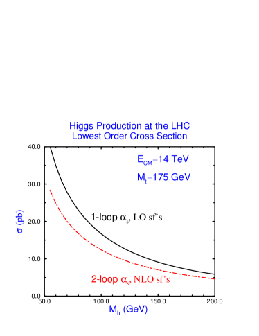
Figure 5: Cross section for gluon fusion, $gg\rightarrow h$, at the LHC using the lowest order parton cross section of Eq. 34. The solid (dot-dashed) line uses the one-loop (two-loop) expression for $\alpha_{s}(\mu)$, along with structure functions fitted to lowest order (next to lowest order) expressions for the data. The renormalization scale is $\mu=M_{h}$.

We show the rate obtained using the lowest order parton cross section of Eq. 34 in Fig. 5 for the LHC. When computing the lowest order result from Eq. 34, it is ambiguous whether to use the one- or two- loop equations for $\alpha_{s}(\mu)$ and which structure functions to use; a set fit to data using only the lowest order in $\alpha_{s}$ predictions or a set which includes some higher order effects. The difference between the equations for $\alpha_{s}$ and the different structure functions is ${\cal O}(\alpha_{s}^{2})$ and hence higher order in $\alpha_{s}$ when one is computing the “lowest order” result. In Fig. 5, we show two different definitions of the lowest order result and see that they differ significantly from each other. We will see in the next section that the result obtained using the $2$-loop $\alpha_{s}$ and NLO structure functions, but the lowest order parton cross section, is a poor approximation to the radiatively corrected rate. Fig. 5 takes the scale factor $\mu=M_{h}$ and the results are quite sensitive to this choice.

3.2 QCD Corrections to $gg\rightarrow h$

In order to obtain reliable predictions for the production rate, it is important to compute the $2-$loop QCD radiative corrections to $gg\rightarrow h$. The complete ${\cal O}(\alpha_{s}^{3})$ calculation is available in Refs. $\!{}^{{\bf?},{\bf?}}$. The analytic result is quite complicated, but the computer code including all QCD radiative corrections is readily available.$\!{}^{{\bf?}}$

For the intermediate mass Higgs boson, the result in the $M_{h}/M_{t}\rightarrow 0$ limit turns out to be an excellent approximation to the exact result and can be used in most cases. The heavy quark limit can be obtained from the gauge invariant effective Lagrangian,$\!{}^{{\bf?}}$

$${\cal L}=-{1\over 4}\biggl{[}1-{2\beta_{s}\over g_{s}(1+\delta)}{h\over v}\biggr{]}G_{\mu\nu}^{A}G^{A\mu\nu}-{M_{t}\over v}{\overline{t}}th\quad,$$ (37)

where $\delta=2\alpha_{s}/\pi$ is the anomalous mass dimension arising from the renormalization of the $t{\overline{t}}h$ Yukawa coupling constant, $g_{s}$ is the QCD coupling constant, and $G_{\mu\nu}^{A}$ is the color $SU(3)$ field. This Lagrangian can be derived using low energy theorems which are valid in the limit $M_{h}<<M_{t}$ and yields momentum dependent $ggh$, $gggh$, and $ggggh$ vertices which can be used to compute the rate for $gg\rightarrow h$ to ${\cal O}(\alpha_{s}^{3})$.

Since the $hgg$ coupling in the $M_{t}\rightarrow\infty$ limit results from heavy fermion loops, it is only the heavy fermions which contribute to $\beta_{s}$ in Eq. 37. To ${\cal O}(\alpha_{s}^{2})$, the heavy fermion contribution to the QCD $\beta$ function is,

$${\beta_{s}\over g_{s}}\mid{\rm heavy~{}fermions}=N_{H}{\alpha_{s}\over 6\pi}\biggl{[}1+{19\alpha_{s}\over 4}\biggr{]}\quad.$$ (38)

$N_{H}$ is the number of heavy fermions.

The parton level cross section for $gg\rightarrow h$ is found by computing the ${\cal O}(\alpha_{s}^{3})$ virtual graphs for $gg\rightarrow h$ and combining them with the bremsstrahlung process $gg\rightarrow gh$. The answer in the heavy top quark limit is,$\!{}^{{\bf?},{\bf?},{\bf?}}$

$${\hat{\sigma}}_{1}(gg\rightarrow hX)={\alpha_{s}^{2}(\mu)\over 576\pi v^{2}}\biggl{\{}\delta(1-z)+{\alpha_{s}(\mu)\over\pi}\biggl{[}h(z)+{\bar{h}}(z)\log\biggl{(}{M_{h}^{2}\over\mu^{2}}\biggr{)}\biggr{]}\biggr{\}}$$ (39)

where

$$h(z) = \delta(1-z)\biggl{(}\pi^{2}+{11\over 2}\biggr{)}-{11\over 2}(1-z)^{3}$$

$$+6\biggl{(}1+z^{4}+(1-z)^{4}\biggr{)}\biggl{(}{\log(1-z)\over 1-z}\biggr{)}_{+}-{\overline{h}}(z)\log(z)$$

$${\bar{h}}(z) = 6\biggl{(}{z^{2}\over(1-z)_{+}}+(1-z)+z^{2}(1-z)\biggr{)}$$ (40)

and $z\equiv M_{h}^{2}/{\hat{s}}$. The answer is written in terms of “+” distributions, which are defined by the integrals,

$$\int_{0}^{1}{f(x)\over(1-x)_{+}}\equiv\int^{1}_{0}{f(x)-f(1)\over 1-x}\quad.$$ (41)

The factor $\mu$ is an arbitrary renormalization point. To $\alpha_{s}^{3}$, the physical hadronic cross section is independent of $\mu$. There are also ${\cal O}(\alpha_{s}^{3})$ contributions from $q{\overline{q}}$, $qg$ and ${\overline{q}}g$ initial states, but these are numerically small.

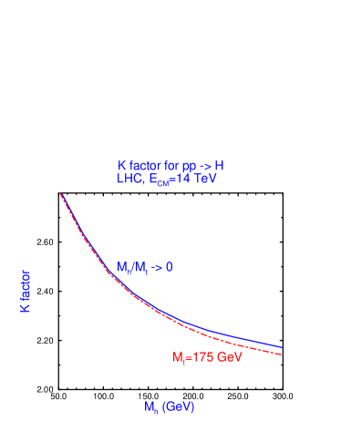
Figure 6: K factor as defined in Eq. 42. We have taken the renormalization scale $\mu=M_{h}$. The solid curve is the result obtained using the $M_{t}\rightarrow\infty$ limit, Eqs. 35 and 39, and the dot-dashed curve is the exact result from Ref. 17.

We can define a $K$ factor as

$$K\equiv{{\sigma}_{1}(pp\rightarrow hX)\over{\sigma}_{0}(pp\rightarrow h)}\quad,$$ (42)

where $\sigma_{1}(pp\rightarrow hX)$ is the ${\cal O}(\alpha_{s}^{3})$ radiatively corrected rate for Higgs production and $\sigma_{0}$ is the lowest order rate found from in Eq. 34. From Eq. 40, it is apparent that a significant portion of the corrections result from the rescaling of the lowest order result,

$$K\sim 1+{\alpha_{s}(\mu)\over\pi}\biggl{[}\pi^{2}+{11\over 2}+...\biggr{]}\quad.$$ (43)

Of course $K$ is not a constant, but depends on the renormalization scale $\mu$ as well as $M_{h}$. In Fig. 6, we show the $K$ factor obtained in the limit $M_{h}/M_{t}\rightarrow 0$, as well as the exact $K$ factor found in Ref. $\!{}^{{\bf?}}$. The radiatively corrected cross section ${\hat{\sigma}}_{1}$ should be convoluted with next-to-leading order structure functions, while it is ambiguous which structure functions and definition of $\alpha_{s}$ to use in defining the lowest order result, ${\hat{\sigma}}_{0}$, as discussed above. Fig. 6 uses the $2$-loop definition of $\alpha_{s}$ and NLO structure functions for both $\sigma_{0}$ and $\sigma_{1}$. A $K$ factor computed using lowest order structure functions and the one-loop definition of $\alpha_{s}$ for $\sigma_{0}$ would be smaller than that shown in Fig. 6, (as is obvious from Fig. 5).

The $K$ factor varies between $2$ and $3$ for the intermediate mass Higgs boson and so the QCD corrections significantly increase the rate from the lowest order result. It is evident from Fig. 6 that for the intermediate mass Higgs boson, the heavy top quark limit is an excellent approximation to the $K$ factor. The easiest way to compute the radiatively corrected cross section is therefore to calculate the lowest order cross section including the complete mass dependence of Eq. 34 and then to multiply by the $K$ factor computed in the $M_{t}\rightarrow\infty$ limit. This result will be extremely accurate.

The other potentially important correction to the $hgg$ coupling is the two-loop electroweak contribution involving the top quark, which is of ${\cal O}(\alpha_{S}G_{F}M_{t}^{2})$. In the heavy quark limit, the function $F_{1/2}(\tau_{q})$ of Eq. 23 receives a contribution, $\!{}^{{\bf?},{\bf?}}$

$$F_{1/2}(\tau_{q})\rightarrow F_{1/2}(\tau_{q})\biggl{(}1+{G_{F}M_{t}^{2}\over 16\sqrt{2}\pi^{2}}\biggr{)}\quad.$$ (44)

When the total rate for Higgs production is computed, the ${\cal O}(\alpha_{s}G_{F}M_{t}^{2})$ contribution is $<.2\%$ and so can be neglected. The ${\cal O}(\alpha_{s}G_{F}M_{t}^{2})$ contributions therefore do not spoil the usefulness of the $gg\rightarrow h$ mechanism as a means of counting heavy quarks.

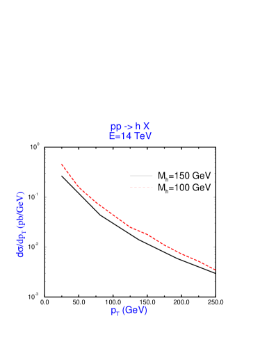
Figure 7: Higgs boson transverse momentum distribution from Eq. 45.

At lowest order the gluon fusion process yields a Higgs boson with no transverse momentum. At the next order in perturbation theory, gluon fusion produces a Higgs boson with finite $p_{T}$, primarily through the process $gg\rightarrow gh$. As $p_{t}\rightarrow 0$, the parton cross section diverges as $1/p_{T}^{2}$,$\!{}^{{\bf?}}$

$${d{\hat{\sigma}}\over d{\hat{t}}}(gg\rightarrow gh) = {\hat{\sigma}}_{0}{3\alpha_{s}\over 2\pi}\biggl{\{}{1\over p_{T}^{2}}\biggl{[}\biggl{(}1-{M_{h}^{2}\over{\hat{s}}}\biggr{)}^{4}+1+\biggl{(}{M_{h}^{2}\over{\hat{s}}}\biggr{)}^{4}\biggr{]}$$ (45)

$$-{4\over{\hat{s}}}\biggl{(}1-{M_{h}^{2}\over{\hat{s}}}\biggr{)}^{2}+{2p_{T}^{2}\over{\hat{s}}}\biggr{\}}\quad.$$

The hadronic cross section can be found by integrating Eq. 45 with the gluon structure functions. In Fig. 7, we show the $p_{T}$ spectrum of the Higgs boson at ${\cal O}(\alpha_{s}^{3})$. The event rate even at large $p_{T}$ is significant. This figure clearly demonstrates the singularity at $p_{T}=0$.

The terms which are singular as $p_{T}\rightarrow 0$ can be isolated and the integrals performed explicitly. For simplicity we consider only the $gg$ initial state.

$${d\sigma\over dp_{T}^{2}dy}(pp\rightarrow gh)\mid_{p_{T}^{2}\rightarrow 0}\sim{\hat{\sigma}}_{0}{3\alpha_{s}\over 2\pi}{1\over p_{T}^{2}}\biggl{[}6\log\biggl{(}{M_{h}^{2}\over p_{T}^{2}}\biggr{)}-2\beta_{0}\biggr{]}g(\tau e^{y})g(\tau e^{-y})+...$$ (46)

where $\tau=M_{h}^{2}/S$, $\beta_{0}=(33-2N_{L})/6$, and $N_{L}=5$ is the number of light flavors. Clearly when $p_{T}<<M_{h}$, the terms containing the large logarithms resulting from the multiple gluon emission must be summed. A consistent procedure for resumming the logarithms to next to leading order has been found by Collins, Soper, and Sterman. $\!{}^{{\bf?}}$ At an intermediate value of $p_{T}$, one must then switch from the resummed result to the perturbative result which is valid at high $p_{T}$. This results in a flattening of the $d\sigma/dp_{T}$ curve of Fig. 7 at low $p_{t}$.$\!{}^{{\bf?},{\bf?}}$

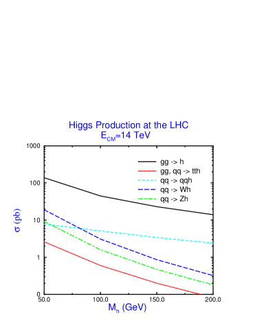
Figure 8: Contributions to $pp\rightarrow hX$ at the LHC, $E_{CM}=14~{}TeV$, including QCD radiative corrections for all processes except $t{\overline{t}}h$ production.

Fig. 8 shows the various contributions to Higgs boson production in the intermediate mass region at the LHC, including QCD corrections for all processes except $t{\overline{t}}h$ production. Gluon fusion (the solid curve) is obviously the dominant mechanism with a cross section between $10$ and $100~{}pb$ over the entire intermediate mass region. Vector boson fusion, $qq\rightarrow qqh$, (the short-dashed line) is an order of magnitude smaller than gluon fusion for the intermediate mass Higgs boson. Since it is not useful for Higgs searches in this region, we will not discuss it.

There are two particularly important decay modes for the experimental searches in the intermediate mass region at the LHC. For $M_{h}<125~{}GeV$, the best signal is from $h\rightarrow\gamma\gamma$. The branching ratio is larger than $10^{-3}$ for $80~{}GeV<M_{h}<120~{}GeV$ and so $100~{}fb^{-1}$ will produce $1000$’s of $h\rightarrow\gamma\gamma$ events. The Higgs signal is then a narrow bump in the $\gamma\gamma$ invariant mass spectrum. There is a very large irreducible background from two photon events, as well as a significant background from jets which are misidentified as photons. With $100~{}fb^{-1}$, ATLAS expects to probe $110~{}GeV<M_{h}<140~{}GeV$, while CMS estimates that it will be sensitive to $85~{}GeV<M_{h}<150~{}GeV$.$\!{}^{{\bf?}}$ The CMS detector will cover a larger range in Higgs mass, due to the expected excellence of its electromagnetic calorimeter. For the lower Higgs boson masses, the rate to $\gamma\gamma$ becomes extremely small (see Fig. 3) and the backgrounds become very large. One must hope that the unexplored region below $85~{}GeV$ will be probed at LEPII.

The $\gamma\gamma$ mode will also allow a precise measurement of the Higgs mass. For $M_{h}\sim 100~{}GeV$, ATLAS expects to measure $\Delta M_{h}\sim 1.4~{}GeV$, while CMS claims a slightly better precision. $\!{}^{{\bf?}}$ A more complete discussion of the physics capabilities of ATLAS and CMS to detect the Higgs boson in the $\gamma\gamma$ decay mode can be found in the chapter by J.  Gunion.

Above $M_{h}\sim 125~{}GeV$, the branching ratio to $h\rightarrow\gamma\gamma$ becomes too small to be useful and the best signal is from $h\rightarrow ZZ^{*}\rightarrow l^{+}l^{-}l^{\prime+}l^{\prime-}$. Above the $ZZ$ threshold, this is termed the “gold-plated” mode because it is so easy to observe. $\!{}^{{\bf?}}$ Below the $ZZ$ threshold, the irreducible backgrounds from $ZZ^{*}$ and $Z\gamma^{*}$ production are small and the dominant reducible backgrounds are from $t{\overline{t}}$ and $Zb{\overline{b}}$ production which can be efficiently eliminated with lepton isolation cuts. With $100~{}fb^{-1}$, both detectors expect that the smallest Higgs mass which they will be sensitive to in the $ZZ^{*}$ channel will be $M_{h}\sim 130~{}GeV$, while they will probe masses up to $M_{h}\sim 400-500~{}GeV$ in the $4$ charged lepton channel.$\!{}^{{\bf?}}$ To probe down to $M_{h}\sim 120~{}GeV$ in this mode will require several years of running at high luminosity. The ATLAS and CMS technical proposals contain numerous details.$\!{}^{{\bf?}}$

A measurement of both the $h\rightarrow\gamma\gamma$ and $h\rightarrow ZZ^{*}$ decay modes would be an important test of the $SU(2)$ symmetry of the Standard Model. The $h\rightarrow\gamma\gamma$ mode is dominated by the $W$ boson loop (see Eq. 33) and so is sensitive to the $hW^{+}W^{-}$ coupling, while the $h\rightarrow ZZ^{*}$ mode probes the $hZZ$ coupling. In the Standard Model, these couplings are related by,

$${g_{hWW}\over g_{hZZZ}}=\cos^{2}\theta_{W}\quad,$$ (47)

while the ratio of couplings is quite different in a supersymmetric model.

3.3 Associated Production, $pp(p{\overline{p}})\rightarrow Vh$.

The process $q{\overline{q}}\rightarrow Wh$ offers the hope of being able to tag the Higgs boson by the $W$ boson decay products.$\!{}^{{\bf?}}$ This process has the rate:

$${\hat{\sigma}}(q_{i}{\overline{q}}_{j}\rightarrow W^{\pm}h)={G_{F}^{2}M_{W}^{6}\mid V_{ij}\mid^{2}\over 6{\hat{s}}^{2}(1-M_{W}^{2}/{\hat{s}})^{2}}\lambda_{Wh}^{1/2}\biggl{[}1+{{\hat{s}}\lambda_{Wh}\over 12M_{W}^{2}}\biggr{]}$$ (48)

where $\lambda_{Wh}=1-2(M_{W}^{2}+M_{h}^{2})/{\hat{s}}+(M_{W}^{2}-M_{h}^{2})^{2}/{\hat{s}}^{2}$ and $V_{ij}$ is the Kobayashi-Maskawa angle associated with the $q_{i}{\overline{q}}_{j}W$ vertex. This process is sensitive to the $W^{+}W^{-}h$ coupling and so will be different in extensions of the Standard Model.

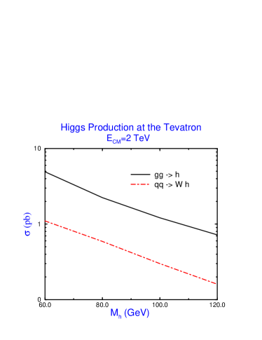
Figure 9: Next to leading order QCD predictions for Higgs boson production at the Tevatron. The dot-dashed line is the $W^{\pm}h$ production rate (summed over $W^{\pm}$ charges), while the solid line is the rate for Higgs production from gluon fusion.

Since this mechanism produces a relatively small number of signal events, (as can be seen clearly in Figs. 8 and 9), it is important to compute the rate as accurately as possible by including the QCD radiative corrections. This has been done in Ref. $\!{}^{{\bf?}}$, where it is shown that the cross section can be written as

$${d\sigma\over dq^{2}}(pp\rightarrow W^{\pm}h)=\sigma(pp\rightarrow W^{\pm*}){G_{F}M_{W}^{4}\over\sqrt{2}\pi^{2}(q^{2}-M_{W}^{2})^{2}}{\mid{\vec{p}}\mid\over\sqrt{q^{2}}}\biggl{(}1+{\mid{\vec{p}}\mid^{2}\over 3M_{W}^{2}}\biggr{)}$$ (49)

to all orders in $\alpha_{s}$. In Eq. 49, $W^{*}$ is a virtual $W$ with momentum $q$ and $\mid{\vec{p}}\mid=\sqrt{s}\lambda_{Wh}^{1/2}/2$ is the momentum of the outgoing $W^{\pm}$ and $h$. From Eq. 49, it is clear that the radiative corrections to $W^{\pm}h$ production are identical to those for the Drell-Yan process which have been known for some time.$\!{}^{{\bf?}}$ Using the DIS factorization scheme, the cross section at the LHC is increased by roughly $17\%$ over the lowest order rate. The QCD corrected cross section is relatively insensitive to the choice of renormalization and factorization scales. It is, however, quite sensitive to the choice of structure functions. The rate for $pp\rightarrow W^{\pm}h$ at the LHC is shown in Fig. 8 (the long-dashed curve) and is more than an order of magnitude smaller than the rate from gluon fusion. The rate for $pp\rightarrow Zh$ is smaller still.

The $Wh$ events can be tagged by identifying the charged lepton from the $W$ decay. Imposing isolation cuts on the lepton significantly reduces the background. At the LHC, there are sufficient events that the Higgs produced in association with a $W$ boson can be identified through the $\gamma\gamma$ decay mode.$\!{}^{{\bf?}}$ ATLAS claims a $4\sigma$ signal in this channel for $80~{}GeV<M_{h}<120~{}GeV$ with $100fb^{-1}$, (this corresponds to about $15$ signal events), while CMS hopes to find a $6-7\sigma$ effect in this channel. There are a large number of $Wh$ events with $W\rightarrow l\nu$ and $h\rightarrow b{\overline{b}}$, but unfortunately the backgrounds to this decay chain are difficult to reject and observation of this signal will probably require a high luminosity, $L=10^{33}/cm^{2}/sec$.$\!{}^{{\bf?}}$

Associated production of a Higgs boson with a $W^{\pm}$ boson can also potentially be observed at the Tevatron.$\!{}^{{\bf?}}$ For a $100~{}GeV$ Higgs boson, the lowest order cross section is $.2~{}pb$. Including the next-to-leading order corrections increases this to $.3~{}pb$, while summing over the soft gluon effects increases the NLO result by $2-3\%$. $\!{}^{{\bf?}}$ The next to leading order rate is shown in Fig. 9 and is much smaller that that from gluon fusion. At the Tevatron, the Higgs boson from $W^{\pm}h$ production must be searched for in the $b{\overline{b}}$ decay mode since the $\gamma\gamma$ decay mode produces too few events to be observable. The largest backgrounds are $Wb{\overline{b}}$ and $WZ$, along with top quark production. The background from top quark production is considerable smaller at the Tevatron than at the LHC, however. The Tevatron with $2-4~{}fb^{-1}$ will be sensitive to $M_{h}<M_{Z}$, a region which presumably will already be probed by LEPII. An upgraded Tevatron with higher luminosity (say $25~{}fb^{-1}$) may be able to probe a Higgs boson mass up to about $120~{}GeV$.$\!{}^{{\bf?},{\bf?}}$ This result depends critically on the $b$ tagging capabilities of the detectors, since it requires reconstructing the mass of both $b-$ jets.

3.4 Associated Production with Top, $pp(p{\overline{p}})\rightarrow t{\overline{t}}h$.

A potentially important mechanism for Higgs production at the LHC is the associated production with a $t{\overline{t}}$ pair. The $t{\overline{t}}h$ final state can result from either $q{\overline{q}}$ annihilation or from gluon-gluon scattering. From the dotted line in Fig. 8, we see that the rate is roughly $1~{}pb$ for $M_{h}\sim 100~{}GeV$. Although the rate is small, requiring an isolated charged lepton from the top decay significantly reduces the background and this decay may be useful. The $t{\overline{t}}h$ production mechanism is the only mode for which the QCD radiative corrections have not yet been calculated. A measurement of this channel will directly probe the $t{\overline{t}}h$ Yukawa coupling.

There are some interesting theoretical problems involved in calculating the rate for $t{\overline{t}}h$ production.$\!{}^{{\bf?}}$ The dominant contribution is from the gluon content of the proton. One can think about the $t{\overline{t}}$ quarks in the proton fusing to form a Higgs boson or about the full $gg\rightarrow t{\overline{t}}h$ process. Clearly, there is a potential for double counting if both the $t{\overline{t}}$ and $gg$ fusion production mechanisms are included. The prediction obtained using only the rate for $gg\rightarrow t{\overline{t}}h$ will be accurate everywhere except $M_{h}>>M_{t}$, where there will be large logarithms of the form $\log(M_{h}/M_{t})$. On the other hand, the fusion prediction, $t{\overline{t}}\rightarrow h$, will be accurate only if $M_{h}<M_{t}$. The resolution of the problem is to include the effects of gluon radiation in the leading logarithm approximation to all orders in $\alpha_{s}$ by using the heavy quark distribution functions, which include this radiation. However, to ${\cal O}(\alpha_{s})$ this logarithm already appears in the $gg\rightarrow t{\overline{t}}h$ process and hence must be subtracted from the heavy quark distribution functions. The answer obtained in this manner is consistent for all values of $M_{h}$ and $M_{t}$ and is shown in Fig. 8 for the LHC.

The best experimental limit on the Higgs boson mass at present comes from $Z$ decays at LEP and so we turn now to a discussion of producing the intermediate mass Higgs boson in $e^{+}e^{-}$ collisions.

4 Higgs Production in $e^{+}e^{-}$ Collisions

4.1 Higgs Production in $Z$ decays

Since the Higgs boson coupling to the electron is very small, $\sim m_{e}/v$, the $s-$channel production mechanism, $e^{+}e^{-}\rightarrow h$, is miniscule and the dominant production mechanism at LEP and LEPII for the intermediate mass Higgs boson is the associated production with a $Z$, $e^{+}e^{-}\rightarrow Z^{*}\rightarrow Zh$.

At the LEP collider with $\sqrt{s}\sim M_{Z}$, Higgs production could result from the on-shell decay $Z\rightarrow hf{\overline{f}}$. Neglecting fermion masses and the $Z$ boson width, the rate for Higgs production from $Z$ decay is given by,$\!{}^{{\bf?}}$

$${BR(Z\rightarrow hf{\overline{f}})\over BR(Z\rightarrow f{\overline{f}})} = {G_{F}M_{Z}^{2}\over 24\sqrt{2}\pi^{2}}\biggl{\{}{3y(y^{4}-8y^{2}+20)\over\sqrt{4-y^{2}}}\cos^{-1}\biggl{(}{y(3-y^{2})\over 2}\biggr{)}$$

$$-3(y^{4}-6y^{2}+4)\log y-{1\over 2}(1-y^{2})(2y^{4}-13y^{2}+47)\biggr{\}},$$

where $y\equiv M_{h}/M_{Z}$. The branching ratio for $Z\rightarrow hl^{+}l^{-}$ is shown in Fig. 10. It is clear that Higgs boson production in $Z$ decays can never be more than a $1\%$ effect on the total $Z$ width even for a very light Higgs boson.

The Higgs boson has been searched for in virtual $Z$ decays at the LEP collider. The primary decay mechanism used is $Z\rightarrow hl^{+}l^{-}$. The decay $Z\rightarrow h\nu{\overline{\nu}}$ is also useful since the branching ratio is six times larger than that of $Z\rightarrow hl^{+}l^{-}$. The strategy is to search through each range of Higgs boson masses separately by looking for the relevant Higgs decays. For example, a light Higgs boson, $M_{h}<2m_{e}$, necessarily decays to two photons. For $M_{h}\sim 1~{}MeV$, the Higgs lifetime is $c\tau\sim 10^{3}~{}cm$ and so the Higgs boson is long lived and escapes the detector without interacting. In this case a signal could be $e^{+}e^{-}\rightarrow Z\rightarrow l^{+}l^{-}h$ and the signal is $l^{+}l^{-}$ plus missing energy from the undetected Higgs boson. For each mass region, the appropriate Higgs decay channels are searched for. When the Higgs boson becomes heavier than twice the $b$ quark mass, it decays primarily to $b{\overline{b}}$ pairs and the signal resulting from leptonic $Z$ decays is then $e^{+}e^{-}\rightarrow Z\rightarrow l^{+}l^{-}h\rightarrow l^{+}l^{-}$ + jets. By a systematic study of Higgs boson masses and decay channels, the four LEP experiments have found the limit,$\!{}^{{\bf?}}$

$$M_{h}>65.2~{}GeV\quad.$$ (51)

Note that there is no region where light Higgs boson masses are allowed. The LEP limits thus obviate early studies of mechanisms such as $K\rightarrow\pi h$. The decay $Z\rightarrow h\gamma$, shown in Fig. 10, has too small a rate to be useful. A review of the LEP limits on the Standard Model Higgs boson is given in the chapter by Janot.

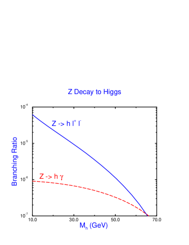
Figure 10: Branching ratio of the $Z$ boson to the Standard Model Higgs boson plus a charged lepton pair, $Z\rightarrow hl^{+}l^{-}$, or to $Z\rightarrow h\gamma$.

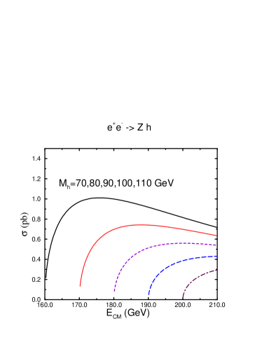
Figure 11: Born cross section for $e^{+}e^{-}\rightarrow Zh$ as a function of the center of mass energy, $E_{CM}$, and for various values of the Higgs boson mass.

4.2 Associated Production, $e^{+}e^{-}\rightarrow Zh$

At LEPII, the primary production mechanism for the Standard Model Higgs boson is $e^{+}e^{-}\rightarrow Zh$, in which a physical $Z$ boson is produced.$\!{}^{{\bf?}}$ The cross section is,

$${\hat{\sigma}}(e^{+}e^{-}\rightarrow hZ)={\pi\alpha^{2}\lambda_{Zh}^{1/2}[\lambda_{Zh}+12{M_{Z}^{2}\over s}](1+(1-4\sin^{2}\theta_{W})^{2}]\over 192s\sin^{4}\theta_{W}\cos^{4}\theta_{W}(1-M_{Z}^{2}/s)^{2}}$$ (52)

where

$$\lambda_{Zh}\equiv(1-{M_{h}^{2}+M_{Z}^{2}\over s})^{2}-{4M_{h}^{2}M_{Z}^{2}\over s}\quad.$$ (53)

The center of mass momentum of the produced $Z$ is $\lambda_{Zh}^{1/2}\sqrt{s}/2$ and the cross section is shown in Fig. 11 as a function of $\sqrt{s}$ for different values of the Higgs boson mass. The cross section peaks at $\sqrt{s}\sim M_{Z}+2M_{h}$.

The electroweak radiative corrections are quite small at LEPII energies.$\!{}^{{\bf?}}$ Photon bremsstrahlung can be important however since it is enhanced by a large logarithm, $\log(s/m_{e}^{2})$. The photon radiation can be accounted for by integrating the Born cross section of Eq. 52 with a radiator function $F$ which includes virtual and soft photon effects, along with hard photon radiation,$\!{}^{{\bf?}}$

$$\sigma={1\over s}\int ds^{\prime}F(x,s){\hat{\sigma}}(s^{\prime})$$ (54)

where $x=1-s^{\prime}/s$ and the radiator function $F(x,s)$ is known to ${\cal O}(\alpha^{2})$, along with the exponentiation of the infrared contribution,

$$F(x,s) = tx^{t-1}\biggl{\{}1+{3\over 4}t\biggr{\}}+\biggl{\{}{x\over 2}-1\biggr{\}}t+{\cal O}(t^{2})$$

$$t \equiv {2\alpha\over\pi}\biggl{[}\log\biggl{(}{s\over m_{e}^{2}}\biggr{)}-1\biggr{]}\quad.$$ (55)

Photon radiation significantly reduces the $Zh$ production rate from the Born cross section as shown in Fig. 12.

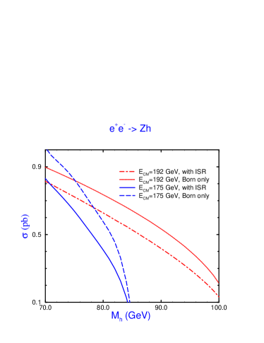
Figure 12: Effects of initial state radiation(ISR) on the process $e^{+}e^{-}\rightarrow Zh$. The curves labelled “Born only” are the results of Eq. 52, while those labelled “with ISR” include the photon radiation as in Eq. 54.

The intermediate mass Higgs boson will decay mostly to $b{\overline{b}}$ pairs, so the final state from $e^{+}e^{-}\rightarrow Zh$ will have four fermions. The dominant background is $Zb{\overline{b}}$ production, which can be efficiently eliminated by $b$-tagging almost up to the kinematic limit for producing the Higgs boson. LEPII studies estimate that with $\sqrt{s}=184~{}GeV$ and ${\cal L}=150pb^{-1}$, a Higgs boson mass of $87~{}GeV$ could be observed at the $5\sigma$ level.$\!{}^{{\bf?}}$ With higher energy, $\sqrt{s}=192~{}GeV$ and the same luminosity, masses up to $95~{}GeV$ could be reached. A higher energy $e^{+}e^{-}$ machine (such as an NLC with $\sqrt{s}\sim 500~{}GeV$) could push the Higgs mass limit to around $M_{h}\sim.7\sqrt{s}$.

Currently LEPII has data from both $\sqrt{s}=161~{}$ and $\sqrt{s}=172~{}GeV$. ALEPH has announced a preliminary limit on the Higgs boson mass of $\!{}^{{\bf?}}$

$$M_{h}>70.7~{}GeV\quad$$ (56)

from $10pb^{-1}$ of data. This analysis includes both hadronic and leptonic decay modes of the $Z$. Note how close this limit is to the kinematic boundary.

It is interesting to compare the upper bound on the Higgs mass from LEPII with the lowest mass reach of the $h\rightarrow\gamma\gamma$ process at the LHC. At LEPII, with $\sqrt{s}=192~{}GeV$, a mass of $M_{H}\sim 95~{}GeV$ will be probed, while the LHC will observe down to $M_{h}\sim 85~{}GeV$ in the $\gamma\gamma$ decay mode. We expect therefore that there will be no mass gap in the Higgs mass coverage, with the results from LEPII neatly meshing with those from the LHC. The higher energy at LEPII, $\sqrt{s}\sim 192~{}GeV$, is obviously necessary for this to be the case.

The cross section for $e^{+}e^{-}\rightarrow Zh$ is $s$-wave and so has a very steep dependence on energy and on the Higgs boson mass at threshold, as can be seen clearly in Fig. 11. This makes possible a precision measurement of the Higgs mass. Reconstructing the final state momenta at an NLC with $\sqrt{s}=500~{}GeV$ and assuming an SLD like detector could give a mass measurement with an accuracy of $\!{}^{{\bf?}}$

$$\Delta M_{h}\sim 180~{}MeV\sqrt{{50~{}fb^{-1}\over L}}\quad.$$ (57)

By measuring the cross section at threshold and normalizing to a second measurement above threshold in order to minimize systematic uncertainties, a $1\sigma$ measurement of the mass can be obtained $\!{}^{{\bf?}}$

$$\Delta M_{h}\sim 60\sqrt{{100fb^{-1}\over L}}\quad\quad{\rm for~{}~{}}M_{h}=100~{}GeV\quad,$$ (58)

where $L$ is the total integrated luminosity. The precision becomes worse for larger $M_{h}$ because of the decrease in the signal cross section. (Note that the luminosity at LEPII will not be high enough to perform this measurement.)

The angular distribution of the Higgs boson from the $e^{+}e^{-}\rightarrow Zh$ process is

$${1\over\sigma}{d\sigma\over d\cos\theta}\sim\lambda_{Zh}^{2}\sin^{2}\theta+{8M_{Z}^{2}\over s}$$ (59)

so that at high energy the distribution is that of a scalar particle,

$${1\over\sigma}{d\sigma\over d\cos\theta}\rightarrow{3\over 4}\sin^{2}\theta\quad.$$ (60)

If the Higgs boson were CP odd, on the other hand, the angular distribution would be $1+\cos^{2}\theta$. Hence the angular distribution is sensitive to the spin-parity assignments of the Higgs boson.

4.3 Higgs Production in Vector Boson Fusion, $VV\rightarrow h$

In $e^{+}e^{-}$ collisions the Higgs boson can also be produced by $W^{+}W^{-}$ fusion,$\!{}^{{\bf?},{\bf?}}$

$$e^{+}e^{-}\rightarrow W^{+}W^{-}\nu{\overline{\nu}}\rightarrow h\nu{\overline{\nu}},$$ (61)

and by $ZZ$ fusion,

$$e^{+}e^{-}\rightarrow ZZe^{+}e^{-}\rightarrow he^{+}e^{-}.$$ (62)

The fusion cross sections are easily found, $\!{}^{{\bf?}}$

$$\sigma_{VVh}={G_{F}^{3}M_{V}^{4}\over 64\sqrt{2}\pi^{3}}\int^{1}_{{M_{h}^{2}\over s}}dx\int^{1}_{x}{dy\over(1+s(y-x)/M_{V}^{2})^{2}}\biggl{(}(v^{2}+a^{2})^{2}f(x,y)+4v^{2}a^{2}g(x,y)\biggr{)}$$ (63)

where,

$$f(x,y) = \biggl{(}{2x\over y^{3}}-{1+2x\over y^{2}}+{2+x\over 2y}-{1\over 2}\biggr{)}\biggl{(}{w\over 1+w}-\log(1+w)\biggr{)}+{x\over y^{2}}{w^{2}(1-y)\over 1+w}$$

$$g(x,y) = \biggl{(}-{x\over y^{2}}+{2+x\over 2y}-{1\over 2}\biggr{)}\biggl{(}{w\over 1+w}-\log(1+w)\biggr{)}$$

$$w \equiv {y(sx-M_{h}^{2})\over M_{V}^{2}x}$$ (64)

and $v=a=\sqrt{2}$ for $e^{+}e^{-}\rightarrow W^{+}W^{-}\nu\overline{\nu}\rightarrow\nu{\overline{\nu}}h$ and $v=-1+4\sin^{2}\theta_{W},~{}a=-1$ for $e^{+}e^{-}\rightarrow ZZe^{+}e^{-}\rightarrow e^{+}e^{-}h$. The vector boson fusion cross sections are shown in Fig. 13 as a function of $\sqrt{s}$.

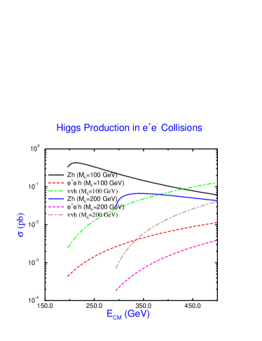
Figure 13: Higgs boson production in $e^{+}e^{-}$ collisions for $M_{h}=100$ and $200~{}GeV$.

The $ZZ$ fusion cross section is an order of magnitude smaller than the $W^{+}W^{-}$ fusion process due to the smaller neutral current couplings. This suppression is partially compensated for experimentally by the fact that the $e^{+}e^{-}h$ final state permits a missing mass analysis to determine the Higgs mass.

At an NLC, the cross section for vector boson fusion, $e^{+}e^{-}\rightarrow W^{+}W^{-}\nu{\overline{\nu}}\rightarrow h\nu{\overline{\nu}}$ and $e^{+}e^{-}\rightarrow Zh$ are of similar size for a $100~{}GeV$ Higgs boson. The fusion processes grow as $(1/M_{W}^{2})\log(s/M_{h}^{2})$, while the $s-$ channel process, $e^{+}e^{-}\rightarrow Zh$, falls as $1/s$ and so at high enough energy the fusion process will dominate, as can be seen in Fig. 13.

4.4 $e^{+}e^{-}\rightarrow t{\overline{t}}h$

Higgs production in association with a $t{\overline{t}}$ pair is small at an $e^{+}e^{-}$ collider. At $\sqrt{s}=500~{}GeV$, $20~{}fb^{-1}$ of luminosity would produce only $20$ events for $M_{h}=100~{}GeV$. The signature for this final state would be spectacular, however, since it would predominantly be $W^{+}W^{-}b{\overline{b}}b{\overline{b}}$, which would have a very small background. The $t{\overline{t}}h$ final state results almost completely from Higgs bremsstrahlung off the top quarks and could potentially yield a direct measurement of the $t{\overline{t}}h$ Yukawa coupling.$\!{}^{{\bf?}}$

5 Higgs Production in $\mu^{+}\mu-$ Collisions

An intermediate mass Higgs boson can also be probed via $\mu^{+}\mu^{-}\rightarrow Zh$ and the physics of this mechanism is almost identical to that of $e^{+}e^{-}\rightarrow Zh$. However, a $\mu^{+}\mu^{-}$ collider with high luminosity and narrow beam spread also offers the possibility of performing high precision measurements of the Higgs boson mass. Since the Higgs boson coupling is proportional to mass, the $s-$ channel process $\mu^{+}\mu^{-}\rightarrow h$ is considerably larger than the corresponding process in an $e^{+}e^{-}$ collider. The cross section for the resonant process $\mu^{+}\mu^{-}\rightarrow h\rightarrow X$ is,

$$\sigma_{h}(s)={4\pi\Gamma(h\rightarrow\mu^{+}\mu^{-})\Gamma(h\rightarrow X)\over(s-M_{h}^{2})^{2}+M_{h}^{2}\Gamma_{tot}^{2}}\quad,$$ (65)

where $\Gamma_{tot}$ is the total decay width of the Higgs boson. This process is obviously maximized when $\sqrt{s}\sim M_{h}$. One envisions discovering the Higgs boson via $e^{+}e^{-}\rightarrow Zh$ (or $\mu^{+}\mu^{-}\rightarrow Zh$) and then building a storage ring for a muon collider such that $\sqrt{s}\sim M_{h}$. At such a machine, precision studies of the Higgs mass and couplings could be performed. $\!{}^{{\bf?}}$

The crucial question is whether the energy spread of the beam is greater or smaller than the intrinsic width of the Higgs boson. Because the muon is so much heavier than the electron, there will be less initial state radiation and the beam energy resolution will typically be better in a muon collider than in an $e^{+}e^{-}$ collider. The beam energy resolution can be parameterized as a Gaussian with an rms deviation, $R$. This leads to an energy resolution, $\delta E$, of,

$$\delta E\sim 30~{}MeV\biggl{(}{R\over.05\%}\biggr{)}\biggl{(}{\sqrt{s}\over 100}\biggr{)}.$$ (66)

For a $\mu^{+}\mu^{-}$ collider, one expects values of $R\sim.1$ to $.01\%$, while for an $e^{+}e^{-}$ collider, $R\sim 1\%$. For $M_{h}<150~{}MeV$, the energy spread of the beam will be smaller than the Higgs width if $R<.05\%$, (See Fig. 4).

The physical cross section is then found by convoluting Eq. 65 with the energy resolution,

$$\sigma(s)=\int\sigma_{h}(s^{\prime})d\sqrt{s^{\prime}}exp^{-(\sqrt{s^{\prime}}-\sqrt{s})^{2}/(2\delta E)}{1\over\sqrt{2\pi}\delta E}\quad.$$ (67)

For $\delta E<<\Gamma_{tot}$, the cross section is

$$\sigma(s)\sim{\sqrt{2\pi}\pi\over M_{h}^{2}\delta E}\Gamma(h\rightarrow\mu^{+}\mu^{-}){\Gamma(h\rightarrow X)\over\Gamma_{tot}}\quad.$$ (68)

The $s$-channel Higgs cross section is shown in Fig. 14 for various values of $R$. The increase in the cross section with decreasing $R$ is clearly seen.

Detailed studies have estimated that with $R\sim.01\%$ and $7$ scan points centered around $\sqrt{s}\sim M_{h}$ (with a total luminosity of $3.5~{}fb^{-1}$) a measurement $\!{}^{{\bf?}}$

$$\Delta M_{h}\sim 4~{}MeV\quad$$ (69)

can be obtained. This is an order of magnitude smaller than that obtainable at an NLC (see Eq. 59). The height of the peak in Fig. 14 is a measure of $\Gamma_{tot}$ and the same $7$ scan points would yield a $10\%$ measurement of $\Gamma_{tot}$. A measuremtns of $\Gamma_{tot}$ is an important discriminator between the Standard Model Higgs boson and other non-Standard Model scalars.

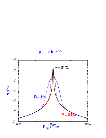
Figure 14: Cross section for resonant Higgs production in a $\mu^{+}\mu^{-}$ collider with $M_{h}=100~{}GeV$, for various values of the rms deviation in the energy spread, $R$.

6 Higgs Production in $\gamma\gamma$ Collisions

It is possible that an NLC with $\sqrt{s}\sim 500~{}GeV$ will be able to use back-scattered lasers to produce $\gamma\gamma$ or $e\gamma$ collisions with high energy and high luminosity. The $\gamma\gamma$ collisions may be useful for discovering the intermediate mass Higgs boson since the Higgs production rate is proportional to $\Gamma(h\rightarrow\gamma\gamma)$ and the full $\gamma\gamma$ center of mass energy goes into creating the Higgs boson.

The process we imagine observing is $\gamma\gamma\rightarrow h\rightarrow b{\overline{b}}$. The dominant background from $\gamma\gamma\rightarrow b{\overline{b}}$ is relatively easy to control. The signal is produced in a $J_{Z}=0$ state, while the background is mostly from $J_{Z}=2$. Therefore, polarizing the photons will efficiently discriminate against the background. There is also a significant background from “resolved photons”, where the effective process is $\gamma g$ or $gg\rightarrow b{\overline{b}}$. These resolved backgrounds are more severe for lower invariant masses and so we expect the lighter Higgs masses to be the hardest to see. Ref. $\!{}^{{\bf?}}$ estimates that $10fb^{-1}$ will allow a Higgs signal to be extracted in the range $110~{}GeV<M_{h}<140~{}GeV$ at a $500~{}GeV$ NLC.

A $\gamma\gamma$ collider will allow a direct measurement of the $h\gamma\gamma$ coupling, which is sensitive to all charged particles coupling to the Higgs boson. This coupling is also sensitive to the $W^{+}W^{-}\gamma$ and $W^{+}W^{-}h$ couplings and so provides a window to non-Standard Model gauge interactions.

An intermediate mass Higgs boson may also be probed in heavy ion collisions through the coherent $2$ photon production in the electromagnetic field of a nucleus with charge $Z$. Such interactions are enhanced by a factor of $Z^{4}$. Using calcium beams at the LHC, it may be possible to obtain a $3-4\sigma$ signal for a Higgs boson in the range $100<M_{h}<130~{}GeV$.$\!{}^{{\bf?}}$

7 Conclusion

The theoretical motivations for a Higgs boson in the intermediate mass region are extremely compelling, making it vital that this region be probed experimentally. If the Standard Model is the theory of electroweak interactions at energies all the way to the Planck scale, then the Higgs boson must exist in this region. Indirect electroweak measurements also support the validity of the intermediate mass hypothesis.

The combination of LEPII and the LHC should suffice to establish the existence of the Higgs boson if it is in the intermediate mass regime, although the region between $80$ and $90$ GeV is extremely challenging experimentally. The Higgs boson, once discovered, must also be measured in a variety of production channels and decay modes in order to confirm the Standard Model couplings.

References

References

- [1] J. Grivas,European Physical Society International Europhysics Conference on High Energy Physics, Brussels, Belgium, July 27 - August 2, 1995.
- [2] G. Cowen, CERN seminar, Feb. 25, 1997, http: //alephwww.cern.ch /ALPUB /seminar /Cowan-172-jam /cowan.html.
- [3] A. Hasenfratz, Quantum Fields on the Computer, (World Scientific, Singapore, 1992), ed. M. Creutz.
- [4] B.Lee, C. Quigg, and H. Thacker, Phys. Rev. D16 (1977) 1519; D. Dicus and V. Mathur, Phys. Rev. D7 (1973) 3111.
- [5] P. Chankowski, S. Pokorski, and J. Rosiek, Phys. Lett. B274 (1992) 191; J. Espinosa and M. Quiros, Phys. Lett. BB267 (1991) 27; H. Haber and R. Hempfling, Phys. Rev. D48 (1993) 4280; J. Ellis, G. Ridolfi, and F. Zwirner, Phys. Lett. B257 (1991) 83. See also the chapter by P. Chankowski and S. Pokorski, hep-ph/9702431.
- [6] C. Kolda, G. Kane, and J. Wells, Phys. Rev. Lett. 70 (1993) 2686.
- [7] N.Cabibbo, L. Maiani, G. Parisi, and R. Petronzio, Nucl. Phys. B158 (1979) 295; M. Sher, Phys. Rev. 179 (1989) 273; L. Maiani, G. Parisi, and R. Petronzio, Nucl. Phys. B136 (1978) 115; M.Lindner, Z. Phys. C31 (1986) 295; M. Lindner, M. Sher, and H. Zaglauer, Phys. Lett. 228 (1989) 139.
- [8] M. Sher, Phys. Lett. B317 (1993) 159; B331 (1994) 448; G. Altarelli and I. Isidori, Phys. Lett. B337 (1994) 141; J. Casa, J. Espinosa, and M. Quiros, Phys. Lett. B342 (1995) 171; C. Ford, D. Jones, P. Stephenson, and M. Einhorn, Nucl. Phys. B395 (1993) 17.
- [9] J. Espinosa and M. Quiros, Phys. Lett. 353B (1995) 257.
- [10] U. Baur, M. Demarteau et. al., Proceedings of the 1996 Snowmass Workshop, Snowmass, CO, June, 1996, hep-ph/9611334.
- [11] J. Rosner, Lectures given at The Cargese Summer Institute on Particle Physics, 1996, hep-ph/9610222.
- [12] J. Ellis, G. Fogli, and E. Lisi, Phys. Lett. B333 (1994) 118.
- [13] J. Gunion, A. Stange, and S. Willenbrock, to be published in Electroweak Symmetry Breaking and Beyond the Standard Model, (World Scientific, Singapore, 1997), ed. T. Barklow et. al., hep-ph/9602238.
- [14] J. Gunion et. al., Proceedings of the 1996 Snowmass Workshop, Snowmass, CO, June, 1996, hep-ph/9703330.
- [15] B. Kniehl, Phys. Rept. 240 (1994) 211.
- [16] A. Djouadi, Int. Journ. Mod. Phys. A10 (1995) 1, hep-ph/9406430.
- [17] M. Spira, A. Djouadi, D. Graudenz, and P. Zerwas, Nucl. Phys. B453 (1995) 17.
- [18] E. Braaten and J. Leveille, Phys. Rev. D22 (1980) 715; N. Sakai, Phys. Rev. D22 (1980) 2220; T. Inami and T. Kubota, Nucl. Phys. B179 (1981) 171; M. Drees and K.Hikasa, Phys. Lett. B240 (1990) 455; E. Gross, B. Kniehl and G. Wolf, Z. Phys. C63 (1994) 417; C66 (1995) 321 E.
- [19] A. Djouadi, M. Spira, and P. Zerwas, Z. Phys. C70 (1996) 427; Phys. Lett B264 (1991) 440.
- [20] S.Gorishny, A. Kataev, S. Larin, and L. Surguladze, Mod. Phys. Lett. A5 (1990) 2703.
- [21] J. Fleischer and F. Jegerlehner, Phys. Rev. D23 (1981) 2001; A. Dabelstein and W. Hollik, Nucl. Phys. C53 (1992) 507; B. Kniehl, Nucl. Phys. B376 (1992) 3.
- [22] M.Spira, Proceedings of AIHENP 96, Lausanne, Switzerland, Sept. 1996, CERN-TH-96-285, hep-ph/9610350.
- [23] R. Ellis et. al., Nucl. Phys. B297 (1988) 221.
- [24] J. Gunion et.al., The Higgs Hunter’s Guide (Addison Wesley, Menlo Park, 1990.)
- [25] T. Inami, T. Kubota, and Y. Okada, Z. Phys. C18 (1983) 69.
- [26] W.-Y. Keung and W. Marciano, Phys. Rev. D30 (1984) 248.
- [27] L. Bergstrom and G. Hulth, Nucl. Phys. B259 (1985) 137; R. Cahn, M. Chanowitz, and N. Fleishon, Phys. Rev. B82 (1979) 113.
- [28] A. Vainshtein, M. Voloshin, V. Zakharov, and M. Shifman, Sov. J. Nucl. Phys. 30 (1979) 711; M. Okun, Leptons and Quarks, (North-Holland, Amsterdam, 1982).
- [29] A. Djouadi, M. Spira, and P. Zerwas, Phys. Lett. B311 (1993) 255; S. Dawson and R. Kauffman, Phys. Rev. D47 (1993) 1264.
- [30] D. Graudenz, M. Spira and P. Zerwas, Phys. Rev. Lett.70 (1993) 1372.
- [31] S. Dawson, Nucl. Phys. B359 (1991) 283.
- [32] A. Djouadi and P. Gambino, Phys. Rev. Lett. 73 (1994) 2528
- [33] R . Kauffman, Phys. Rev. D44 (1991) 1415; I. Hinchliffe and S. Novaes, Phys. Rev. D38 (1988) 3475; C. Yuan, Phys. Lett. B283 (1992) 395.
- [34] J. Collins and D. Soper, Nucl. Phys. B193 (1981) 381; B213 (1983) 545 E; B197 (1982) 446; J. Collins, D. Soper, and G. Sterman, Nucl. Phys. B250 (1985) 199.
- [35] M. Kramer, E. Laenen, and M. Spira, CERN-TH-96-231, hep-ph/9611272.
- [36] Z. Kunszt, S. Moretti, and W. Stirling, DFTT-34/95, hep-ph/9611397.
- [37] ATLAS Technical Proposal, CERN/LHCC/94-43, LHCC/P2 (1994); CMS Technical Proposal, CERN/LHCC/94-38, LHCC/P1 (1994).
- [38] J. Gunion, G. Kane, and J. Wudka, Nucl. Phys. B299 (1988) 23.
- [39] T. Han and S. Willenbrock, Phys. Lett. B273 (1991) 167.
- [40] G. Altarelli, R. Ellis, and G. Martinelli, Nucl Phys. B157 (1979) 461; J. Kubar-Andre and F. Paige, Phys. Rev. D19 (1979) 221.
- [41] A. Stange, W. Marciano, and S. Willenbrock, Phys. Rev. D50 (1994) 4491; D49 (1994) 1354.
- [42] Report of the Tev2000 Study Group on Future Electroweak Physics at the Tevatron, eds. D. Amidei and R. Brock; FERMILAB-PUB-96-082, 1996.
- [43] S. Mrenna and C. Yuan, hep-ph/9703224.
- [44] D. Dicus and S. Willenbrock, Phys. Rev. D39 (1989)751; Z. Kunszt, Nucl. Phys. B247 (1984) 339.
- [45] D. Jones and S. Petcov, Phys. Lett. B84 (1979) 440.
- [46] F. Berends, physics at LEP1, CERN Yellow Report No 89-08, Geneva, 1989, Vol. 1, ed., G. Altarelli, R. Kleiss, and C. Verzegnassi; F. Berends, G. Burgess, and W. van Neervan, Nucl. Phys. B297 (1988) 429; B304 (1988) 921 E .
- [47] M. Carena, P. Zerwas, et. al., Higgs Physics, hep-ph/9602250.
- [48] V. Barger, M. Berger, J. Gunion, and T. Han, hep-ph/9612279; hep-ph/9602416; Phys. Rev. Lett. 75 (1995) 1462.
- [49] S. Dawson and J. Rosner, Phys. Lett. B148 (1984) 497.
- [50] A. Djouadi, J. Kalinowski and P. Zerwas, Z. Phys. C54 (1992) 255.
- [51] J. Gunion and H. Haber, Phy. Rev. D48 (1993) 5109; M. Baillargeon, G. Belanger, and F. Boudjema, Proceedings of Two Photon Physics from DANE to LEP200 and Beyond, Feb. 2-4, 1994, Paris, hep-ph/9405359.
- [52] E. Papageorgiu, Proceedings of 30th Rencontres do Moriond, Meribel les Allues, France, 1995, hep-ph/9507221.