Majorana Neutrinos and Gravitational Oscillation.

Abstract

We analyze the possibility of encountering resonant transitions of high energy Majorana neutrinos produced in Active Galactic Nuclei (AGN). We consider gravitational, electromagnetic and matter effects and show that the latter are ignorable. Resonant oscillations due to the gravitational interactions are shown to occur at energies in the PeV range for magnetic moments in the $10^{-17}\mu_{B}$ range. Coherent precession will dominate for larger magnetic moments. The alllowed regions for gravitational resonant transitions are obtained.

I Introduction

Majorana particles are natural representations of massive neutrinos since the most general mass term for a four component fermion field describes two Majorana particles with different masses. Majorana neutrinos also appear in many extensions of the minimal Standard Model; this is the case, for example, in SO(10) grand unified theories [1].

Neutrinos in general, and in particular Majorana neutrinos, can be used to probe the core of some of the most interesting cosmological objects. Due to their small cross sections these particles can stream out unaffected from even the most violent environments such as those present in Active Galactic Nuclei (AGN). The presence of several neutrino flavors and spin states modifies this picture: in their trek from their source to the detector the neutrinos can undergo flavor and/or spin transitions which can obscure some of the features of the source. Because of this, and due to the recent interest in neutrino astronomy (e.g. AMANDA, Nestor, Baikal, etc. [2]), it becomes important to understand the manner in which these flavor-spin transitions can occur, in the hope of disentangling these effects from the ones produced by the properties of the source. Without such an understanding it will be impossible to determine the properties of the AGN core using solely the neutrino flux received on Earth.

In a previous publication [3] we considered the effects of the AGN environment on the neutrino flux under the assumption that all neutrinos were of the Dirac type. In this complementary publication we will consider the case of Majorana neutrinos and provide a deeper phenomenological study of this system, concentrating on the dependence of the effects on the magnitude of the neutrino magnetic moment and on the energy dependence of the predicted neutrino fluxes.

The evolution of Majorana neutrinos in AGN is influenced both by its gravitational and electromagnetic interactions. The latter are due to the coupling with the magnetic field through a transition magnetic moment  . The combination of these effects leads to $\nu_{\mu}\rightarrow\bar{\nu_{e}}$ or $\bar{\nu_{\tau}}$ transitions. For simplicity we will deal with two neutrino species only, the extensions to three (or more) species is straightforward (though the analysis can become considerably more complicated [5]).

The paper is organized as follows. We start with a brief description of neutrino production and gravitational oscillation in AGN environment in section 2. This is followed by a calculation of transition and survival probabilities of oscillating neutrinos and the resulting flux modifications (sections 3 and 4). In section 5 we give our conclusions.

II Neutrino Oscillations in AGN

Active Galactic Nuclei (AGN) are the most luminous objects in the Universe, their luminosities ranging from $10^{42}$ to $10^{48}$ ergs$/$sec. They are believed to be powered by a central supermassive black hole whose masses are of the order of $10^{4}$ to $10^{10}M_{\odot}$.

High energy neutrino production in an AGN environment can be described using the so-called spherical accretion model [6] from which we can estimate the matter density and also the magnetic field (both of which are needed to study the evolution of the neutrino system). Neutrino production in this model occurs via the $\pi^{\pm}\rightarrow\mu^{\pm}\rightarrow e^{\pm}$ decay chain [6, 7] with the pions being produced through the collision of fast protons (accelerated through first-order diffusive Fermi mechanism at the shock [6]) and the photons of the dense ambient radiation field. These neutrinos are expected to dominate the neutrino sky at energies of 1 TeV and beyond [7].

Within this model the order of magnitude of the matter density $\rho$ for typical cases can be estimated at $10^{1}-10^{4}\;{\rm eV}^{4}$. The magnetic field, for reasonable parameters, is of the order of $10^{4}$ G  [3, 7, 8].

In order to determine the effective interactions of the Majorana neutrinos in an AGN environment we start, following [3], from the Dirac equation in curved space including their weak and electromagnetic interactions  

$$[ie^{\mu}_{a}\gamma^{a}(\partial_{\mu}+\omega_{\mu})-m+\not\!J\gamma_{5}+\mu\sigma^{ab}F_{ab}]\psi=0,$$ (1)

where $e^{\mu}_{a}$ are the tetrads, $\gamma^{a}$ the usual Gamma matrices, $m$ is the mass matrix, $\not\!J=J_{a}\gamma^{a}$ denotes the weak interaction current matrix, $\mu$ is the neutrino magnetic moment matrix, $F^{ab}$ the electromagnetic field tensor, $\sigma^{ab}={1\over 4}[\gamma_{a},\gamma_{b}]$; and the spin connection equals

$$\omega_{\mu}={1\over 8}[\gamma_{a},\gamma_{b}]e^{\nu a}e^{b}_{\nu;\mu}$$ (2)

where the semicolon denotes a covariant derivative. We used Greek indices ($\mu,\,\nu,\ldots$) to denote space-time directions, and Latin indices ($a,\,b,\ldots$) to denote directions in a local Lorentzian frame.

The method of extracting the effective neutrino Hamiltonian from (1) is studied in detail in [3]. We will therefore provide only a brief description of the procedure for completeness.

The first step of the semiclassical approximation is to consider a classical geodesic $\bar{x}^{\mu}(l)$ parameterized by an affine parameter $l$. Along this curve we construct three vector fields $\nu^{\mu}_{A}(l),\,A=1,2,3$ such that $\bar{x}+\nu_{A}\xi^{A}$ satisfies the geodesic differential equation to first order in the $\xi^{A}$. We then use $\{l,\xi^{A}\}$ as our coordinates (see, for example, [9]).

Next we consider the classical action as a function of the coordinates which satisfies the relation $p_{\mu}=\partial S/\partial x^{\mu}$ ($p$ is the classical momentum), and define a spinor $\chi$ via the usual semiclassical relation

$$\psi=e^{iS}\chi$$ (3)

In our calculations it proves convenient to define a time-like vector $\stackrel{{\scriptstyle\perp}}{{p}}$${}^{\;\mu}$ corresponding to the component of momentum $p$ orthogonal to the $\nu^{\mu}_{A}$

$${\mbox{\raisebox{-1.42271pt}{$\stackrel{{\scriptstyle\perp}}{{p}}$}}}{\mbox{\raisebox{0.28436pt}{${}^{\;\mu}$}}}=p^{\mu}-c_{A}(N^{-1})^{AB}\nu^{\mu}_{B};\qquad N_{AB}=\nu^{\mu}_{A}\nu^{\nu}_{B}g_{\mu\nu}$$ (4)

It can be shown that $c_{A}$ are constants [3]. We denote by $R$ the length-scale of the metric, so that, for example, $\omega_{\mu}\sim{1/R}$; and let $P$ be the order of magnitude of the momentum of the neutrinos. We then make a double expansion of $\chi$, first in powers of $\xi$ and then in powers of $1/pR$. We substitute these expressions into the Dirac equation and demand that each term vanish separately.

It is then possible to reduce the resulting equations to a Schrödinger-like equation involving only $\chi$ which reads

$$i\dot{\chi} = \tilde{H}_{\rm eff}\;\chi$$ (5)

$$\tilde{H}_{\rm eff} = -{1\over 2}(\not\!p+m)\left(i\gamma^{a}\bar{e}^{\mu}_{a}\bar{\omega}_{\mu}+\not\!\bar{J}\gamma_{5}\right)+{1\over 2}m^{2}-{i\over{2\not\!{\mbox{\raisebox{-1.42271pt}{$\stackrel{{\scriptstyle\perp}}{{p}}$}}}}}\dot{\not\!p}+{i\over 2}{\not\!\bar{\Upsilon}}^{A}{\not\!\bar{\lambda}}_{A}+\mu_{t}\sigma^{ab}F_{ab},$$ (6)

where,

$$\not\!\lambda_{A} = {1\over 2}\dot{N}_{AB}\not\!\Upsilon^{B}-\bar{e}^{\mu}_{a;\nu}p_{\mu}\nu^{\nu}_{A}\gamma^{a},$$ (8)

$$\not\!\Upsilon^{A} = (N^{-1})^{AB}\left(\nu_{\mu B}-{c_{B}{\mbox{\raisebox{-1.42271pt}{$\stackrel{{\scriptstyle\perp}}{{p}}$}}}_{\mu}\over{{\mbox{\raisebox{-1.42271pt}{$\stackrel{{\scriptstyle\perp}}{{p}}$}}}{\mbox{\raisebox{0.28436pt}{${}^{\;2}$}}}}}\right)\bar{e}^{\mu}_{a}\gamma^{a}.$$ (9)

(the over-bar indicates that the quantities are evaluated on the geodesic: $x=\bar{x}(l)$). Eqn. (LABEL:schr) determines the evolution of the 8-component (for two flavors) spinor $\chi$. We are interested, however only in the 4-components representing the spinors with positive momenta [3] (i.e. those directed from the source to the observer). Projecting $\tilde{H}_{\rm eff}$ into this 4-dimensional subspace yields the effective Hamiltonian $H_{\rm eff}$ for the states of interest

$$\ H_{\rm eff}=i\dot{\alpha}+{1\over 2}m^{2}+p\cdot J_{\rm eff}\,\left(\begin{array}[]{cc}1&0\\ 0&-1\end{array}\right)+\mu_{t}\sqrt{{\mbox{\raisebox{-1.42271pt}{$\stackrel{{\scriptstyle\perp}}{{p}}$}}}\cdot p}\,\left(\begin{array}[]{cc}0&B^{*}\\ B&0\end{array}\right)$$ (10)

where $B$ denotes the magnetic field and the effective current $J_{\rm eff}$ is defined by

$$J_{\rm eff}^{a}=J_{W}^{a}-J_{G}^{a}$$ (11)

in terms of the weak-interaction current $J_{W}^{a}$ and the “gravitational current”

$$J_{G}^{a}={1\over 4}\epsilon^{abcd}\bar{\lambda}_{fcd}\left(\eta^{f}_{b}+{2p^{f}{\mbox{\raisebox{-1.42271pt}{$\stackrel{{\scriptstyle\perp}}{{p}}$}}}_{b}\over{\mbox{\raisebox{-1.42271pt}{$\stackrel{{\scriptstyle\perp}}{{p}}$}}}{\mbox{\raisebox{0.28436pt}{${}^{\;2}$}}}}\right),$$ (12)

where

$$\lambda_{fcd}=(e_{f\mu,\nu}-e_{f\nu,\mu})e^{\mu}_{c}e^{\nu}_{d},\qquad\eta^{ab}=diag(1,-1,-1,-1).$$ (13)

The term $\dot{\alpha}$ in (10) is flavor and spin diagonal and can be eliminated by redefining the overall phase of $\chi$ with no observable consequences.

The evolution of Majorana neutrinos through matter in the presence of strong gravitational fields incorporating magnetic effects is thus,

$$i{d\over dl}\left(\begin{array}[]{c}\nu_{e}\\ \nu_{\mu}\\ {\bar{\nu}_{e}}\\ {\bar{\nu}_{\mu}}\end{array}\right)=H_{\rm eff}\left(\begin{array}[]{c}\nu_{e}\\ \nu_{\mu}\\ {\bar{\nu}_{e}}\\ {\bar{\nu}_{\mu}}\end{array}\right)$$ (14)

where $l$ is the affine parameter   and $H_{\rm eff}$ is the $4\times 4$ matrix containing the effects of the weak, electromagnetic and gravitational neutrino interactions, explicitly

$$H_{\rm eff}=\left(\begin{array}[]{cccc}\vspace{0.5cm}p\cdot J_{\rm eff}&{1\over 4}\Delta m^{2}\sin 2\vartheta&0&E\mu_{t}B^{\ast}\\ \vspace{0.5cm}{1\over 4}\Delta m^{2}\sin 2\vartheta&\qquad p\cdot J_{\rm eff}+{1\over 2}\Delta m^{2}\cos 2\vartheta&-E\mu_{t}B^{\ast}&0\\ \vspace{0.5cm}0&-E\mu_{t}B&-p\cdot J_{\rm eff}&{1\over 4}\Delta m^{2}\sin 2\vartheta\\ E\mu_{t}B&0&{1\over 4}\Delta m^{2}\sin 2\vartheta&\qquad-p\cdot J_{\rm eff}+{1\over 2}\Delta m^{2}\cos 2\vartheta\\ \end{array}\right)\vspace{0.5cm}$$ (15)

where $\vartheta$ is the neutrino mixing angle, $\Delta m^{2}=m^{2}_{1}-m^{2}_{2}$, $E$ the energy of the particle, $B=B_{1}+iB_{2}$ where $B_{1,2}$ are the AGN magnetic field components perpendicular to the direction of motion, and $\mu_{t}$ the transition magnetic moment. It is worth noting that, in contrast to the Dirac case, antineutrinos exhibit matter interactions. This Hamiltonian includes gravitational as well as electroweak effects; the latter have been studied previously (see, for example, [10]).

In our calculations we will use the Kerr metric to allow for the possibility of rotation of the central AGN black hole (we also have assumed that the accreting matter generates a small perturbation of the gravitational field). The metric for a Kerr black hole contains two parameters, $r_{g}$, the horizon radius and $a$ the total angular momentum of the black hole per unit mass. The geodesics in this gravitational field have three constants of the motion, commonly denoted by $E$, $L$ and $K$. The first corresponds to the energy, the second to the angular momentum along the black-hole rotation axis; the third constant $K$ has no direct interpretation, but is associated with the total angular momentum [11].

Using the AGN models mentioned above we can compare the weak interaction current $J_{W}$, to $J_{G}$, its gravitational counterpart. The orders of magnitude are,

$$J_{W}={G_{F}\;\rho\over m_{p}}\sim\left(10^{-33}\;\rho_{\rm eV}\right)\;\;{\rm eV}^{-1},\qquad J_{G}\sim R^{-1}$$ (16)

where $G_{F}$ is the Fermi coupling constant, $m_{p}$ the proton rest mass and $\rho_{\rm eV}$ is the density in ${\rm eV}^{4}$ units which for typical cases is $10^{1}-10^{4}\;$ [7]. Taking $R\sim r_{g}$, the gravitational current part is found to dominate the weak current part for all relevant values of $r_{g}\;(10^{14}\;{\rm to}\;10^{20}{\rm eV^{-1}})$. In the following we will drop $J_{W}$.

Setting $J_{W}=0$, $J_{\rm eff}$ can be written in terms of a dimensionless function $f$,

$$|p\cdot J_{\rm eff}|=Er_{g}^{-1}f(r/r_{g},\theta,j,k,a/r_{g}).$$ (17)

where we have chosen normalized parameters

$$j={L\over Er_{g}},\qquad k={K\over(Er_{g})^{2}}$$ (18)

We have plotted $|p\cdot J_{eff}|$ in figures 1 and 2 for some typical parameter values.

Using (15) we can determine the AGN regions where resonant transitions occur. These resonances are governed by the $2\times 2$ submatrices of (15) for each pair of states. The two possible resonances  are obtained by equating the diagonal terms for each submatrix and give rise to the following resonance conditions

$${1\over 4}\Delta m^{2}\cos 2\vartheta = p\cdot J_{G}\quad\qquad(\nu_{e}\;\rightarrow\;\bar{\nu}_{\mu})$$ (19)

$${1\over 4}\Delta m^{2}\cos 2\vartheta = -p\cdot J_{G}\quad\qquad(\nu_{\mu}\;\rightarrow\;\bar{\nu}_{e})$$ (20)

As can clearly be seen from the above two equations the resonant transitions do not occur simultaneously. We have considered electron and muon neutrinos, similar results hold for any other pair of flavors.

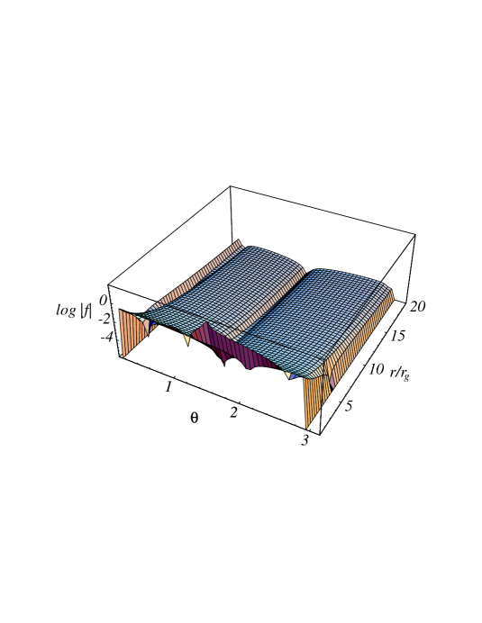
FIG. 1.: Plot of $\ln|f|$, see (17), for $j=0.15,\;k=0.4$, $a/r_{g}=0.4$ and $M=10^{8}M_{\odot}$.

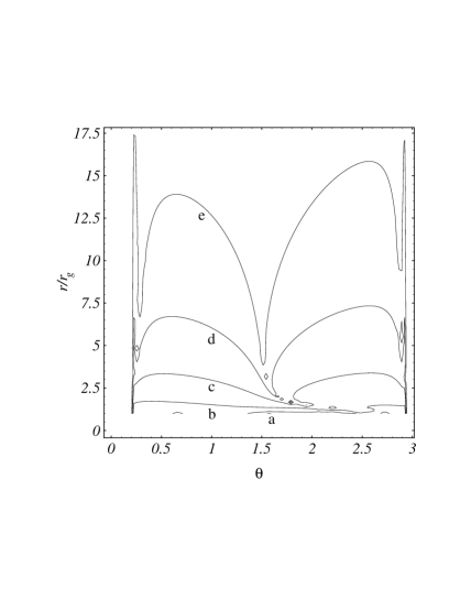
FIG. 2.: Contour-plot of $f$, see (17), for$j=0.15,\;k=0.4$, $a/r_{g}=0.4$ for the case $M=10^{8}M_{\odot}$. The contours a,b,c,d,e correspond respectively to $f=\pm 1,\,\pm 10^{-1},\,\pm 10^{-2},\,\pm 10^{-3},\,\pm 10^{-4}$, (positive values for $0\leq\theta\leq\pi/2$, negative values for $\pi/2\leq\theta\leq\pi$).

Resonances occur provided $f$ is comparable to $\pm\Delta m^{2}\cos 2\vartheta r_{g}/E$ as can be seen from (19) and (20). As suggested by figures 1 and 2, we have verified that, just as in the Dirac case [3], for almost all values of $j$, $k$ and $a$ the neutrinos will undergo resonances at a radius $r$ (the precise value of which changes with $\theta$) for all relevant values of $\Delta m^{2}$ (in the range $10^{-2}$ to $10^{-10}{\rm eV^{2}}$) provided $E$ is large enough ($>10^{8}{\rm eV}$ in this case) . This implies that practically all Majorana neutrinos will experience resonances provided their energy is large enough. As an example for $E\sim 1$ PeV and $\Delta m^{2}_{12}\sim 10^{-6}$eV² (Solar large angle solution), the resonance contour corresponds to (d) in Fig. 2.

III Probabilities for Allowed Transitions

In this section we evaluate the survival and transition probabilities of neutrino transitions and look into the region in parameter space where resonant neutrino transitions occur. The average probabilities for oscillating neutrinos (including non-adiabatic effects) produced in a region with mixing angle $\vartheta_{G}$, and detected in vacuum where the mixing angle is $\vartheta$, are given in general by [12, 13]

$$P(\nu_{\mu}\rightarrow\nu_{\mu})={1\over 2}+\left({1\over 2}-P_{LZ}\right)\cos 2\vartheta_{G}\cos 2\vartheta$$ (21)

and

$$P(\nu_{\mu}\rightarrow\bar{\nu}_{e})={1\over 2}-\left({1\over 2}-P_{LZ}\right)\cos 2\vartheta_{G}\cos 2\vartheta$$ (22)

where $\vartheta_{G}$ is the gravitational mixing angle,

$$\tan 2\vartheta_{G}=\left.{4E\,\mu_{t}B\over\Delta m^{2}\cos 2\vartheta+4p\cdot J_{G}}\right|_{\rm prod.}$$ (23)

(evaluated at the production point) and $\mu_{t}$ is the transition magnetic moment, $B$ the magnetic field, $\Delta m^{2}$ the usual mass difference parameter and $J_{G}$ given in eqn.(17). $P_{LZ}$ is the Landau Zener probability

$$P_{LZ}=\exp\left\{-2\pi^{2}\,{\beta^{2}\over\alpha}\right\}$$ (24)

where

$$\beta=E\mu_{t}B|_{\rm res}\qquad\alpha={d\over dl}\left[-p\cdot J_{\rm eff}\right]_{\rm res}$$ (25)

The condition for adiabatic resonances to induce an appreciable transition probability is $2\pi^{2}\beta^{2}\geq\alpha$ which in terms of the magnetic moment implies

$$\mu_{t}\geq{1\over EB}\left|{\Delta m^{2}\over 2\pi^{2}\Lambda}\right|^{1/2}=\mu^{\rm res}_{\rm min}$$ (26)

where $\Lambda=\left|dl/d\ln\left(p\cdot J_{\rm eff}\right)\right|$ is a measure of the scale of the gravitational field (divided by $E$), and we have assumed that the magnetic field remains constant over an interval of magnitude $\sim\Lambda$. In order to exhibit the energy dependence of $\mu^{\rm res}_{\rm min}$ we estimate $\Lambda\sim r_{g}\,/E$ whence

$$\mu^{\rm res}_{\rm min}\sim{1\over B}\left|{\Delta m^{2}\over 2\pi^{2}r_{g}E}\right|^{1/2}$$ (27)

Using equations (21) and (22) we can then calculate the survival and transition probabilities for the neutrinos. The results depend on the particular geodesic followed by the neutrinos, that is, it depends on the parameters $E$ as well as $j$ and $k$ defined in (18). The results are also dependent on the characteristics of the gravitational field and its environment through the magnetic field, the horizon radius $r_{g}$ and the angular momentum parameter $a$. Finally there is also an important dependence on the neutrino parameters $\Delta m^{2}$ and $\mu_{t}$.

For the study of the probabilities there are two regions of interest (assuming (26) is satisfied). If $p\cdot J_{G}>(E\>\mu_{t}B)$ the system experiences adiabatic resonances whenever the energy is such that $\vartheta_{G}\sim\pi/2$. If $p\cdot J_{G}<(E\>\mu_{t}B)$ the system will exhibit coherent precession  [14] if $E\>\mu_{t}B>\Delta m^{2}$ or no appreciable transitions if $E\>\mu_{t}B<\Delta m^{2}$.

For a study of the resonance scenario we will choose $\mu_{t}=10^{-17}\mu_{B}$ which is amply allowed by the current experimental and astrophysical constraints and still ensures neutrino adiabatic resonant transitions for all $\Delta m^{2}$ values considered provided $E$ is sufficiently large . This value is smaller than the one usually considered in the literature due to our being concerned with energies in the PeV range and the fact that $\mu^{\rm res}_{\rm min}$ decreases as $1/\sqrt{E}$. For larger values of $\mu_{t}$ transitions are dominated by coherent precession (provided $E\mu_{t}B>\Delta m^{2}$).

Using expressions (21) and (22) we obtained the probabilities of gravitationally induced adiabatic transitions, the results are presented in Fig. 3. If $E=E_{R}$ is the resonant energy (for a particular choice of parameters) then at that energy $\cos 2\vartheta_{G}\sim 0$. If $E<E_{R}$ the transition probability approaches the vacuum value $P(\nu_{\mu}\rightarrow\bar{\nu}_{e})=\sin^{2}2\vartheta$. For $E>E_{R}$, and for the value of $\mu_{t}$ chosen, $\vartheta_{G}\rightarrow\pi/2$ and the transition probability approaches $P(\nu_{\mu}\rightarrow\bar{\nu}_{e})=\cos^{2}\vartheta$, which is $\sim 1$; this is our region of interest. Equation (26) is satisfied in Fig. 3 when $P(\nu_{\mu}\rightarrow\bar{\nu}_{e})$ approaches 1 and $P(\nu_{\mu}\rightarrow\bar{\nu}_{\mu})$ approaches zero which corresponds to conditions for adiabatic resonant transitions. The energy $E_{R}$ denotes the adiabatic threshold energy between no gravitational effects and adiabatic resonant conversion. This behavior is illustrated in Fig. 3. Fig. 4 shows the dependence of the probabilities on $r$ and $\theta$.

FIG. 3.: Plot of the persistence (left) and transition (right) probabilities as functions of $E(\rm eV)$ for $\mu_{t}=10^{-17}\mu_{B}$, $r/r_{g}=6$, $\theta=\pi/2$, $j=0.15$, $k=0.4$, $a/r_{g}=0.4$ and $M=10^{8}M_{\odot}$. The curves a,b,c,d,e correspond to $\Delta m^{2}=10^{-10},10^{-8},10^{-6},10^{-4},10^{-2}{\rm eV}^{2}$ respectively.

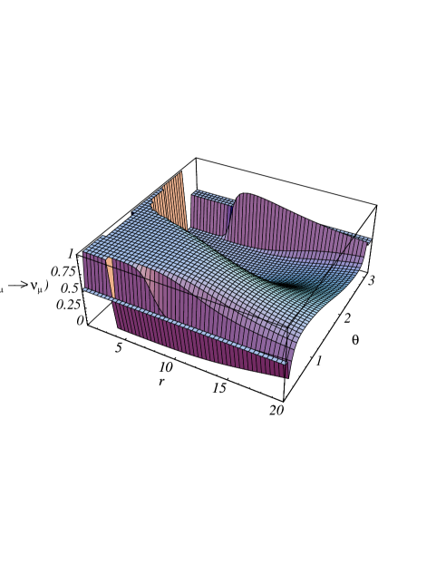
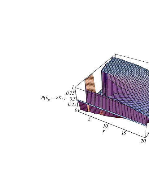
FIG. 4.: Plot of the persistence (left) and transition (right) probabilities as functions of $(r,\theta)$ for $\mu_{t}=10^{-17}\mu_{B}$, $j=0.15$, $k=0.4$, $a/r_{g}=0.4$, $E=1{\rm PeV}$, $\Delta m^{2}=10^{-8}{\rm eV}^{2}$ and $M=10^{8}M_{\odot}$.

The region in parameter space where adiabatic resonances occur is restricted by $\mu_{t}>\mu^{\rm res}_{\rm min}$, $\left|p\cdot J_{G}\right|>E\mu_{t}B$ and by $E>E_{R}$ (where $E_{R}$ is the resonant energy corresponding to $\vartheta_{G}=\pi/4$). Using (17) and (23) these conditions can be re-written as

$$\nu^{2}>{2\delta\over\pi^{2}},\quad f>\nu,\quad f>\delta$$ (28)

where $\delta=r_{g}\Delta m^{2}/4E$ and $\nu=r_{g}\mu_{t}B$.

From (22) we obtain (for the conditions at hand $P_{LZ}\simeq 0$)

$${\nu\over\delta+f}=\sqrt{{P_{t}(1-P_{t})\over\left|P_{t}-{1\over 2}\right|^{2}}}$$ (29)

where $P_{t}=P(\nu_{\mu}\rightarrow\bar{\nu}_{e})$ denotes the transition probability and we have assumed $\vartheta\simeq 0$.

From (28) and (29) it follows that

$$f+\delta>f>\nu=(f+\delta)\sqrt{{P_{t}(1-P_{t})\over\left|P_{t}-{1\over 2}\right|^{2}}}$$ (30)

which required $P_{t}>(2+\sqrt{2})/4$ or $P_{t}<(2-\sqrt{2})/4$; since these expressions are invariant under the replacement $P_{t}\rightarrow 1-P_{t}$ we will assume $P_{t}>(2+\sqrt{2})/4\simeq 0.85$.

For each fixed value of $P_{t}$ the relations above define a region in the $f-\delta-\nu$ space. The quantity $f$ in (28) takes, for the situations under consideration, the values $10^{-4}-1$ depending on the production region, with the larger values associated with regions closer to the black hole horizon, (see Fig. 2). The allowed region in this space for two values of $P_{t}$ are given in Fig. 5; the contour plot of $\nu$ for various values of $\delta$ and $P_{t}$ are presented in Fig. 6 for a specific allowed value of $f$

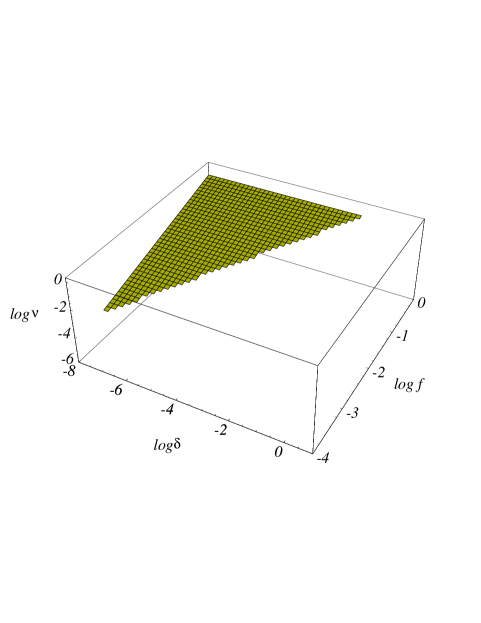
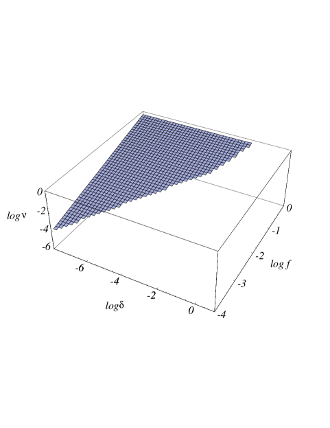
FIG. 5.: Plot of $\nu=r_{g}\mu_{t}B$ as functions of $f$ and $\delta=r_{g}\Delta m^{2}/4E$ for transition probabilities $P_{t}=0.87$ (left) and $P_{t}=0.99$ (right), We used $M=10^{8}M_{\odot}$ and $B=10^{4}$ G and imposed (28).

FIG. 6.: Plot of $\nu=r_{g}\mu_{t}B$ as a function of $\delta=r_{g}\Delta m^{2}/4E$ for various values of the transition probability $P_{t}$; we chose $M=10^{8}M_{\odot}$, B $=10^{4}$ G, $f=10^{-3}$ and imposed (28).

As can be seen clearly from Fig. 6, for a reasonable value of $f$ ($10^{-3}$), adiabatic resonant transitions occur for $\mu_{t}$ in the range $\sim 10^{-18}-10^{-17}\mu_{B}$.

The neutrinos will experience coherent precession if the conditions $\nu>f$ and $\nu>4\delta$ are satisfied; in this case the transition and persistence probabilities are $\sim 1/2$. For example, if $f=10^{-3}$, coherent precession will occur fod $\mu_{t}>10^{-17}\mu_{B}$ (for the above values of $B$ and $r_{g}$) assuming that $\Delta m^{2}<4E\;\mu_{t}\;B$. For sufficiently large values of magnetic moment coherent precession will be the dominant mechanism.

IV Flux Modification due to Gravitational Oscillations.

According to the spherical accretion model [6] high energy neutrinos are produced by proton acceleration at the shock. Such acceleration is assumed to occur by the first order Fermi mechanism resulting in an $E^{-2}$ spectrum extending up to $E^{p}_{max}$. Estimates of expected neutrino fluxes from individual AGN are normalized, using this model, to their observed X-ray luminosities ; the position of the maximum neutrino energy, however, is uncertain because it depends upon the parameters of the particular source. According to the model we have used [16], the neutrino flux at comparatively lower energies is strongly related to the X-ray flux; above 100 TeV the flux depends strongly on the turnover in the primary photon spectrum and one then needs to know the maximum proton energy $E^{p}_{max}$. The results of calculations of Szabo and Protheroe [16] give an approximate formula for the muon neutrino $(\nu_{\mu}+{\bar{\nu}}_{\mu})$ flux in terms of $F_{x}$, the X-ray flux, and $E^{p}_{max}$

$$F_{\nu}\sim 0.25F_{x}\exp(-20E/E^{p}_{max})E^{-2}$$ (31)

where $F_{x}$ is a typical 2-10 Kev X-ray flux in ${\rm erg}\;{\rm cm}^{-2}{\rm s}^{-1}$ and $E$ is the neutrino energy; the flux is plotted in (Fig. 7).

FIG. 7.: Plot of the $(\nu_{\mu}+{\bar{\nu}}_{\mu})$ (solid) and $(\nu_{e}+{\bar{\nu}}_{e})$ (dashed) fluxes, as given by (31), as function of energy E when the X-ray flux equals $F_{x}=10^{-11}{\rm erg}{\rm cm}^{-2}{\rm sec}^{-1}$. $E^{p}_{max}=10^{17}eV$ for AGN luminosity $10^{45}$ ergs/sec, and $\nu_{\mu}:\nu_{e}::2:1$.

Taking $F_{x}$ for a typical AGN to be $10^{-11}\,{\rm erg}{\rm cm}^{-2}{\rm sec}^{-1}$ (corresponding to for 3C273) and $E^{p}_{max}=10^{17}eV$ for an AGN luminosity  $L=10^{45}{\rm ergs}/{\rm sec}$, the resulting neutrino flux is plotted in figure 5.

As discussed in [17] and [18], the detectors AMANDA, Baikal and Nestor are sensitive to a wide range of neutrino parameters and will be able to test a variety of models of neutrino production in the AGN. For neutrino energies above 1 TeV, measuring the ultra high energy muon flux permits an estimation of the $\nu_{\mu}+\bar{\nu}_{\mu}$ flux, for neutrino energies above 3 PeV there is significant contribution to the muon rate due to $\nu_{e}$ interaction with electrons due to the W-resonance effect. Also, as shown in [18], the $\tau$ rate from double bang events can be used to measure the $\nu_{\tau}+\bar{\nu}_{\tau}$ flux at energies 1 PeV and beyond.

We noted earlier that matter effects are negligible in the AGN environment, but that gravity-induced resonances could cause a modification of the neutrino flux of any given flavor. This effect could cause an oscillation to $\tau$ neutrinos   generating a significant flux of $\tau$ neutrinos to which planned experiments will be sensitive in the PeV range [18]. The observed $\tau$ neutrinos would arise due to gravitationally induced resonance oscillations at the AGN itself.

For the case of two flavors $\alpha$ and $\beta$ the observed neutrino flux for species $\alpha$, $F_{\alpha}$, can be expressed in terms of the initially produced neutrino fluxes $F_{\alpha}^{0}$ and $F_{\beta}^{0}$ as

$$F_{\alpha}=[1-P(\nu_{\alpha}\rightarrow\nu_{\beta})]F_{\alpha}^{0}+P(\nu_{\beta}\rightarrow\nu_{\alpha})\,F_{\beta}^{0}$$ (32)

In order to calculate the fluxes in terms of neutrino oscillations we have made a number of simplifying but reasonable assumptions.

• The initial (production) fluxes are assumed to be in the ratio $\nu_{\mu}:\nu_{e}:\nu_{\tau}::2:1:0$. If charged and neutral pions are produced in equal proportions simple counting leads to equal fluxes of $\nu_{\mu}+{\bar{\nu}}_{\mu}$ and photons. The flux of $\nu_{e}+{\bar{\nu}}_{e}$ equals half the flux of $\nu_{\mu}+{\bar{\nu}}_{\mu}$. Ref. [17] discusses the various models AGN neutrino fluxes.

• There are equal numbers of neutrinos and antineutrinos.

• As discussed above and in  [3] matter effects are ignored. Resonances occur through the interaction of gravitational and electromagnetic interactions (proportional to the transition magnetic moment). We concentrate on the case where resonances are present corresponding to small magnetic moments.

• It is assumed that there is no large matter effects in the path from AGN to the earth, so MSW effect does not cause oscillation for neutrinos in transit either. Vacuum oscillations do occur for exceedingly small $\Delta m^{2}$ (for a distance of $\sim 100$ Mpc and energy 1 TeV, $\Delta m^{2}<10^{-19}{\rm eV}^{2}$). Also the intergalactic magnetic field $(\sim 10^{-6}{\rm G})$ may cause spin transitions, but this is again a small effects in the parameter range we consider.

Under these circumstances gravitationally induced spin flavor oscillations are the only important process which could cause neutrino transitions resulting in a modification of the observed fluxes. Figures 8 show the decrease of $\mu$ neutrino flux and the corresponding increase in the $\tau$ neutrino flux produced by resonant oscillations of $\mu$ neutrinos to $\tau$ neutrinos; the effect increases with energy and is very effective in the PeV range where $\tau$ neutrinos can be detected relatively easily.

FIG. 8.: Flux modification of $\mu$ neutrino (left) and $\tau$ neutrino fluxes due to gravitational oscillations of the $\nu_{\mu}-\nu_{\tau}$ system in AGN environment. $\Delta m^{2}=10^{-8}{\rm eV}^{2}$, $\mu_{t}=10^{-17}\mu_{B}$, $r/r_{g}=6$, $\theta=\pi/2$, $j=0.15$, $k=0.4$, $a/r_{g}=0.4$ and $M=10^{8}M_{\odot}$.

The choice of $\mu_{t}=10^{-17}\mu_{B}$ and $\Delta m^{2}=10^{-8}\rm eV^{2}$ for energy 1 PeV falls into the allowed region for gravitational resonant oscillations (Fig. 5) satisfying conditions (28).

V Conclusions

We found that ultra-high energy Majorana neutrinos emanating from AGN are strongly affected by gravitational and electromagnetic effects. For typical values of gravitational current ($J_{G}$), which depends on the allowed black hole and geodesic parameters, gravitational resonant oscillations are found to occur for energies in which future neutrino telescopes [18] will be sensitive provided $\mu_{t}<10^{-17}\mu_{B}$. This therefore causes a significant increase of the corresponding $\tau$ neutrino flux. Gravitational resonant oscillations cause flavor/spin oscillation of such neutrinos where the transition neutrino magnetic moments are small (Fig. 5). For larger magnetic moments, ($\mu_{t}>10^{-17}\mu_{B}$) coherent precession will dominate provided $\Delta m^{2}<E\>\mu_{t}B$ . The increase in the $\tau$ neutrino flux is, of course, accompanied by a corresponding decrease in the $\mu$ neutrino flux. The two cases discussed above can in principle be differentiated by comparing the $\tau$ and $\mu$ neutrino fluxes which would be equal for the case of coherent precession but markedly different for the case of resonant oscillations (Fig. 7 ). However, transition efficiency is greatest for the minimum value of the magnetic moment which corresponds to gravitational resonant oscillations.

We have restricted our calculations to the two neutrino flavor case. A complete study should include at least three flavors and possibly four (to consider the possibility of sterile neutrinos). In the case of solar neutrinos the presence of more flavors can significantly alter the predicted fluxes [13]. However for the present situation where the experimental information on the AGN neutrino flux is quite limited, it is sufficient to determine the various effects and their strengths by using a a two flavor mixing description as we have done in our analysis.

VI Acknowledgements

M.R. would like to thank Prof. Sandip Pakvasa for useful suggestions. This work was supported in part by the US Department of Energy under contract FDP-FG03-94ER40837.

REFERENCES

- [1] See for example G.K. Leontaris and J.D. Vergados, Phys. Lett. B188, 455 (1987); A.Bottino, et. al., Phys. Rev. D34, 862 (1986); S.M.Barr, Phys. Rev. D24, 1895 (1981).
- [2] R.J. Wilkes, in Proc. Slac. Summer Institute 1994 edited by Jennifer Chan and Lilian De Porcel; H.W. Sobel, Nucl. Phys. B (Proc Suppl) 19, 444 (1991); S. Barwick et. al., J. Phys. G: Nucl. Part. Phys. 18, 225 (1992); A. Roberts, Rev. Mod. Phys. 64, 259 (1992); F.Halzen, Nucl. Phys. B S38, 472 (1995).
- [3] D.Piriz, M. Roy and J. Wudka, Phys. Rev. D54, 1587 (1996).
- [4] B. Kayser and A. Goldhaber, Phys. Rev. D28, 2341 (1983); J.F. Nieves, Phys. Rev. D26, 3152 (1982); J.Schechter and J.W.F. Valle, Phys. Rev. D24, 1883 (1981).
- [5] A.Acker, et. al., Phys. Rev. D49, 328 (1994); G.L. Folgi, et. al., Astroparticle Physics 4, 177 (1995).
- [6] R.J. Protheroe and D. Kazanas, Ap. J. 265, 620 (1983); D. Kazanas and D.C. Ellison, Ap. J. 304, 178 (1986).
- [7] A.P. Szabo and R.J. Protheroe, Astroparticle Physics, 2, 375 (1994).
- [8] M.C. Begelman et. al., Rev. Mod. Phys. 56, 255 (1984).
- [9] B. Sakita and R. Tsani, in Rationale of Beings, Fetschrift in honor of G.Takada, edited by K.Ishikawa et. al. (World Scientific, Singapore, 1985), pp 283-290.
- [10] C.S. Lim, W.J. Marciano, Phys. Rev. D37, 1368 (1988).
- [11] L.D.Landau and E.M.Lifshitz, Classical Theory of Fields, 4th edition (Oxford, New York, 1975).
- [12] S.J.Parke, Phys. Rev. Lett. 57, 1275 (1986)
- [13] T.K. Kuo and J.Pantaleone, Rev. Mod. Phys. 61, 937 (1989).
- [14] L.B. Okun, Yad. Fiz. 44, 847 (1986) [Sov. J. Nucl. Phys. 44, 546 (1986)]; L.B. Okun, M.B. Voloshin and M.I. Vyotsky, ibid. 91, 754 (1986) [ibid. 44, 440 (1986)].
- [15] F.W.Stecker and M.H.Salamon, Space Science Reviews 75, 341 (1996 ); A.P. Szabo and R.J. Protheroe, Astro. Phys. 2, 375 (1994); T.K. Gaisser et. al., Phys. Rep. 258, 174 (1995).
- [16] A.P. Szabo and R.J. Protheroe, in High Energy Neutrino Astrophysics, Proceedings of the workshop, Honolulu, Hawaii, 1992, edited by V.J. Stenger et. al. (World Scientific, Singapore,1992). R.J. Protheroe and T.Stanev, ibid.
- [17] R. Gandhi, et. al., hep-ph/9604276 (unpublished), report number AZPH-TH-96-12.
- [18] J.G . Learned and S.Pakvasa, Astroparticle Physics, 3, 267 (1995).