hep-ph/9703286 CERN-TH/96-369
bla DFPD 96/TH/68

Aspects of spontaneously broken $N=1$ global supersymmetry in the presence of gauge interactions

Andrea Brignole

Theory Division, CERN, CH-1211 Geneva 23, Switzerland

Ferruccio Feruglio

Dipartimento di Fisica, Università di Padova, I-35131 Padua, Italy

and

Fabio Zwirner

INFN, Sezione di Padova, I-35131 Padua, Italy

We discuss models where $N=1$ global supersymmetry is spontaneously broken, at the classical level, in the presence of non-anomalous gauge interactions. We take such models as effective theories, valid up to some suitable scale and arising from supergravity models with a light gravitino, and therefore we allow them to contain non-renormalizable interactions. First, we examine the case where the goldstino is a gauge singlet. We elucidate the model-independent relations between supersymmetry-breaking masses and some associated interactions, with special attention to the behaviour of some four-particle scattering amplitudes in the high- and low-energy limits. The former gives constraints from tree-level unitarity, the latter affects the phenomenological lower bounds on the gravitino mass. In particular, we give new results for the annihilation of photons into gravitinos, and discuss their implications. We then examine the case with no neutral chiral superfields, so that the goldstino is charged, and the gauge symmetry is also broken. In this context, we discuss the singularity structure and the associated unitarity constraints, relating the scales of supersymmetry and gauge symmetry breaking. We conclude by commenting on possible realistic examples, where the broken gauge symmetry is associated with grand or electroweak unification.

CERN-TH/96-369
December 1996

1 Introduction

According to the present theoretical wisdom, space-time supersymmetry is likely to play a rôle in the unification of all fundamental interactions, including gravity, and in the resolution of the naturalness problem of the Standard Model (for reviews and references, see e.g. [1]). The major obstacle to the construction of a predictive supersymmetric extension of the Standard Model is our limited understanding of the physics underlying the spontaneous breaking of supersymmetry. However, the general ‘kinematical’ aspects of the problem are well understood [2, 3]. If ${\Lambda}_{S}$ is the scale of supersymmetry breaking, the mass splittings in the different sectors of the model are given by $\Delta m^{2}\sim\lambda\,{\Lambda}_{S}^{2}$, where $\lambda$ is the effective coupling of the goldstino supermultiplet (whose fermionic degrees of freedom provide the $\pm 1/2$ helicity components of the massive spin-$3/2$ gravitino) to the sector under consideration. Even assuming a given size for the mass splittings (for example, the electroweak scale), this leaves an ambiguity in the size of ${\Lambda}_{S}$. If ${\Lambda}_{S}^{4}<\Delta m^{2}\,M_{\rm P}^{2}$, where $M_{\rm P}\equiv(8\pi G_{N})^{-1/2}\simeq 2.4\times 10^{18}{\rm\;GeV}$ is the (reduced) Planck mass, the effective couplings of the goldstino supermultiplet to the other chiral and vector supermultiplets are stronger than the gravitational ones. Therefore, for most practical purposes, we can discuss spontaneous supersymmetry breaking in an effective non-renormalizable theory with global supersymmetry: formally, we can start from the general supergravity formalism [4] and take the limit $M_{\rm P}\to\infty$, while keeping ${\Lambda}_{S}$ constant [5]. We just need to recall that in the physical spectrum there is a gravitino of mass $m_{3/2}=\Lambda_{S}^{2}/(\sqrt{3}M_{\rm P})$, whose interactions at energies $E\gg m_{3/2}$ are well approximated, thanks to an equivalence theorem [6], by those of the massless goldstino in the global limit. On physical grounds, models with a relatively low scale of supersymmetry breaking may be favoured by arguments related with cosmology and with the flavour problem, which explains their recent revival [7].

In the study of low-energy supersymmetry breaking, two different and complementary approaches can be followed. The ‘microscopic’ approach tries to understand the symmetries and the dynamics that may generate the scales ${\Lambda}_{S}$ and $\Delta m^{2}$ at the level of the fundamental theory. The ‘macroscopic’ approach tries to write down an effective theory, valid in a suitable energy range, where the underlying dynamics is encoded in a set of non-renormalizable interactions, and the spontaneous breaking of supersymmetry is described at the classical level. Intermediate approaches are possible [7], but we will not discuss them here. The ‘macroscopic’ approach has a limited predictive power, but may be useful to parametrize the model-independent features of the resulting phenomenology, modding out the dependence on the presently unknown aspects of the fundamental theory. In this paper, we adopt such an approach, with the purpose of discussing some aspects of spontaneous supersymmetry breaking in the presence of gauge interactions.

In section 2, we examine the case where the goldstino is a gauge singlet and the gauge symmetry remains unbroken. As an illustrative example, we study a class of models with gauge group $U(1)$ and two neutral chiral superfields, $S$ and $A$, which is sufficient to understand most qualitative aspects of the general case. In particular, we consider the model-independent relations between various supersymmetry-breaking masses and some associated interactions. Many results of this section are not new, but we try to give a simple and systematic presentation, avoiding the unnecessary use of the supergravity formalism, and stressing the general cancellation mechanisms that control the low- and high-energy behaviour of some four-particle scattering amplitudes. In the low-energy limit, we extract some useful information on the phenomenology of a superlight gravitino within realistic models. In particular, we clarify the structure of the low-energy interactions between photons and gravitinos, which was used in the past [8, 9, 10] to establish lower bounds on the gravitino mass, via the rôle played by processes such as photon–photon annihilation into gravitino pairs (or vice versa) in cosmological nucleosynthesis or in the evolution of supernovae. To do so, we generalize previous calculations of the relevant scattering amplitudes and cross-sections. In the high-energy limit, we use tree-level unitarity to put an upper bound on the energy range of validity of the effective theory, as a function of the particle masses and of the scale of supersymmetry breaking. We conclude the section with simple examples of explicit models.

In section 3, we examine models that do not contain neutral superfields, so that the gauge symmetry must be broken simultaneously with supersymmetry. We construct a minimal example, with gauge group $U(1)$ and two chiral superfields $(H_{1},H_{2})$ of opposite charges, which allows us to discuss in simple terms a number of general properties of possible physical relevance. We show that, in order to have a supersymmetry-breaking vacuum, either the superpotential or the Kähler metric must be singular at the origin, so that the configurations with unbroken gauge group are excluded from the space of allowed background field values. Considering first the simple case of canonical kinetic terms, we show that the unique choice of superpotential leading to a supersymmetry-breaking classical vacuum has a conical singularity at the origin, $w={\Lambda}_{S}^{2}\sqrt{2H_{1}H_{2}}$ (apart from irrelevant constant terms and redefinitions of ${\Lambda}_{S}$). We also show how this model can be obtained from a supergravity model with vanishing vacuum energy, previously studied in ref. [11], by taking the appropriate flat limit. We then discuss how the scales ${\Lambda}_{S}$ and $v$, associated with supersymmetry and gauge symmetry breaking, respectively, control the spectrum and the interactions, and show that ${\Lambda}_{S}\gg v$ would lead to a premature violation of tree-level unitarity and correspond to a strong coupling régime. We continue by extending the treatment to the case of non-canonical kinetic terms, with the formulation of an explicit example of this sort. We conclude by generalizing our results to a much wider class of models, and commenting on possible realistic applications, where supersymmetry breaking is associated with the breaking of either a grand-unified symmetry or the electroweak symmetry.

Some notational and calculational details are confined to the appendix, which contains the explicit form of an $N=1$ globally supersymmetric effective Lagrangian, in the simple case where the gauge group is a non-anomalous $U(1)$ and there is no Fayet–Iliopoulos term, as well as the corresponding expression for the scalar potential in the locally supersymmetric case.

2 The case of a singlet goldstino

As anticipated in the introduction, we will examine in this section, in an effective theory approach, some model-independent features of $N=1$ globally supersymmetric gauge theories coupled to matter, with spontaneously broken supersymmetry and the goldstino transforming as a gauge singlet. Our aim is to make explicit some relations, associated with low-energy theorems [12], between supersymmetry-breaking masses and certain cubic and quartic interactions involving the goldstino and/or its spin-0 superpartners. These interactions in turn control the low- and high-energy behaviour of some four-particle scattering amplitudes, which can be used to establish lower bounds on the scale of supersymmetry breaking (and therefore on the gravitino mass) and to constrain the range of validity of the effective theory in energy and parameter space.

For our purpose, it will be sufficient to consider a class of $N=1$ globally supersymmetric models with gauge group $G=U(1)$ and two neutral chiral superfields, with physical components $(S,{\tilde{S}})$ and $(A,{\tilde{A}})$. We anticipate that the two chiral superfields will play quite different rôles in the following. The $S$-multiplet will be directly responsible for supersymmetry breaking and will contain the goldstino. Indeed, most of the considerations of the present section do not require the presence of the $A$-multiplet. We introduce it here for two reasons: first, to develop a formalism that can be easily adapted to the generalization presented in the next section; second, because $A$ mimics the rôle of matter superfields in realistic models. We recall that the most general effective Lagrangian with the above field content is determined by a superpotential $w$, a Kähler potential $K$ and a gauge kinetic function $f$. Incidentally, notice that, since the chiral superfields are neutral, the gauge kinetic function is the only source of interactions between vector and chiral multiplets. Having in mind the different rôles to be played by $S$ and $A$, we will retain the full $S$-field dependence of the basic functions $w,K,f$ and consider only a power expansion in the $A$ field. More precisely, we will assume the following functional forms:

$$w = {\hat{w}}(S)+{1\over 2}{\tilde{w}}(S)A^{2}+\ldots\,,$$ (2.1)

$$K = {\hat{K}}(S,\overline{S})+{\tilde{K}}(S,\overline{S})|A|^{2}+{1\over 2}[{\tilde{H}}(S,\overline{S})A^{2}+{\rm h.c.}]+\ldots\,,$$ (2.2)

$$f = {\hat{f}}(S)+{1\over 2}{\tilde{f}}(S)A^{2}+\ldots\,,$$ (2.3)

where the dots stand for higher-order terms in $A$. Since there are no charged fields, the classical potential $V$ is just $||F||^{2}=w_{i}(K^{-1})^{i\,{\overline{\j}}}{\overline{w}}_{\overline{\j}}$, as in eq. (A.11). We assume that $w$ and $K$ are such that, at the minimum of $V$:

$$\langle F^{S}\rangle\neq 0\,,\;\;\;\;\;\langle F^{A}\rangle=0\,,\;\;\;\;\;\langle A\rangle=0\,,$$ (2.4)

whereas we do not need to specify whether $\langle S\rangle$ is vanishing or not. Also, the fact that $\langle A\rangle=0$ and $\langle F^{A}\rangle=0$ are at least local extrema is already a consequence of eqs. (2.1) and (2.2). Indeed, only the assumption that $\langle F^{S}\rangle\neq 0$ is restrictive, since it amounts to requiring that supersymmetry be spontaneously broken. For the purposes of this section, however, we do not need to commit ourselves to a specific choice of ${\hat{w}}(S)$ and ${\hat{K}}(S,\overline{S})$ that realizes such a situation.

2.1 The spectrum

We begin the study of our class of models by discussing the general features of the mass spectrum. Starting with the supersymmetry-breaking sector, we can identify the goldstino with the fermion $\tilde{S}$: $m_{\tilde{S}}=0$. We can verify this with the help of eq. (A.17) and of the minimization condition for the scalar potential along the $S$ direction:

$$\langle(\log{\hat{w}}_{S})_{S}-(\log{\hat{K}}_{{\overline{S}}S})_{S}\rangle=0\,.$$ (2.5)

Decomposing the shifted $S$ field into real and imaginary parts,

$$S\equiv\langle S\rangle+{\varphi_{S}+i\varphi^{\prime}_{S}\over\sqrt{2}}\,,$$ (2.6)

and assuming for simplicity that $\langle V_{SS}\rangle=\langle V_{\overline{S}\overline{S}}\rangle$ (the generalization is straightforward), $\varphi_{S}$ and $\varphi_{S^{\prime}}$ are mass eigenstates, with eigenvalues

$$m^{2}_{S} = \langle|F^{S}|^{2}[-(\log{\hat{K}}_{{\overline{S}}S})_{{\overline{S}}S}-(\log{\hat{K}}_{{\overline{S}}S})_{SS}+(\log{\hat{w}}_{S})_{SS}]\rangle\,,$$

$$m^{2}_{S^{\prime}} = \langle|F^{S}|^{2}[-(\log{\hat{K}}_{{\overline{S}}S})_{{\overline{S}}S}+(\log{\hat{K}}_{{\overline{S}}S})_{SS}-(\log{\hat{w}}_{S})_{SS}]\rangle\,,$$ (2.7)

where $F^{S}=(K^{-1})^{S\overline{\j}}\overline{w}_{\overline{\j}}$. The sum of the squared scalar masses in the $S$-sector has a geometrical meaning [13], and is given by

$$m^{2}_{S}+m^{2}_{S^{\prime}}=2\langle|F^{S}|^{2}[-(\log{\hat{K}}_{{\overline{S}}S})_{{\overline{S}}S}]\rangle=-2\left\langle|F^{S}|^{2}{R_{S{\overline{S}}S{\overline{S}}}\over{\hat{K}}_{{\overline{S}}S}}\right\rangle\,,$$ (2.8)

where $R_{S\overline{S}S\overline{S}}\equiv{\hat{K}}_{S\overline{S}S\overline{S}}-|{\hat{K}}_{\overline{S}SS}|^{2}/{\hat{K}}_{\overline{S}S}$ is the curvature of the Kähler manifold for the complex field $S$. Notice that, in order to have a stable minimum in the $S$ direction, one needs $m_{S}^{2}+m_{S^{\prime}}^{2}>0$, therefore $R_{S\overline{S}S\overline{S}}<0$. This can be contrasted with hidden sector breaking in supergravity models, where one usually deals with manifolds of positive curvature, so that curvature contributions to scalar squared masses are negative. In such a case, however, positivity can be rescued by an additional non-negligible positive contribution to scalar squared masses coming from gravitational interactions and proportional to the gravitino mass.

Moving to the gauge sector, the $U(1)$ gauge boson is massless, since the gauge symmetry is unbroken: $m_{V}=0$. The gaugino is a mass eigenstate, with mass scaling with $F^{S}$ and controlled by the derivative of ${\hat{f}}$:

$$M={1\over 2}\left\langle{{\hat{f}}_{S}F^{S}\over{\rm Re\,}{\hat{f}}}\right\rangle\,.$$ (2.9)

We recall that gaugino masses have expressions of this type also in supergravity models.

Notice that, if the kinetic terms were canonical, there would be no supersymmetry-breaking mass splittings in the $S$ and in the gauge sectors. This is a consequence of a general result of global supersymmetry [13], which can be conveniently described in terms of ${\rm Str\;}{\cal M}^{2}\equiv\sum_{i}(-1)^{2J_{i}}(2J_{i}+1)m_{i}^{2}$, where $m_{i}$ and $J_{i}$ are mass and spin of the i-th physical state: for canonical kinetic terms and in the absence of anomalous $U(1)$ gauge factors, ${\rm Str\;}{\cal M}^{2}\equiv 0$ in each separate sector of the mass spectrum. In the $(S,\tilde{S})$ sector, which contains the massless goldstino, no mass splitting would be allowed. In the $(\lambda,A_{\mu})$ sector, which contains a massless gauge boson, the gaugino would also be massless. As we have seen, this trivial pattern is changed by the introduction of non-canonical kinetic terms.

Non-canonical kinetic terms play an important rôle also in the spectrum of the $A$ sector. Here the fermion mass is

$$m_{\tilde{A}}=\langle{\tilde{K}}^{-1}({\tilde{w}}-\overline{F}^{\overline{S}}{\tilde{H}}_{\overline{S}})\rangle\,.$$ (2.10)

The elements of the spin-0 mass matrix are, in obvious notation:

$$m^{2}_{A\overline{A}}=|m_{\tilde{A}}|^{2}+\tilde{m}^{2}_{A}\,,$$ (2.11)

where

$$\tilde{m}^{2}_{A}=\langle\overline{F}^{\overline{S}}(-\log{\tilde{K}})_{\overline{S}S}F^{S}\rangle\,,$$ (2.12)

and

$$m^{2}_{AA}=\left\langle[{\tilde{K}}^{-1}{\tilde{w}}]\left[\left(\log{{\tilde{w}}\over{\tilde{K}}^{2}}\right)_{S}F^{S}\right]+[-{\tilde{K}}^{-1}\overline{F}^{\overline{S}}{\tilde{H}}_{\overline{S}}]\left[\left(\log{{\tilde{H}}_{\overline{S}}\over{\tilde{K}}^{2}}\right)_{S}F^{S}\right]\right\rangle\,.$$ (2.13)

Under the simplifying assumption that $m^{2}_{AA}$ is real (the generalization is straightforward), the real and imaginary parts of the field $A$,

$$A\equiv{\varphi_{A}+i\varphi^{\prime}_{A}\over\sqrt{2}}\,,$$ (2.14)

are mass eigenstates, and the corresponding eigenvalues are

$$m_{A}^{2}=m_{A\overline{A}}^{2}+m^{2}_{AA}\,,\;\;\;\;\;m_{A^{\prime}}^{2}=m_{A\overline{A}}^{2}-m^{2}_{AA}\,.$$ (2.15)

Notice that also the masses of the $A$ sector have some formal similarity with those derived in supergravity models. The fermion mass $m_{\tilde{A}}$ is the sum of two pieces (‘generalized $\mu$ parameters’), one coming directly from the superpotential, the other induced from the Kähler potential and scaling with $F^{S}$. The diagonal scalar mass $m^{2}_{A\overline{A}}$ is the sum of the squared fermion mass and an additional contribution $\tilde{m}^{2}_{A}$ (‘diagonal soft mass’), scaling with $|F^{S}|^{2}$ and controlled by the curvature of the $S$–$A$ Kähler manifold. The off-diagonal scalar mass $m^{2}_{AA}$ is the sum of two pieces, proportional to the corresponding pieces composing the fermion mass, with proportionality factors scaling with $F^{S}$ (‘generalized $B$ parameters’).

2.2 Cubic interactions

The non-canonical forms of $K$ and $f$, which are at the origin of the supersymmetry-breaking mass splittings in the various sectors, also generate non-trivial interactions, which we will now discuss in a systematic way, applying the general formulae of the appendix. Here and in the following, when writing down interaction terms derived from expansions around a given vacuum, we will work with canonically normalized fields, without introducing a different symbol to denote them. We will also introduce the quantity $F\equiv\langle{\overline{w}}_{\overline{S}}(K_{\overline{S}S})^{-1/2}\rangle$, with the property that $|F|^{2}=\langle||F||^{2}\rangle$. Whenever possible, we will try to express the couplings in terms of the physical masses and of the supersymmetry-breaking scale $F$. In this subsection we will focus on cubic interactions and some related decay processes. We will also impose a sort of minimal unitarity (or perturbativity) requirement, by asking that decay widths be not larger than the masses of the decaying particles. This will lead to simple relations where (combinations of) masses are bounded from above by the supersymmetry breaking scale. Also, we anticipate that the cubic couplings studied here play a crucial rôle in building the four-particle amplitudes discussed in the next subsection.

2.2.1 $S\gamma\gamma$

We start by expanding the generalized kinetic terms for the gauge boson, eq. (A.8), which leads to the following cubic couplings involving two photons and the spin-0 components of $S$:

$$-{1\over 2\sqrt{2}}\left[{\rm Re\,}\left(M\over F\right)\varphi_{S}-{\rm Im\,}\left(M\over F\right)\varphi_{S}^{\prime}\right]F_{\mu\nu}F^{\mu\nu}$$ (2.16)

$$+{1\over 4\sqrt{2}}\left[{\rm Im\,}\left(M\over F\right)\varphi_{S}+{\rm Re\,}\left(M\over F\right)\varphi_{S}^{\prime}\right]\epsilon^{\mu\nu\rho\sigma}F_{\mu\nu}F_{\rho\sigma}\,.$$ (2.17)

The physical processes directly controlled by these couplings are the decays $\varphi\rightarrow\gamma\gamma$, where $\varphi$ denotes any of the two fields $\varphi_{S}$ and $\varphi_{S}^{\prime}$, and $\gamma$ denotes the massless gauge boson (‘photon’). The decay rate is easily computed to be:

$$\Gamma(\varphi\to\gamma\gamma)={m_{\varphi}^{3}\over 32\pi}{|M|^{2}\over|F|^{2}}\,;$$ (2.18)

then the requirement $\Gamma_{\varphi}<m_{\varphi}$ translates into the following bound:

$$m_{\varphi}|M|<\sqrt{32\pi}|F|\,.$$ (2.19)

2.2.2 $S\lambda\lambda$

Expanding the gaugino bilinears, eqs. (A.13) and (A.16), and making use of the gaugino equation of motion, we get the following effective Yukawa couplings involving two gauginos and the spin-0 components of $S$:

$${1\over 4\sqrt{2}}\left[-{4M^{2}\over F}+\left\langle{{\hat{f}}_{SS}-{\hat{f}}_{S}\Gamma^{S}_{SS}\over{\rm Re\,}{\hat{f}}\,{\hat{K}}_{\overline{S}S}}\right\rangle F\right](\varphi_{S}+i\varphi_{S}^{\prime})\lambda\lambda+{\rm h.c.}\,,$$ (2.20)

where $\Gamma^{S}_{SS}\equiv(K^{-1})^{S\overline{\i}}K_{\overline{\i}SS}$ and $\langle\Gamma^{S}_{SS}\rangle={\hat{K}}_{\overline{S}SS}/{\hat{K}}_{\overline{S}S}$. Of course, the gauginos appearing in these effective couplings are understood to be external, in a physical process, otherwise the original derivative vertex should be used. A possible application is a decay of the type $\varphi\to\lambda\lambda$, which is kinematically allowed only if $|m_{\varphi}|>2|M|$.

2.2.3 $S\tilde{S}\tilde{S}$

Expanding the bilinears in the goldstino $\tilde{S}$, eqs. (A.15) and (A.17), and making use of the goldstino equation of motion, we get the following effective Yukawa couplings involving two goldstinos and the spin-0 components of $S$, in agreement with [14]:

$$-{1\over 2\sqrt{2}}{m_{S}^{2}\over F}\varphi_{S}\tilde{S}\tilde{S}+{i\over 2\sqrt{2}}{m_{S^{\prime}}^{2}\over F}\varphi_{S}^{\prime}\tilde{S}\tilde{S}+{\rm h.c.}$$ (2.21)

The physical processes directly controlled by these couplings are the decays $\varphi\rightarrow\tilde{S}\tilde{S}$. The decay rate is easily computed to be:

$$\Gamma(\varphi\to\tilde{S}\tilde{S})={m_{\varphi}^{5}\over 32\pi|F|^{2}}\,;$$ (2.22)

then the requirement $\Gamma_{\varphi}<m_{\varphi}$ translates into the following bound:

$$m_{\varphi}^{2}<\sqrt{32\pi}|F|\,.$$ (2.23)

2.2.4 $SSS$

Expanding the scalar potential, eq. (A.10), one can generate cubic couplings in the spin-0 components of $S$, controlled by:

$$\langle V_{\overline{S}SS}\rangle=|F|^{2}\left\langle-\left(\log{\hat{K}}_{\overline{S}S}\right)_{\overline{S}SS}\right\rangle\,,$$ (2.24)

$$\langle V_{SSS}\rangle=|F|^{2}\left\langle-\left(\log{\hat{K}}_{\overline{S}S}\right)_{SSS}+\left(\log{\hat{w}}_{S}\right)_{SSS}\right\rangle\,.$$ (2.25)

As examples of physical processes controlled by the above couplings, one could think of the possible decays $\varphi\to\varphi^{\prime}\varphi^{\prime}$, if they are kinematically allowed.

2.2.5 $\tilde{S}\lambda\gamma$

Expanding the gaugino–goldstino bilinear, eq. (A.14), one generates a cubic photino–goldstino–photon coupling of the form

$$-{1\over\sqrt{2}}\displaystyle{M\over F}\tilde{S}\sigma^{\mu\nu}\lambda F_{\mu\nu}+{\rm h.c.}$$ (2.26)

The physical process directly controlled by this coupling is the decay $\lambda\rightarrow\gamma\tilde{S}$. The decay rate is easily computed to be [15]:

$$\Gamma(\lambda\to\gamma\tilde{S})={|M|^{5}\over 16\pi|F|^{2}}\,;$$ (2.27)

then the requirement $\Gamma_{\lambda}<|M|$ translates into the following bound:

$$|M|^{2}<\sqrt{16\pi}|F|\,.$$ (2.28)

2.2.6 $S\tilde{A}\tilde{A}$, $A\tilde{A}\tilde{S}$

Finally, expanding eqs. (A.15) and (A.17) and using again the fermion equations of motion, we get the following effective Yukawa interactions coupling the $S$-sector to the $A$-sector:

$$-{1\over 2\sqrt{2}}\left\{{m_{A}^{2}-m_{A^{\prime}}^{2}\over 2F}-\langle{({\tilde{H}}_{SS}-{\tilde{H}}_{S}\Gamma^{S}_{SS})^{*}\over{\tilde{K}}{\hat{K}}_{\overline{S}S}}\rangle F^{*}\right\}\varphi_{S}\tilde{A}\tilde{A}+{\rm h.c.}\,,$$ (2.29)

$$+{i\over 2\sqrt{2}}\left\{-{m_{A}^{2}-m_{A^{\prime}}^{2}\over 2F}-\langle{({\tilde{H}}_{SS}-{\tilde{H}}_{S}\Gamma^{S}_{SS})^{*}\over{\tilde{K}}{\hat{K}}_{\overline{S}S}}\rangle F^{*}\right\}\varphi_{S}^{\prime}\tilde{A}\tilde{A}+{\rm h.c.}\,,$$ (2.30)

$$-{m_{A}^{2}-m_{\tilde{A}}^{2}\over\sqrt{2}F}\varphi_{A}\tilde{A}\tilde{S}+i{m_{A^{\prime}}^{2}-m_{\tilde{A}}^{2}\over\sqrt{2}F}\varphi^{\prime}_{A}\tilde{A}\tilde{S}+{\rm h.c.}$$ (2.31)

The latter couplings involving the goldstino are especially simple and are manifestly related to the mass splittings in the $(A,{\tilde{A}})$ multiplet, similarly to the cases considered above. The decay rates for the associated processes $\varphi_{A}\rightarrow{\tilde{A}}{\tilde{S}}$ (or ${\tilde{A}}\rightarrow\varphi_{A}{\tilde{S}}$) and $\varphi^{\prime}_{A}\rightarrow{\tilde{A}}{\tilde{S}}$ (or ${\tilde{A}}\rightarrow\varphi^{\prime}_{A}{\tilde{S}}$) are easily evaluated. The general result for decays of this kind is

$$\Gamma={(\Delta m^{2})^{4}\over 16\pi m^{3}|F|^{2}}\,,$$ (2.32)

where $\Delta m^{2}$ denotes the mass splitting and $m$ the mass of the decaying particle. The requirement $\Gamma<m$ now translates into bounds of the form

$${(\Delta m^{2})^{2}\over m^{2}}<\sqrt{16\pi}|F|\,.$$ (2.33)

In particular, if the final particle produced together with the goldstino is massless, then $\Delta m^{2}=m^{2}$ and the above results simplify to $\Gamma=m^{5}/(16\pi|F|^{2})$ and $m^{2}<\sqrt{16\pi}|F|$, which are the same as (2.27) and (2.28) for gauginos. The analogous relations (2.22) and (2.23) for the scalar partners of the goldstino have an extra factor $1/2$ just because of the identical particles in the final state.

The bounds of eqs. (2.19), (2.23), (2.28) and (2.33) show that the typical supersymmetry-breaking mass splittings should not be larger than a few times the supersymmetry-breaking scale, otherwise some coupling constant would become large and a particle interpretation would become problematic for some of the states explicitly considered here.

2.3 Quartic interactions

We have seen how the presence of non-trivial functions $w$, $K$ and $f$ generates mass terms and cubic interactions. Several quartic and higher interactions are generated as well. For instance, the quartic interactions can involve four bosons, two bosons and two fermions, or four fermions. Instead of discussing all of them, we will mainly focus on four-particle physical amplitudes involving goldstinos, which are more model-independent and exhibit peculiar low- and high-energy properties. Such amplitudes may receive both ‘contact’ contributions, directly from the Lagrangian, and ‘exchange’ contributions, where two cubic interactions are connected by a particle propagator. In the low-energy régime, important cancellations make the amplitudes vanish with energy more rapidly than the individual contributions. This softer behaviour is consistent with the derivative character of the effective goldstino interactions at low energy. In the high-energy régime, the contact terms tend to dominate and make the amplitudes grow until unitarity breaks down. In this régime, the requirement of tree-level unitarity can be used to get upper bounds on the energy itself, i.e. on the validity of the effective theory, as a function of the particle masses and of the supersymmetry breaking scale. Notice that, in the examples discussed below, the source of unitarity violations is the non-canonical character of $K$ and $f$: the relevant contact terms would be absent in the case of canonical kinetic terms. We also recall that, in the framework of an underlying supergravity theory, an equivalence theorem [6] assures that the goldstino components of the gravitino give the leading contribution to gravitino scattering amplitudes when $s\gg m^{2}_{3/2}$. This condition will always be understood in the following, even when we discuss the low-energy régimes $s\ll($masses$)^{2}$. In the high-energy régime, our formalism will lead to considerable simplifications with respect to the full supergravity formalism, since the cancellation mechanisms, implied by the equivalence theorem, will be automatically taken into account from the beginning.

2.3.1 $\tilde{S}\tilde{S}\tilde{S}\tilde{S}$

The simplest amplitudes that exhibit the above properties are those involving four goldstinos, a case already discussed in [14] in connection with the goldstino–gravitino equivalence theorem: the relevant Feynman diagrams are shown schematically in fig. 1.

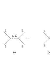
Figure 1: Tree–level Feynman diagrams contributing to the four-goldstino scattering amplitudes: (a) $(\varphi_{S},\varphi_{S}^{\prime})$ exchange (the dots stand for the $t$- and $u$- channel diagrams); (b) contact interactions.

As an illustrative example, let us reconsider the scattering amplitude ${\cal A}={\cal A}({\tilde{S}}_{-}{\tilde{S}}_{-}\rightarrow{\tilde{S}}_{-}{\tilde{S}}_{-})$, involving four left-handed goldstinos ${\tilde{S}}_{-}$. This amplitude receives two contributions from the $s$-channel exchange of the scalars ${\varphi_{S}}$ and ${\varphi_{S}^{\prime}}$ (fig. 1a), which couple to the external goldstinos through the cubic vertices (2.21). In addition, ${\cal A}$ receives a contact contribution (fig. 1b) from the four-fermion Lagrangian term

$$-{1\over 8}{m_{S}^{2}+m_{S^{\prime}}^{2}\over|F|^{2}}\tilde{S}\tilde{S}\overline{\tilde{S}}\overline{\tilde{S}}\,,$$ (2.34)

which originates from eqs. (A.23) and (2.8). The three contributions give

$${\cal A} = {s\over 2|F|^{2}}\left({m_{S}^{4}\over s-m_{S}^{2}}+{m_{S^{\prime}}^{4}\over s-m_{S^{\prime}}^{2}}+(m_{S}^{2}+m_{S^{\prime}}^{2})\right)$$ (2.35)

$$= {s^{2}\over 2|F|^{2}}\left({m_{S}^{2}\over s-m_{S}^{2}}+{m_{S^{\prime}}^{2}\over s-m_{S^{\prime}}^{2}}\right)\,,$$ (2.36)

where an overall $s$ factor is just due to the external spinors. In the low-energy limit ($s\ll m_{S}^{2},m_{S^{\prime}}^{2}$), one can clearly see the cancellation of the leading individual terms, proportional to $sm^{2}/|F|^{2}$. The resulting amplitude $|{\cal A}|=s^{2}/|F|^{2}$ has a softer energy dependence, does not depend on the scalar masses, and gives a cross section $\sigma=s^{3}/(32\pi|F|^{4})$. At high energies ($s>m_{S}^{2},m_{S^{\prime}}^{2}$), on the other hand, the contact term alone dominates and produces an amplitude scaling as $|{\cal A}|\sim sm^{2}/|F|^{2}$, which signals a unitarity breakdown for $s\gg|F|^{2}/m^{2}$. The corresponding cross section grows as $\sigma\sim sm^{4}/|F|^{4}$. An accurate determination of the critical energy can be inferred from the detailed analysis of [14], where all four-goldstino helicity amplitudes were computed and the whole scattering matrix was built. Requiring that the largest eigenvalue of the matrix be smaller than 1 in the high energy régime implies that unitarity is violated beyond the critical energy

$$s_{c}=48\pi\frac{|F|^{2}}{m_{S}^{2}+m_{S^{\prime}}^{2}}\,.$$ (2.37)

Therefore the description provided by the model is not reliable beyond this energy cutoff, and we should require $s_{c}$ to be larger than the scalar masses for consistency reasons. If we impose, for example, $s_{c}>m_{S}^{2}+m_{S^{\prime}}^{2}$ we get the bound

$$m_{S}^{2}+m_{S^{\prime}}^{2}<\sqrt{48\pi}|F|\,,$$ (2.38)

which has the same form as (and is consistent with) the previous bound (2.23).

2.3.2 $\tilde{S}\tilde{S}\gamma\gamma$

Another class of interesting processes consists of those involving two goldstinos and two gauge bosons (‘photons’), i.e. the annihilation processes ${\tilde{S}}{\tilde{S}}\rightarrow\gamma\gamma$ and $\gamma\gamma\rightarrow{\tilde{S}}{\tilde{S}}$, and the scattering process ${\tilde{S}}\gamma\rightarrow{\tilde{S}}\gamma$, described by the Feynman diagrams of fig. 2.

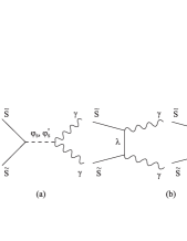
Figure 2: Tree–level Feynman diagrams contributing to the scattering amplitudes with two photons and two goldstinos, for example $\tilde{S}\tilde{S}\to\gamma\gamma$: (a) $(\varphi_{S},\varphi_{S}^{\prime})$ exchange; (b) gaugino exchange.

The Lagrangian does not contain any contact term contributing to these processes. On the other hand, one has to take into account contributions from virtual ${\varphi_{S}},{\varphi_{S}^{\prime}}$ exchange (fig. 2a), controlled by the cubic couplings (2.16), (2.17), (2.21), and virtual gaugino exchange (fig. 2b), controlled by the cubic coupling (2.26). We first consider the low-energy régime ($s\ll m_{S}^{2},m_{S^{\prime}}^{2},|M|^{2}$), where again the full amplitudes are softer than the individual contributions, owing to a crucial cancellation. A straightforward way to check such a cancellation consists in integrating out the massive fields from the Lagrangian and looking at the leading effective Lagrangian terms coupling two goldstinos and two gauge bosons. Integrating out the scalars leads to an effective term

$${M\over 8F^{2}}\left(F_{\mu\nu}F^{\mu\nu}+{i\over 2}\epsilon^{\mu\nu\rho\sigma}F_{\mu\nu}F_{\rho\sigma}\right){\tilde{S}}{\tilde{S}}+{\rm h.c.}\,,$$ (2.39)

which gives contributions $\sim E^{3}M/F^{2}$ to the amplitudes, whereas integrating out the gauginos leads to an identical effective term with opposite sign. Therefore the amplitudes do not receive any net contribution proportional to $E^{3}$. The next term in the expansion couples ${\tilde{S}}$ to ${\overline{\tilde{S}}}$ and contains an extra derivative, coming from the gaugino propagator:

$$-{i\over 2|F|^{2}}F_{\mu\nu}{\overline{\tilde{S}}}{\overline{\sigma}}^{\mu\nu}{\overline{\sigma}}^{\tau}\sigma^{\rho\sigma}\partial_{\tau}(\tilde{S}F_{\rho\sigma})=-{i\over 2|F|^{2}}F_{\mu\nu}F^{\mu}_{\;\;\tau}\left[{\overline{\tilde{S}}}{\overline{\sigma}}^{\nu}\partial^{\tau}{\tilde{S}}-(\partial^{\tau}{\overline{\tilde{S}}}){\overline{\sigma}}^{\nu}{\tilde{S}}\right]\,,$$ (2.40)

where the equations of motion for the goldstino and the photon have been used in the second step. The amplitudes corresponding to the above effective operator are proportional to $E^{4}/|F|^{2}$ and do not depend on masses. This behaviour is analogous to the one of the four-goldstino amplitude discussed above and leads to cross sections scaling again as $\sigma\sim s^{3}/|F|^{4}$. The important cancellation explained above was not accounted for by the recent calculation of ref. [9], where a result $\sigma\sim s^{2}|M|^{2}/|F|^{4}$ was obtained for the annihilation process ${\tilde{S}}{\tilde{S}}\rightarrow\gamma\gamma$. Indeed, existing calculations are only valid either in the high-energy régime [16] or in the massless limit for the spin-0 partners of the goldstino [17, 9]. More details and a discussion of the phenomenological implications of our results will be given in section 2.4. We now consider the above processes in the high-energy régime ($s>m_{S}^{2},m_{S^{\prime}}^{2},|M|^{2}$), where unitarity violations are expected. Here the most dangerous amplitudes correspond to external ${\tilde{S}}$, ${\overline{\tilde{S}}}$ and are dominated by gaugino exchange. They grow as $E^{2}|M|^{2}/|F|^{2}$, which signals a unitarity breakdown for $s\gg|F|^{2}/|M|^{2}$. The corresponding cross sections grow as $\sigma\sim s|M|^{4}/|F|^{4}$. Imposing the consistency condition that the critical energy be larger than $|M|$ leads to a bound of the same form as the previous bound (2.28), $|M|^{2}<{\cal O}(10)|F|$. Similarly, imposing the consistency condition that the critical energy be larger than $m_{\varphi}$, where $\varphi$ is now the heavier of $\varphi_{S}$ and $\varphi_{S^{\prime}}$, leads to a bound of the same form as the previous bound (2.19), $|m_{\varphi}M|<{\cal O}(10)|F|$. Both bounds are in agreement with the supergravity results of ref. [17].

2.3.3 $\tilde{S}\tilde{S}\lambda\lambda$

We now move to processes involving two goldstinos and two gauginos, i.e. $\tilde{S}\tilde{S}\to\lambda\lambda$, $\lambda\lambda\to\tilde{S}\tilde{S}$ and $\tilde{S}\lambda\to\tilde{S}\lambda$, described by the Feynman diagrams of fig. 3.

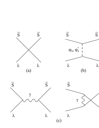
Figure 3: Tree–level Feynman diagrams contributing to the goldstino-gaugino scattering amplitudes: (a) contact interactions; (b) $(\varphi_{S},\varphi_{S}^{\prime})$ exchange; (c) photon exchange.

The Lagrangian terms (A.20) and (A.21) generate the following contact interactions (fig. 3a):

$${1\over 8}\left[-{M^{2}\over F^{2}}+\left\langle{{\hat{f}}_{SS}-{\hat{f}}_{S}\Gamma^{S}_{SS}\over{\rm Re\,}{\hat{f}}\,{\hat{K}}_{\overline{S}S}}\right\rangle\right]\tilde{S}\tilde{S}\lambda\lambda+{\rm h.c.}\,,$$ (2.41)

$$-{1\over 2}{|M|^{2}\over|F|^{2}}\tilde{S}\lambda\overline{\tilde{S}}\overline{\lambda}\,.$$ (2.42)

These interactions should be considered together with diagrams with virtual ${\varphi_{S}},{\varphi_{S}^{\prime}}$ exchange (fig. 3b), controlled by the cubic couplings (2.20), (2.21), and diagrams with virtual gauge-boson exchange (fig. 3c), controlled by the cubic coupling (2.26). We start by discussing the low-energy properties. At low energy ($s\ll m_{S}^{2},m_{S^{\prime}}^{2}$), the scalars ${\varphi_{S}},{\varphi_{S}^{\prime}}$ can be easily integrated out, and the remaining leading effective interaction is

$${1\over 8}\left[{4M^{2}\over F^{2}}-\left\langle{{\hat{f}}_{SS}-{\hat{f}}_{S}\Gamma^{S}_{SS}\over{\rm Re\,}{\hat{f}}\,{\hat{K}}_{\overline{S}S}}\right\rangle\right]\tilde{S}\tilde{S}\lambda\lambda+{\rm h.c.}$$ (2.43)

This combines with (2.41) to leave, after a major cancellation, the residual term

$${3\over 8}{M^{2}\over F^{2}}\tilde{S}\tilde{S}\lambda\lambda+{\rm h.c.}$$ (2.44)

On the other hand, the inclusion of the contributions from the massless gauge-boson exchange is less simple. In order to discuss the potential cancellations, we focus on the scattering process ${\tilde{S}}\lambda\rightarrow{\tilde{S}}\lambda$, for which we can define a Thomson-like low-energy limit, where the incident goldstino has energy $E\ll|M|$ in the centre-of-mass frame, thus $s\simeq u\simeq|M|^{2}$ and $t\simeq 0$. Notice that, for the different helicity choices, the scattering amplitudes receive contributions from gauge-boson exchange only in the $s$ and $u$ channels. Therefore, in the kinematical limit considered here, the denominators of the propagators are just $|M|^{2}$, and combine with similar factors coming from the attached cubic vertices (2.26). An explicit evaluation shows that the contributions from the contact terms (2.42) and (2.44) (the latter corresponds here to $t$-channel ${\varphi_{S}},{\varphi_{S}^{\prime}}$ exchange) are cancelled by $s$- and $u$-channel gauge-boson exchange. As a result, the leading amplitudes scale with $E^{2}|M|^{2}/|F|^{2}$ instead of growing linearly with $E$, and the corresponding cross sections scale as $\sigma\sim E^{4}|M|^{2}/|F|^{4}$. We now comment on the high-energy régime. Here the contact terms (2.41) and (2.42) compete again with contributions from virtual gauge-boson exchange, which are not suppressed because the propagator can be compensated by the derivative cubic vertices: however, no special cancellations occur in general, given the different kinematical dependences of the contact interactions and of the photon-exchange diagrams. For example, in the process $\tilde{S}_{-}\lambda_{-}\to\tilde{S}_{-}\lambda_{-}$, which involves only left-handed goldstinos and gauginos, the contribution to the amplitude from the contact term (2.42) is $s|M|^{2}/(2|F|^{2})$, whereas the leading contribution from photon-exchange diagrams is $(s+2t)|M|^{2}/(2|F|^{2})$. The overall contribution is $(s+t)|M|^{2}/|F|^{2}=s\cos^{2}(\theta/2)|M|^{2}/|F|^{2}$: once again, one can derive from unitarity a critical energy $s_{c}\sim|F|^{2}/|M|^{2}$, and from the requirements $s_{c}>m_{\varphi}^{2},|M|^{2}$ bounds such as $|M|^{2},|m_{\varphi}M|<{\cal O}(10)|F|$.

2.3.4 $\lambda\lambda\lambda\lambda$

Before moving to the $A$ sector, we briefly consider also the scattering process involving four gauginos, i.e. $\lambda\lambda\rightarrow\lambda\lambda$, described by the Feynman diagrams of fig. 4.

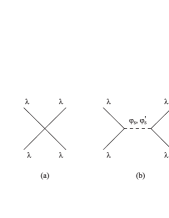
Figure 4: Tree–level Feynman diagrams contributing to the four-gaugino scattering amplitudes: (a) contact interactions; (b) $(\varphi_{S},\varphi_{S}^{\prime})$ exchange (the dots stand for the $t$- and $u$- channel diagrams.

The Lagrangian term (A.22) generates the contact interaction (fig. 4a)

$$-{1\over 4}{|M|^{2}\over|F|^{2}}\lambda\lambda\overline{\lambda}\overline{\lambda}\,,$$ (2.45)

which is again controlled by a model-independent coupling. At low energy ($s\ll m_{S}^{2},m_{S^{\prime}}^{2}$), this interaction should be considered together with diagrams with virtual ${\varphi_{S}},{\varphi_{S}^{\prime}}$ exchange (fig. 4b), controlled by the cubic couplings (2.20). However, no special cancellation emerges in this case, where no goldstinos are involved. At high energy, the contact interaction dominates and produces an amplitude growing as $E^{2}|M|^{2}/|F|^{2}$ and a cross section growing as $\sigma\sim s|M|^{4}/|F|^{4}$. Once again, unitarity is broken for $s\gg|F|^{2}/|M|^{2}$ and the consistency condition that the critical energy be larger than $|M|$ leads to a bound $|M|^{2}<{\cal O}(10)|F|$, of the same form as the previous bound (2.28).

2.3.5 $\tilde{S}\tilde{S}\tilde{A}\tilde{A}$

Finally, we discuss processes involving two goldstinos and two ${\tilde{A}}$ fermions, described by the Feynman diagrams of fig. 5.

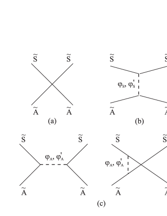
Figure 5: Tree–level Feynman diagrams contributing to the goldstino-$\tilde{A}$ scattering amplitudes: (a) contact interactions; (b) $(\varphi_{S},\varphi_{S}^{\prime})$ exchange; (c) $(\varphi_{A},\varphi_{A}^{\prime})$ exchange.

The Lagrangian term (A.23) generates the following contact interactions (fig. 5a):

$${1\over 4}\left\langle{{\tilde{H}}_{SS}-{\tilde{H}}_{S}\Gamma^{S}_{SS}\over{\tilde{K}}{\hat{K}}_{\overline{S}S}}\right\rangle\tilde{S}\tilde{S}\overline{\tilde{A}}\overline{\tilde{A}}+{\rm h.c.}\,,$$ (2.46)

$$-{m_{A}^{2}+m_{A^{\prime}}^{2}-2m_{\tilde{A}}^{2}\over 2|F|^{2}}\tilde{S}\tilde{A}\overline{\tilde{S}}\overline{\tilde{A}}\,.$$ (2.47)

These interactions should be considered together with diagrams with ${\varphi_{S}},{\varphi^{\prime}_{S}}$ exchange (fig. 5b), controlled by the cubic couplings (2.21), (2.29) and (2.30), and diagrams with ${\varphi_{A}},{\varphi^{\prime}_{A}}$ exchange (fig. 5c), controlled by the cubic coupling (2.31). We start by discussing the low-energy properties. If we integrate out the scalars ${\varphi_{S}},{\varphi^{\prime}_{S}}$, we obtain the effective interaction

$$-{1\over 4}\left\langle{{\tilde{H}}_{SS}-{\tilde{H}}_{S}\Gamma^{S}_{SS}\over{\tilde{K}}{\hat{K}}_{\overline{S}S}}\right\rangle\tilde{S}\tilde{S}\overline{\tilde{A}}\overline{\tilde{A}}+{\rm h.c.}\,,$$ (2.48)

which cancels the above contact term (2.46). At the same time, a new term

$${1\over 8}{m^{2}_{A}-m^{2}_{A^{\prime}}\over F^{2}}\tilde{S}\tilde{S}{\tilde{A}}{\tilde{A}}+{\rm h.c.}$$ (2.49)

is generated. To continue the discussion of the low-energy limit and include the ${\varphi_{A}},{\varphi^{\prime}_{A}}$ exchange contributions, we consider two different cases. The simplest one corresponds to assuming $m_{\tilde{A}}\simeq 0$ and $m^{2}_{A^{\prime}}\simeq m^{2}_{A}\gg s$. Then the term (2.49) is absent and the remaining term (2.47) is exactly cancelled by the leading contribution from integrating out ${\varphi_{A}},{\varphi^{\prime}_{A}}$. The situation is similar to the four-goldstino case: the leading low-energy behaviour for the amplitudes has the form $E^{4}/|F|^{2}$ instead of $E^{2}m_{A}^{2}/|F|^{2}$ and the corresponding cross sections scale as $\sigma\sim s^{3}/|F|^{2}$. Now let us consider a more general situation, with $m_{\tilde{A}}\neq 0$. We focus on the scattering process ${\tilde{S}}{\tilde{A}}\rightarrow{\tilde{S}}{\tilde{A}}$, since cancellations are more effective than in the annihilation processes, thanks to the low-energy theorems of supersymmetry [12]. In particular, we consider a Thomson-like low-energy limit where the incident goldstino has energy $E\ll m_{\tilde{A}}$ in the centre-of-mass frame, so that $s\simeq u\simeq m_{\tilde{A}}^{2}$ and $t\simeq 0$. Note that, for the different helicity choices, the scattering amplitudes receive ${\varphi_{A}},{\varphi^{\prime}_{A}}$ exchange contributions only in the $s$ and $u$ channels. Therefore, in that limit, the propagator denominators contain the same scalar-fermion mass splittings appearing in the attached cubic vertices (2.31). The explicit evaluation shows that an amplitude receiving a contribution from the contact term (2.47) is cancelled by either $s$- or $u$-channel ${\varphi_{A}},{\varphi^{\prime}_{A}}$ exchange, whereas an amplitude receiving a contribution from the term (2.49), which corresponds here to $t$-channel ${\varphi_{S}},{\varphi^{\prime}_{S}}$ exchange, is cancelled by the combined $s$-channel and $u$-channel ${\varphi_{A}},{\varphi^{\prime}_{A}}$ exchange. As a result, the leading amplitudes scale with $E^{2}m_{\tilde{A}}^{2}/|F|^{2}$ instead of growing linearly with $E$, and the corresponding cross sections scale as $\sigma\sim E^{4}m^{2}_{\tilde{A}}/|F|^{4}$. Finally, we briefly comment on the high-energy régime, considering for simplicity the case in which $m_{\tilde{A}}\simeq 0$ and the scalars have a common mass $m^{2}<s$. Then the situation is similar to the case of four-goldstino scattering. The contact interaction (2.47) generates scattering amplitudes that grow as $sm^{2}/|F|^{2}$ and cross sections that grow as $\sigma\sim sm^{4}/|F|^{4}$, so for $s\gg|F|^{2}/m^{2}$ unitarity breaks down. The condition that the critical energy be larger than $m$ leads to a bound of the form $m^{2}<{\cal O}(10)|F|$, similar to those already discussed in the present and previous subsections.

2.4 Goldstino (light gravitino) phenomenology

The results of the present section can easily be extended from the class of models we have used for illustrative purposes to realistic models, with gauge group $SU(3)\times SU(2)\times U(1)$ (or larger), and matter content including, besides the goldstino supermultiplet, also quark, lepton and other chiral supermultiplets. In particular, we can consider generalizations where the $S$ field remains a gauge singlet, while the $A$ field is replaced by a set of charged multiplets (for example the MSSM fields), coupled to the gauge sector via ‘usual’ gauge interactions. As explained in the introduction, our effective theory description, based on spontaneously broken $N=1$ global supersymmetry, will be adequate as long as the goldstino couplings to the supercurrent are larger than the gravitational ones, that is ${\Lambda}_{S}^{4}<\Delta m^{2}M_{\rm P}^{2}$, and we consider experiments performed at energies $E$ larger than the gravitino mass and smaller than the unitarity bounds, that is $({\Lambda}_{S}^{4}/M_{\rm P}^{2})\stackrel{{\scriptstyle<}}{{{}_{\sim}}}E^{2}\stackrel{{\scriptstyle<}}{{{}_{\sim}}}({\Lambda}_{S}^{4}/\Delta m^{2})$.

To put things in perspective, we recall that, when discussing the phenomenology of supersymmetric extensions of the Standard Model, under the assumption of supersymmetry-breaking mass splittings of the order of the electroweak scale, it is useful to distinguish three main possibilities

a) Heavy gravitino.    If the scale of supersymmetry breaking is the geometrical mean of the electroweak and Planck scales, the gravitino mass is of the order of the electroweak scale, and the gravitino couplings to all the other fields have gravitational strength. This is the case of the so-called hidden sector supergravity models. The effective theory near the electroweak scale [19] is the MSSM [20], a renormalizable theory with explicit but soft [21] breaking of supersymmetry. The additional non-renormalizable operators of the underlying supergravity theory, involving the gravitino and associated with the spontaneous breaking of local supersymmetry, are suppressed by inverse powers of the Planck mass. Such a property also allows a consistent extrapolation of the MSSM up to a possible scale of supersymmetric grand unification, since tree-level unitarity is violated only close to the Planck scale. As for the phenomenology at colliders, this is the most studied case (see, e.g., ref. [22]): the lightest supersymmetric particle is, in most of the cases, an admixture of neutral gauginos and higgsinos, or neutralino, and the footprint of supersymmetric particle production is the missing energy associated with the undetected neutralino.

b) Light gravitino.    If the scale of supersymmetry breaking is only a few orders of magnitude above the electroweak scale, say between 10 and 100 TeV, then the gravitino mass is in the eV–keV range, and the goldstino couplings to the MSSM fields have strength much greater than the gravitational one. This is the case of most models of dynamical supersymmetry breaking currently under study [7]. For most practical purposes, we can still take the MSSM as an effective theory near the electroweak scale, since the additional operators involving the goldstino and associated with the spontaneous breaking of global supersymmetry are considerably suppressed with respect to the renormalizable MSSM operators. However, in this case we cannot in general extrapolate the MSSM up to a possible scale of supersymmetric grand unification, since tree-level unitarity is violated at a much smaller scale. To make such an extrapolation possible, we have to include the (model-dependent) degrees of freedom that play a rôle in the restoration of unitarity: in the so-called messenger models [7], for example, this rôle is played by the messenger fields. As for the phenomenology at collider energies accessible at present, if the lightest supersymmetric particle besides the gravitino is a neutralino with non-negligible photino component, then the only modification with respect to the previous case is due to the effects of the operator (2.26), which allows for the decay of the lightest neutralino into a photon plus a goldstino (light gravitino). In this case, the footprints of supersymmetric particle production are both missing energy and photons, with a photon spectrum dictated by the mass of the lightest neutralino. There is also room for a sfermion to be the lightest supersymmetric particle besides the gravitino: in such a case operators of the form (2.31) control its decays into the corresponding fermion plus a goldstino (light gravitino), and we fall back to more conventional missing energy signals, with the only difference that the undetected particle is now the gravitino. Recent work on supersymmetric phenomenology at colliders in the presence of a light gravitino can be found in refs. [23].

c) Superlight gravitino.    If the scale of supersymmetry breaking is very close to the electroweak scale, then the gravitino is superlight, with a mass in the $10^{-5}$ eV range, and the goldstino couplings to the MSSM fields have a strength comparable to the renormalizable MSSM couplings. In this case, in order to discuss the phenomenology at the electroweak scale we must consider at least the full effective theory discussed in the present paper, taking also into account its limitations when we approach the unitarity bounds. It is also clear that the energy range of validity of our effective theory description is very limited, and we should replace it with a more fundamental theory not much above the electroweak scale. The interesting point of such a possibility is that it could give rise, at the present collider energies, to a phenomenology that is radically different from the previous two cases. Such phenomenology should also allow us to establish model-independent lower bounds on the scale of supersymmetry breaking, and therefore on the gravitino mass, without making reference to the actual masses of the supersymmetric particles in the MSSM. For example, we could consider scattering processes where the initial state is made of ordinary particles (quarks, leptons, gauge bosons), whereas the final state contains both ordinary particles and goldstinos (superlight gravitinos), and use the phenomenological bounds on the corresponding rates.

In the following, we will discuss some aspects of the superlight gravitino phenomenology that are strictly related to the results of the present section.

2.4.1 Collider signatures of a superlight gravitino

At $e^{+}e^{-}$ high-energy colliders, such as LEP or the proposed Next Linear Collider, we could consider processes such as $e^{+}e^{-}\to\tilde{S}\tilde{S}\gamma$ or $e^{+}e^{-}\to e^{+}e^{-}\tilde{S}\tilde{S}$, and similar processes could be considered at hadron colliders, such as the Tevatron or the LHC. Indeed, this was already done in the past [25], but always under special assumptions on the supersymmetric particle spectrum, such as light gauginos or light spin-0 superpartners of the goldstino: the resulting limits on the gravitino mass, of the order of $10^{-6}{\rm\;eV}$, are therefore model-dependent. To perform a general and reliable analysis of the above processes, including the latest experimental data from LEP and the Tevatron collider, would require a considerable amount of work: we should generalize the formalism, compute the relevant cross sections in the general case, scan the different ranges of supersymmetric particle masses, and compare the results with experimental data and background calculations. We postpone all this to future work. We can already anticipate, however, that the weakening of the old bounds due to the greater generality will be approximately compensated by the higher energies accessible at the present machines.

2.4.2 The processes $\gamma\gamma\longleftrightarrow\tilde{S}\tilde{S}$

The formalism developed in this paper is already sufficient to comment on some cosmological and astrophysical bounds on the gravitino mass, which were previously studied in connection with the annihilation processes $\gamma\gamma\to\tilde{S}\tilde{S}$ and $\tilde{S}\tilde{S}\to\gamma\gamma$. To set the framework, we have computed the general expression for the total cross-section of the two processes:

$$\sigma(\gamma\gamma\to\tilde{S}\tilde{S})=\sigma(\tilde{S}\tilde{S}\to\gamma\gamma)={|M|^{6}\over 32\pi|F|^{4}}\left(C_{0}+C_{1}\log{|M|^{2}\over s+|M|^{2}}\right)\,,$$ (2.50)

where

$$C_{0} = {m_{S}^{8}\over 4(s-m_{S}^{2})^{2}|M|^{4}}+{m_{S^{\prime}}^{8}\over 4(s-m_{S^{\prime}}^{2})^{2}|M|^{4}}+{m_{S}^{4}(m_{S}^{2}+2|M|^{2})\over 2(s-m_{S}^{2})|M|^{4}}+{m_{S^{\prime}}^{4}(m_{S^{\prime}}^{2}+2|M|^{2})\over 2(s-m_{S^{\prime}}^{2})|M|^{4}}$$ (2.51)

$$+ {m_{S}^{4}+m_{S^{\prime}}^{4}+4(m_{S}^{2}+m_{S^{\prime}}^{2})|M|^{2}+4|M|^{4}\over 4|M|^{4}}-{4|M|^{2}\over s}+{|M|^{2}\over s+|M|^{2}}+{s\over 6|M|^{2}}\,,$$

and

$$C_{1}={m_{S}^{2}\over s-m_{S}^{2}}+{m_{S^{\prime}}^{2}\over s-m_{S^{\prime}}^{2}}+{|M|^{2}\over s+2|M|^{2}}-{4|M|^{4}\over s^{2}}\,.$$ (2.52)

As in the previous literature, we have assumed that the photino is a mass eigenstate: to be completely general, we should include the possibility of gaugino–higgsino mixing. In the special limits $s\gg m_{S}^{2},m_{S^{\prime}}^{2},|M|^{2}$ and $m_{S}^{2},m_{S^{\prime}}^{2}\ll s,|M|^{2}$ our results are in agreement with the supergravity results of refs. [16] and [17], respectively. We now focus on the low-energy limit, $s\ll|M|^{2},m_{S}^{2},m_{S^{\prime}}^{2}$, where the expressions for the scattering amplitudes in the individual helicity channels and for the total unpolarized cross-section simplify considerably. Indeed, the leading contributions to the amplitudes and the cross-section become independent of the the scalar and gaugino masses, as anticipated in section 2.3.2 and summarized by the effective operator of eq. (2.40). Removing an irrelevant overall phase, and denoting by ${\cal A}(\lambda_{1},\lambda_{2},\sigma_{1},\sigma_{2})$ the scattering amplitude for photon helicities $\lambda_{1,2}$ and goldstino helicities $\sigma_{1,2\;}$, we find

$${\cal A}(+1,-1;+1/2,-1/2)={\cal A}(-1,+1;-1/2,+1/2)=8\sin\theta\cos^{2}(\theta/2)E^{4}/|F|^{2}\,,$$ (2.53)

$${\cal A}(+1,-1;-1/2,+1/2)={\cal A}(-1,+1;+1/2,-1/2)=-8\sin\theta\sin^{2}(\theta/2)E^{4}/|F|^{2}\,,$$ (2.54)

where $E$ and $\theta$ are the energy of each particle and the scattering angle in the centre-of-mass frame, respectively. The remaining helicity channels have amplitudes proportional to higher powers of $E$. The total cross-section then becomes:

$$\sigma(\gamma\gamma\to\tilde{S}\tilde{S})=\sigma(\tilde{S}\tilde{S}\to\gamma\gamma)={s^{3}\over 640\pi|F|^{4}}+\ldots\,.$$ (2.55)

Here, as already stated, our results differ from those of ref. [9]. We would like to add that the low-energy limit allows also to relax the assumption that the photino be a mass eigenstate. In particular, we have checked that the results (2.40) and (2.53)–(2.55) remain valid in the realistic case where the gauge group is the Standard Model one and neutralino mixing is taken into account, at least if the goldstino belongs to a gauge singlet chiral superfield, the gauge kinetic function factorizes with respect to the gauge group factors, and the $D$-terms have vanishing vacuum expectation values.

Very light and stable gravitinos can affect the standard nucleosynthesis scenario [8, 9, 10]: if the decoupling temperature of goldstinos from the early universe thermal bath is sufficiently small, gravitinos can contribute to the number $N_{\nu}$ of effective neutrino species, which is bounded from above by cosmological analyses [26]. The corresponding bound on the gravitino mass strongly depends on the assumed bound on $N_{\nu}$, $N_{\nu}^{max}$, and may be more stringent than particle physics bounds only if $N_{\nu}^{max}$ is significantly smaller than 4. In previous analyses, the dominant reaction affecting the gravitino thermal equilibrium was considered to be the annihilation process $\gamma\gamma\leftrightarrow\tilde{S}\tilde{S}$, on the basis of a cross section assumed to grow as $\sigma\sim s^{2}|M|^{2}/|F|^{4}$. However, if there are no superlight non-standard particles (with mass $\stackrel{{\scriptstyle<}}{{{}_{\sim}}}100{\;\rm MeV}$) besides the gravitino, the relevant cross-section is that of eq. (2.55): this means that even the bounds of [9, 10], which in turn were considerably weaker than previous ones [8], should be revised. For example, using $N_{\nu}<3.6$, ref. [9] found $m_{3/2}\stackrel{{\scriptstyle>}}{{{}_{\sim}}}10^{-6}{\rm\;eV}$ (for $|M|\sim 100{\rm\;GeV}$), whereas on the basis of (2.55) we estimate a bound about a factor $10^{1-2}$ weaker; to be more precise, we would need to consider all the reactions that now become competitive with $\gamma\gamma\leftrightarrow\tilde{S}\tilde{S}$, but the bounds now become so weak, compared with those coming from high-energy accelerators, that the effort is probably unjustified.

For very light gravitinos and heavy $(\lambda,S,S^{\prime})$, the annihilation process $\gamma\gamma\to\tilde{S}\tilde{S}$ can also be relevant for stellar cooling [8, 9, 10] (other processes that may contribute to stellar cooling were considered in [27]). Again, using a cross-section going as $\sigma\sim s^{2}|M|^{2}/|F|^{4}$ and the observed neutrino luminosity from Supernova 1987a, ref. [10] claimed to exclude the range $2.6\times 10^{-8}{\rm\;eV}<m_{3/2}<2.2\times 10^{-6}{\rm\;eV}$. Using eq. (2.55), we estimate that the bounds of [10] should be reduced by a factor of about $10^{1-2}$, losing in part their interest when compared with possible accelerator bounds. Establishing a precise bound, however, would require the examination of all other processes that may become competitive with the above annihilation as a mechanism for stellar cooling.

2.5 Explicit models

We will now present some explicit and simple models of the type discussed above, not only to see the previous general considerations at work on some specific example, but also to prove the existence of models whose vacuum has the general properties discussed so far. For simplicity, in the chiral superfield sector we put initially $A$ to zero, and consider only $S$.

2.5.1 Canonical kinetic terms

To begin with, we consider the simple case of canonical kinetic terms, $K=|S|^{2}$ and $f=1/g^{2}$. The unique superpotential that leads to a supersymmetry breaking vacuum is then $w=\Lambda_{S}^{2}\,S$, where ${\Lambda}_{S}$ should be interpreted as some dynamical scale, induced in the effective theory by non-perturbative phenomena of the microscopic theory. In such a model, the scalar potential is just a constant: $V=||F||^{2}\equiv{\Lambda}_{S}^{4}$. Thus $V$ is minimized for arbitrary values of $S$, and all the configurations along this complex flat direction break spontaneously global supersymmetry, with order parameter ${\Lambda}_{S}$. The uniqueness of the supersymmetry-breaking superpotential linear in $S$, in the case of canonical kinetic terms considered here, is easily proved. For a generic superpotential $w(S)$, $V=|w^{\prime}(S)|^{2}$, and, from elementary theorems in complex analysis, $V$ can have a positive relative minimum if and only if $w^{\prime}(S)\equiv c\neq 0$, so that $w(S)=aS+b$, with $b$ irrelevant for global supersymmetry.

2.5.2 Embedding in supergravity

The previous model can be viewed as an ultra-minimal example exhibiting the spontaneous breaking of global supersymmetry. The physics remains trivial in spite of supersymmetry breaking, because the canonical choices for $K$ and $f$ do not lead to any masses or interactions. However, we will see below that a non-trivial physical content can be easily obtained by departing from canonicity. Before doing that, we will briefly comment on a locally supersymmetric generalization of the above model, where one of the ingredients is also a certain departure from canonicity. Indeed, the above model can be easily obtained, by taking the appropriate low-energy limit, from a corresponding non-trivial supergravity model where supersymmetry is spontaneously broken and in addition the vacuum energy vanishes. Normalizing the fields conveniently, the underlying supergravity model can be defined via the $SU(1,1)/U(1)$ Kähler potential

$$K=-3\,M_{\rm P}^{2}\log\left(1-{1\over 3}{|S|^{2}\over M_{\rm P}^{2}}\right)$$ (2.56)

and the superpotential

$$w={M_{\rm P}{\Lambda}_{S}^{2}\over\sqrt{3}}\left(1+{S\over\sqrt{3}M_{\rm P}}\right)^{3}\,.$$ (2.57)

The scalar potential, which now includes the gravitational contribution, is identically vanishing: $V=||F||^{2}-||H||^{2}\equiv 0$. Comparing with the global case, we see that the welcome effect of the gravitational interactions is the removal of the constant term $\Lambda_{S}^{4}$ and the consequent vanishing of the ‘true’ vacuum energy. Notice that, if one is interested in the $M_{\rm P}\to\infty$ limit only, the globally supersymmetric model can be directly derived from the supergravity one by keeping only the leading terms in the $1/M_{\rm P}$ expansion of $K$ and $w$:

$$K=|S|^{2}+{\cal O}\left({S^{4}\over M_{\rm P}^{2}}\right)\,,$$ (2.58)

$$w={M_{\rm P}{\Lambda}_{S}^{2}\over\sqrt{3}}+{\Lambda}_{S}^{2}\,S+{\cal O}\left({{\Lambda}_{S}^{2}S^{2}\over M_{\rm P}}\right)\,,$$ (2.59)

and by discarding the constant term in the superpotential. We finally remark that, when the limit $M_{\rm P}\to\infty$ with ${\Lambda}_{S}$ fixed is taken, the gravitino mass $m_{3/2}^{2}\equiv\langle e^{K/M_{\rm P}^{2}}|w|^{2}/M_{\rm P}^{4}\rangle$ vanishes as $m_{3/2}\sim{\Lambda}_{S}^{2}/M_{\rm P}$, whereas the product $m_{3/2}M_{\rm P}\sim{\Lambda}_{S}^{2}$ remains constant and identifies the (fixed) supersymmetry breaking scale.

2.5.3 Non-canonical kinetic terms

We now go back to the globally supersymmetric model considered above and discuss how more general versions can be obtained using non-canonical gauge kinetic function and Kähler potential. Of course, even the simple model considered above can be reformulated using non-canonical functions. For example, the analytic field redefinition $S=(S^{\prime})^{2}/{\Lambda}_{S}$ would transform the superpotential into $w={\Lambda}_{S}(S^{\prime})^{2}$ and the Kähler potential into $K=|S^{\prime}|^{4}/{\Lambda}_{S}^{2}$, therefore inducing a fake singularity of the Kähler metric at the origin. However, as guaranteed by general theorems, the physical content of the model would remain the same. In the search for less trivial versions, one can consider for instance Kähler potentials that admit a power expansion around the canonical form.

A minimal non-trivial example can be built by keeping the form $w=\Lambda_{S}^{2}\,S$ for the superpotential and modifying the Kähler potential and gauge kinetic function as follows:

$$K=|S|^{2}-{|S-v|^{4}\over 4{\Lambda}^{2}}\,,$$ (2.60)

$$f={1\over g^{2}}\left(1+{S-v\over{\Lambda}_{f}}\right)\,.$$ (2.61)

Here $v$, ${\Lambda}$ and ${\Lambda}_{f}$ are real and positive mass parameters, which control the deviations from the canonical forms of $K$ and $f$, recovered in the limit ${\Lambda},{\Lambda}_{f}\to\infty$. The choice (2.60) leads to a Kähler metric $K_{\overline{S}S}=1-|S-v|^{2}/{\Lambda}^{2}$, so that the allowed field configurations, corresponding to a positive-definite Kähler metric, are those satisfying the inequality $|S-v|<{\Lambda}$. Thus the scale ${\Lambda}$, which controls the deviations from a canonical Kähler potential, acts also as an effective cutoff in field space. The scalar potential is now

$${||F||^{2}=\displaystyle{{{\Lambda}_{S}^{4}\over 1-\displaystyle{{|S-v|^{2}\over{\Lambda}^{2}}}}}}\,.$$ (2.62)

It is manifestly positive-definite in the domain of validity of the model and has an absolute minimum for $\langle S\rangle=v$, where $\langle||F||^{2}\rangle={\Lambda}_{S}^{4}$. Supersymmetry is spontaneously broken with order parameter ${\Lambda}_{S}$ as before and the gauge and Kähler metrics are canonical only at the minimum. Since the $S$ direction is no longer flat, the scalars $\varphi_{S}$ and $\varphi_{S}^{\prime}$ now have non-vanishing masses,

$$m_{S}^{2}=m_{S^{\prime}}^{2}={{\Lambda}_{S}^{4}\over{\Lambda}^{2}}\,,$$ (2.63)

controlled by the supersymmetry-breaking scale and the curvature of the Kähler manifold at the minimum of the potential. Similarly, a non-vanishing gaugino mass is generated,

$$M={{\Lambda}_{S}^{2}\over 2{\Lambda}_{f}}\,,$$ (2.64)

controlled by the supersymmetry-breaking scale and ${\Lambda}_{f}$.

Besides generating non-vanishing masses, the non-canonical $K$ and $f$ also generate non-trivial interactions, which are special cases of the ones discussed in the previous subsections. In particular, the general bounds (2.19), (2.23) and (2.28) relating masses and $|F|$ can be converted into the following bounds relating ${\Lambda}_{S}$, ${\Lambda}$ and ${\Lambda}_{f}$:

$${\Lambda}_{S}^{2}<2\sqrt{32\pi}{\Lambda}{\Lambda}_{f}\,,\;\;\;\;\;{\Lambda}_{S}^{2}<\sqrt{32\pi}{\Lambda}^{2}\,,\;\;\;\;\;{\Lambda}_{S}^{2}<4\sqrt{16\pi}{\Lambda}_{f}^{2}\,.$$ (2.65)

We recall that such relations come from the requirement that certain effective cubic couplings be not too large. Similarly, one can specialize to the present case the unitarity bounds derived from the study of four-particle processes. For instance, the critical energy (2.37), which signals the unitarity breakdown in the four-goldstino amplitudes, now becomes directly related to the scale ${\Lambda}$:

$$\sqrt{s}_{c}=\sqrt{24\pi}{\Lambda}\,.$$ (2.66)

As a consequence, the requirement $s_{c}>m_{S}^{2}+m_{S^{\prime}}^{2}$, leading to (2.38), now gives

$${\Lambda}_{S}^{2}<\sqrt{12\pi}{\Lambda}^{2}\,,$$ (2.67)

which is consistent with the second inequality in (2.65).

As a final remark, we note that the $A$ field could be easily added to the above toy model. In particular, a mass splitting in the $A$ sector can be generated by choosing a non-canonical metric ${\tilde{K}}(S,{\overline{S}})$, in the notation of (2.2). For example, the simple choice

$${\tilde{K}}=1-{|S-v|^{2}\over{\tilde{\Lambda}}^{2}}\,$$ (2.68)

leads to a metric that is canonical only at the minimum and that induces, according to eq. (2.12), scalar soft masses

$${\tilde{m}}^{2}_{A}={{\Lambda}_{S}^{4}\over{\tilde{\Lambda}}^{2}}\,.$$ (2.69)

In particular, the scales ${\Lambda}_{S}$, ${\Lambda}$, ${\Lambda}_{f}$ and $\tilde{{\Lambda}}$ may coincide with a single dynamically generated scale of an underlying microscopic theory and still remain compatible with the bounds (2.65) and (2.67).

3 The case of a non-singlet goldstino

In this section, we will examine some special features of models where the spontaneous breaking of $N=1$ global supersymmetry is strictly related with the spontaneous breaking of the gauge symmetry, and the goldstino is charged under the broken gauge group. Our aim is to show that, while most of the general results of the previous section can be easily adapted to the new framework, the constraints coming from gauge invariance lead to an increased predictive power and to new effects. In particular, we will show that the singularity structure of the defining functions of the model, needed to spontaneously break both supersymmetry and gauge symmetry, leads to a special class of interactions, controlled by the scales of gauge and supersymmetry breaking, and that the latter are subject to peculiar constraints from tree-level unitarity.

For our purpose, it will be sufficient to consider the class of $N=1$ globally supersymmetric models with gauge group $G=U(1)_{Y}$ and two chiral superfields $(H_{1},H_{2})$ of opposite non-vanishing charges, conventionally normalized to $Y(H_{1})=-1/2$ and $Y(H_{2})=+1/2$. We assume that no Fayet–Iliopoulos term is present: thanks to the non-anomalous field content of the theory, this situation is stable against perturbative quantum corrections. We start with two very simple observations, which have important implications. First, if supersymmetry is spontaneously broken, then the gauge symmetry must be broken at the same time, since these models do not contain neutral superfields. Second, if the superpotential $w$, the gauge kinetic function $f$ and the Kähler metric $K_{\overline{\j}i}$ have no singularities (including zeros) at the origin, so that they can be Taylor-expanded around $H_{1}=H_{2}=0$, then supersymmetry is unbroken. In fact, gauge invariance forces the first terms in the Taylor expansions of $w$ and $K$ to be at least quadratic in the fields; thus both $F_{i}\equiv w_{i}$ and $D_{Y}\equiv Y_{(i)}K_{i}\varphi^{i}$ vanish at the origin, and so does the potential $V=||F||^{2}+||D||^{2}$. This important result is indeed valid for any $N=1$ globally supersymmetric model that does not contain gauge-singlet chiral superfields nor a Fayet–Iliopoulos term, irrespective of the gauge group and of the representation content: a necessary condition for supersymmetry breaking is the singular behaviour at the origin of one of the defining functions of the model. In the following, for definiteness, we will consider models where the singularity at the origin comes from the superpotential, whereas the Kähler potential and the gauge kinetic function admit a power expansion around their canonical form.

We would like to study the peculiar features of our class of models without excessive complications, limiting ourselves to the case of pure $F$-term supersymmetry breaking. Notice that the basic functions $w$ and $f$ are necessarily symmetric under $H_{1}\leftrightarrow H_{2}$, since they must be functions of the only available analytic invariant $H_{1}H_{2}$. For simplicity, we will assume that $K$ is symmetric as well. For the moment, we do not discuss the minimization of the scalar potential: we just assume the existence of a minimum that breaks both gauge symmetry and supersymmetry, with $\langle||F||^{2}\rangle\neq 0$, $\langle||D||^{2}\rangle=0$. Notice that in general the minimum of the potential can be parametrized by the three real gauge-invariant variables $v_{1}$, $v_{2}$ and $\theta$, defined by $\langle|H_{1}|^{2}\rangle\equiv v_{1}^{2}$, $\langle|H_{2}|^{2}\rangle\equiv v_{2}^{2}$ and $\langle H_{1}H_{2}\rangle\equiv v_{1}v_{2}e^{2\i\theta}$. However, our assumptions of symmetric $K$ and no $D$-term breaking imply $v_{1}=v_{2}\equiv v/\sqrt{2}$, and we can always gauge-rotate the fields so that $\langle H_{1}\rangle=\langle H_{2}\rangle=ve^{\i\theta}/\sqrt{2}$. Moreover, in order to make contact with the formalism of the previous section, it is convenient to introduce the symmetric and antisymmetric combinations of fields:

$$S\equiv{H_{1}+H_{2}\over\sqrt{2}}\,,\;\;\;\;\;A\equiv{H_{1}-H_{2}\over\sqrt{2}}\,.$$ (3.1)

The fields defined in (3.1) are special cases of the $S$ and $A$ fields of section 2. In particular, they will satisfy the basic conditions (2.4), and $S$ will have a non-vanishing vev, $\langle S\rangle=ve^{\i\theta}$.

To discuss the mass spectrum around the chosen vacuum, it is sufficient to expand the defining functions of the model up to quadratic fluctuations in the fields with vanishing vevs, as in eqs. (2.1)–(2.3). However, now the functions of $S$ appearing as coefficients in the $A$-field expansion are not independent, since $S$ and $A$ originate from the same charged multiplets and are linked by gauge invariance. In particular, taking into account that $H_{1}$ and $H_{2}$ enter the defining functions of the model only via the gauge-invariant bilinears $|H_{1}|^{2}+|H_{2}|^{2}=|S|^{2}+|A|^{2}$ and $H_{1}H_{2}=(S^{2}-A^{2})/2$, the following field identities can be derived:

$${\hat{w}}_{S}(S)\equiv-S\,{\tilde{w}}(S)\,,$$ (3.2)

$${\hat{K}}_{S}(S,{\overline{S}})\equiv\overline{S}\,{\tilde{K}}(S,\overline{S})-S\,{\tilde{H}}(S,\overline{S})\,.$$ (3.3)

We can then discuss the structure of the mass spectrum by specializing the general formulae of section 2.1, taking into account the useful identities (3.2) and (3.3), and by including the effects of the standard gauge interactions. The mass of the gauge boson is given by:

$$m_{V}^{2}={g^{2}v^{2}\over 2}\,\langle{\tilde{K}}\rangle\,.$$ (3.4)

In the fermionic sector, we can identify on general grounds the massless goldstino with the symmetric higgsino combination, $\tilde{S}$. More specifically, the mass matrix has the form:

$$i\lambda,\tilde{A},\tilde{S}:\;\;\;\;\;{\cal M}_{1/2}=\left(\begin{array}[]{ccc}M&m_{V}&0\\ m_{V}&\hat{\mu}&0\\ 0&0&0\end{array}\right)\,,$$ (3.5)

where, using (3.2), (3.3) and (2.5) in the general formula (2.10),

$$\hat{\mu}=-\left\langle{\overline{S}\over S}\overline{F}^{\overline{S}}\left[\log\left(\overline{S}\,{\tilde{K}}\right)\right]_{\overline{S}}\right\rangle\,.$$ (3.6)

The spin-0 $S$ sector contains two physical scalars. In particular, if $\langle V_{SS}\rangle=\langle V_{{\overline{S}}{\overline{S}}}\rangle$, the mass eigenstates are just the real and imaginary parts of the shifted $S$ field, $\varphi_{S}$ and $\varphi_{S}^{\prime}$ (2.6). The corresponding mass eigenvalues have the general expressions (2.7), which can be further specialized if additional information on ${\hat{w}}(S)$ and ${\hat{K}}(S,\overline{S})$ is given. The spin-0 $A$ sector contains a physical scalar and the unphysical Goldstone boson absorbed by the massive gauge boson. The fact that the determinant of the $F$-term mass matrix vanishes is a consequence of the equality $m^{2}_{AA}=m^{2}_{A{\overline{A}}}\langle{\overline{S}}/S\rangle$, which in turn follows from the use of (3.2), (3.3) and (2.5) in the general formulae (2.11), (2.12) and (2.13). The physical scalar particle has mass

$$m_{A}^{2}=m_{V}^{2}+\hat{m}^{2}\,,$$ (3.7)

where

$$\hat{m}^{2}=2\left(|{\hat{\mu}}|^{2}+\left\langle{\overline{F}}^{\overline{S}}(-\log{\tilde{K}})_{\overline{S}S}F^{S}\right\rangle\right)\,.$$ (3.8)

In particular, if $\langle S\rangle=\langle\overline{S}\rangle$, the physical scalar and the Goldstone boson are just the real and imaginary parts of $A$, $\varphi_{A}$ and $\varphi^{\prime}_{A}$ (2.14).

We should now discuss the interactions of the chosen class of models. Besides those already studied in section 2, we should include ordinary gauge interactions and work out explicitly the interactions associated with the singular behaviour of the superpotential at the origin. Instead of attempting a general treatment, however, we choose to continue the discussion by switching directly to specific examples, stressing the properties that have more general validity. We make this choice both for simplicity and to provide ‘existence proofs’ of the non-trivial situation where supersymmetry and gauge symmetry are broken simultaneously. The explicit models that we will present are non-trivial extensions of the corresponding ones of section 2.5.

3.1 Explicit models: canonical kinetic terms

As in 2.5.1, we begin by considering the simple case of a canonical gauge kinetic function,

$$f={1\over g^{2}}\,,$$ (3.9)

and a canonical Kähler potential,

$$K=|H_{1}|^{2}+|H_{2}|^{2}=|S|^{2}+|A|^{2}\,.$$ (3.10)

Then the unique superpotential that leads to a supersymmetry-breaking vacuum is

$$w={\Lambda}_{S}^{2}\sqrt{2H_{1}H_{2}}={\Lambda}_{S}^{2}\sqrt{S^{2}-A^{2}}\,,$$ (3.11)

where the numerical factor $\sqrt{2}$ is just for convenience and an irrelevant additive constant has been omitted. In the above expression, ${\Lambda}_{S}$ should be interpreted as some dynamical scale, induced in the effective theory by non-perturbative phenomena of the microscopic theory. The presence of non-renormalizable interactions in the superpotential and the lack of analyticity at the origin (conical singularity of deficit angle $\pi$) should not come as a surprise, given the existing literature [28, 29] on non-perturbative phenomena in supersymmetric theories.

In the model defined by eqs. (3.9)–(3.11), the $F$-term and $D$-term contributions to the scalar potential are easily computed (see the appendix for the general formulae):

$$||F||^{2}={\Lambda}_{S}^{4}{|H_{1}|^{2}+|H_{2}|^{2}\over 2|H_{1}||H_{2}|}={\Lambda}_{S}^{4}+{\Lambda}_{S}^{4}{(|H_{2}|-|H_{1}|)^{2}\over 2|H_{1}||H_{2}|}\,,$$ (3.12)

$$||D||^{2}={g^{2}\over 8}\left(|H_{2}|^{2}-|H_{1}|^{2}\right)^{2}\,.$$ (3.13)

It is immediate to see that $V=||F||^{2}+||D||^{2}$ is positive definite, and is minimized for arbitrary values of $v_{1}=v_{2}\equiv v/\sqrt{2}$ and $\theta$. All the configurations along these two flat directions spontaneously break global supersymmetry, with order parameter $\langle||F||^{2}\rangle={\Lambda}_{S}^{4}$, and the $U(1)$ gauge symmetry. Conversely, it is easy to demonstrate the uniqueness of the superpotential (3.11), given the canonical terms (3.9) and (3.10). Since the only independent analytic invariant is $z\equiv H_{1}H_{2}$, the generic gauge-invariant superpotential can be written as $w(z)$, as already pointed out. Therefore the scalar potential reads

$$V=2\left|w^{\prime}(z)\sqrt{z}\right|^{2}+\left(|H_{2}|-|H_{1}|\right)^{2}\left[|w^{\prime}(z)|^{2}+{g^{2}\over 8}(|H_{2}|+|H_{1}|)^{2}\right]\,.$$ (3.14)

The two terms in (3.14) are separately positive semi-definite, and the second vanishes for $|H_{1}|=|H_{2}|$. This leaves the freedom to minimize the first term with respect to the complex variable $z$. From elementary theorems in complex analysis, $|w^{\prime}(z)\sqrt{z}|^{2}$ can have a positive relative minimum if and only if $w^{\prime}(z)\sqrt{z}\equiv c\neq 0$, so that $w(z)=a\sqrt{z}+b$, with $b$ irrelevant for global supersymmetry.

3.1.1 Masses and interactions

The computation of the masses and interactions around the generic vacuum is straightforward, and can be easily obtained by specializing the Lagrangian given in the appendix. In particular, the results for the spectrum agree with the general formulae given above. Since the mass eigenvalues turn out to be independent of $\theta$, for simplicity we will expand the Lagrangian around a minimum with $\theta=0$. Therefore the chosen vacuum has $\langle H_{1}\rangle=\langle H_{2}\rangle=v/\sqrt{2}$, i.e. $\langle S\rangle=v$ and $\langle A\rangle=0$.

The crucial feature of the model is the presence, besides the renormalizable gauge interactions, of a tower of non-renormalizable interactions, generated by the expansion of the superpotential (3.11) around the vacuum. The relevant terms of the Lagrangian are

$$||F||^{2} = \Lambda_{S}^{4}{|S|^{2}+|A|^{2}\over|S^{2}-A^{2}|}$$ (3.15)

$$= {\Lambda}_{S}^{4}+{{\Lambda}_{S}^{4}\over v^{2}}\varphi_{A}^{2}+{\cal O}\left({{\Lambda}_{S}^{4}\over v^{3}}\varphi^{3}\right)+{\cal O}\left({{\Lambda}_{S}^{4}\over v^{4}}\varphi^{4}\right)+{\cal O}\left({{\Lambda}_{S}^{4}\over v^{5}}\varphi^{5}\right)+\ldots\,,$$

where we have used the generic symbol $\varphi$ for any of the fields $(\varphi_{A},\varphi_{S},\varphi_{A}^{\prime},\varphi_{S}^{\prime})$, and

$${\cal L}_{YUK} = {{\Lambda}_{S}^{2}\over 2}{(A\tilde{S}-S\tilde{A})^{2}\over(S^{2}-A^{2})^{3/2}}+{\rm h.c.}$$ (3.16)

$$= \left[{1\over 2}{{\Lambda}_{S}^{2}\over v}\tilde{A}\tilde{A}-{{\Lambda}_{S}^{2}\over v^{2}}\left(\phi_{A}\tilde{S}\tilde{A}+{1\over 2}\phi_{S}\tilde{A}\tilde{A}\right)\right.$$

$$\left.+{{\Lambda}_{S}^{2}\over v^{3}}\left({1\over 2}\phi_{A}^{2}\tilde{S}\tilde{S}+2\phi_{S}\phi_{A}\tilde{S}\tilde{A}+{1\over 2}(\phi_{S}^{2}+3\phi_{A}^{2})\tilde{A}\tilde{A}\right)+\ldots\right]+{\rm h.c.}\,,$$

where $\phi_{S}\equiv S-v\equiv(\varphi_{S}+i\varphi^{\prime}_{S})/\sqrt{2}$ and $\phi_{A}\equiv A\equiv(\varphi_{A}+i\varphi^{\prime}_{A})/\sqrt{2}$. Among the renormalizable gauge interactions, we write down those involving fermions:

$${\cal L}^{\prime}={g\over 2}A_{\mu}{\overline{\tilde{A}}}{\overline{\sigma}}^{\mu}{\tilde{S}}-{ig\over\sqrt{2}}{\overline{\phi}}_{A}{\tilde{S}}\lambda-{ig\over\sqrt{2}}(v+{\overline{\phi}}_{S}){\tilde{A}}\lambda+{\rm h.c.}$$ (3.17)

We begin by summarizing the mass spectrum, part of which is already visible in the above expansions. Remembering that, in the notation of eq. (2.2), $\tilde{K}\equiv 1$, we find from (3.4) that the $U(1)$ gauge boson has a mass:

$$m_{V}={gv\over\sqrt{2}}\,.$$ (3.18)

In the spin-0 $S$ sector, we find that $m_{S}=m_{S^{\prime}}=0$. In the spin-0 $A$ sector, eq. (3.7) holds for the $\varphi_{A}$ mass, with

$$\hat{m}^{2}={2\Lambda_{S}^{4}\over v^{2}}\,,$$ (3.19)

whereas $\varphi^{\prime}_{A}$ is the unphysical Goldstone boson. In the fermionic sector, the mass matrix has the form (3.5), with $M=0$ and

$$\hat{\mu}=-{\Lambda_{S}^{2}\over v}\,.$$ (3.20)

The above mass spectrum exhibits a number of interesting features. Observe first that, since $\langle||D||^{2}\rangle=0$, the mass terms proportional to $gv$ are distributed in a supersymmetric way, in the sense that the contributions to ${\rm Str\;}{\cal M}^{2n}$ proportional to $(gv)^{2n}$ are identically vanishing for any positive integer $n$. Indeed, the supersymmetry-breaking mass splittings are all in the $(A,\tilde{A})$ sector, and are controlled by the ratio ${\Lambda}_{S}^{4}/v^{2}$; there are no mass splittings in the $(S,\tilde{S})$ sector. As already mentioned in section 2.1, this is a consequence of a general result of global supersymmetry [13]: for canonical kinetic terms and in the absence of anomalous $U(1)$ gauge factors, ${\rm Str\;}{\cal M}^{2}\equiv 0$ in each separate sector of the mass spectrum. In the $(A,\tilde{A})$ sector, where the fermion is massive, the two scalar degrees of freedom can have a mass splitting. In the $(S,\tilde{S})$ sector, which contains the massless goldstino, no mass splitting is allowed. Having in mind possible extensions to realistic models, the existence of massless scalars poses a potential problem. However, this can be solved by the introduction of non-canonical kinetic terms, as we have seen in section 2. Similar considerations apply to the diagonal gaugino mass term, which may be needed in realistic extensions of our toy model: its vanishing is due to the choice of a canonical gauge kinetic function $f$, but we know that a non-vanishing gaugino mass term can be generated by a non-canonical $f$. As a final comment on mass relations, notice that the non-renormalizable structure of the superpotential leads to violate a mass sum rule of the MSSM type: $m_{V}^{2}+m_{S^{\prime}}^{2}\neq m_{A}^{2}+m_{S}^{2}$.

By looking at eqs. (3.15) and (3.16), we can see that the ratio ${\Lambda}_{S}/v$ simultaneously controls all the operators of different dimensionality generated by the superpotential (3.11): the non-vanishing fermion and scalar masses are of order ${\Lambda}_{S}^{2}/v$; the $d=3$ cubic scalar operators have mass parameters of order ${\Lambda}_{S}^{4}/v^{3}$; the $d=4$ quartic scalar couplings and Yukawa couplings have dimensionless coefficients of order ${\Lambda}_{S}^{4}/v^{4}$ and ${\Lambda}_{S}^{2}/v^{2}$, respectively; the $d=5$ couplings of the type $\varphi^{5}$ or $\tilde{H}\tilde{H}\varphi^{2}$ have dimensionful coefficients of order ${\Lambda}_{S}^{4}/v^{5}$ and ${\Lambda}_{S}^{2}/v^{3}$, respectively, and so on. We then see that three qualitatively different situations are possible. If ${\Lambda}_{S}\ll v$, then the supersymmetry-breaking mass splittings are much smaller than the scale of gauge symmetry breaking, and the interactions induced by the superpotential are strongly suppressed by positive powers of ${\Lambda}_{S}/v$. An obvious physical application would be to identify the broken gauge group with some grand-unified group, as already attempted elsewhere [30, 11] in the supergravity context: the scale of supersymmetry breaking would then be ${\Lambda}_{S}\sim G_{F}^{-1/4}M_{\rm GUT}^{1/2}<G_{F}^{-1/4}M_{\rm P}^{1/2}$. If ${\Lambda}_{S}\sim v$, then the scales of gauge and supersymmetry breaking are the same, and all the operators in (3.15) and (3.16) have coefficients controlled by the appropriate power of this common scale: this will be the case, in a realistic framework, if the broken gauge group is identified with the Standard Model one. As we will see in a moment, tree-level unitarity strongly restricts the energy range in which the model is valid. Finally, the case ${\Lambda}_{S}\gg v$ corresponds to a strong coupling régime, where the scale of supersymmetry breaking is much larger than the scale of gauge symmetry breaking, and, for example, the dimensionless couplings of some $d=4$ operators become much larger than 1. To deal with this case consistently, we should remove the heavy degrees of freedom and consider a non-linear realization of supersymmetry in terms of the light degrees of freedom only.

The above discussion shows that, in spite of the canonical $K$ and $f$, the model under study can enter a strong coupling régime or violate unitarity, because $w$ generates couplings scaling with inverse powers of $v$. We can quantify such effects proceeding as in section 2. For simplicity, we will focus on those couplings and neglect the renormalizable gauge interactions, i.e. we will assume $g\ll{\Lambda}_{S}^{2}/v^{2}$. Notice that, since $m_{V}\ll|{\hat{\mu}}|$ in this limit, the fermion ${\tilde{A}}$ is a mass eigenstate with mass $|{\hat{\mu}}|$, whereas the scalar $\varphi_{A}$ has mass $m_{A}\simeq\sqrt{2}|{\hat{\mu}}|$. First, we can use two-body decays to constrain the parameter space where coupling constants are in the perturbative régime and a particle interpretation is allowed. For instance, we can consider the decay $\varphi_{A}\rightarrow\tilde{S}\tilde{A}$, controlled by one of the cubic Yukawa couplings of eq. (3.16). The calculation goes exactly as in section 2.2.6, and from the bound of eq. (2.33) we obtain:

$${\Lambda}_{S}<2\sqrt[4]{4\pi}v\simeq 4\,v\,.$$ (3.21)

In terms of $m_{A}$, this means $m_{A}\stackrel{{\scriptstyle<}}{{{}_{\sim}}}5{\Lambda}_{S}$, or $m_{A}\stackrel{{\scriptstyle<}}{{{}_{\sim}}}20v$. Second, we can use four-particle amplitudes to identify the energy scale characterizing unitarity violations, which is a cut-off scale for the effective theory. For instance, we can consider processes involving two $\varphi_{A}$ scalars and two goldstinos, i.e. ${\tilde{S}}\varphi_{A}\to{\tilde{S}}\varphi_{A}$, ${\tilde{S}}{\tilde{S}}\to\varphi_{A}\varphi_{A}$ and $\varphi_{A}\varphi_{A}\to{\tilde{S}}{\tilde{S}}$. In the high-energy limit, the leading contributions to the scattering amplitudes originate from the corresponding contact term of eq. (3.16):

$${{\Lambda}_{S}^{2}\over 4v^{3}}\varphi_{A}^{2}\tilde{S}\tilde{S}+{\rm h.c.}$$ (3.22)

This term generates amplitudes that grow as ${\sqrt{s}}{\Lambda}_{S}^{2}/v^{3}$, and unitarity breaks down beyond a critical energy ${\sqrt{s}_{c}}={\cal O}(10)v^{3}/{\Lambda}_{S}^{2}$. Notice that, for fixed $v$, $s_{c}$ decreases for increasing $\Lambda_{S}$. If we impose the consistency requirement $s_{c}>m_{A}^{2}$, we obtain bounds of the form ${\Lambda}_{S}\stackrel{{\scriptstyle<}}{{{}_{\sim}}}({\rm few})v$, as in (3.21).

3.1.2 Embedding in supergravity

The toy model of eqs. (3.9)–(3.11) should be viewed as a sort of minimal example exhibiting the simultaneous and spontaneous breaking of global supersymmetry and of gauge symmetry. In the context of local supersymmetry, i.e. supergravity, such an approach was previously studied in refs. [30, 31, 11]. We recall that, in the presence of gravitational interactions, the additional property of vanishing vacuum energy can be fulfilled at the same time. Indeed, it is instructive to see how our toy model can be obtained, by taking the appropriate low-energy limit, from one of the supergravity models with spontaneously broken supersymmetry and vanishing vacuum energy considered in ref. [11]. Normalizing conveniently the fields, the underlying supergravity model can be defined via the $(SU(1,1)/U(1))^{2}=SO(2,4)/SO(2)\times SO(4)$ Kähler potential

$$K=-{3\over 2}M_{\rm P}^{2}\log\left[\left(1-{2\over 3}{|H_{1}|^{2}\over M_{\rm P}^{2}}\right)\left(1-{2\over 3}{|H_{2}|^{2}\over M_{\rm P}^{2}}\right)\right]$$ (3.23)

and the superpotential

$$w={M_{\rm P}{\Lambda}_{S}^{2}\over\sqrt{3}}\left(1+\sqrt{2H_{1}H_{2}\over 3M_{\rm P}^{2}}\right)^{3}\,.$$ (3.24)

Since the $D$-term contribution to the scalar potential has the same form in local and global supersymmetry (see the appendix for the general formulae), we can concentrate on

$$||F||^{2}-||H||^{2} = \Lambda_{S}^{4}\frac{\left(1+{2|H_{1}H_{2}|\over 3M_{\rm P}^{2}}\right)\,\left|1+\sqrt{2H_{1}H_{2}\over 3M_{\rm P}^{2}}\right|^{4}}{\left(1-{2\over 3}{|H_{1}|^{2}\over M_{\rm P}^{2}}\right)^{3/2}\left(1-{2\over 3}{|H_{2}|^{2}\over M_{\rm P}^{2}}\right)^{3/2}}{(|H_{2}|-|H_{1}|)^{2}\over 2|H_{1}||H_{2}|}$$ (3.25)

$$= \Lambda_{S}^{4}{(|H_{2}|-|H_{1}|)^{2}\over 2|H_{1}||H_{2}|}\left[1+{\cal O}\left({H^{2}\over M_{\rm P}^{2}}\right)\right]\,.$$ (3.26)

The first line (3.25) shows that $||F||^{2}-||H||^{2}$ is positive semi-definite and vanishes identically along the supersymmetry- and gauge-symmetry-breaking minima $\langle|H_{1}|\rangle=\langle|H_{2}|\rangle$ (which make $||D||^{2}$ vanish as well). Of course, this property is inherited by the leading term (3.26) in the $1/M_{\rm P}$ expansion of $||F||^{2}-||H||^{2}$. Notice that (3.26) coincides with the field-dependent part of (3.12). The only (welcome) effect of the gravitational interactions, in the $M_{\rm P}\to\infty$ limit, is the removal of the constant term $\Lambda_{S}^{4}$ and the consequent vanishing of the ‘true’ vacuum energy. Notice also that, if one is interested in the $M_{\rm P}\to\infty$ limit only, the globally supersymmetric model can be directly derived from the supergravity one by keeping only the leading terms in the $1/M_{\rm P}$ expansion of $K$ and $w$:

$$K=|H_{1}|^{2}+|H_{2}|^{2}+{\cal O}\left({H^{4}\over M_{\rm P}^{2}}\right)\,,$$ (3.27)

$$w={M_{\rm P}{\Lambda}_{S}^{2}\over\sqrt{3}}+{\Lambda}_{S}^{2}\sqrt{2H_{1}H_{2}}+{\cal O}\left({{\Lambda}_{S}^{2}H^{2}\over M_{\rm P}}\right)\,,$$ (3.28)

and by discarding the constant term in the superpotential. We finally remark that, when the limit $M_{\rm P}\to\infty$ with ${\Lambda}_{S}$ fixed is taken, the gravitino mass $m_{3/2}^{2}\equiv\langle e^{K/M_{\rm P}^{2}}|w|^{2}/M_{\rm P}^{4}\rangle$ vanishes as $m_{3/2}\sim{\Lambda}_{S}^{2}/M_{\rm P}$, whereas the product $m_{3/2}M_{\rm P}\sim{\Lambda}_{S}^{2}$ remains constant and identifies the (fixed) supersymmetry-breaking scale.

3.2 Explicit models: non-canonical kinetic terms

The globally supersymmetric model described above is clearly non-trivial, in spite of the canonical Kähler potential and gauge kinetic function, and has allowed us to illustrate a number of important issues. We would like to comment here on more general versions of the model, characterized by non-canonical $K$ and $f$. Before moving to models with a different physical content, it may be useful to recall that models equivalent to the previous one can be easily obtained via analytic field redefinitions, which could in particular shift the singularity at the origin from the superpotential to the Kähler metric. For example, the redefinition $H_{1}=(H_{1}^{\prime})^{2}/{\Lambda}_{S}$, $H_{2}=(H_{2}^{\prime})^{2}/{\Lambda}_{S}$ would transform the Kähler potential into $K=(|H_{1}^{\prime}|^{4}+|H_{2}^{\prime}|^{4})/{\Lambda}_{S}^{2}$ and the superpotential into $w=\sqrt{2}{\Lambda}_{S}H_{1}^{\prime}H_{2}^{\prime}$, whereas the redefinition $\phi=\sqrt{H_{1}H_{2}}$, $\phi^{\prime}={\Lambda}_{S}\sqrt{H_{1}/H_{2}}$ would transform the Kähler potential into $K=|\phi|^{2}(|\phi^{\prime}|^{2}/{\Lambda}_{S}^{2}+{\Lambda}_{S}^{2}/|\phi^{\prime}|^{2})$ and the superpotential into $w=\sqrt{2}{\Lambda}_{S}^{2}\phi$.

We now show a physically different modification of the toy model, which allows us to lift the flat $S$-direction, i.e. to fully determine the vacuum and to make the $S$-scalars massive. In particular, we will keep the form (3.11) of the superpotential and consider the following modification of the Kähler potential, which generalizes the modification (2.60) of section 2.5.2:

$$K=|H_{1}|^{2}+|H_{2}|^{2}-{|\sqrt{2H_{1}H_{2}}-v|^{4}\over 4{\Lambda}^{2}}\,,$$ (3.29)

where $v$ and ${\Lambda}$ are real and positive mass parameters. The condition that the corresponding Kähler metric

$$K_{\overline{\j}i}=\left(\begin{array}[]{cc}1-\left|{H_{2}\over H_{1}}\right|{|\sqrt{2H_{1}H_{2}}-v|^{2}\over 2{\Lambda}^{2}}&-\sqrt{H_{1}\overline{H}_{2}\over H_{2}\overline{H_{1}}}{|\sqrt{2H_{1}H_{2}}-v|^{2}\over 2{\Lambda}^{2}}\\ -\sqrt{H_{2}\overline{H}_{1}\over H_{1}\overline{H_{2}}}{|\sqrt{2H_{1}H_{2}}-v|^{2}\over 2{\Lambda}^{2}}&1-\left|{H_{1}\over H_{2}}\right|{|\sqrt{2H_{1}H_{2}}-v|^{2}\over 2{\Lambda}^{2}}\end{array}\right)\,$$ (3.30)

be positive-definite implies that the allowed field configurations are those satisfying the inequality

$$\sqrt{{|H_{1}|^{2}+|H_{2}|^{2}\over 2|H_{1}||H_{2}|}}\left|\sqrt{2H_{1}H_{2}}-v\right|<{\Lambda}\,.$$ (3.31)

Thus the scale ${\Lambda}$, which controls the deviations from a canonical Kähler potential, recovered in the limit ${\Lambda}\to\infty$ with $v$ fixed, acts also as an effective cutoff in field space. The $F$-term contribution to the scalar potential is

$${||F||^{2}={{\Lambda}_{S}^{4}}{1\over\displaystyle{{2|H_{1}||H_{2}|\over|H_{1}|^{2}+|H_{2}|^{2}}}-\displaystyle{{|\sqrt{2H_{1}H_{2}}-v|^{2}\over{\Lambda}^{2}}}}}\,,$$ (3.32)

and is manifestly positive-definite in the domain of validity of the model, so that supersymmetry is spontaneously broken. In terms of the usual gauge-invariant variables, the potential has a unique absolute minimum, corresponding to $\theta=0$ and $v_{1}=v_{2}=v/\sqrt{2}$, where $v$ is now the fixed input scale in eq. (3.29).

It is interesting to examine how the mass spectrum and the interactions are modified with respect to the case of canonical kinetic terms. The analysis here is very simple, thanks to the fact that the Kähler metric is canonical at the minimum. In the scalar sector, the Goldstone boson is still $\varphi_{A}^{\prime}$, and the mass of $\varphi_{A}$ remains the same. However, $\varphi_{S}$ and $\varphi_{S}^{\prime}$ now have non-vanishing masses:

$$m_{S}^{2}=m_{S^{\prime}}^{2}={{\Lambda}_{S}^{4}\over{\Lambda}^{2}}\,,$$ (3.33)

controlled by the supersymmetry-breaking scale and by the curvature of the Kähler manifold at the minimum of the potential. The vector boson has the same mass as before. In the gaugino–higgsino sector, the goldstino is still $\tilde{S}$, and the only modification in the mass matrix is the possibility of a non-vanishing diagonal gaugino entry. For instance, in analogy with eq. (2.61), we can choose

$$f={1\over g^{2}}\left(1+{\sqrt{2H_{1}H_{2}}-v\over{\Lambda}_{f}}\right)\,,$$ (3.34)

where $\Lambda_{f}$ is an arbitrary mass scale, which generates a gaugino mass as in eq. (2.64).

The non-canonical $K$ and $f$ generate new interactions as well, with coefficients scaling with inverse powers of ${\Lambda}$ and ${\Lambda}_{f}$. In the high-energy régime, these interactions are sources of unitarity violations, in addition to those generated by the superpotential and discussed in section 3.1. Since the unitarity violations due to $K$ and $f$ are analogous to those discussed in section 2, we will not repeat the analysis in the present case. Instead, we will conclude this section with an illustration of low-energy behaviour. We will reconsider the scattering process ${\tilde{S}}\varphi_{A}\to{\tilde{S}}\varphi_{A}$, whose high-energy behaviour was briefly discussed in section 3.1, using canonical kinetic terms and neglecting gauge interactions. We will now discuss the same process in the low-energy régime, using the non-canonical $K$ and $f$ introduced above, and also including gauge interactions for completeness. In analogy with the processes ${\tilde{S}}\lambda\to{\tilde{S}}\lambda$ and ${\tilde{S}}{\tilde{A}}\to{\tilde{S}}{\tilde{A}}$ of section 2.3, we will consider the process ${\tilde{S}}\varphi_{A}\to{\tilde{S}}\varphi_{A}$ in a Thomson-like kinematical limit, in which the incident goldstino has energy $E\ll m_{A}$ in the centre-of-mass frame. Once again, we will see that the leading individual contributions to the amplitudes, which are proportional to $E$, cancel out in the sum, so that the leading energy dependence is quadratic in $E$. The amplitudes that receive contributions proportional to $E$ correspond to opposite-helicity goldstinos. More specifically, an amplitude of that type receives three classes of such contributions, ${\cal A}={\cal A}_{1}+{\cal A}_{2}+{\cal A}_{3}$, which we will now describe in some detail. The first class of contributions arises from the contact interactions $\varphi_{A}^{2}({\tilde{S}}{\tilde{S}}+{\rm h.c.})$ that originate from eq. (A.17):

$${\cal A}_{1}\simeq\left({2{\Lambda}_{S}^{2}\over v^{3}}+{{\Lambda}_{S}^{2}\over v{\Lambda}^{2}}\right)E\,.$$ (3.35)

The first term was already present in the canonical case (see eq. (3.16) or eq. (3.22)), whereas the second one is due to the non-canonical $K$. The second class of contributions arises from $t$-channel exchange of the $\varphi_{S}$ scalar:

$${\cal A}_{2}\simeq\left(-{4{\Lambda}_{S}^{2}\over v^{3}}-{{\Lambda}_{S}^{2}\over v{\Lambda}^{2}}+{g^{2}v\over{\Lambda}_{S}^{2}}-{g^{2}v^{2}\over 2{\Lambda}_{S}^{2}{\Lambda}_{f}}\right)E\,.$$ (3.36)

As in the examples of section 2, the $m_{S}^{2}$ factor in the cubic $\varphi_{S}{\tilde{S}}{\tilde{S}}$ coupling (see eq. (2.21)) is cancelled by the $m_{S}^{2}$ in the $\varphi_{S}$ propagator. The above expression is proportional to the four terms that contribute to the cubic $\varphi_{S}\varphi_{A}^{2}$ coupling: the first two terms come from $||F||^{2}$ (the second one is due to the non-canonical $K$), and the last two terms come from $||D||^{2}$ (the fourth one is due to the non-canonical $f$). The third class of contributions arises from $s$- and $u$- channel exchange of the two mass eigenstates in the fermionic ${\tilde{A}}$-$\lambda$ sector:

$${\cal A}_{3}\simeq\left({2{\Lambda}_{S}^{2}\over v^{3}}-{g^{2}v\over{\Lambda}_{S}^{2}}+{g^{2}v^{2}\over 2{\Lambda}_{S}^{2}{\Lambda}_{f}}\right)E\,.$$ (3.37)

This expression takes into account both mass mixing effects and all the relevant cubic couplings, which are the $\varphi_{A}{\tilde{A}}{\tilde{S}}$ and $\varphi_{A}{\lambda}{\tilde{S}}$ couplings already visible in eqs. (3.16) and (3.17), and also an additional $\varphi_{A}{\lambda}{\tilde{S}}$ coupling that originates from eq. (A.19) and is due to the non-canonical $f$. Notice that, once the three classes of contributions (3.35), (3.36) and (3.37) are combined, an exact cancellation takes place and therefore no linear dependence on $E$ is present. The leading energy behaviour is only quadratic in $E$: it corresponds to scattering amplitudes with equal-helicity goldstinos and originates from $s$- and $u$-channel exchange in the fermionic ${\tilde{A}}$-$\lambda$ sector. Such amplitudes grow as $E^{2}m_{A}^{2}/{\Lambda}_{S}^{4}$ and lead to cross sections that scale as $\sigma\sim E^{4}m_{A}^{2}/{\Lambda}_{S}^{8}$. Therefore the low-energy properties of the scattering process ${\tilde{S}}\varphi_{A}\to{\tilde{S}}\varphi_{A}$ are similar to those of the processes ${\tilde{S}}\lambda\to{\tilde{S}}\lambda$ and ${\tilde{S}}{\tilde{A}}\to{\tilde{S}}{\tilde{A}}$, discussed in section 2.3. As a final comment, notice that also the latter processes could be reconsidered in the present framework, including gauge interactions and taking into account mass mixing effects, but we expect low-energy properties of the same type.

3.3 Generalizations

The above $U(1)$ models involving two charged fields and a superpotential $w={\Lambda}_{S}^{2}\sqrt{2H_{1}H_{2}}$ can be taken as explicit examples (i.e. existence proofs) of the simultaneous breaking of supersymmetry and gauge symmetry, in the simplest possible setting. We would like to stress that those examples can be easily extended to models with larger gauge groups and, correspondingly, larger Higgs representations. The possible physical applications that we have in mind may associate the broken gauge symmetry with grand $[SU(5),SO(10),E_{6},SU(5)\times U(1),\ldots]$ or electroweak $[SU(2)\times U(1)]$ unification. Although in general several analytic gauge invariants can be built, we will focus here on straightforward generalizations of the basic structure $\sqrt{2H_{1}H_{2}}$ that emerged in the $U(1)$ case, i.e. we will again consider superpotentials that are square roots of gauge invariant bilinears in the Higgs fields. We will concentrate on the vacuum and the basic features of the spectrum, which require only a trivial generalization of the $U(1)$ Lagrangian presented in the appendix.

3.3.1 Canonical kinetic terms

Consider a generic gauge group $G$ and chiral superfields in a vector-like representation of $G$, for instance a single self-conjugate representation $\Phi$ [vector of $SO(n)$, adjoint of $SO(n)$ or $SU(n)$, …] or a conjugate pair of complex representations $\Phi_{+}$ and $\Phi_{-}$. Then, for canonical kinetic terms, superpotentials of the (schematic) form $w={\Lambda}_{S}^{2}\sqrt{\Phi^{2}}$ or $w={\Lambda}_{S}^{2}\sqrt{\Phi_{+}\Phi_{-}}$ lead to spontaneous supersymmetry and gauge-symmetry breaking. To show this, notice that in these cases the Higgs field components can be easily rearranged in such a way that $w={\Lambda}_{S}^{2}\sqrt{\Phi_{I}\Phi_{I}}$, where $I=1,\ldots,N$ runs over the total number of Higgs components. Thus $w$ has a manifest $SO(N)$ global symmetry, which is also a symmetry of the canonical $K=\Phi_{I}{\overline{\Phi}}_{I}$ and may in general be larger than the gauge symmetry $G$. This $SO(N)$ symmetry generalizes the $SO(2)\equiv U(1)$ symmetry of the above examples, where global and local symmetry coincided and $\Phi_{I}\equiv\{S,iA\}$. Indeed, the analysis of the vacuum and the spectrum is only slightly more complicated. To start with, notice again that the $F$-term contribution to the scalar potential is manifestly positive-definite:

$$||F||^{2}={\Lambda}_{S}^{4}\frac{\Phi_{I}{\overline{\Phi}}_{I}}{|\Phi_{J}\Phi_{J}|}\geq{\Lambda}_{S}^{4}\,.$$ (3.38)

For definiteness, we choose the vacuum where $\Phi_{N}\equiv S$ is the only superfield with non-vanishing scalar (and therefore also $F$-component) vev: $\langle S\rangle=v$, $\langle F^{S}\rangle={\Lambda}_{S}$. Therefore the fermion ${\tilde{S}}$ is the goldstino. Since the potential is $S$-flat, $v$ is undetermined and the associated scalars ${\varphi}_{S}$ and ${\varphi^{\prime}}_{S}$ remain massless.

The rest of the spectrum can be conveniently described in terms of the (simultaneous) supersymmetric Higgs and Goldstone mechanisms, which are in turn corrected by the effects of spontaneous supersymmetry breaking. We start with the (broken) supersymmetric Goldstone mechanism, associated with the global $SO(N)\to SO(N-1)$ breaking and affecting all the $N-1$ supermultiplets $\Phi_{I}$ different from $S$. In each multiplet, one real scalar is a massless Goldstone boson, the other real scalar gets a mass squared contribution equal to $2{\Lambda}_{S}^{4}/v^{2}$, whereas the fermion gets a mass equal to ${\Lambda}_{S}^{2}/v$. However, a number $n_{B}\leq N-1$ of these multiplets are affected at the same time by the Higgs mechanism, associated with the breaking of the gauge group $G$ to a subgroup $H$ ($n_{B}={\rm dim}G-{\rm dim}H$). Let us denote by $V^{a}=(A^{a}_{\mu},\lambda^{a})$ and $\Phi_{a}=({\varphi}_{a},{\varphi}^{\prime}_{a},{\tilde{\Phi}}_{a})$ ($a=1,\ldots,n_{B}$) the vector and chiral multiplets associated with the $n_{B}$ broken generators. The real scalars ${\varphi}_{a}$ are unphysical Goldstone bosons and are absorbed by the gauge bosons $A^{a}_{\mu}$, which get masses $m_{V_{a}}\sim g_{a}v$. Therefore only $N-1-n_{B}$ of the original $N-1$ Goldstone bosons remain in the physical spectrum. Furthermore, the real scalars ${\varphi}^{\prime}_{a}$ get $m^{2}_{V_{a}}$ mass terms from $||D||^{2}$, in addition to the above mentioned $2{\Lambda}_{S}^{4}/v^{2}$ term from $||F||^{2}$. Finally, the corresponding fermions ${\tilde{\Phi}}_{a}$ get coupled to the gauginos $\lambda^{a}$ via off-diagonal $m_{V_{a}}$ mass terms, besides having the above mentioned ${\Lambda}_{S}^{2}/v$ diagonal mass.

3.3.2 Embedding in supergravity

Similarly to the cases discussed in previous sections, also the more general models under consideration admit a simple and interesting embedding in supergravity models with spontaneously broken supersymmetry and vanishing vacuum energy. Adapting the analysis of [11] to the present case, we find that an underlying supergravity model can be defined via the $SO(2,N)/SO(2)\times SO(N)$ Kähler potential

$$K=-{3\over 2}M_{\rm P}^{2}\log\left[1-{2\Phi_{I}{\overline{\Phi}}_{I}\over 3M_{\rm P}^{2}}+{(\Phi_{I}\Phi_{I})({\overline{\Phi}}_{J}{\overline{\Phi}}_{J})\over 9M_{\rm P}^{4}}\right]\,$$ (3.39)

and the superpotential

$$w={M_{\rm P}{\Lambda}_{S}^{2}\over\sqrt{3}}\left(1+\sqrt{{\Phi_{I}\Phi_{I}\over 3M_{\rm P}^{2}}}\right)^{3}\,,$$ (3.40)

which generalize (3.23) and (3.24), respectively. Notice that $w$ and $K$ have a manifest $SO(N)$ symmetry, similarly to the $w$ and $K$ of the globally supersymmetric model, which can be recovered in the flat limit. The main result is a generalization of (3.25) and (3.26), i.e. we find

$$||F||^{2}-||H||^{2} = \Lambda_{S}^{4}\frac{\left(1+{|\Phi_{I}\Phi_{I}|\over 3M_{\rm P}^{2}}\right)\,\left|1+\sqrt{\Phi_{I}\Phi_{I}\over 3M_{\rm P}^{2}}\right|^{4}}{\left[1-{2\Phi_{I}{\overline{\Phi}}_{I}\over 3M_{\rm P}^{2}}+{(\Phi_{I}\Phi_{I})({\overline{\Phi}}_{J}{\overline{\Phi}}_{J})\over 9M_{\rm P}^{4}}\right]^{3/2}}\left(\frac{\Phi_{I}{\overline{\Phi}}_{I}}{|\Phi_{J}\Phi_{J}|}-1\right)$$ (3.41)

$$= \Lambda_{S}^{4}\left(\frac{\Phi_{I}{\overline{\Phi}}_{I}}{|\Phi_{J}\Phi_{J}|}-1\right)\left[1+{\cal O}\left({\Phi^{2}\over M_{\rm P}^{2}}\right)\right]\,.$$ (3.42)

Therefore both the full $||F||^{2}-||H||^{2}$ and the corresponding leading term in the $M_{\rm P}\to\infty$ expansion are positive semi-definite and vanish identically along the same minima of (3.38).

3.3.3 Non-canonical kinetic terms

We have seen that the globally supersymmetric models with canonical kinetic terms described above have two types of massless scalars. The first type consists of the scalars $({\varphi}_{S},{\varphi^{\prime}}_{S})$, partners of the goldstino and associated with the (non-compact) complex flat direction $S$ of the scalar potential. The second type consists of Goldstone bosons associated with (compact) flat non-gauge directions, which are present when the gauge symmetry has a smaller number of broken generators than the global one. Mass terms for such scalars, if required for some reasons, can be generated by appropriate modifications of the model. For example, the flat direction $S$ can be lifted with the following modification of the canonical Kähler potential, which generalizes (2.60) and (3.29):

$$K=\Phi_{I}{\overline{\Phi}}_{I}-{|\sqrt{\Phi_{I}\Phi_{I}}-v|^{4}\over 4{\Lambda}^{2}}\,,$$ (3.43)

where $v$ and ${\Lambda}$ are real and positive mass parameters. The condition that the corresponding Kähler metric be positive-definite implies $\det K_{{\overline{M}}N}>0$. Therefore we obtain the following necessary condition on the allowed field configurations, which generalizes (3.31):

$$\sqrt{{\Phi_{I}{\overline{\Phi}}_{I}\over|\Phi_{J}\Phi_{J}|}}\left|\sqrt{\Phi_{I}\Phi_{I}}-v\right|<{\Lambda}\,.$$ (3.44)

The $F$-term contribution to the scalar potential is positive-definite in the allowed domain and therefore breaks supersymmetry:

$${||F||^{2}={\Lambda}_{S}^{4}{1\over\displaystyle{{|\Phi_{I}\Phi_{I}|\over\Phi_{J}{\overline{\Phi}}_{J}}}-\displaystyle{{|\sqrt{\Phi_{I}\Phi_{I}}-v|^{2}\over{\Lambda}^{2}}}}}\geq{\Lambda}_{S}^{4}\,,$$ (3.45)

much as in (3.32). The flat direction $S$ is now lifted, since $\langle S\rangle=v$ is determined in terms of the fixed input scale $v$ of eq. (3.43), and $\varphi_{S}$ and $\varphi_{S}^{\prime}$ now have non-vanishing masses,

$$m_{S}^{2}=m_{S^{\prime}}^{2}={{\Lambda}_{S}^{4}\over{\Lambda}^{2}}\,,$$ (3.46)

as in (2.63) and (3.33).

3.3.4 Standard Model application

We conclude with an interesting example within the general class of models described above, i.e. we consider the Standard Model gauge group $SU(3)\times SU(2)\times U(1)$ and the usual Higgs doublets $H_{1}\sim(1,2,-1/2)$ and $H_{2}\sim(1,2,+1/2)$. Then, for canonical kinetic terms, the choice $w=\Lambda_{S}^{2}\sqrt{2H_{1}H_{2}}=\Lambda_{S}^{2}\sqrt{2(H_{1}^{0}H_{2}^{0}-H_{1}^{-}H_{2}^{+})}$ leads to the spontaneous breaking of supersymmetry, of the gauge symmetry to $SU(3)\times U(1)_{e.m.}$ and of the global symmetry $SO(4)\simeq SU(2)_{L}\times SU(2)_{R}$ to the custodial $SO(3)\simeq SU(2)_{V}$. After a convenient choice of phases for the vacuum, the symmetric combination of $H_{1}^{0}$ and $H_{2}^{0}$ plays again the rôle of goldstino superfield $S$, whereas the antisymmetric combination of $H_{1}^{0}$ and $H_{2}^{0}$ and the charged components $H_{1}^{-}$ and $H_{2}^{+}$ play the rôle of $A$-type superfields. Again, since the scalar potential is flat in the $S$ direction, $\langle S\rangle=v$ is undetermined and the two neutral Higgs bosons that are partners of the goldstino remain massless: $m_{S}=m_{S^{\prime}}=0$. The unphysical neutral and charged Goldstone bosons are absorbed via the Higgs mechanism by the $Z$ and $W$ gauge bosons, which get masses $m_{Z}^{2}=(g^{2}+g^{\prime 2})v^{2}/2$ and $m_{W}^{2}=g^{2}v^{2}/2$. The remaining neutral and charged Higgs bosons have masses $m_{A}^{2}=m_{Z}^{2}+2{\Lambda}_{S}^{4}/v^{2}$ and $m_{H^{\pm}}^{2}=m_{W}^{2}+2{\Lambda}_{S}^{4}/v^{2}$. Since the gauge and global symmetry breaking involve the same number of broken generators (three), no physical massless Goldstone bosons appear in the spectrum. Moreover, the masslessness of the Higgs bosons $(\varphi_{S},\varphi_{S}^{\prime})$ can be easily cured by modifying the canonical Kähler potential in such a way that $\langle S\rangle$ is no longer undetermined. For instance, we can choose a modified Kähler potential of the form (3.29), so that the flatness is lifted and $m_{S}^{2}=m_{S^{\prime}}^{2}={\Lambda}_{S}^{4}/{\Lambda}^{2}$. In particular, both the example with canonical $K$ and this generalization show that some celebrated mass sum rules of the MSSM are violated already at the classical level: $m_{S}^{2}+m_{A}^{2}\neq m_{Z}^{2}+m_{S^{\prime}}^{2}$, $m_{H^{\pm}}^{2}\neq m_{W}^{2}+m_{S^{\prime}}^{2}$. As for the spin-1/2 spectrum, we just recall that one of the four neutralinos is necessarily massless (the goldstino ${\tilde{S}}$) and that gaugino masses can be generated using a non-canonical gauge kinetic function. Finally, the model can be completed with the addition of quark and lepton superfields, which are also $A$-type fields. In particular, an appropriate (non-canonical) choice for the corresponding Kähler metric can easily lead to realistic squark and slepton masses.

It is not yet clear if an ‘ultra-minimal’ supersymmetric standard model of this type can be made fully realistic. We postpone a detailed analysis to future work and recall here only the main issues. On the one hand, the model should satisfy the requirements of tree-level unitarity, at least at the present collider energies, and be compatible with the absence of measurable deviations in many processes involving Standard Model particles: schematically, $\Delta m^{2}\stackrel{{\scriptstyle<}}{{{}_{\sim}}}{\Lambda}_{S}^{2}$ and ${\Lambda}_{S}^{2}\stackrel{{\scriptstyle<}}{{{}_{\sim}}}G_{F}^{-1}$. On the other hand, the model should be compatible with the non-observation of supersymmetric particles and Higgs bosons: schematically, $\Delta m^{2}\stackrel{{\scriptstyle>}}{{{}_{\sim}}}G_{F}^{-1}$. Satisfying such simultaneous requirements represents the main challenge. However, if the new, non-renormalizable interactions are mostly associated with the supersymmetric Higgs sector, which contains the goldstino, then the model may still survive the known phenomenological constraints in some region of its parameter space, whilst predicting important deviations from the MSSM in the Higgs and sparticle properties, some of which could be tested soon.

Appendix

We recall here the explicit form of a Lagrangian with $N=1$, $d=4$ global supersymmetry and gauge group $G=U(1)$, specializing the general formulae of [33]. We disregard the possibility of a Fayet–Iliopoulos term. We use, unless otherwise stated, the conventions of [33], apart from the choice of the flat space-time metric and of the Pauli matrices, taken here to be $\eta_{\mu\nu}={\rm diag}\,(1,-1,-1,-1)$, $\sigma^{\mu}=(1,\vec{\sigma})$, $\overline{\sigma}^{\mu}=(1,-\vec{\sigma})$. We denote by $(\varphi^{i},\psi^{i})$ the physical spin-$(0,1/2)$ components of the chiral superfields (denoted here with the same symbols as their scalar components) and by $(\lambda,A_{\mu})$ the physical spin-$(1/2,1)$ components of the $U(1)$ vector superfield $V$. We denote by $Y^{(i)}$ the charges of the different chiral supermultiplets. Neglecting as usual higher-derivative terms, the defining functions of a model are the following: the Kähler potential $K(\varphi,\overline{\varphi})$, a real gauge-invariant function of the chiral superfields and their conjugates, of dimensionality $($mass$)^{2}$; the superpotential $w(\varphi)$, an analytic gauge-invariant function of the chiral superfields, of dimensionality $($mass$)^{3}$; the gauge kinetic function $f(\varphi)$, a (dimensionless) analytic gauge-invariant function of the chiral superfields. When taking derivatives of a generic function $P(\varphi,\overline{\varphi})$ with respect to the fields, we adopt the standard conventions

$$P_{i}\equiv{\partial P\over\partial\varphi^{i}}\,,\;\;\;\;\;P_{\overline{\i}}\equiv{\partial P\over\partial\overline{\varphi}^{\overline{\i}}}\,.$$ (A.1)

Moreover, we raise and lower chiral field indices by the action of the Kähler metric and its inverse, considered as matrices, with the indices ordered as in $K_{\overline{\j}i}$ and in $(K^{-1})^{i\overline{\j}}$, so that

$${K_{\overline{\i}k}(K^{-1})^{k\overline{\j}}=\delta_{\overline{\i}}^{\overline{\j}}\,,\;\;\;\;\;(K^{-1})^{i\overline{k}}K_{\overline{k}j}=\delta^{i}_{j}\,.}$$ (A.2)

For instance, the indices of the auxiliary components $F^{i}\equiv-\varphi^{i}|_{\theta\theta}$ of the chiral superfields can be lowered as follows:

$$F_{i}=K_{\overline{\j}i}\,{\overline{F}}^{\overline{\j}}\,.$$ (A.3)

In superfield notation, the general form of the Lagrangian is

$${\cal L}={1\over 4}\left[\int d^{2}\theta f(\varphi){\cal W}{\cal W}+{\;\rm h.c.}\right]+\int d^{4}\theta K\left(e^{2V}\varphi,\overline{\varphi}\right)+\left[\int d^{2}\theta\,w\left(\varphi\right)+{\;\rm h.c.}\right]\,,$$ (A.4)

where ${\cal W}$ is the supersymmetric gauge field strength. As usual, the component Lagrangian for the physical degrees of freedom can be obtained by first choosing the Wess–Zumino gauge and then eliminating the auxiliary fields through the corresponding equations of motion, which consist of a bosonic and a fermionic part. We will write explicitly the fermionic terms in the Lagrangian and reserve the symbols $F_{i}$, $D_{Y}$ for the bosonic parts of the auxiliary fields:

$$F_{i} = w_{i}\,,$$ (A.5)

$$D_{Y} = Y^{(i)}K_{i}\varphi^{i}=Y^{(i)}{\overline{\varphi}}^{\overline{\i}}K_{\overline{\i}}\,.$$ (A.6)

The Lagrangian for the physical fields can be decomposed as a sum of four parts:

$${\cal L}={\cal L}_{B}+{\cal L}_{F,K}+{\cal L}_{F,2}+{\cal L}_{F,4}\,.$$ (A.7)

The purely bosonic part of the Lagrangian is

$${\cal L}_{B} = -{1\over 4}({\rm Re}\,f)F_{\mu\nu}F^{\mu\nu}+{1\over 8}({\rm Im}\,f)\epsilon^{\mu\nu\rho\sigma}F_{\mu\nu}F_{\rho\sigma}$$ (A.9)

$$+\left(\overline{D^{\mu}\varphi}\right)^{\overline{\j}}\,K_{\overline{\j}i}\,\left(D_{\mu}\varphi\right)^{i}-V_{SUSY}\,,$$

where $\epsilon_{0123}=-\epsilon^{0123}=1$ and the scalar potential is

$$V_{SUSY}=||F||^{2}+||D||^{2}\,,$$ (A.10)

with

$$||F||^{2}\equiv F_{i}(K^{-1})^{i\overline{\j}}\,\overline{F}_{\overline{\j}}\,,$$ (A.11)

$$||D||^{2}\equiv{1\over 2}({\rm Re}\,f)^{-1}D_{Y}^{2}\,.$$ (A.12)

The part of the Lagrangian that is bilinear in the fermionic fields and contains space-time derivatives is

$${\cal L}_{F,K} = {i\over 2}({\rm Re}\,f)\left[\lambda\sigma^{\mu}(\partial_{\mu}\overline{\lambda})+\overline{\lambda}\overline{\sigma}^{\mu}(\partial_{\mu}\lambda)\right]-{1\over 2}({\rm Im}\,f)\partial_{\mu}\left[\lambda\sigma^{\mu}\overline{\lambda}\right]$$ (A.13)

$$- {1\over 2\sqrt{2}}\left[f_{i}\psi^{i}\sigma^{\mu\nu}\lambda F_{\mu\nu}+{\rm h.c.}\right]$$ (A.14)

$$+ i\,K_{\overline{\j}i}\overline{\psi}^{\overline{\j}}\overline{\sigma}^{\mu}(D_{\mu}\psi)^{i}\,.$$ (A.15)

The non-derivative part of the Lagrangian bilinear in the fermionic fields is

$${\cal L}_{F,2} = {1\over 4}f_{i}(K^{-1})^{i\overline{\j}}\overline{w}_{\overline{\j}}\,\lambda\lambda+{\rm h.c.}$$ (A.16)

$$- {1\over 2}\left[w_{ij}-w_{l}(K^{-1})^{l\overline{k}}K_{\overline{k}ij}\right]\psi^{i}\psi^{j}+{\rm h.c.}$$ (A.17)

$$+ i\sqrt{2}D_{Y,i}\psi^{i}\lambda+{\rm h.c.}$$ (A.18)

$$- {i\over 2\sqrt{2}}({\rm Re}\,f)^{-1}f_{i}D_{Y}\psi^{i}\lambda+{\rm h.c.}\,,$$ (A.19)

whereas the one containing four-fermion interactions is

$${\cal L}_{F,4} = -{1\over 8}({\rm Re}\,f)^{-1}f_{i}\overline{f}_{\overline{\j}}\,\psi^{i}\lambda\overline{\psi}^{\overline{\j}}\overline{\lambda}$$ (A.23)

$$+{1\over 8}\left[f_{ij}-f_{l}(K^{-1})^{l\overline{k}}K_{\overline{k}ij}-{1\over 4}({\rm Re}\,f)^{-1}f_{i}f_{j}\right]\psi^{i}\psi^{j}\lambda\lambda+{\rm h.c.}$$

$$-{1\over 16}f_{i}(K^{-1})^{i\overline{\j}}\overline{f}_{\overline{\j}}\,\lambda\lambda\overline{\lambda}\overline{\lambda}$$

$$+{1\over 4}\left[K_{i\overline{\j}k\overline{l}}-K_{\overline{\j}\overline{l}m}(K^{-1})^{m\overline{n}}K_{\overline{n}ik}\right]\psi^{i}\psi^{k}\overline{\psi}^{\overline{\j}}\overline{\psi}^{\overline{l}}\,.$$

We recall that the action of the gauge-covariant and Kähler-covariant derivative $D_{\mu}$ on the scalar and fermionic components of the chiral superfields is

$$(D_{\mu}\varphi)^{i}=\partial_{\mu}\varphi^{i}+iA_{\mu}Y^{(i)}\varphi^{i}\,,$$ (A.24)

$$(D_{\mu}\psi)^{i}=\partial_{\mu}\psi^{i}+iA_{\mu}Y^{(i)}\psi^{i}+(K^{-1})^{i\overline{m}}K_{\overline{m}kl}(D_{\mu}\varphi)^{k}\psi^{l}\,.$$ (A.25)

Before concluding, we also recall the explicit form of the scalar potential in the locally supersymmetric version of the model, in order to make the connection easier between the two theories in the presence of low-energy supersymmetry breaking. Again, the defining functions are the Kähler potential $K$, the superpotential $w$ and the gauge kinetic functions $f$. The scalar potential of $N=1$, $d=4$ supergravity has the general form [4]

$$V_{SUGRA}=||F||^{2}+||D||^{2}-||H||^{2}\,,$$ (A.26)

where, keeping manifest the dependences on the (reduced) Planck mass $M_{\rm P}\equiv(8\pi G_{N})^{-1/2}\simeq 2.4\times 10^{18}{\rm\;GeV}$,

$$||F||^{2}\equiv F_{i}(K^{-1})^{i\overline{\j}}F_{\overline{\j}}\,,$$ (A.27)

$${F_{i}=\displaystyle{e^{K\over 2M_{\rm P}^{2}}}\left(w_{i}+{K_{i}\over M_{\rm P}^{2}}w\right)\,,}$$ (A.28)

and $||D||^{2}$ has exactly the same form as in the global case. The last term in $V_{SUGRA}$ is associated with the auxiliary field $H$ of the gravitational supermultiplet:

$$||H||^{2}\equiv 3{|w|^{2}\over M_{\rm P}^{2}}e^{K/M_{\rm P}^{2}}\,,$$ (A.29)

and its vacuum expectation value is related with the gravitino mass:

$$m_{3/2}^{2}={\langle||H||^{2}\rangle\over 3M_{\rm P}^{2}}={\langle|w|^{2}e^{K/M_{\rm P}^{2}}\rangle\over M_{\rm P}^{4}}\,.$$ (A.30)

Notice that the scalar potential of global supersymmetry, $V_{SUSY}$, is easily recovered from $V_{SUGRA}$ by removing the gravitational contribution, $-||H||^{2}$, and by taking formally the limit $M_{\rm P}\to\infty$ in the definition of $||F||^{2}$, so that $F_{i}\to w_{i}$. Notice finally that, if the vacuum energy is vanishing:

$$\langle||F||^{2}+||D||^{2}\rangle=\langle||H||^{2}\rangle\Longrightarrow m_{3/2}^{2}={\langle||F||^{2}+||D||^{2}\rangle\over 3M_{\rm P}^{2}}\,.$$ (A.31)

Given the present bounds on the cosmological constant (see, for instance, [34]), $\Lambda_{cosm}\equiv\langle V\rangle^{1/4}\stackrel{{\scriptstyle<}}{{{}_{\sim}}}10^{-4}{\rm\;eV}$, eq. (A.31) must be satisfied to an extremely good accuracy in any realistic model.

References

-
[1]
H.-P. Nilles, Phys. Rep. 110 (1984) 1;
S. Ferrara, ed., Supersymmetry (North-Holland, Amsterdam, 1987). -
[2]
P. Fayet and J. Iliopoulos, Phys. Lett. B51 (1974) 461;
L. O’Raifeartaigh, Nucl. Phys. B96 (1975) 331;
P. Fayet, Phys. Lett. B58 (1975) 67. -
[3]
D.V. Volkov and V.A. Soroka, JETP Lett. 18 (1973) 312;
S. Deser and B. Zumino, Phys. Rev. Lett. 38 (1977) 1433;
E. Cremmer, B. Julia, J. Scherk, S. Ferrara, L. Girardello and P. van Nieuwenhuizen, Nucl. Phys. B147 (1979) 105. -
[4]
E. Cremmer, S. Ferrara, L. Girardello and A. Van Proeyen,
Nucl. Phys. B212 (1983) 413;
J. Bagger, Nucl. Phys. B211 (1983) 302. - [5] P. Fayet, Phys. Lett. B175 (1986) 471, and references therein.
-
[6]
P. Fayet, Phys. Lett. B70 (1977) 461 and B86 (1979) 272;
R. Casalbuoni, S. De Curtis, D. Dominici, F. Feruglio and R. Gatto, Phys. Lett. B215 (1988) 313 and Phys. Rev. D39 (1989) 2281. -
[7]
For reviews and references about recent developments, see for example:
M. Dine, Nucl. Phys. Proc. Suppl. 52A (1997) 201;
A.E. Nelson, ibid., p. 206;
A. Pomarol, ibid., p. 210. - [8] T. Moroi, H. Murayama and M. Yamaguchi, Phys. Lett. B303 (1993) 289.
- [9] T. Gherghetta, Nucl. Phys. B485 (1997) 25.
- [10] J.A. Grifols, R. Mohapatra and A. Riotto, Phys. Lett. B401 (1997) 283.
- [11] A. Brignole, F. Feruglio and F. Zwirner, Phys. Lett. B356 (1995) 500.
- [12] B. de Wit and D.Z. Freedman, Phys. Rev. D12 (1975) 2286 and Phys. Rev. Lett. 35 (1975) 827.
-
[13]
S. Ferrara, L. Girardello and F. Palumbo, Phys. Rev. D20
(1979) 403;
M.T. Grisaru, M. Roček and A. Karlhede, Phys. Lett. B120 (1983) 110. - [14] R. Casalbuoni, S. De Curtis, D. Dominici, F. Feruglio and R. Gatto, Phys. Lett. B216 (1989) 325.
-
[15]
N. Cabibbo, G.R. Farrar and L. Maiani, Phys. Lett. B105 (1981)
155;
P. Fayet, Phys. Lett. B175 (1986) 471. - [16] T. Bhattacharya and P. Roy, Phys. Lett. B206 (1988) 655 and Nucl. Phys. B328 (1989) 481.
- [17] T. Bhattacharya and P. Roy, Phys. Rev. D38 (1988) 2284.
- [18] A.G. Cohen, D.B. Kaplan and A.E. Nelson, Phys. Lett. B388 (1996) 588.
-
[19]
A.H. Chamseddine, R. Arnowitt and P. Nath, Phys. Rev. Lett.
49 (1982) 970;
R. Barbieri, S. Ferrara and C.A. Savoy, Phys. Lett. B119 (1982) 343. - [20] S. Dimopoulos and H. Georgi, Nucl. Phys. B193 (1981) 150.
- [21] L. Girardello and M.T. Grisaru, Nucl. Phys. B194 (1982) 65.
- [22] The Particle Data Group, Review of Particle Physics, Phys. Rev. D54 (1996) 1.
-
[23]
S. Dimopoulos, M. Dine, S. Raby and S. Thomas, Phys.
Rev. Lett. 76 (1996) 3494;
S. Ambrosanio, G.L. Kane, G.D. Kribs, S.P. Martin and S. Mrenna, Phys. Rev. D54 (1996) 5395;
J.L. Lopez, D.V. Nanopoulos and A. Zichichi, Phys. Rev. Lett. 77 (1996) 5168 and Phys. Rev. D55 (1997) 5813;
S. Dimopoulos, S. Thomas and J.D. Wells, Phys. Rev. D54 (1996) 3283;
H. Baer, M. Brhlik, C. Chen and X. Tata, Phys. Rev. D55 (1997) 4463;
J. Ellis, J.L. Lopez and D.V. Nanopoulos, Phys. Lett. B394 (1997) 354. - [24] M.A. Luty, preprint hep-ph/9611387.
-
[25]
P. Fayet, Phys. Lett. B84 (1979) 421, B86 (1979) 272, B117
(1982) 460 and B175 (1986) 471;
T. Bhattacharya and P. Roy, Phys. Rev. Lett. 59 (1987) 1517 [E: 60 (1988) 1455] and Phys. Rev. D38 (1988) 2284;
D.A. Dicus, S. Nandi and J. Woodside, Phys. Rev. D41 (1990) 2347, D43 (1991) 2951 and Phys. Lett. B258 (1991) 231;
D.A. Dicus and P. Roy, Phys. Rev. D42 (1990) 938;
D.A. Dicus and S. Nandi, preprint hep-ph/9611312. -
[26]
For a review and references, see for instance:
S. Sarkar, Rep. Progr. Phys. 59 (1996) 1493. -
[27]
P. Fayet, Phys. Lett. B69 (1977) 489;
M. Fukugita and N. Sakai, Phys. Lett. B114 (1982) 23;
A. Bouquet and C.E. Vayonakis, Phys. Lett. B116 (1982) 219;
M. Nowakowski and S.D. Rindani, Phys. Lett. B348 (1995) 115. -
[28]
I. Affleck, M. Dine and N. Seiberg, Nucl. Phys. B256 (1985)
557, and references therein;
D. Amati, K. Konishi, Y. Meurice, G.C. Rossi and G. Veneziano, Phys. Rep. 162 (1988) 169, and references therein;
K. Intriligator and N. Seiberg, Nucl. Phys. Proc. Suppl. 45BC (1996) 1, and references therein. -
[29]
N. Seiberg, Phys. Rev. D49 (1994) 6857;
N. Seiberg and E. Witten, Nucl. Phys. B426 (1994) 19 and B431 (1994) 484;
N. Seiberg, Nucl. Phys. B435 (1995) 129. -
[30]
C. Kounnas, J. Leon and M. Quirós, Phys. Lett. B129 (1983) 67;
C. Kounnas, D.V. Nanopoulos and M. Quirós, Phys. Lett. B129 (1982) 223. - [31] A. Brignole and F. Zwirner, Phys. Lett. B342 (1995) 117.
- [32] K. Intriligator and S. Thomas, Nucl. Phys. B473 (1996) 121.
- [33] J. Wess and J. Bagger, Supersymmetry and Supergravity, 2nd edition (Princeton University Press, Princeton, NJ, 1992).
- [34] S. Weinberg, Rev. Mod. Phys. 61 (1989) 1.