False Vacuum Decay Induced by Particle Collisions

Abstract

The semiclassical formalism for numerical calculation of the rate of tunneling transitions induced by $N$ particles with total energy $E$ of order or higher than the height of the barrier is developed. The formalism is applied to the induced false vacuum decay in the massive four-dimensional $-\lambda\phi^{4}$ model. The decay rate, as a function of $E$ and $N$, is calculated numerically in the range $0.4\mathrel{\raisebox{-2.36806pt}{\hbox to0.0pt{$\sim$\hss}}\raisebox{1.72218pt}{$<$}}E/E_{sph}\mathrel{\raisebox{-2.36806pt}{\hbox to0.0pt{$\sim$\hss}}\raisebox{1.72218pt}{$<$}}3.5$ and $0.25\mathrel{\raisebox{-2.36806pt}{\hbox to0.0pt{$\sim$\hss}}\raisebox{1.72218pt}{$<$}}N/N_{sph}\mathrel{\raisebox{-2.36806pt}{\hbox to0.0pt{$\sim$\hss}}\raisebox{1.72218pt}{$<$}}1.0$, where $E_{sph}$ and $N_{sph}$ are the energy and the number of particles in the analog of the sphaleron configuration. The results imply that the two-particle cross section of the false vacuum decay is exponentially suppressed at least up to energies of order $10E_{sph}$. At $E\sim E_{sph}$, this exponential suppression is estimated as about 80% of the zero energy suppression.

2

I Introduction

Non-perturbative effects related to tunneling play an important role in many field theory models. Two widely known examples are the decay of the metastable (false) vacuum in scalar models and winding number transitions in sigma models and gauge theories at weak coupling. At low energies, these processes are well described by the semiclassical approximation which relies upon the existence of classical (imaginary time) solutions interpolating between initial and final states. In the two examples mentioned above the interpolating solutions are bounce [1] and instanton [2], respectively. The Euclidean action of these solutions determines the exponential part of the transition rate. It is inversely proportional to the small coupling constant; the transition rate is thus strongly suppressed. In realistic situations, the initial state may contain particles. If these particles have low energies, they can be taken into account perturbatively and merely change the pre-exponential factor.

The situation is different if particles with parametrically high energy are present in the initial state. An example relevant to what follows is high energy scattering in the false vacuum or in the presence of the instanton. If the energy of the collision is of order $1/\lambda$, where $\lambda$ is the small coupling constant, then the application of the semiclassical approximation is not straightforward, despite the fact that the two-particle initial state is perturbative. The probability of induced tunneling transition may, and in fact does depend exponentially on the energy of collision. Quantitative description of this effect is the main purpose of this paper.

The exponential dependence on collision energy is precisely what one expects on physical grounds. The typical situation is illustrated in Fig.1 which shows a generic profile of the potential energy as a function of field for a model with false vacuum decay. The false vacuum $\phi=0$ is separated from the true one by the potential barrier whose height $E_{sph}$ is parametrically $m/\lambda$, where $m$ is the mass scale in the model. The intuition based on quantum mechanics suggests that at energies of order $E_{sph}$ the tunneling suppression factor may be substantially reduced or even completely absent. This quantum mechanical intuition, however, should be translated to field theory with care.

FIG. 1.: Generic picture of false vacuum decay induced by particle collisions. The wavy line represents an excited state above the false vacuum.

The situation is much the same in the case of instanton transitions, at least in models which possess a mass scale at the classical level. An example is the Electroweak Theory where different topological sectors are separated by the potential barrier of the height $E_{sph}\sim 10\mbox{TeV}$ [3]. It was found [5] that tunneling between different sectors is enhanced in the presence of high energy particles. Whether the exponential suppression disappears completely at sufficiently high energy is still an open question. Were it possible to observe such transitions in collider experiments, the events would look quite spectacular due to accompanying baryon and lepton number violation [6] (for recent review on baryon number violation see ref.[7]).

As was first noted in refs.[5], at relatively low energies the corrections to the tunneling rate can be calculated by perturbative expansion in the background of the instanton (bounce). Further studies showed that the actual expansion parameter is $E/E_{sph}$ [8, 9, 10, 11] and the total cross section of the induced tunneling has a remarkable form

$$\sigma_{tot}(E)\sim\exp\left\{-{1\over\lambda}F_{HG}(E/E_{sph})\right\},$$ (1)

where the function $F_{HG}(\epsilon)$ is a series in powers of $\epsilon$ (for a review see [12]).

While the perturbation theory in $\epsilon=E/E_{sph}$ is limited to small $\epsilon$, the general form of the total cross section implies that there might exist a semiclassical-type procedure which would allow, at least in principle, to calculate $F_{HG}(\epsilon)$ at $\epsilon\mathrel{\raisebox{-2.36806pt}{\hbox to0.0pt{$\sim$\hss}}\raisebox{1.72218pt}{$>$}}1$. Since the initial state of two highly energetic particles is not semiclassical, the standard semiclassical procedure does not apply and a proper generalization is needed. Such generalization was proposed in refs.[13, 14, 15]. The formalism of refs.[13, 14, 15] reduces the calculation of the exponential suppression factor to a certain classical boundary value problem, whose analytical solution is not usually possible. The purpose of this paper is to develop numerical techniques for calculating the function $F_{HG}(E/E_{sph})$ and to demonstrate how this techniques works in a simple model. As an example we consider the induced false vacuum decay in the $-\lambda\phi^{4}$ theory with the mass term (in a different context, the problem of induced false vacuum decay was previously addressed in refs.[17, 16]). The rate of induced tunneling transitions should be calculable by the same method in more realistic models as well.

The motivation for this calculation is the following. Although general arguments imply [18] that the cross section of induced tunneling is exponentially suppressed at all energies (our preliminary numerical results [19] agree with this statement), in realistic models with finite coupling constant the possibility to observe induced tunneling transitions depends on the numerical value of the suppression factor. The only way to estimate this value is by performing direct calculations. This may be of particular importance in condensed matter models where coupling constants are often not very small and even low energy transitions are observable.

The semiclassical approach proposed in refs.[13, 14, 15] is based on the conjecture that, with exponential accuracy, the two-particle initial state can be substituted by a multiparticle one provided that the number of particles is not parametrically large (although not proven rigorously, this conjecture was checked explicitly in several orders of perturbation theory in $\epsilon$ [20]). The few-particle initial state, in turn, can be considered as a limiting case of truly multiparticle one with the number of particles $N=\nu/\lambda$ when the parameter $\nu$ is sent to zero. For the multiparticle initial state the transition rate is explicitly semiclassical and has the form

$\displaystyle\sigma(E,N)\sim\exp\left\{-{1\over\lambda}F(\epsilon,\nu)\right\}.$

According to the above conjecture, the function $F_{HG}(\epsilon)$ can be reproduced in the limit $\nu\to 0$,

$\displaystyle\lim\limits_{\nu\to 0}F(\epsilon,\nu)=F_{HG}(\epsilon).$

Therefore, although indirectly, the function $F_{HG}(\epsilon)$ is also calculable semiclassically.

Within the conventional semiclassical framework, the function $F(\epsilon,\nu)$ is determined by the action evaluated on a particular solution to the classical field equations with certain boundary conditions [15]. In this formulation, the problem allows for numerical study. Namely, one can solve the corresponding boundary value problem numerically and calculate the function $F(\epsilon,\nu)$, which then can be used to extract information about $F_{HG}(\epsilon)$. In the present paper we follow this general strategy. On the lattice, it is not possible to actually reach the point $\nu=0$, as the solution to the boundary value problem becomes singular in this limit. It is important, however, that the function $F(\epsilon,\nu)$ is monotonically decreasing function of $\nu$ at fixed $\epsilon$ [13, 14], so that the point $\nu=0$ corresponds to maximum suppression at given $\epsilon$. If one finds that $F(\epsilon,\nu)>0$ for some $\nu$, then

$\displaystyle F_{HG}(\epsilon)>F(\epsilon,\nu)>0$

and the two-particle cross section is exponentially suppressed. The energy $E_{*}$ as which the two-particle cross section would become unsuppressed is the energy at which the line $F(\epsilon,\nu)=0$ would cross the $\nu=0$ axis.

In the $-\lambda\phi^{4}$ model with the mass term (described in detail in Sect.3), we calculate the function $F(\epsilon,\nu)$ numerically in the range $0.25<\nu<1$ and $0.4<\epsilon<3.5$, where $\nu$ and $\epsilon$ are normalized to their values at the sphaleron. We perform extrapolation to $\nu=0$ and estimate the value of the function $F_{HG}(\epsilon)$ at $\epsilon\sim 1$, i.e. at energies of the order of the sphaleron energy. We find that at these energies the zero energy exponential suppression of the two-particle cross section is reduced by only about 20%. By extrapolation of $F(\epsilon,\nu)$ to higher energies we set lower bound for the energy $E_{*}$ at which the function $F_{HG}(\epsilon)$ may become zero and thus the two-particle cross section may become unsuppressed. We find that $E_{*}>10\,E_{sph}$. Hence, the tunneling transitions induced by particle collisions are exponentially suppressed well above the sphaleron energy, at least in the model we consider.

The paper is organized as follows. In Sect.II we discuss in more detail the definition of the multiparticle probability $\sigma(E,N)$ and the use of the semiclassical approximation for the calculation of the corresponding exponent $F(\epsilon,\nu)$. We rewrite the formalism of ref.[15] in a form suitable for numerical calculations. In Sect.III the $-\lambda\phi^{4}$ model with the mass term, as well as general features of the false vacuum decay in this model, are described. We then turn in Sect.IV to analytical calculation of the function $F(\epsilon,\nu)$ at $\epsilon\ll 1$ and at those values of $\nu$ which maximize the transition rate. This is done for comparison with numerical results. In Sect.V we present the results of numerical calculation of the function $F(\epsilon,\nu)$. Sect.VI contains discussion and concluding remarks. The details of numerical techniques are given in Appendices A and B.

II Semiclassical calculation of inclusive multiparticle probability

In this Section we review the the formalism of refs.[13, 14, 15] and rewrite it in the form suitable for numerical calculations.

The inclusive multiparticle probability $\sigma(E,N)$ discussed in the Introduction is defined as follows,

$$\sigma(E,N)=\sum_{i,f}|\langle f|\hat{S}\hat{P}_{E}\hat{P}_{N}|i\rangle|^{2},$$ (2)

where $\hat{S}$ is the S-matrix, $\hat{P}_{E,N}$ are projectors onto subspaces of fixed energy $E$ and fixed number of particles $N$, respectively, while the states $|i\rangle$ and $|f\rangle$ are perturbative excitations above two vacua lying on different sides of the barrier. $\sigma(E,N)$ can be interpreted as the total probability of tunneling from a state of energy $E$ and number of particles $N$, summed over all such states with equal weight.

The advantage of dealing with $\sigma(E,N)$ instead of $\sigma_{tot}(E)$ is that the r.h.s. of eq.(2) can be written in the functional integral form, in which the semiclassical approximation is equivalent to the saddle-point integration. The double path integral representation for $\sigma(E,N)$ reads [13]

$$\sigma(E,N) = \int d\theta dTda_{\bf k}da^{*}_{\bf k}db_{\bf k}db^{*}_{\bf k}d\phi(x)d\phi^{\prime}(x)\exp\Bigl{\{}-iN\theta$$ (6)

$$-iET-\int d\mbox{\boldmath$k$}a_{\bf k}a^{*}_{\bf k}\mbox{e}^{-i\theta-i\omega_{k}T}-\int d\mbox{\boldmath$k$}b_{\bf k}b^{*}_{\bf k}$$

$$+B_{i}(a_{\bf k},\phi_{i})+B_{f}(b^{*}_{\bf k},\phi_{f})+B^{*}_{i}(a^{*}_{-\bf k},\phi_{i}^{\prime})$$

$$+B^{*}_{f}(b_{-\bf k},\phi_{f}^{\prime})+iS(\phi)-iS(\phi^{\prime})\Bigr{\}},$$

where the boundary terms $B_{i}$ and $B_{f}$ are

$$B_{i}(a_{\bf k},\phi_{i}) = {1\over 2}\int\!d\mbox{\boldmath$k$}\biggl{[}-\omega_{\bf k}\phi_{i}(\mbox{\boldmath$k$})\phi_{i}(-\mbox{\boldmath$k$})-a_{\bf k}a_{\bf-k}e^{-2i\omega_{k}T_{i}}$$ (8)

$$+2\sqrt{2\omega_{\bf k}}\,e^{-i\omega_{k}T_{i}}a_{\bf k}\phi_{i}(\mbox{\boldmath$k$})\biggr{]},$$

$$B_{f}(b^{*}_{\bf k},\phi_{f}) = {1\over 2}\int\!d\mbox{\boldmath$k$}\biggl{[}-\omega_{\bf k}\phi_{f}(\mbox{\boldmath$k$})\phi_{f}(-\mbox{\boldmath$k$})-b^{*}_{\bf k}b^{*}_{\bf-k}e^{2i\omega_{k}T_{f}}$$ (10)

$$+2\sqrt{2\omega_{\bf k}}e^{i\omega_{k}T_{f}}b^{*}_{\bf k}\phi_{f}(-\mbox{\boldmath$k$})\biggr{]}.$$

Here $\phi_{i,f}(\mbox{\boldmath$k$})$ are the spatial Fourier transforms of the field at initial and final times $T_{i}$ and $T_{f}$, respectively. The limit $T_{i,f}\to\mp\infty$ is assumed at the end of the calculation. The complex integration variables $a_{\bf k}$ and $b^{*}_{\bf k}$ come from coherent state representation of initial and final states [21]; they are classical counterparts of annihilation and creation operators. The integration over these variables substitutes the summation over initial and final states in eq.(2). The functional integrals over $\phi(x)$ and $\phi^{\prime}(x)$ come from the amplitude and complex conjugate amplitude, respectively. The integrations include the boundary values $\phi_{i,f}$ and $\phi^{\prime}_{i,f}$.

From eq.(6) it follows immediately that in the weak coupling limit $\sigma(E,N)$ has the semiclassical form (2). Indeed, changing the integration variables

$\displaystyle\{a,b,\phi,\phi^{\prime}\}\to{1\over\sqrt{\lambda}}\{a,b,\phi,\phi^{\prime}\}$

and taking into account that after this transformation the action becomes proportional to $1/\lambda$, we arrive at eq.(2) where $\epsilon=\lambda E$, $\nu=\lambda N$ and the function $F(\epsilon,\nu)$ is determined by the saddle-point value of the exponent in eq.(6).

Let us now discuss the saddle-point equations for the integral (6). We will see that these equations reduce to certain boundary value problem for the fields $\phi$ and $\phi^{\prime}$. The variables $a_{\bf k}$, $a^{*}_{\bf k}$, $b_{\bf k}$ and $b^{*}_{\bf k}$ do not play any role in what follows. Moreover, they enter the exponent quadratically. Integrating them out we find

$$\sigma(E,N) = \int d\theta dTd\phi(x)d\phi^{\prime}(x)\prod\limits_{\bf k}\delta(\phi_{f}(\mbox{\boldmath$k$})-\phi^{\prime}_{f}(\mbox{\boldmath$k$}))$$ (14)

$$\times\exp\biggl{\{}-iN\theta-iET+iS(\phi)-iS(\phi^{\prime})$$

$$-{1\over 2}\int d\mbox{\boldmath$k$}{\omega_{\bf k}\over 1-\gamma_{\bf k}^{2}}\Bigl{(}(1+\gamma_{\bf k}^{2})[\phi_{i}(\mbox{\boldmath$k$})\phi_{i}(-\mbox{\boldmath$k$})$$

$$+\phi^{\prime}_{i}(\mbox{\boldmath$k$})\phi^{\prime}_{i}(-\mbox{\boldmath$k$})]-4\gamma_{\bf k}\phi_{i}(\mbox{\boldmath$k$})\phi^{\prime}_{i}(-\mbox{\boldmath$k$})\Bigr{)}\biggl{\}},$$

where

$\displaystyle\gamma_{\bf k}=\mbox{e}^{i\theta+i\omega_{k}T}.$

The important feature of the representation (14) is that the exponent in the r.h.s. contains only the action and the boundary values of the fields. Thus, the discretization of this expression is straightforward.

Let us turn to the saddle point equations. Varying the exponent with respect to the fields $\phi(x)$ and $\phi^{\prime}(x)$ we find

$$\frac{\delta S}{\delta\phi}=\frac{\delta S}{\delta\phi^{\prime}}=0,$$ (15)

i.e. the usual field equations. The boundary conditions for these equations come from the variation with respect to the boundary values of the fields. At $t=T_{f}$, because of the $\delta$–function, the variations are subject to the constraint $\delta\phi_{f}(\mbox{\boldmath$x$})=\delta\phi^{\prime}_{f}(\mbox{\boldmath$x$})$. Since $\delta S/\delta\phi(T_{f},\mbox{\boldmath$x$})=\dot{\phi}(T_{f},\mbox{\boldmath$x$})$ we obtain

$$\dot{\phi}(T_{f},\mbox{\boldmath$x$}) = \dot{\phi}^{\prime}(T_{f},\mbox{\boldmath$x$}),$$ (16)

$$\phi(T_{f},\mbox{\boldmath$x$}) = \phi^{\prime}(T_{f},\mbox{\boldmath$x$}).$$ (17)

Thus, in the final asymptotic region the saddle-point fields $\phi$ and $\phi^{\prime}$ coincide. Note that the dependence on $T_{f}$ cancels out in the difference $S(\phi)-S(\phi^{\prime})$.

The variation with respect to $\phi_{i}$ and $\phi^{\prime}_{i}$ leads to two equations which can be written in the following form,

$$i\dot{\phi}_{i}(\mbox{\boldmath$k$})+\omega_{\bf k}\phi_{i}(\mbox{\boldmath$k$}) = \gamma_{\bf k}\left(i\dot{\phi}^{\prime}_{i}(\mbox{\boldmath$k$})+\omega_{\bf k}\phi^{\prime}_{i}(\mbox{\boldmath$k$})\right),$$ (18)

$$-i\dot{\phi}_{i}(\mbox{\boldmath$k$})+\omega_{\bf k}\phi_{i}(\mbox{\boldmath$k$}) = {1\over\gamma_{\bf k}}\left(-i\dot{\phi}^{\prime}_{i}(\mbox{\boldmath$k$})+\omega_{\bf k}\phi^{\prime}_{i}(\mbox{\boldmath$k$})\right).$$ (19)

Let us check that these boundary conditions imply the independence of the exponent in eq.(14) of the initial normalization time $T_{i}$. The action depends on $T_{i}$ explicitly, while the boundary term in eq.(14) depends on $T_{i}$ through the boundary values of the fields, $\phi_{i}$ and $\phi^{\prime}_{i}$. Assuming that the fields linearize and satisfy free field equation in the initial asymptotic region, and integrating by parts in the action, the $T_{i}$–dependent contributions in the exponent in eq.(14) read

$$-{1\over 2}\int d\mbox{\boldmath$k$}\biggl{[}{\omega_{\bf k}\over 1-\gamma_{\bf k}^{2}}\bigl{[}(1+\gamma_{\bf k}^{2})(\phi_{i}(\mbox{\boldmath$k$})\phi_{i}(-\mbox{\boldmath$k$})+\phi^{\prime}_{i}(\mbox{\boldmath$k$})\phi^{\prime}_{i}(-\mbox{\boldmath$k$}))$$ (20)

$$-4\gamma_{\bf k}\phi_{i}(\mbox{\boldmath$k$})\phi^{\prime}_{i}(-\mbox{\boldmath$k$})\bigr{]}+i\dot{\phi}_{i}(\mbox{\boldmath$k$})\phi_{i}(-\mbox{\boldmath$k$})-i\dot{\phi}^{\prime}_{i}(\mbox{\boldmath$k$})\phi^{\prime}_{i}(-\mbox{\boldmath$k$})\biggr{]}.$$ (21)

By making use of eqs.(19) it is straightforward to see that the integrand in this expression vanishes.

Finally, there are two saddle-point equations which come from the variation of the exponent in eq.(14) with respect to $\theta$ and $T$. They read

$$E = \int{2\omega_{\bf k}^{2}\gamma_{\bf k}d\mbox{\boldmath$k$}\over(1-\gamma_{\bf k}^{2})^{2}}[\phi_{i}(\mbox{\boldmath$k$})-\gamma_{\bf k}\phi^{\prime}_{i}(\mbox{\boldmath$k$})][\phi^{\prime}_{i}(-\mbox{\boldmath$k$})-\gamma_{\bf k}\phi_{i}(-\mbox{\boldmath$k$})],$$ (22)

$$N = \int{2\omega_{\bf k}\gamma_{\bf k}d\mbox{\boldmath$k$}\over(1-\gamma_{\bf k}^{2})^{2}}[\phi_{i}(\mbox{\boldmath$k$})-\gamma_{\bf k}\phi^{\prime}_{i}(\mbox{\boldmath$k$})][\phi^{\prime}_{i}(-\mbox{\boldmath$k$})-\gamma_{\bf k}\phi_{i}(-\mbox{\boldmath$k$})].$$ (23)

(24)

These equations determine the saddle-point values of $\theta$ and $T$ in terms of $E$ and $N$.

The initial boundary conditions (19) simplify when written in terms of frequency components. In the initial asymptotic region where $\phi$ and $\phi^{\prime}$ are free fields, we can write

$$\phi(x) = \int{d{\mbox{\boldmath$k$}}\over\sqrt{(2\pi)^{3}2\omega_{k}}}\Bigl{\{}f_{\bf k}\mbox{e}^{-i\omega_{k}t+i{\bf kx}}+g_{\bf k}^{*}\mbox{e}^{i\omega_{k}t-i{\bf kx}}\Bigr{\}},$$ (25)

$$\phi^{\prime}(x) = \int{d{\mbox{\boldmath$k$}}\over\sqrt{(2\pi)^{3}2\omega_{k}}}\Bigl{\{}f^{\prime}_{\bf k}\mbox{e}^{-i\omega_{k}t+i{\bf kx}}+{g^{\prime}}_{\bf k}^{*}\mbox{e}^{i\omega_{k}t-i{\bf kx}}\Bigr{\}}.$$ (26)

Eqs.(19) then become

$$f_{\bf k} = \gamma_{\bf k}f^{\prime}_{\bf k},$$ (28)

$$g^{*}_{\bf k} = {1\over\gamma_{\bf k}}{g^{\prime}}^{*}_{\bf k},$$ (29)

while the saddle-point equations (24) read

$$E = \int d\mbox{\boldmath$k$}\omega_{\bf k}f_{\bf k}g^{*}_{\bf k},$$ (30)

$$N = \int d\mbox{\boldmath$k$}f_{\bf k}g^{*}_{\bf k}.$$ (31)

One may recognize the usual expressions for the energy and the number of particles contained in the free classical field, $f_{\bf k}g^{*}_{\bf k}$ being the occupation number in the mode with spatial momentum $k$.

Since, as follows from eq.(17), the fields $\phi$ and $\phi^{\prime}$ coincide in the final asymptotic region and thus coincide everywhere, there are solutions to the boundary value problem (15) - (19) which have $\gamma_{\bf k}=1$ and $\phi=\phi^{\prime}$ in the initial asymptotic region. These solutions do not describe tunneling transitions — for them the exponent in eq.(14) vanishes. They correspond to classical propagation over the barrier (recall that we require that the initial and final states are on different sides of the barrier) and clearly exist only at $E>E_{sph}$. If such over-barrier solutions exist for some values of $E$ and $N$, then the corresponding multiparticle probability is definitely not exponentially suppressed. Conversely, if the two-particle cross section are not exponentially suppressed at some energy, then at this energy there should exist over-barrier solutions with arbitrarily small $N$. This observation provides a strategy of search for unsuppressed induced transitions [22]. Our formalism is not suitable for studying these solutions as the boundary conditions eq.(17) and eq.(19) are degenerate in the case $\phi_{i}=\phi^{\prime}_{i}$, $\gamma_{\bf k}=1$.

The solution to the boundary value problem (15)-(19) which describes tunneling transition is obtained when, in the initial asymptotic region, $\phi$ and $\phi^{\prime}$ are treated as values of the same field $\phi$ taken on different sheets in the complex time plane. The existence of such solutions is suggested by the analogy with barrier penetration in one-dimensional quantum mechanics (below we show by numerical calculations that analogous solutions exist in the field theory as well, and argue that their interpretation as tunneling solutions is consistent).

FIG. 2.: Barrier penetration in one-dimensional quantum mechanics. The classical solution with given energy, considered in the complex time plane, describes both evolution in the classically forbidden (BC part) and classically allowed regions (AB and CD parts).

To illustrate this idea consider barrier penetration in one-dimensional quantum mechanics with the potential

$\displaystyle V(q)={1\over\mbox{ch}^{2}q}$

shown in Fig.2. At energy $E<1$ there exist two classically allowed regions, AB and CD, separated by the classically forbidden one, BC. The classical solution with energy $E$ is given by the following equation,

$$\sqrt{{E\over 1-E}}\mbox{sh}q=\mbox{ch}(\sqrt{2E}t).$$ (32)

As defined by this equation, $q(t)$ is an analytic (except for isolated points, see below) function which is periodic in Euclidean time with the period $T=2\pi/\sqrt{2E}$ and real at purely imaginary time $\mathop{\mbox{Re}}t=0$ where it describes oscillations between the two turning points B and C. It is also real on the lines $\mathop{\mbox{Im}}t=nT/2$, $n\in Z$ where it represents the motion in the classically allowed regions: in the region CD for even $n$ and in the region AB for odd $n$. The entire evolution from $q=-\infty$ to $q=+\infty$, including tunneling, corresponds to the contour ABCD in the complex time plane as shown in Fig.3. The solution (32) taken on the contour ABCD contributes to the amplitude, while taken on the complex conjugate contour A^′B^′CD it contributes to the complex conjugate amplitude. These two parts of the solution are quantum-mechanical analogs of the fields $\phi$ and $\phi^{\prime}$. In perfect analogy to eq.(14), the transition probability can be written as $\exp\{iS_{ABCD}-iS_{A^{\prime}B^{\prime}CD}+ET\}$, where subscripts indicate the contour along which the action is evaluated. In the sum of the actions the Minkowskian parts of the contours cancel, while the Euclidean parts add and give $iS_{BB^{\prime}}=-S_{E}(T)$, where $S_{E}(T)$ is the Euclidean action per period. Thus, we recover the standard WKB transition probability $\exp\{ET-S_{E}(T)\}$.

FIG. 3.: The contour in the complex time plane where the boundary value problem (6)–(8) is formulated. Crossed circles represent singularities of the field.

For this picture to be consistent, there must be singularities in the complex time plane which prevent the deformation of the contour ABCD to the real time axis. In particular, the initial asymptotic region A should be separated from the real time axis by a cut. It is straightforward to check that the solution (32) indeed has the right structure of singularities. The function $q(t)$ itself is finite, but the derivative

$\displaystyle{dq\over dt}={\sqrt{2E}\mbox{sh}\left(\sqrt{2E}t\right)\over\sqrt{{E\over 1-E}+\mbox{ch}^{2}\left(\sqrt{2E}t\right)}}$

is infinite at the points $t_{*}$ satisfying

$${E\over 1-E}+\mbox{ch}^{2}\left(\sqrt{2E}t_{*}\right)=0,$$ (33)

i.e. at the points

$$t_{*}=\pm{1\over 2\sqrt{2E}}\mbox{arccosh}{1+E\over 1-E}+i{\pi\over\sqrt{2E}}(n+1/2);~{}~{}~{}~{}n\in Z.$$ (34)

Note that, as follows from eqs.(32), (33), the corresponding values $q_{*}$ satisfy

$\displaystyle\mbox{ch}q_{*}=0.$

The type of the singularity can be found by solving eq.(32) in the vicinity of the singular point, $t=t_{*}+\delta t$, $q=q_{*}+\delta q$. Expanding eq.(32) to the leading order we find

$\displaystyle(\delta q)^{2}=\pm 2\sqrt{2}\delta t.$

Thus, the singularities are the square root branching points. The cuts relevant for our boundary value problem are shown in Fig.3.

In the spirit of this quantum mechanical example, we interpret the fields $\phi$ and $\phi^{\prime}$ in the initial asymptotic region as values of the same field $\phi$ taken on different sheets in the complex time plane. The fields $\phi$ and $\phi^{\prime}$ are obtained by analytical continuation (in the initial asymptotic region) to the real time axis from the two complex conjugate contours ABCD and A^′B^′CD. It is convenient to reformulate the boundary value problem directly in terms of the fields on these contours (note that the analytical continuation in the initial asymptotic region can be done explicitly by means of eqs.(LABEL:asymptotic_form)). Let us assume for a moment that the saddle point values of $T$ and $\theta$ are purely imaginary and positive. Then

$$\gamma_{\bf k}=\mbox{e}^{-\theta-\omega_{k}T},$$ (35)

and the analytical continuation in eqs.(19)–(31) from the real time axis, where they are originally formulated, to the contours ABCD and A^′B^′CD results in the substitution of $\gamma_{\bf k}$ by

$\displaystyle\gamma=\mbox{e}^{-\theta}.$

In other words, eqs.(19)–(31) remain valid if simultaneously with the analytical continuation the substitution $\gamma_{\bf k}\to\gamma$ is performed. Note that in this formulation the parameter $T$ enters the boundary conditions implicitly as the total amount of Euclidean evolution. It is worth noting also that, except for the asymptotic region, the contours ABC and A^′B^′C can be arbitrarily deformed, provided the singularities are not crossed.

In general, there may be several saddle points in the integral (14). In this case, the physically relevant one is that continuously connected to the saddle point which emerges in the low energy perturbation theory [14]. The perturbative saddle point has purely imaginary $\theta$ and $T$. Moreover, it obeys the property

$$[\phi(t,\mbox{\boldmath$x$})]^{*}=\phi(t^{*},\mbox{\boldmath$x$}).$$ (36)

In particular, $\phi$ is real on the real time axis. Unless a bifurcation occurs, these properties should hold for the non-perturbative saddle point as well. In numerical calculations we have not found any bifurcation points, so in what follows we assume that these are absent and consider saddle points obeying eq.(36).

Eq.(36) implies that on the contour A^′B^′CD the field is complex conjugate of that on the contour ABCD. Thus, the field is real on the part CD of the contour, and only the part ABC of the contour needs to be considered. In terms of the field on the contour ABC, the multiparticle probability reads

$\displaystyle\sigma(E,N)\sim\exp\left\{-{1\over\lambda}F(\epsilon,\nu)\right\},$

$$-{1\over\lambda}F(\epsilon,\nu) = N\theta+ET+2\mathop{\mbox{Re}}[iS_{ABC}(\phi)]$$ (39)

$$-{1-\gamma\over 1+\gamma}\int d\mbox{\boldmath$k$}\omega_{\bf k}\mathop{\mbox{Re}}\phi_{i}(\mbox{\boldmath$k$})\mathop{\mbox{Re}}\phi_{i}(-\mbox{\boldmath$k$})$$

$$+{1+\gamma\over 1-\gamma}\int d\mbox{\boldmath$k$}\omega_{\bf k}\mathop{\mbox{Im}}\phi_{i}(\mbox{\boldmath$k$})\mathop{\mbox{Im}}\phi_{i}(-\mbox{\boldmath$k$}),$$

where $\gamma$ is given by eq.(35). The field $\phi$ satisfies the following boundary value problem formulated on ABC,

$$\frac{\delta S}{\delta\phi} = 0,$$ (41)

$$\mathop{\mbox{Im}}\dot{\phi}(0,\mbox{\boldmath$x$}) = \mathop{\mbox{Im}}\phi(0,\mbox{\boldmath$x$})=0,$$ (42)

$$f_{\bf k} = \mbox{e}^{-\theta}g_{\bf k},$$ (43)

where $f_{\bf k}$ and $g_{\bf k}$ are frequency components of the field in the asymptotic region A along AB. Note that eq.(42) implies reality of the field on the real time axis. It consists of two real equations. Eq.(43) also consists of two real conditions imposed on the field and its derivative in the asymptotic region A. In total, there are two real (one complex) boundary conditions at each end of the contour, so the boundary value problem is completely specified. Finally, eqs.(31) which determine the two auxiliary parameters $T$ and $\theta$, become

$$N = \int d\mbox{\boldmath$k$}\omega_{\bf k}\biggl{(}{2\gamma\over(1+\gamma)^{2}}\mathop{\mbox{Re}}\phi_{i}(\mbox{\boldmath$k$})\mathop{\mbox{Re}}\phi_{i}(-\mbox{\boldmath$k$})$$ (45)

$$+{2\gamma\over(1-\gamma)^{2}}\mathop{\mbox{Im}}\phi_{i}(\mbox{\boldmath$k$})\mathop{\mbox{Im}}\phi_{i}(-\mbox{\boldmath$k$})\biggr{)},$$

$$E = \int d\mbox{\boldmath$k$}\omega_{\bf k}^{2}\biggl{(}{2\gamma\over(1+\gamma)^{2}}\mathop{\mbox{Re}}\phi_{i}(\mbox{\boldmath$k$})\mathop{\mbox{Re}}\phi_{i}(-\mbox{\boldmath$k$})$$ (47)

$$+{2\gamma\over(1-\gamma)^{2}}\mathop{\mbox{Im}}\phi_{i}(\mbox{\boldmath$k$})\mathop{\mbox{Im}}\phi_{i}(-\mbox{\boldmath$k$})\biggr{)}.$$

This is the boundary value problem we solve numerically in the present paper.

The interpretation of solutions to the boundary value problem (41) is the following. On the part CD of the contour, the saddle-point field is real; it describes the evolution of the system after tunneling. On the contrary, it follows from boundary conditions (43) that in the initial asymptotic region the saddle-point field is complex provided that $\theta\neq 0$. Thus, the initial state which maximizes the probability (6) is not described by a classical field, i.e. this stage of the evolution is essentially quantum even at $N\sim 1/\lambda$.

The case $\theta=0$ is exceptional. In this case, the boundary condition (43) reduce to the reality conditions imposed at $\mathop{\mbox{Im}}t=T/2$. The solution to the resulting boundary value problem is given by periodic instanton of ref.[23]. Periodic instanton is a real periodic solution to the Euclidean field equations with period $T$ and two turning points at $t=0$ and $t=iT/2$. Being analytically continued to the Minkowskian domain through the turning points, periodic instanton is real at the lines $\mathop{\mbox{Im}}t=0$ and $\mathop{\mbox{Im}}t=T/2$ and therefore satisfies the boundary value problem (41) with $\theta=0$. Periodic instanton is the close analog of the quantum-mechanical solution discussed above.

III The model

We perform numerical calculations in the model of one real scalar field $\phi$, defined by the Minkowskian action

$$S=\int d^{4}x\Bigl{(}{1\over 2}\partial_{\mu}\phi\partial^{\mu}\phi-{1\over 2}m^{2}\phi^{2}+{1\over 4}\lambda\phi^{4}\Bigr{)},$$ (48)

where $\lambda$ is a positive constant. In the case $m=0$ and infinite volume, the state $\phi=0$ is stable classically but meta-stable with respect to quantum fluctuations. The decay of this state is described by the well-known instanton solution [24, 25],

$$\phi_{inst}=2\sqrt{{2\over\lambda}}{\rho\over x^{2}+\rho^{2}}.$$ (49)

Due to conformal invariance, the instanton can have arbitrary size $\rho$. The instanton action,

$$S_{inst}={8\pi^{2}\over 3\lambda},$$ (50)

is independent of $\rho$. At the same time, the energy barrier between the state $\phi=0$ and the instability region depends on the configuration size and tends to zero as $\rho\to\infty$.

At $m\neq 0$, the conformal invariance is softly broken and regular Euclidean solutions with finite action are forbidden by scaling argument. The action of the instanton-like configuration depends on its size and is minimal at $\rho=0$. The decay of the state $\phi=0$ is dominated by a set of approximate solutions, constrained instantons [26], minimizing the Euclidean action under the constraint that their size is $\rho$. At $\rho^{2}m^{2}\ll 1$, the field of the constrained instanton coincides with the massless solution (49) at $x\ll m^{-1}$ and falls off exponentially at $x\mathrel{\raisebox{-2.36806pt}{\hbox to0.0pt{$\sim$\hss}}\raisebox{1.72218pt}{$>$}}m^{-1}$. At low energies, contribution of small size constrained instantons is dominant and the probability of the decay is determined by the factor $\exp(-S_{inst})$.

At $m\neq 0$, the barrier separating the state $\phi=0$ from instability region $\phi\mathrel{\raisebox{-2.36806pt}{\hbox to0.0pt{$\sim$\hss}}\raisebox{1.72218pt}{$>$}}m/\sqrt{\lambda}$ is finite. There exists the sphaleron solution characterizing the barrier height. It is a static O(3)–symmetric configuration $\phi_{sph}(r)$ satisfying the equation

$\displaystyle-\phi^{\prime\prime}-{2\over r}\phi^{\prime}+m\phi-\lambda\phi^{3}=0,$

which can be solved numerically by shooting method (see, e.g., ref.[27]). The energy of the sphaleron equals

$\displaystyle E_{sph}=\vrule height=14.0pt,depth=14.0pt,width=0.0pt\displaystyle 18.9{m\over\lambda}.$

Since the sphaleron corresponds to the top of the potential barrier, it is unstable and has one negative mode. In the model (48) the negative eigenvalue can be found numerically,

$\displaystyle\omega^{2}_{-}=-15.3m^{2}.$

Being slightly perturbed in the direction of the negative mode, the sphaleron rolls down to the metastable vacuum and decays into particles (i.e., becomes a collection of plane waves). In this way the number of particles contained in the sphaleron is defined [28]. In numerical simulations it can be measured by making use of eqs.(LABEL:asymptotic_form),(31). In the model (48) we found

$\displaystyle N_{sph}=\vrule height=14.0pt,depth=14.0pt,width=0.0pt\displaystyle 10.5{1\over\lambda}.$

The peculiar feature of the model (48) is the absence of a stable vacuum state. However, this is not essential in semiclassical calculations. One may imagine that the term $\alpha\phi^{6}$ is added to the potential with a small coefficient $\alpha$. Such term would create a true vacuum at $\phi\sim\sqrt{\lambda/\alpha}$ but would not change equations of motion in the region $\phi\leq m/\sqrt{\lambda}$. In numerical calculations it is more convenient not to add such a term since the singularity in the final state (i.e. on the part CD of the contour of Fig.3) is a clear sign of the false vacuum decay.

Before turning to the calculation of the function $F(\epsilon,\nu)$ in this model, it is useful to note that neither of the two parameters entering the action (48) appears in the classical equations of motion. Indeed, after changing the variables according to

$$x \to m^{-1}x,$$ (51)

$$\phi \to {m\over\sqrt{\lambda}}\phi,$$ (52)

the action (48) takes the following form,

$\displaystyle S={1\over\lambda}\int d^{4}x\Bigl{(}{1\over 2}\partial_{\mu}\phi\partial^{\mu}\phi-{1\over 2}\phi^{2}+{1\over 4}\phi^{4}\Bigr{)}$

It is also clear from this equation that the coupling constant $\lambda$ controls the semiclassical approximation.

IV Perturbation theory at $\epsilon\ll 1$ and $\theta=0$

At low energies the function $F(\epsilon,\nu)$ can be calculated analytically. For the purpose of comparison with numerical results, we perform this calculation in the case $\theta=0$, i.e. for the periodic instanton.

FIG. 4.: Low energy periodic instanton is a sum of constrained instantons sitting at the distance $T$ along the imaginary time axis.

At $\epsilon\ll 1$, the periodic instanton can be approximated by an infinite chain of zero energy constrained instantons of the size $\rho$ sitting at the distance $T$ along the imaginary time axis, as shown in Fig.4. The action per period for this field configuration, $S_{p}$, is a function of $\rho$ and $T$. Since, by reflection symmetry, the point $t=iT/2$ is a turning point, $\dot{\phi}(iT/2,\mbox{\boldmath$x$})=0$, the field is real on the line AB of the contour of Fig.4. Thus, it satisfies the boundary condition eq.(43) with $\theta=0$. One also has

$\displaystyle 2\mathop{\mbox{Re}}[iS_{ABC}(\phi)]=-S_{p}(\rho,T),$

while the boundary term in the exponent in eq.(39) vanishes. Therefore, for the case of periodic instanton, the exponent in eq.(39) reads

$$-{1\over\lambda}F(\epsilon,\nu_{p}(\epsilon))=ET-S_{p}(\rho,T),$$ (53)

where the number of particles in the initial state, $\nu_{p}(\epsilon)$, is the function of energy determined by the first of eqs.(47).

For this field configuration to be an (approximate) solution to the equations of motion, the exponent must be stationary with respect to $\rho$ and $T$,

$$\frac{\partial S_{p}}{\partial\rho} = 0,$$ (54)

$$\frac{\partial S_{p}}{\partial T} = E.$$ (55)

These equations determine the values of $\rho$ and $T$ in terms of energy.

The field of the periodic instanton is the sum of contributions of individual constrained instantons. The field of a single constrained instanton located at the point $\tau=\tau_{0}$, where $\tau=\mathop{\mbox{Im}}t$ is the Euclidean time, can be approximated as follows (throughout this section we use units $m=1$),

$\displaystyle\phi_{0}(\tau-\tau_{0},{\mbox{\boldmath$x$}})=\sqrt{8\over\lambda}\rho{K_{1}(R)\over R}.$

Here $K_{1}$ is the modified Bessel function and $R=\sqrt{(\tau-\tau_{0})^{2}+{\mbox{\boldmath$x$}}^{2}+\rho^{2}}$. Hence, the periodic instanton field is

$$\phi_{p}(x) = \sum\limits_{n}\phi_{0}(\tau-nT,{\mbox{\boldmath$x$}})$$ (56)

$$= \phi_{0}(\tau,{\mbox{\boldmath$x$}})+\sqrt{8\over\lambda}{\rho\over r}\int\limits_{0}^{\infty}k\,dk{\sin(kr)\mbox{ch}(\omega_{\bf k}\tau)\over\omega_{\bf k}\,(\mbox{e}^{\omega_{k}T}-1)},$$ (57)

where $r=\sqrt{\mbox{\boldmath$x$}^{2}}$ and $|\tau|\leq T/2$. Substituting this expression into the Euclidean version of the action (48) and evaluating the time integral over the period one obtains, after some algebra,

$$S_{p}(\rho,T) = {8\pi^{2}\over 3\lambda}-{4\pi^{2}\rho^{2}\over\lambda}\bigl{\{}2\log(\rho/2)$$ (59)

$$+2\gamma+1+f(T)\bigr{\}}+O(\rho^{4},\rho^{4}/T^{2}),$$

where

$\displaystyle f(T)=8\int{k^{2}dk\over\omega_{\bf k}}{1\over e^{\omega_{k}T}-1}$

and $\gamma=0.577..$ is the Euler constant.

It is convenient to express all relevant quantities as functions of $T$ rather than $E$. The value of $\rho$ is determined by the first of eqs.(55),

$\displaystyle\rho^{2}(T)=4\exp\{-2\gamma-2-f(T)\},$

while the second of eqs.(55) gives

$$E(T)={32\pi^{2}\rho^{2}\over\lambda}\int k^{2}dk{e^{\omega_{k}T}\over(e^{\omega_{k}T}-1)^{2}}.$$ (60)

Comparing this to eqs.(47) one finds also the number of particles,

$$N(T)={32\pi^{2}\rho^{2}\over\lambda}\int{k^{2}dk\over\omega_{\bf k}}{e^{\omega_{k}T}\over(e^{\omega_{k}T}-1)^{2}}.$$ (61)

The exponential suppression (as a function of $T$) is determined by eq.(53). When the period $T$ is expressed through energy from eq.(60), both the suppression factor (53) and number of particles (61) become functions of energy. The latter will be shown in Fig.7.

V Numerical results

At energies of order sphaleron energy or higher, the analytical calculation of the multiparticle rate is not possible, and one has to rely on numerical methods. In the case of periodic instanton, i.e. at $\theta=0$, such calculations were performed previously in different models in refs.[29, 30]. In the case $\theta\neq 0$, the preliminary results in the scalar model (48) were published in ref.[19].

The key step of the calculation is the numerical solution of the boundary value problem (41). There are several features of this problem which make it difficult for numerical analysis. First, eq.(41) is non-linear. Second, at $\theta\neq 0$ the field is necessarily complex; the exponent in eq.(39) is not positive-definite and the solution is essentially a saddle point. Third, the contour ABC includes both Minkowskian (AB) and Euclidean (BC) parts, so the numerical techniques to be used must be suitable for both hyperbolic- and elliptic-type equations. Finally, the initial boundary conditions (43) should be imposed in the region where the field is linear, i.e. the physical volume (always finite on the lattice) must be large enough in order to allow for linearization. The simplification to be mentioned is that eqs.(41) are O(3)–symmetric, so that the problem is actually two-dimensional.

In combination, these factors impose severe constraints on both the parameters of the lattice and numerical techniques to be used. In the lattice version (for details see Appendix A) the boundary value problem (41) becomes a set of coupled non-linear algebraic equations for the values of the field $\phi_{ij}=\phi(t_{i},r_{j})$ at the lattice sites with coordinates $(t_{i},r_{j})$, where $r_{0},...,r_{n_{x}}$ correspond to the spatial radial direction, while $t_{0},...,t_{n_{t}}$ are complex time coordinates lying on the contour ABC in the complex time plane. The lattice size is characterized by three parameters: $T_{M}$ and $T$, the Minkowskian and Euclidean sizes of the time contour, respectively, and the spatial size $L$. On the Euclidean part of the contour, the solution is compact in space. On the Minkowskian part, when viewed as evolving backward in time from B to A, the solution propagates along the light cone $|t|=r$. The spatial size of the lattice is therefore determined not by the characteristic size of the Euclidean field configuration, but by the requirement

$\displaystyle L\mathrel{\raisebox{-2.36806pt}{\hbox to0.0pt{$\sim$\hss}}\raisebox{1.72218pt}{$>$}}T_{M},$

where $T_{M}$ in turn is determined by the linearization time. The latter is model–dependent. In the model (48) $T_{M}$ can be taken as small as $T_{M}=2.5m^{-1}$. The corresponding value of $L$ in our calculations was $L=3m^{-1}$.

Since the minimal physical volume is fixed in a given model, the grid resolution is determined by the number of mesh points in time and space directions, $n_{t}$ and $n_{x}$, respectively. In the $E$–$N$ space, the two regions of interest are large $E$ at fixed $N$ and small $N$ at fixed $E$, both corresponding to large values of the average momentum of initial particles $k_{in}\sim E/N$. The latter has to be much smaller than the maximum lattice momentum $\sim\pi n_{x}/L$, which implies

$\displaystyle{E\over N}{L\over\pi n_{x}}\ll 1.$

Thus, $n_{x}$ directly controls the available region of parameter space.

The numerical method to solve the set of equations which constitute the lattice version of the boundary value problem (41) should be chosen according to the specifics of the problem described above. To get rid of the non-linearity we employ the multidimensional analog of the Newton-Raphson method [27] which approaches the desired solution iteratively. At each iteration, the linearized equations in the background of the current approximation have to be solved. The next approximation is obtained by adding the solution to the background, and the procedure is repeated. The advantage of the algorithm is that it does not require positive-definiteness of the matrix of second derivatives. It is, however, sensitive to zero modes. In the absence of zero modes, the algorithm converges quadratically; the accuracy of $10^{-9}$ is typically reached in 3-5 iterations. The convergence slows down in the presence of very soft modes, as typically happens near bifurcation points.

The complication is that, in continuous formulation, the boundary value problem (41) does have an exact zero mode. This zero mode corresponds to translation in the real time direction (both field equations and the boundary conditions are invariant under such a translation). In the lattice version, due to discretization and finite volume effects, this zero mode transforms into a very soft one. In order to avoid the convergence problems related to this soft mode we impose a constraint which breaks the translational symmetry (for details see Appendix A).

At each Newton-Raphson iteration one has to solve the set of $n_{t}\times n_{x}$ linear equations of the general form

$\displaystyle L\cdot u=d,$

where $u$ is the vector formed of $n_{t}n_{x}$ unknowns, $L$ is the matrix of dimension $n_{t}n_{x}\times n_{t}n_{x}$ (first variation of the full non-linear equations) and $d$ is a constant vector (full equations evaluated at the current background; at the desired solution $d=0$). The matrix $L$ is neither positive-definite nor even symmetric, but has a special sparse structure as it originates from the second order differential equation. The inversion of this matrix is the most time consuming part of the calculation; its effectiveness determines how large $n_{t}$ and $n_{x}$ can be taken. In our calculation we used the forward elimination and back-substitution algorithm described in Appendix B, which amounts to $\sim n_{t}n_{x}^{3}$ multiplications and requires the storage space for $\sim n_{t}n_{x}^{2}$ double precision numbers. Note that this algorithm is asymmetric in $n_{t}$ and $n_{x}$ and is suitable for the case $n_{t}\gg n_{x}$. The results presented below were obtained at $n_{x}=80$ and $n_{t}=400-500$. We have been able to implement a more efficient algorithm from the conjugate-gradient family [27] only in the case $\theta=0$.

The Newton-Raphson method requires a good initial approximation for the solution. This favors the following general strategy. We first find the periodic instanton solution (which corresponds to $\theta=0$) with a given period $T$ close to the period of oscillations in the sphaleron negative mode. It can be approximated by the sphaleron configuration plus oscillation in the negative mode (both the sphaleron and its negative mode have to be known for a given lattice; the initial amplitude of the oscillation has to be chosen by trial and error). After the periodic instanton is found, we change parameters $T$ and $\theta$ by small steps, using the solution from the previous run as a starting configuration for the next one. At each step we calculate the energy $E$, number of particles $N$ and the exponential suppression factor $F(\epsilon,\nu)$. By making use of smoothness of $E$ and $F$ as functions of $T$ and $\theta$, the changes in the parameters can be organized so as to maintain $E$ or $F$, whichever is desired, (approximately) constant.

FIG. 5.: Lines of $F(\epsilon,\nu)=\mbox{const}$. The value of $F$ changes from $F=0$ for the uppermost (solid) line to $F=0.6$ with the step $0.05$, in the normalization $F(0,0)=1$. The line directed from the sphaleron ($\epsilon=\nu=1$) to the zero energy instanton ($\epsilon=\nu=0$) is formed by the periodic instanton solutions. Each point on the diagram represents the solution to the boundary value problem (41).

The behavior of the multiparticle rate we have found in the model (48) is summarized in Fig.5 which shows the lines of constant $F$ in the $\epsilon$–$\nu$ plane. The value of $F$ changes from $F=0$ for the uppermost (solid) line to $F=0.6$ for the lowest one, with the step 0.05. Units are such that the zero energy instanton suppression is $F(0,0)=1$. Each dot in Fig.5 represents the solution to the boundary value problem (41) with corresponding $\epsilon$ and $\nu$. For completeness, Fig.5 also shows the periodic instanton solutions which form the line directed from the sphaleron $\epsilon=\nu=1$ to the zero energy instanton $\epsilon=\nu=0$.

The behavior of the function $F$ is rather remarkable. Near the periodic instanton, the dependence of $F$ on $\nu$ is very weak. The number of particles in the initial state can be substantially reduced with almost no increase in the exponential suppression. At the very periodic instanton, i.e. at $\theta=0$, the slope of the lines of constant $F$ becomes infinite. The latter is easy to see analytically from eq.(39) by making use of the fact that $F$ is stationary with respect to variations of $T$ and $\theta$. One finds

$\displaystyle{dN\over dE}\Bigm{|}_{F=\mbox{const}}=-{T\over\theta}.$

The r.h.s. goes to infinity at $\theta\to 0$.

The behavior of the function $F$ changes as one moves away from the periodic instanton. At small $\nu$ or at high energies, the dependence of $F$ on energy becomes weak. Unlike the vicinity of the periodic instanton, in this region the increase of energy does not lead to a noticeable reduction in the exponential suppression.

As follows from Fig.5, the dependence of $F$ on the number of particles at fixed energy is monotonic, in agreement with general arguments of ref.[13, 14]. Thus, the two-particle cross section

$\displaystyle\sigma_{tot}(E)\sim\exp\left\{-{8\pi^{2}\over 3\lambda}F(\epsilon,0)\right\}$

is certainly exponentially suppressed at $E\mathrel{\raisebox{-2.36806pt}{\hbox to0.0pt{$\sim$\hss}}\raisebox{1.72218pt}{$<$}}3.5E_{sph}$. It is clear from Fig.5 that the energy $E_{*}$ (if any) at which the exponential suppression may disappear is substantially higher. A simple estimate is obtained by taking the average slope of the line $F=0$ in the energy range $2\mathrel{\raisebox{-2.36806pt}{\hbox to0.0pt{$\sim$\hss}}\raisebox{1.72218pt}{$<$}}\epsilon\mathrel{\raisebox{-2.36806pt}{\hbox to0.0pt{$\sim$\hss}}\raisebox{1.72218pt}{$<$}}3$ and performing linear extrapolation. One finds that the extrapolated line $F=0$ crosses $\nu=0$ axis at the point $\epsilon_{*}\approx 10$. This gives the following lower bound for the energy $E_{*}$,

$\displaystyle E_{*}>10E_{sph}.$

This value is likely to be underestimated.

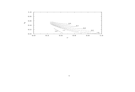
FIG. 6.: $F(\epsilon,\nu)$ as a function of $\nu$ at fixed $\epsilon$. Numbers near the curves show the values of $\epsilon$.

Our present data allow a rough estimate of the exponential suppression of the two-particle cross section in the region $E\sim E_{sph}$. This estimate can be obtained by extrapolating the function $F$ to $\nu=0$. Fig.6 shows the dependence of the function $F$ on $\nu$ for various values of $\epsilon$ in the range $\epsilon\sim 1$. Different curves of Fig.6 correspond to $\epsilon=0.6,0.7,0.8,0.9,1.0,1.1,2.0$ from top to bottom. The estimated value is

$\displaystyle F_{HG}(\epsilon=1)\approx 0.8$

with the accuracy of order 10%. Fig.6 confirms the conclusion that the dependence of $F_{HG}(\epsilon)$ on $\epsilon$ is slow: all curves, including the lowest one corresponding to $\epsilon=2$, converge as $\nu$ goes to zero and point roughly to the same value around $0.8$. One concludes that at $E\sim E_{sph}$ the zero energy instanton suppression is reduced by only about 20%. For more accurate estimate of the value of $F_{HG}(\epsilon)$ more data are needed in the region of small $\nu$.

VI Discussion and conclusions

Since no analogous calculations have been performed previously, it is worth to discuss in more detail the interpretation of the numerical results. The first point to be considered is their correspondence to the continuum theory. The algorithm we used in numerical calculations is asymmetric in $n_{t}$ and $n_{x}$; it mainly restricts the space grid resolution. So, the value of $n_{x}$ is our main concern.

FIG. 7.: Low energy perturbation theory for the periodic instanton ($\times$) versus numerical results at $n_{x}=80$ ($\diamond$) and $n_{x}=240$ (solid line) space points.

The results presented in the previous Section were obtained on the lattice with $n_{x}=80$ space points in the space volume $L=3m^{-1}$. In Fig.7 we plot the line of periodic instantons from Fig.5 (shown by diamonds) versus analytical expressions of Sect.4 (shown by crosses). The region of validity of perturbation theory does not overlap with $n_{x}=80$ data. Fortunately, in the case $\theta=0$ the grid resolution can be increased. In Fig.7 the solid line represents periodic instantons obtained numerically on the lattice with $n_{x}=240$ points. This line matches both the $n_{x}=80$ data and perturbation theory. It is clear from Fig.7 that $n_{x}=80$ data are accurate above $\nu=0.35$, at least in the case $\theta=0$. Fig.7 also indicates the region of validity of the perturbative results, eqs.(60)-(61).

FIG. 8.: Lines of constant $F$ at two grid resolutions: $n_{x}=80$ ($\diamond$) and $n_{x}=40$ (solid lines).

In the general case $\theta\neq 0$ we cannot match the perturbative and numerical results because we do not have numerical data at sufficiently small $\nu$ and $\epsilon$. In order to check the dependence on grid resolution, we plot in Fig.8 the $n_{x}=80$ data versus $n_{x}=40$ data of ref.[19]. The $n_{x}=40$ data are shown by solid lines. The agreement is good for $\nu\mathrel{\raisebox{-2.36806pt}{\hbox to0.0pt{$\sim$\hss}}\raisebox{1.72218pt}{$>$}}0.35$ and gets worse for smaller $\nu$, in accord with our previous estimate. The important observation is that the high-resolution curves lie above the low-resolution ones. Thus, both the exponential suppression of the two-particle cross section and the energy $E_{*}$ at which it may become exponentially unsuppressed are somewhat higher in the continuum limit than follows from our lattice results.

We turn now to the interpretation of the numerical solutions presented in Fig.5 as those describing the false vacuum decay. As mentioned in Sect.2, there may be several solutions to the boundary value problem (41); the physically relevant one is that continuously connected to the low energy periodic instanton. Since Fig.5 demonstrates perfectly smooth behavior and suggests the absence of bifurcations in the scanned region of parameters, we believe that the solutions of Fig.5 indeed describe the false vacuum decay. Here we consider more direct argument.

As explained in Sect.2, the real time part of each solution describes the evolution of the system after tunneling. By looking at the final field it is possible, in principle, to determine whether the false vacuum decay took place. In the model (48) the clear signature of the decay is a singularity of the field on the positive part of the real time axis (see Fig.9).

FIG. 9.: The position of singularities (shown by crossed circles) of the solution to the boundary value problem (41) in the $-\lambda\phi^{4}$ model. The boundary value problem is solved on the contour ABC.

Since the boundary value problem is solved on the contour ABC, the real time part of the solution has to be found separately by solving (numerically) the initial data problem along the real time axis, with initial values of the field and its time derivative determined by the solution on the contour ABC. We have performed such calculations and found that most of the solutions of Fig.5 indeed have singularity on the positive part of the real time axis, whereas some solutions, in particular those with $\epsilon\mathrel{\raisebox{-2.36806pt}{\hbox to0.0pt{$\sim$\hss}}\raisebox{1.72218pt}{$>$}}1.5$, apparently do not have such a singularity. There is, however, a problem with the interpretation of the results of this check. The reason is that the initial data problem mentioned above is unstable.

Let us consider the situation in more detail. As explained in Sect.2, the solutions to the boundary value problem (41) have specific analytic structure which requires the presence of singularity between the negative part of the real time axis and the contour ABC. In the model (48) this singularity lies at real negative time as shown in Fig.9. Since the boundary value problem is invariant under translations in the real time direction, only the distance between the two singularities of Fig.9 has invariant meaning. In numerical calculations the translational invariance is fixed by the constraint in such a way as to keep the left singularity at approximately the same place far from the asymptotic region A and not too close to the origin. All solutions of Fig.5 have left singularity in the range $-0.5<t<-0.3$.

As moving from left singularity of Fig.9 to the right one along the real time axis, the field comes from infinity, bounces off the potential barrier and goes back. At $E<E_{sph}$ this always takes finite amount of time. At $E>E_{sph}$ there exist solutions which spend long time oscillating above the sphaleron. Clearly, these solutions are unstable; small perturbations may cause them to roll finally to the false vacuum instead of going back to infinity. Numerical experiments show that the instability is very strong and gets worse for higher energies. Because of this instability, the position of the right singularity cannot be determined reliably when the distance to the singularity is larger than a certain amount, typically $\simeq 0.7$ for low energies and $\simeq 0.5$ for high energies. This can be checked by studying the dependence of the distance between the singularities on the constraint for given $E$ and $N$. When the constraint is imposed in such a way that the singularities are at the same distance from the origin, their positions are determined better. In the asymmetric case, the measured distance between singularities is always larger and the right singularity may even disappear.

At low energies and far from the line $F=0$, the distance between singularities is small enough to be determined reliably. In this region the right singularity is always present and the distance between the singularities does not depend on the constraint. At high energies or close to the line $F=0$, the distance is larger and becomes constraint–dependent, so that its real value cannot be determined by the above method. On the $(E-N)$ plane there is no well-defined boundary between the two regions. This makes us to infer that the interpretation of our solutions as describing the false vacuum decay is correct.

Let us come to conclusions. Numerical calculations we have performed demonstrate that the formalism of refs.[13, 14, 15] indeed provides a practical way to calculate the exponential suppression of the two-particle cross section of induced tunneling, $F_{HG}(\epsilon)$. The auxiliary object which we actually calculated, the logarithm of the multiparticle probability $F(\epsilon,\nu)$, has regular behavior consistent with theoretical expectations. This allows to set lower bounds on energy $E_{*}$ at which the two-particle cross section may become exponentially unsuppressed, and to estimate the value of the suppression at energies $E\sim E_{sph}$. We believe that analogous calculations are possible in any model with tunneling transitions.

In the $-\lambda\phi^{4}$ model we have found that the exponential suppression of the total cross section of induced false vacuum decay persists at least to energies of order $10E_{sph}$. At $E\sim E_{sph}$ about $80\%$ of the zero energy suppression is still present. The accuracy of this estimate crucially depends on the grid resolution, as can be seen from Fig.8.

Finally, let us comment on the similarity between the $-\lambda\phi^{4}$ model and the SU(2) Yang-Mills-Higgs system. It arises from the softly broken conformal symmetry present in both cases. Due to this (broken) symmetry, the low energy tunneling in both cases is dominated by constrained instantons whose size tends to zero in the limit $E\to 0$. The multiparticle rates should also have similar behavior, at least in the low energy domain. Therefore, we expect that in the SU(2) Yang-Mills-Higgs case it should be possible to calculate the function $F_{HG}(\epsilon)$ numerically along the lines we followed in this paper.

A Lattice formulation of the boundary value problem

In this Appendix we give the lattice formulation of the boundary value problem (41) and describe the method which we use to solve it.

We first note that the boundary value problem (41) is O(3)-symmetric, so we may restrict ourselves to field configurations depending on $r=\sqrt{\mbox{\boldmath$x$}^{2}}$ and $t$. In order to avoid the discretization of $r$–dependent derivative terms in the action, it is convenient to change variables according to

$\displaystyle\phi={1\over r}\psi.$

The action becomes

$$S=4\pi\int dt\int\limits_{0}^{\infty}dr\Bigl{\{}{1\over 2}{\dot{\psi}}^{2}-{1\over 2}(\partial_{r}\psi)^{2}-{1\over 2}\psi^{2}+{1\over 4r^{2}}\psi^{4}\Bigr{\}}.$$ (A1)

In order to obtain the lattice formulation of the boundary value problem (41), we first derive the lattice version of the exponent in eq.(14) and then repeat all steps of Sect.2 leading to eqs.(41).

Consider first the discretization of the action (A1). In the lattice formulation, it depends on ${(n_{t}+1)(n_{x}+1)}$ complex variables $\psi_{ij}=\psi(t_{i},r_{j})$, where $r_{i}\in[0,L]$ with $r_{0}=0$, $r_{n_{x}}=L$, while $t_{i}$ are complex numbers lying on the contour ABC of Fig.(9) so that $t_{0}=-T_{M}+iT/2$, $t_{n_{t}}=0$. When $T$ is small (this is the case in the high energy domain) the contour ABC passes close to the singularity of the field and the solution looses the accuracy. In this region of parameter space we deform the contour (leaving the point $t=0$ and the initial asymptotic region intact) so as to avoid the singularity.

Since fields are associated with the lattice sites while their derivatives are associated with links, we define two different sets of intervals

$\displaystyle dr_{j}=r_{j+1}-r_{j},\hskip 14.22636ptj=0\ldots n_{x}-1,$

and

$\displaystyle\tilde{dr_{j}}=(dr_{j-1}+dr_{j})/2,\hskip 14.22636ptj=1\ldots n_{x}-1,$

$\displaystyle\tilde{dr}_{0,n_{x}}=dr_{0,n_{x}-1}/2,$

and similarly for $dt_{i}$ and $\tilde{dt}_{i}$. The tilted intervals are used to approximate integrals with the integrand defined at lattice sites, while non-tilted ones are used for integrands defined on links. With these definitions, the discretized action (A1) reads

$$S = 4\pi\sum\limits_{ij}\Bigl{\{}{1\over 2}(\psi_{i+1,j}-\psi_{ij})^{2}{\tilde{dr_{j}}\over dt_{i}}$$ (A3)

$$-{1\over 2}(\psi_{i,j+1}-\psi_{ij})^{2}{\tilde{dt_{i}}\over dr_{j}}-V_{ij}\tilde{dt_{i}}\tilde{dr_{j}}\Bigr{\}},$$

where

$$V_{ij} = {1\over 2}\psi_{ij}^{2}-{1\over 4r_{j}^{2}}\psi_{ij}^{4}\;\;\;\mbox{at}\;\;\;j\neq 0,$$ (A4)

$$V_{i0} = 0\,.$$ (A5)

This discretization scheme has the advantage of being symmetric and additive: the action for the whole lattice is the sum of the actions of elementary plaquettes. It has the accuracy $O(dr^{2})$. The boundaries are treated to the same accuracy, which is important since the derivation of the boundary problem (41) requires integrations by parts.

Consider now the boundary term in eq.(14). On the lattice, the plane waves are no longer exact eigenfunctions of the Hamiltonian. To find their analog consider the quadratic part of eq.(A3) in the limit of continuous time,

$\displaystyle S^{(2)}=4\pi\int dt\sum\limits_{j}\Bigl{\{}{1\over 2}{\dot{\psi}_{j}}^{2}\tilde{dr_{j}}-{(\psi_{j+1}-\psi_{j})^{2}\over 2dr_{j}}-{1\over 2}\psi_{j}^{2}\tilde{dr_{j}}\Bigr{\}},$

where $\psi_{j}=\psi(t,r_{j})$. The kinetic term of this action takes the canonical form in terms of variables $\chi_{j}(t)=\psi_{j}(t)\sqrt{\tilde{dr_{j}}}$. The rest of the integrand can be written as minus free lattice Hamiltonian,

$\displaystyle-{1\over 2}\sum\limits_{jk}h_{jk}\chi_{j}\chi_{k},$

where

$$h_{jk} = \delta_{jk}\left({1\over\tilde{dr_{j}}dr_{j-1}}+{1\over\tilde{dr_{j}}dr_{j}}+1\right)$$ (A7)

$$-{\delta_{j+1,k}\over dr_{j}\sqrt{\tilde{dr_{j}}\tilde{dr_{k}}}}-{\delta_{j-1,k}\over dr_{k}\sqrt{\tilde{dr_{j}}\tilde{dr_{k}}}}.$$

The diagonalization of $h_{jk}$ determines the eigenfunctions $\xi^{(n)}_{k}$ and eigenvalues $\omega_{n}^{2}$ which substitute the plane waves and frequencies $\omega_{\bf k}^{2}$. We perform the diagonalization numerically. In fact, all expressions of Sect.2 involving momentum representation can be readily translated to the lattice language by means of the substitutions

$$\int d{\mbox{\boldmath$k$}} \to \sum\limits_{n}$$

$$\omega_{\bf k} \to \omega_{n}$$

$$\phi(t_{i},\mbox{\boldmath$k$}) \to \sum\limits_{j}\xi^{(n)}_{j}\sqrt{\tilde{dr_{j}}}\psi_{ij}.$$

In particular, the boundary term in eq.(39) becomes

$$\sum\limits_{jk}\Omega_{jk}\left\{-{1-\gamma\over 1+\gamma}\mathop{\mbox{Re}}\psi_{0j}\mathop{\mbox{Re}}\psi_{0k}+{1+\gamma\over 1-\gamma}\mathop{\mbox{Im}}\psi_{0j}\mathop{\mbox{Im}}\psi_{0k}\right\}$$ (A8)

where

$\displaystyle\Omega_{jk}=\sum\limits_{n}\sqrt{\tilde{dr_{j}}}\xi^{(n)}_{j}\omega_{n}\xi^{(n)}_{k}\sqrt{\tilde{dr_{k}}}.$

The matrix $\Omega_{jk}$ is calculated numerically. Note that it has to be calculated only once for a given spatial lattice $\{r_{j}\}$.

Now we are in position to derive the lattice version of the boundary value problem (41). The lattice analog of the field equation $\delta S/\delta\phi=0$ is

$$\frac{\partial S}{\partial\psi_{ij}}=0$$ (A9)

where $i=1...n_{t}-1$. The final boundary conditions immediately translate to

$$\mathop{\mbox{Im}}\psi_{n_{t},j} = 0,$$ (A10)

$$\mathop{\mbox{Im}}\frac{\partial S}{\partial\psi_{n_{t},j}} = 0.$$ (A11)

In order to derive the initial boundary conditions, one has to consider the lattice version of the exponent in eq.(14), take the derivative with respect to $\psi_{0j}$ and then set $\psi_{0j}^{\prime}=(\psi_{0j})^{*}$ and $\gamma_{\bf k}=\gamma=\mbox{e}^{-\theta}$ as discussed in Sect.2. The result reads

$$\frac{\partial S}{\partial\psi_{0j}}+\sum\limits_{k}\Omega_{jk}\left\{i{1-\gamma\over 1+\gamma}\mathop{\mbox{Re}}\psi_{0k}-{1+\gamma\over 1-\gamma}\mathop{\mbox{Im}}\psi_{0k}\right\}=0$$ (A12)

Note that total number of equations matches the number of unknowns. Eqs.(A9)-(A12) form a set of coupled non-linear algebraic equations which constitute the lattice analog of the boundary value problem (41).

As has been noted in Sect.5, in continuum version these equations are invariant under translation in the real time direction, which leads to the existence of almost zero mode on the lattice, i.e. continuous family of (approximate) solutions to eqs.(A9)-(A12). This spoils the convergence in the Newton-Raphson method and has to be cured. The standard trick is to introduce the constraint which breaks the translational invariance. In the vicinity of the sphaleron it is natural to require that at the point $t=0$ the field velocity has zero projection on the sphaleron negative mode,

$$\sum\limits_{j}\Xi_{j}^{(-)}\sqrt{\tilde{dr}_{j}}\frac{\partial S}{\partial\psi_{n_{t},j}}=0,$$ (A13)

where $\Xi_{j}^{(-)}$ is the sphaleron negative mode on the lattice. Far from the sphaleron there is no natural choice, so we use the constraint (A13) at all values of parameters. In the continuum theory physical quantities do not depend on the constraint.

B Numerical algorithm

Here we give basic formulae for the forward elimination – backward substitution algorithm which we use to solve the linear equations arising at each Newton-Raphson iteration.

The general form of the linearized equations is

$$L\cdot u=d,$$ (B1)

where $L$ is the matrix of first derivatives of the full equations, $u_{ij}$ are unknowns, while $-d_{ij}$ are full equations calculated at the current background ($d_{ij}=0$ if the background is a solution). The matrix $L$ has the dimension $(n_{t}+1)(n_{x}+1)\times(n_{t}+1)(n_{x}+1)$. It is a sparse matrix with a special structure which is most conveniently represented in the following form. Let us introduce vector notations in which the spatial index $j$ is implicit, $\mbox{\boldmath$u$}_{i}=\{u_{i0},\ldots,u_{in_{x}}\}$ and similarly for $\mbox{\boldmath$d$}_{i}$. Then the matrix $L$ has block-three-diagonal form with the diagonal blocks $\mbox{\boldmath$D$}_{i}$ and off-diagonal blocks $\mbox{\boldmath$D$}^{(-)}_{i}$ and $\mbox{\boldmath$D$}^{(+)}_{i}$, all of the same dimension $(n_{x}+1)\times(n_{x}+1)$. Eq.(B1) is equivalent to the following set of equations,

$$\begin{array}[]{lllllll}&&\mbox{\boldmath$D$}_{0}\mbox{\boldmath$u$}_{0}&+&\mbox{\boldmath$D$}^{(+)}_{0}\mbox{\boldmath$u$}_{1}&=&\mbox{\boldmath$d$}_{0},\\ &&&&&\ldots&\\ \mbox{\boldmath$D$}^{(-)}_{i}\mbox{\boldmath$u$}_{i-1}&+&\mbox{\boldmath$D$}_{i}\mbox{\boldmath$u$}_{i}&+&\mbox{\boldmath$D$}^{(+)}_{i}\mbox{\boldmath$u$}_{i+1}&=&\mbox{\boldmath$d$}_{i},\\ &&&&&\ldots&\\ \mbox{\boldmath$D$}^{(-)}_{n_{t}}\mbox{\boldmath$u$}_{n_{t}-1}&+&\mbox{\boldmath$D$}_{n_{t}}\mbox{\boldmath$u$}_{n_{t}}&&&=&\mbox{\boldmath$d$}_{n_{t}}.\end{array}$$ (B2)

The first and last of these equations represent the boundary conditions.

Let us define a set of matrices $\mbox{\boldmath$A$}_{i}$ of dimension $(n_{x}+1)\times(n_{x}+1)$ and vectors $\mbox{\boldmath$b$}_{i}$, $i=0\ldots n_{t}-1$, by the equations

$$\mbox{\boldmath$u$}_{i}=\mbox{\boldmath$A$}_{i}\mbox{\boldmath$u$}_{i+1}+\mbox{\boldmath$b$}_{i}.$$ (B3)

The first of eqs.(B2) implies

$\displaystyle\begin{array}[]{rcl}\mbox{\boldmath$A$}_{0}&=&-[\mbox{\boldmath$D$}_{0}]^{-1}\mbox{\boldmath$D$}^{(+)}_{0},\\ \mbox{\boldmath$b$}_{0}&=&[\mbox{\boldmath$D$}_{0}]^{-1}\mbox{\boldmath$d$}_{0}.\end{array}$

Eqs.(B2) and (B3) together give the recursion relation for $\mbox{\boldmath$A$}_{i}$ and $\mbox{\boldmath$b$}_{i}$,

$\displaystyle\begin{array}[]{rcl}\mbox{\boldmath$A$}_{i}&=&-[\mbox{\boldmath$D$}^{(-)}_{i}\mbox{\boldmath$A$}_{i-1}+\mbox{\boldmath$D$}_{i}]^{-1}\mbox{\boldmath$D$}^{(+)}_{i},\\ \mbox{\boldmath$b$}_{i}&=&[\mbox{\boldmath$D$}^{(-)}_{i}\mbox{\boldmath$A$}_{i-1}+\mbox{\boldmath$D$}_{i}]^{-1}[\mbox{\boldmath$d$}_{i}-\mbox{\boldmath$D$}^{(-)}_{i}\mbox{\boldmath$b$}_{i-1}].\end{array}$

At the stage of forward elimination, all $\mbox{\boldmath$A$}_{i}$ and $\mbox{\boldmath$b$}_{i}$ are calculated and stored (this procedure is equivalent to the elimination of the lower block-subdiagonal of the matrix $L$).

At the last point $i=n_{t}$, the third of eqs.(B2) and eq.(B3) taken at $i=n_{t}-1$ determine the vector of unknowns $\mbox{\boldmath$u$}_{n_{t}}$,

$\displaystyle\mbox{\boldmath$u$}_{n_{t}}=[\mbox{\boldmath$D$}^{(-)}_{n_{t}}\mbox{\boldmath$A$}_{n_{t}-1}+\mbox{\boldmath$D$}_{n_{t}}]^{-1}[\mbox{\boldmath$d$}_{n_{t}}-\mbox{\boldmath$D$}^{(-)}_{n_{t}}\mbox{\boldmath$b$}_{n_{t}-1}].$

Other unknowns are found by sequential use of eq.(B3) (back-substitution).

Clearly, the most time consuming stage is the calculation of the matrices $\mbox{\boldmath$A$}_{i}$. It amounts to matrix inversion and subsequent multiplication of the diagonal matrix by the result, all repeated $n_{t}$ times. This can be done in $\sim n_{t}n_{x}^{3}$ complex multiplications [27] with a coefficient close to 1. The algorithm requires storage space for $n_{t}n_{x}^{2}$ complex numbers.

REFERENCES

- [1] S. Coleman, Phys. Rev. D 15, 2929 (1977).
- [2] A. A. Belavin, A. M. Polyakov, A. S. Schwartz and Yu. S. Tyupkin, Phys. Lett. 59B, 85 (1975).
- [3] N. S. Manton, Phys. Rev. D 28, 2019 (1983); F. R. Klinkhamer and N. S. Manton, ibid. 30, 2212 (1984).
- [4] M. B. Voloshin, I. Yu. Kobzarev and L. B. Okun, Sov. J. Nucl. Phys. 20, 644 (1975).
- [5] A. Ringwald, Nucl. Phys. B330, 1 (1990); O. Espinosa, ibid. B334, 310 (1990).
- [6] G.’t Hooft, Phys. Rev. D 14, 3432 (1976).
- [7] V. A. Rubakov and M. E. Shaposhnikov, Usp. Fiz. Nauk 39, 461 (1996).
- [8] L. McLerran, A. Vainshtein and M. B. Voloshin, Phys. Rev. D 42, 171 (1990).
- [9] S. Yu. Khlebnikov, V. A. Rubakov and P. G. Tinyakov, Nucl. Phys. B350, 441 (1991).
- [10] L. Yaffe, Scattering amplitudes in instanton background, In: M. Mattis and E. Mottola, editors, Proceedings of the Santa Fe Workshop (World Scientific, Singapore, 1990).
- [11] P. B. Arnold and M. P. Mattis, Mod. Phys. Lett. A 6, 2059 (1991).
- [12] M. Mattis, Phys. Rep. 214, 159 (1992); P. G. Tinyakov, Int. J. Mod. Phys. A 8, 1823 (1993).
- [13] V. A. Rubakov and P. G. Tinyakov, Phys. Lett. B 279, 165 (1992).
- [14] P. G. Tinyakov, Phys. Lett. B 284, 410 (1992).
- [15] V. A. Rubakov, D. T. Son and P. G. Tinyakov, Phys. Lett. B 287, 342 (1992).
- [16] V. A. Rubakov and D. T. Son, Nucl. Phys. B422, 195 (1994); ibid. B424, 55 (1994).
- [17] I. K. Affleck and F. De Luccia, Phys. Rev. D 20, 3168 (1979); M. B. Voloshin and K. G. Selivanov, Yad. Fiz. 44, 1336 (1986); M. B. Voloshin, Nucl. Phys. B363, 425 (1991); J. Ellis, A. Linde and M. Sher, Phys. Lett. B 252, 203 (1990); V. A. Rubakov, D. T. Son and P. G. Tinyakov, Phys. Lett. B 278, 279 (1992).
- [18] V. I. Zakharov, Nucl. Phys. B353, 683 (1991); ibid. B383, 218 (1992).
- [19] A. N. Kuznetsov and P. G. Tinyakov, Mod. Phys. Lett. A 11, 479 (1996).
- [20] A. H. Mueller, Nucl. Phys. B401, 93 (1993).
- [21] L. D. Faddeev and A. A. Slavnov, Introduction to Quantum Theory of Gauge Fields (Nauka, Moscow, 1978).
- [22] C. Rebbi and R. Singleton, Phys. Rev. D 54, 1020 (1996).
- [23] S. Yu. Khlebnikov, V. A. Rubakov and P. G. Tinyakov, Nucl. Phys. B367, 334 (1991).
- [24] S. Fubini, Nuovo Cimento 34A, 521 (1976).
- [25] L. N. Lipatov, Zh. Eksp. Teor. Fiz. 72, 411 (1977).
- [26] I. Affleck, Nucl. Phys. B191, 455 (1981).
- [27] W. H. Press et al., Numerical Recipes in C (Cambridge University Press, England, 1992); R. Barrett et al., Templates for the Solution of Linear Systems: Building Blocks for Iterative Methods, (SIAM, Philadelphia, PA, 1994); C. C. Paige and M. A. Saunders, SIAM J. Numer. Anal. 12, 617 (1975); ACM Trans. Math. Soft. 8, 43 (1982).
- [28] M. Hellmund and J. Kripfganz, Nucl. Phys. B373, 749 (1992).
- [29] V. V. Matveev, Phys. Lett. B 304, 291 (1993).
- [30] S. Habib, E. Mottola and P. G. Tinyakov, Phys. Rev. D 54, 7774 (1996).