Semilocal string formation in two dimensions

Abstract

We present a toy model for the investigation of the formation of semilocal strings, where a planar symmetry is employed to reduce the system to two dimensions. We approximate the symmetry breaking using an extension of the Vachaspati–Vilenkin algorithm, where we throw down random phases for the scalar fields and then find the gauge field configuration which minimizes gradient energy in this fixed scalar background. We show this procedure reproduces the standard estimate for the formation rate of cosmic strings. For semilocal strings the configurations generated by this method are ambiguous, and we numerically evolve the configurations forward in time to identify which regions form strings. We find a significant rate of formation, depending on the ratio of couplings $\beta$. For low $\beta$ the formation rate is about one quarter that of cosmic strings; this falls as $\beta$ is increased and above $\beta=1$, where the string solution is dynamically unstable, no semilocal strings form. We show the results are robust by examining different initial conditions where, as expected in a thermal environment, the initial scalar field need not be on the vacuum. We discuss implications for the three-dimensional case.

]

I Introduction

As the universe expands and cools, one expects it to go through a variety of phase transitions. At each, there is the possibility of the formation of topological defects [2], the precise types being dictated by the physics of the breaking (see Ref. [3] for reviews). The standard examples are domain walls, cosmic strings, monopoles and texture, where for strings and monopoles one may have either a global or a local symmetry breaking. More recently, a new type of defect has been introduced which possesses both local and global symmetries, the simplest example being the semilocal string [4, 5].

Of great interest is the number density of defects which form. The standard technique for making such estimates is a discretization of space into correlation volumes, which may or may not be accompanied by a discretization of the vacuum manifold as well. This approach was pioneered by Vachaspati and Vilenkin [6] for the case of cosmic strings, and is easily generalized to monopoles, and, with a bit of further work, to global textures. These cases provide no particular difficulty because the presence or absence of defects is dictated solely by the configuration of the scalar field, regardless of whether the defects are global or local (though for global strings or monopoles the defect cores themselves prove not particularly important for the dynamics of the field ordering).

We wish to consider the formation of semilocal strings. This is a considerably harder problem, because the existence of string cores depends crucially on the way in which the scalar and gauge fields interact. The semilocal string scenario is characterized by the gauge fields having insufficient degrees of freedom to be able to completely cancel the scalar field gradients even away from the core of the string, and the final configuration depends very much on which of the gradients the gauge field chooses to cancel. Recently an analysis was made by Nagasawa and Yokoyama [7] for a related type of defect, the electroweak string [8] formed at the electroweak phase transition, using probabilistic arguments applied to thermal configurations. They concluded a very low production rate, though their analysis may significantly underestimate the extent to which configurations ‘near’ string configurations might relax to form proper strings since they do not consider the effect of the gauge fields in driving the Higgs values towards zero. Note also that such strings are unstable [9]. We adopt the alternative strategy of carrying out numerical simulations of initial configurations in order to determine those regions which prefer to accumulate magnetic flux to form strings. In this paper we shall only consider semilocal string formation in two dimensions, in order to test the method we propose. We shall turn to the three-dimensional case in a future publication. We specialize to two dimensions by imposing a planar symmetry.

We estimate the number density by an extension of the Vachaspati–Vilenkin algorithm [6]. First we generate an initial configuration by choosing a fixed scalar field background, upon which we find the gauge field configuration which minimizes the energy associated with the (covariant) gradients and magnetic field energy. Strings are identified by the location of flux tubes of Nielsen–Olesen type [10]. For cosmic strings we show that this accurately reproduces the standard result. For semilocal strings, however, the initial configurations thus generated are ambiguous, featuring a complicated structure of magnetic flux. We resolve this ambiguity by numerically evolving the configuration forward in time, allowing configurations in the ‘basin of attraction’ of the semilocal string solution to relax unambiguously into that configuration.

In order to confirm that our results are not an artifact of choosing particular initial conditions, we also carry out a set of simulations in which the scalar field is not initially on the vacuum manifold. In a truly thermal environment representing a second-order phase transition, one expects the field to be out of the vacuum as the phase transition completes, while the vacuum initial conditions are the expected outcome of a first-order phase transition. In any case, we find that the semilocal string density obtained in these simulations is extremely similar to that of the vacuum initial conditions.

II The Model

Semilocal strings arise in models with scalar fields and gauge fields, in which there are insufficient gauge degrees of freedom to completely cancel off the gradient energy associated with an inhomogeneous scalar field distribution [4]. The simplest such theory is one which contains two complex scalar fields coupled to a single abelian gauge field. Were there only one complex scalar field, one would have local cosmic strings, where the scalar gradients can be completely cancelled by the gauge field away from the string core. We shall use this standard situation as a test of our method.

The main question to be addressed in the formation of semilocal strings is which of the scalar gradients the gauge field chooses to cancel. As in any physical system, one expects the driving force will be the desire of the system to minimize its energy. We therefore propose the following model for determining conditions after the phase transition. First, we shall consider the scalar fields alone; when the symmetry breaks an independent choice of vacuum state is to be made in each correlation volume, in accordance with the Kibble mechanism [2]. At this point, the theory with two complex scalars is exactly that of a global texture theory. We then fix the scalar fields, and choose the gauge field to be in the configuration which minimizes the total energy in this fixed inhomogeneous scalar field background.

We work in flat space-time throughout. The Lagrangian for the simplest semilocal string model is

$${\cal L} = \left(\partial_{\mu}-iA_{\mu}\right)\phi_{1}^{\dagger}\left(\partial^{\mu}+iA^{\mu}\right)\phi_{1}$$ (3)

$$+\left(\partial_{\mu}-iA_{\mu}\right)\phi_{2}^{\dagger}\left(\partial^{\mu}+iA^{\mu}\right)\phi_{2}$$

$$-\frac{1}{4}F_{\mu\nu}F^{\mu\nu}-V(\phi_{1},\phi_{2})\,,$$

where $\phi_{1}$ and $\phi_{2}$ are two complex scalar fields, $A_{\mu}$ is the gauge field, the gauge coupling has been set to unity and $F_{\mu\nu}$ is the gauge field strength. The potential for the scalar fields is chosen to be of symmetry breaking type

$$V(\phi_{1},\phi_{2})=\frac{\beta}{2}\left(|\phi_{1}|^{2}+|\phi_{2}|^{2}-1\right)^{2}\,,$$ (4)

where the vacuum expectation value of the breaking, like the gauge coupling, has been scaled to unity as in Ref. [4]. The remaining parameter $\beta$, which cannot be scaled away, measures the relative strength of the scalar and gauge coupling constants (more specifically, $\beta\equiv m_{{\rm s}}^{2}/m_{{\rm v}}^{2}$ is the ratio between the squared scalar and vector masses). Its value determines the stability of an infinite semilocal string with a Nielsen–Olesen profile: the semilocal string is stable for $\beta<1$, neutrally stable for $\beta=1$ and unstable for $\beta>1$ [5, 11].

In this paper we shall only consider the two-dimensional situation obtained by imposition of a planar symmetry in the ‘3’ direction, $D_{3}\equiv 0$. Working in the gauge $A_{3}=0$, this reduces to the more familiar $\partial_{3}\equiv 0$. There is a residual gauge freedom which allows the further choice $A_{0}=0$. It is then clear that the energy-minimizing configurations will have $\partial_{0}=0$, since time derivatives appear quadratically. Splitting up the scalar fields into four real scalars via $\phi_{1}=\psi_{1}+i\psi_{2}$, $\phi_{2}=\psi_{3}+i\psi_{4}$, the energy density of a static configuration can be written

$$\rho = A_{1}^{2}+A_{2}^{2}+\frac{1}{2}\left(\partial_{1}A_{2}-\partial_{2}A_{1}\right)^{2}$$ (5)

$$- 2\left[A_{1}\psi_{1}\partial_{1}\psi_{2}-A_{1}\psi_{2}\partial_{1}\psi_{1}+A_{2}\psi_{1}\partial_{2}\psi_{2}-A_{2}\psi_{2}\partial_{2}\psi_{1}\right.$$ (7)

$$\left.\;+A_{1}\psi_{3}\partial_{1}\psi_{4}-A_{1}\psi_{4}\partial_{1}\psi_{3}+A_{2}\psi_{3}\partial_{2}\psi_{4}-A_{2}\psi_{4}\partial_{2}\psi_{3}\right]$$

$$+ \left(\partial_{1}\psi_{1}\right)^{2}+\left(\partial_{1}\psi_{2}\right)^{2}+\left(\partial_{1}\psi_{3}\right)^{2}+\left(\partial_{1}\psi_{4}\right)^{2}$$ (8)

$$+ \left(\partial_{2}\psi_{1}\right)^{2}+\left(\partial_{2}\psi_{2}\right)^{2}+\left(\partial_{2}\psi_{3}\right)^{2}+\left(\partial_{2}\psi_{4}\right)^{2}$$ (9)

$$+ V(\psi_{1},\psi_{2},\psi_{3},\psi_{4})\,.$$ (10)

Having thrown down the scalar field values and fixed them everywhere, the only terms required to minimize the energy are those depending on the remaining two components of the gauge field. This contribution to the energy density can be written as

$$\rho_{A}=A_{1}^{2}+A_{2}^{2}+2A_{1}f_{1}+2A_{2}f_{2}+\frac{1}{2}\left[\partial_{1}A_{2}-\partial_{2}A_{1}\right]^{2}\!\!,$$ (11)

where

$$f_{i}=-\psi_{1}\partial_{i}\psi_{2}+\psi_{2}\partial_{i}\psi_{1}-\psi_{3}\partial_{i}\psi_{4}+\psi_{4}\partial_{i}\psi_{3}\,,$$ (12)

gives the source terms for the gauge fields, which depend only on the (fixed) scalar field configuration. The remaining gauge terms are coupled only through the final magnetic flux term. Were it absent, there would be an analytic minimization of the energy given by

$$A_{1}({\bf x})=-f_{1}({\bf x})\quad;\quad A_{2}({\bf x})=-f_{2}({\bf x})\,.$$ (13)

This solution provides a good iterative starting point for finding the true minimum numerically, which will involve trading off some of the flux energy in the analytic solution for energy in the other terms. Consequently, the analytic solution provides an upper limit to the amount of flux energy possible in the minimum energy configuration.

III Initial Conditions and Evolution

A Initial conditions

There is no hope of an analytic minimization of Eq. (11) for a general scalar field configuration, so the problem must be dealt with via discretization. The problem being two-dimensional, we break up the space into a grid of dimension $N\times N$. The first stage is to lay down random phases for the scalar field to form the background for the energy minimization. The scalar field problem is just that of a global texture theory, which was examined in Ref. [12]. However, in that paper the vacuum manifold was discretized, which is unnecessary (and even disadvantageous) here; instead random locations on the vacuum manifold are chosen. Because the manifold has three-sphere topology, the scalar field can be in vacuum everywhere, in contrast to the usual cases where topology may force the scalar field to leave the vacuum manifold. However, once the gauge fields are introduced, they may make it energetically favourable for the scalar field to move away from the vacuum manifold, for example by allowing the magnetic flux to concentrate in areas of restored symmetry, and in such locations a semilocal string will have formed.

In order that the fields can be treated as fairly continuous on the grid, one should not throw down a completely random value at each grid-point. Instead, we choose the correlation length to be some number of grid-points and throw down phases on that coarser grid. The correlation length is chosen to be $2^{p}$ grid lengths, where $p$ is an integer. The field is then interpolated recursively onto the full grid by bisection. Thus our two-dimensional square grid with $2^{m}$ grid-points on a side contains $2^{2(m-p)}$ initial correlation volumes. Such a procedure was used in Ref. [13] to set up initial conditions for dynamical texture evolution. The simplest interpolation is somewhat discontinuous at the boundaries of the initial grid, which did not matter in Ref. [13] as they were quickly smoothed by dynamical evolution. Here we use a cubic interpolation in order to provide a smoother configuration that allow examination of the initial configuration itself. The gauge fields are subsequently chosen to minimize (covariant) gradients. We impose periodic boundary conditions; these enforce zero net flux through the grid, but this turns out to be unimportant provided the grid is sufficiently large.

We minimize the energy via a Monte Carlo procedure, starting with the analytic minimum Eq. (13), by choosing a grid-point and updating the gauge field values to new, energy-minimizing, values. After each point has been visited many times, the total energy is found to stabilize — we experimented with variation of the random sequence of points visited and also the initial conditions to confirm that the system did not get trapped in a false minimum.

This procedure is sufficient to obtain results for cosmic strings, reported in the next Section, simply by identifying visually (or automatically via a numerical analysis routine) the location of flux tubes in the configuration. For semilocal strings it proves impossible to decide from the iterated configuration which regions will become semilocal strings, as a very complex flux structure results due to the more complicated scalar field background. In order to resolve this ambiguity, it proves necessary to evolve the initial configuration forward in time to see what happens. It is also clear that this is necessary to distinguish the situations of stable and unstable semilocal strings, determined by the choice of $\beta$. The procedure thus far has been independent of $\beta$, but for $\beta>1$ we expect the flux to dissipate, while for $\beta<1$ some stable strings might form.

B Evolution

Both analytical [14, 15, 16] and numerical [11] methods have already been used to study issues concerned with stability of the string configurations for general $\beta$, and the cosmological implications, but have not been used to examine the evolution of initial configurations such as we have generated here.

With our gauge choices and with planar symmetry, the equations of motion from the Lagrangian of Eq. (3) are

$$\ddot{\psi}_{i}-\nabla^{2}\psi_{i}+\beta\left(\psi_{1}^{2}+\psi_{2}^{2}+\psi_{3}^{2}+\psi_{4}^{2}-1\right)\psi_{i}$$ (14)

$$\hskip 28.45274pt+A^{2}\psi_{i}+(-1)^{j}\left(2A.\nabla+\nabla.A\right)\psi_{j}=0\,,$$ (15)

(where $j$ is the complement of $i$ — $1\leftrightarrow 2$, $3\leftrightarrow 4$, and dots are of course time derivatives) for the scalar fields and

$$\ddot{A}_{i}-\nabla^{2}A_{i}+\partial_{i}\nabla.A+2\left(\psi_{1}\stackrel{{\scriptstyle\leftrightarrow}}{{\partial_{i}}}\psi_{2}+\psi_{3}\stackrel{{\scriptstyle\leftrightarrow}}{{\partial_{i}}}\psi_{4}\right)$$ (16)

$$+2A_{i}\left(\psi_{1}^{2}+\psi_{2}^{2}+\psi_{3}^{2}+\psi_{4}^{2}\right)=0\,,$$ (17)

for the gauge fields, together with the constraint (from the gauge choice)

$$2\left(\psi_{1}\stackrel{{\scriptstyle\leftrightarrow}}{{\partial_{0}}}\psi_{2}+\psi_{3}\stackrel{{\scriptstyle\leftrightarrow}}{{\partial_{0}}}\psi_{4}\right)+\partial_{i}\dot{A}_{i}=0\,,$$ (18)

which is used to test the stability of the code. The arrows indicate asymmetric derivatives.

This system is discretized using a standard staggered leapfrog method; however, to reduce its relaxation time we also add an ad hoc dissipation term to each equation — $\eta\dot{\psi}_{i}$ and $\eta\dot{A}_{i}$ respectively. In an expanding Universe the expansion rate would play such a role, though $\eta$ would typically not be constant. We tested a wide range of strengths of dissipation, and checked that it did not affect the end result, only the time the system took to adopt a distinctive structure. The simulations we display later used $\eta=0.5$. Fortunately we expect the long-range interactions between static parallel semilocal strings to be negligible [11] so we can take the number of flux tubes remaining at the end of the evolution to be a good estimate of the initial number of strings (and in any case a lower limit). This expectation is also borne out by examination of the flux tubes’ evolution over time.

IV Results

A Cosmic strings

To check our general strategy, we first test the performance of our codes for the case of cosmic strings. This simply involves ignoring one of the (complex) scalar fields, setting $\psi_{3}=\psi_{4}=0$. This makes the defects topological, and the flux tubes formed now map out the locations of winding in the scalar field configurations.

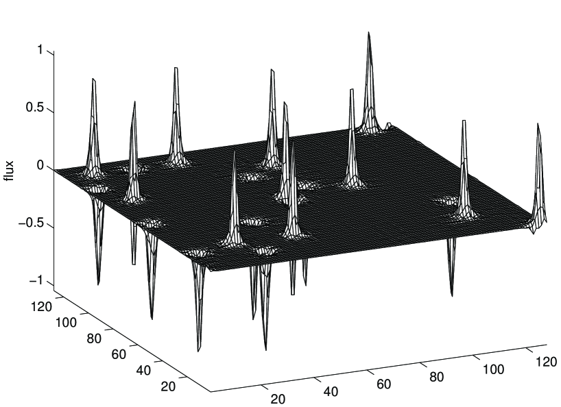
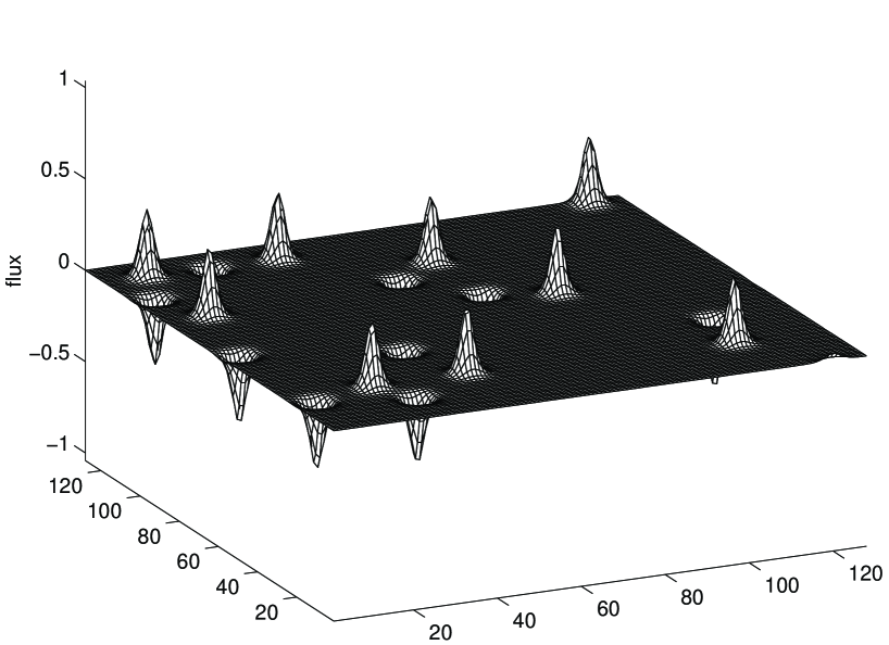
FIG. 1.: The flux tube structure of a cosmic string network. The flux tubes tend to line up on the sub-grid formed by the initial correlation length of 16 gridpoints. The spikes in the upper panel are taller and narrower than the corresponding Nielsen–Olesen vortices which result after evolution forward in time with $\beta=0.05$, as shown in the lower panel at $t=100$. Two flux pairs annihilate during this evolution.

In this case the flux tube structure is very well defined after the iteration has been used to produce the initial conditions, and we can directly estimate the number density of strings formed without needing any dynamical evolution. Using a $128^{2}$ grid and smoothing over every 16 grid-points we have 64 initial correlation volumes. An iterated configuration, with 22 flux tubes, is shown in the upper panel of Fig. 1. Examining 10 different initial field configurations we obtain a cosmic string number density

$$n_{{\rm cs}}=0.32\pm 0.02$$ (19)

per correlation volume. The error quoted is the standard error on the mean, but note that the uncertainty from discretization is somewhat larger.

This result agrees perfectly with the standard Vachaspati–Vilenkin algorithm on a 2-dimensional square lattice with a continuous field. Assuming the geodesic rule (i.e. that the field always covers the shortest path on the vacuum manifold along a grid edge), then the probability of string formation can be computed analytically. For example, take one corner to be at zero phase, take the diagonally opposite corner to be uniformly distributed in phase and compute the probability that the remaining two corners have phases in the right place to give a winding. The probability is given by

$$n_{{\rm cs}}^{{\rm VV}}=\frac{2}{(2\pi)^{3}}\int_{0}^{2\pi}(2\pi-\theta)\,\theta\,d\theta=\frac{1}{3}\,,$$ (20)

in agreement with what we found above. The good agreement arises because the simulations are themselves carried out on a square lattice, and confirms that our identification of cosmic strings via the flux tube structure works extremely well. The greatest uncertainty in the estimate comes from the choice of discretization; for example had we instead used a triangular lattice the Vachaspati–Vilenkin algorithm would give a formation rate of $1/4$ per triangle rather than $1/3$ per square [17], though one would also have to account for the difference in area.

Note that although the flux tubes in the upper panel of Fig. 1 are very clearly defined, they are not Nielsen–Olesen vortices [10], because the scalar field is everywhere in vacuum. Their width is governed by the inverse vector mass. Once the scalar fields are allowed to relax, the flux tubes become Nielsen–Olesen vortices. The result of dynamical evolution, for one hundred time units, is shown in the lower panel of Fig. 1, with $\beta$ chosen as 0.05. With that value, the inverse scalar mass is larger than the inverse vector mass (recall that $\beta\equiv m_{{\rm s}}^{2}/m_{{\rm v}}^{2}$) and so the total flux, while remaining $2\pi$, spreads over a larger area. During the evolution between the upper and lower panels, two pairs of flux tubes annihilate leaving 18 out of the original 22. Such annihilations are expected as the fields evolve and develop longer-range correlations, though this is inhibited by our artificial viscosity.

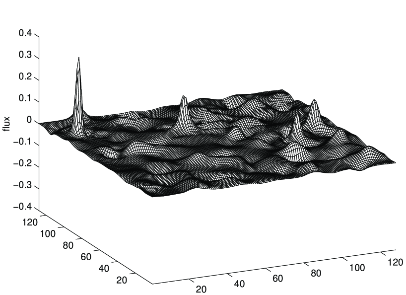
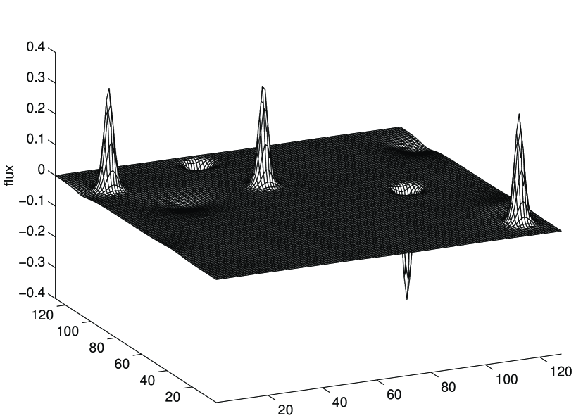
FIG. 2.: The flux tube structure in a semilocal string simulation. The upper panel ($t=0$) shows the initial condition after iteration, which is much more complicated than in the cosmic string case and not readily interpreted. The lower panel shows the configuration resolved into five flux tubes by a short period of dynamical evolution ($t=100$). Note that the vertical scale differs from that of Fig. 1; the final flux tubes have the same profile as in that case.

B Semilocal strings

For semilocal strings, the initial configurations generated by iteration prove much more ambiguous, because there is no topological constraint. One sees a complicated flux structure with extrema of different heights, and it is far from clear which of these, if any, might evolve to form semilocal strings; an example is shown in the top panel of Fig. 2. In any case, something has to be done to account for the influence of the parameter $\beta$, which determines the stability of the string configurations. We do this by evolving the system forward in time, including a dissipation term as described above to aid the relaxation. In fact, carrying out this dynamical evolution renders the energy-minimization process redundant, since the early stages of evolution carry out this role anyway.

As anticipated, in the unstable regime $\beta>1$ the flux quickly dissipates leaving no strings. In the stable regime $\beta<1$ stringlike features persist. The lower panel of Fig. 2 shows the result of evolving the configuration of the upper panel forward in time for one hundred time units (which is about a factor of two longer than the timescale found in Ref. [11] for the relaxation into semilocal strings of nearby configurations with non-zero winding number). Comparing the two panels indicates that some, but not all, of the more prominent flux features in the initial conditions do indeed relax into semilocal strings, that is, Nielsen–Olesen vortices identical to those shown in the bottom panel of Fig. 1 for the cosmic string case (note the different vertical scales of Figs. 1 and 2).

In order to automate the counting of flux tubes for the large number of simulations we have obtained, we adopt a criterion that any isolated extrenum in the magnetic flux which is at least half that of a perfect Neilsen–Olesen vortex is identified as a string. We tested this criterion on selected simulations which we studied in detail ourselves, and concluded it gives an accurate counting. This enabled us to carry out a large number of runs to bring down the statistical errors on our results.

For each of seven different values of $\beta$, we take 10 initial configurations on a $128^{2}$ grid smoothed over every $16$ grid-points. For $\beta<1$ we find a formation rate which depends on $\beta$, and which is always significant, though not as large as the number density found in the cosmic string case. At the smallest $\beta$ we were able to simulate, 0.05, the formation rate is about one quarter of that of cosmic strings. (If $\beta$ is lowered further, the scalar string cores become too wide to fit into a correlation volume.) Note that the lower number density means that annihilations during the early stages of evolution are less likely than in the cosmic string case, so would lead to an even smaller correction here.

FIG. 3.: The number of semilocal strings formed per initial correlation volume. Each point is an average over ten simulations. Squares indicate that the vacuum initial conditions of Section IV were used, while open circles indicate that the non-vacuum initial conditions described in Section V were used.

Support for our results comes from an analysis [11] in which simple configurations were permitted to relax into semilocal strings. It was found that configurations some way from a maximal circle (about one quarter of the way from the great circle for low values of $\beta$, decreasing to zero as $\beta$ approaches one) would relax into semilocal strings if $\beta<1$. Consider the values of the Higgs in four points on the lattice defining a grid square. All values lie on the three sphere. If we project all four points onto the most favourable maximal circle, then the probability of winding is identical to the Vachaspati–Vilenkin calculation, i.e. 1/3. Since the points are away from the maximal circle the suppression to the probability that they will still form a semilocal string can be estimated by whether the point which is furthest from the maximal circle is closer than a certain cutoff distance $D_{{\rm c}}$, and will be proportional to the volume of a fringe of width $2D_{{\rm c}}$ around the equator (over the total volume of the three sphere). Ref. [11] gives an estimate of $D_{{\rm c}}$, and the probability obtained is consistent with Fig. 3.

Notice that the final configuration illustrated in Fig. 2 does not have the same number of flux tubes of upward and downward pointing flux, despite the zero total flux boundary condition. The extra flux resides in small ‘nodules’ of flux that can be seen in the figure; although the maximum flux density is tiny, they are nevertheless quite diffuse and contain a significant amount of total flux. The structure of these nodules changes if the artificial viscosity is varied, indicating that they are in fact an artifact made long-lived by the viscous term. However, we note that if expansion was taken into account it would have some properties similar to our viscosity, and may permit such ‘skyrmionic’ configurations to be long-lived. Such a suggestion has been made by Benson and Bucher [16].

V Relaxing the initial conditions

In order to confirm the robustness of our conclusions, we also carried out the same number of simulations with different initial conditions. For a second-order phase transition, one expects the scalar field to be out of the vacuum as the transition takes place. This has been studied by Ye and Brandenberger [18], and we closely follow their strategy. They chose the scalar field magnitude randomly from a uniform distribution; we adopt a similar approach though using a gaussian distribution instead. We examined different choices for the width of the gaussian, and any reasonable choice makes no difference to the results. We shall display those for when the gaussian has a dispersion equal to the vacuum expectation value, which is the natural value at the phase transition.

We find startlingly good agreement with the vacuum initial conditions, as shown in Fig. 3. The same general shape for the $\beta$-dependence is found, and the number of strings identified per simulation is extremely close, with the error bars overlapping. For cosmic strings we found that the agreement between the two sets of simulations is not quite as good, though still impressive; some differences are expected as the initial correlation length will have changed, and we conclude that these changes are less significant for semilocal strings than cosmic strings.

VI Conclusions

In this paper we have proposed a method of investigating semilocal string formation by following the magnetic flux, and tested it by restricting the problem to two dimensions by imposing a planar symmetry. We have shown that our method can accurately reproduce the standard result for cosmic strings. We find a very significant rate of semilocal string formation; about one quarter the rate of cosmic string formation for the lowest $\beta$ we tested, falling towards zero as the unstable regime is reached at $\beta=1$. This result is robust to significant changes in the initial conditions.

Although superficially our result for the semilocal string density appears to be in disagreement with the very low probability of formation found by Nagasawa and Yokoyama for electroweak strings [7], a direct comparison cannot be made at this point. Their computation concerns the initial configuration only. It does not take into account the effect of the $A^{2}\phi^{2}$ term in the Lagrangian (which is usually responsible for the Meissner effect in superconductors), which will tend to drive the value of the Higgs field towards zero in regions where there is a high concentration of magnetic flux, in competition with the potential term which favours the vacuum value of the Higgs. Our simulations seem to indicate that the backreaction of the gauge fields is substantial, at least in the case of semilocal strings, and we expect this to be true also for electroweak strings as long as the SU(2) coupling is sufficiently small to allow stable strings. This may lead to string formation during the subsequent evolution. Further, the electroweak strings they consider are in fact unstable [9], and were we to carry out simulations of that case we would conclude a zero formation rate.

However, our simulations are only two-dimensional, and the three-dimensional implications are not straightforward. For cosmic strings, the two-dimensional formation rate can be used more or less directly to estimate the three-dimensional formation rate, because one can rely on the topology to ensure that the strings cannot end. Semilocal strings need not be infinite; there is the possibility that the strings might end in a diffuse cloud of flux resembling a global monopole. Further, the analytic infinite semilocal string solution corresponds to a winding of the gauge fields round a fixed great circle of the $S^{3}$ vacuum manifold, whereas in a realistic situation even if the winding condition continues to be obeyed as one moves along a putative string, the winding may correspond to different great circles at different points along the string and whether or not such a situation can be dynamically stable remains unexplored. Consequently, as yet we have no guidance as to how easily a configuration may find itself within a ‘basin of attraction’ of a semilocal string configuration. A complete picture of the formation rate must await full three-dimensional simulations, which are currently underway.

REFERENCES

- [1] Present addresses
- [2] T. W. B. Kibble, J. Phys. A9, 1387 (1976).
- [3] A. Vilenkin and E. P. S. Shellard, Cosmic Strings and Other Topological Defects, Cambridge University Press, Cambridge (1994); M. Hindmarsh and T. W. B. Kibble, Rep. Prog. Phys. 58, 477 (1995).
- [4] T. Vachaspati and A. Achúcarro, Phys. Rev D 44, 3067 (1991).
- [5] M. Hindmarsh, Phys. Rev. Lett. 68, 1263 (1992).
- [6] T. Vachaspati and A. Vilenkin, Phys. Rev D 30, 2036 (1984).
- [7] M. Nagasawa and J. Yokoyama, Phys. Rev. Lett. 77, 2166 (1996).
- [8] Y. Nambu, Nucl. Phys. B130, 505 (1977); T. Vachaspati, Phys. Rev. Lett. 68, 1977 (1992), (E) 69, 216 (1992), Nucl. Phys. B397, 648 (1993).
- [9] M. James, L. Perivolaropoulos and T. Vachaspati, Nucl. Phys. B395, 534 (1993); W. Perkins, Phys. Rev. D 47, R5224 (1993).
- [10] H. B. Nielsen and P. Olesen, Nucl. Phys. B61, 45 (1973).
- [11] A. Achúcarro, K. Kuijken, L. Perivolaropoulos and T. Vachaspati, Nucl. Phys. B388, 435 (1992).
- [12] J. Borrill, E. J. Copeland and A. R. Liddle, Phys. Lett. B258, 310 (1991).
- [13] J. Borrill, E. J. Copeland and A. R. Liddle, Phys. Rev. D 47, 4292 (1993).
- [14] J. Preskill, Phys. Rev. D 46, 4218 (1992); G. W. Gibbons, M. Ortiz, F. Ruiz-Ruiz and T. Samols, Nucl. Phys. B385, 127 (1992).
- [15] M. Hindmarsh, Nucl. Phys. B392, 461 (1993).
- [16] K. Benson and M. Bucher, Nucl. Phys. B406, 355 (1993).
- [17] R. Leese and T Prokopec, Phys. Rev. D 44, 3749 (1991); T. Prokopec, Phys. Lett. B 262, 215 (1991).
- [18] J. Ye and R. H. Brandenberger, Nucl. Phys. B346, 149 (1990).
- [19] P. M. Saffin and E. J. Copeland, Phys. Rev. D 56, 1215 (1997).