$W\gamma\gamma$ Production at the Fermilab Tevatron Collider: Gauge Invariance and Radiation Amplitude Zero

Abstract

The electroweak process $p\bar{p}\to\ell^{\pm}\nu\gamma\gamma$ is calculated at tree level, including finite $W$ width effects. In order to obtain a gauge invariant amplitude, the imaginary parts of $WW\gamma$ triangle graphs and $WW\gamma\gamma$ box diagrams have to be included, in addition to resumming the imaginary contributions to the $W$ vacuum polarization. We demonstrate the existence of a radiation amplitude zero in $p\bar{p}\rightarrow W^{\pm}\gamma\gamma\to\ell^{\pm}\nu\gamma\gamma$, and discuss how it may be observed in correlations of the $\gamma\gamma$ and lepton rapidities at the Fermilab Tevatron.

I Introduction

Radiative $W$ production and decay at hadron colliders is an important testing ground for the Standard Model (SM). The simplest process, $q\bar{q}^{\prime}\to\ell^{\pm}\nu\gamma$, allows the measurement of the $WW\gamma$ three gauge boson coupling at large photon transverse momenta [1, 2, 3, 4]. In addition, this process is of special interest due to the presence of a zero in the amplitude of the parton level process $q\bar{q}^{\prime}\to W\gamma$ [1, 5, 6]. At small transverse momenta of the photon or when the photon is emitted collinearly to the final state charged lepton, this process needs to be fully understood when trying to extract a precise value of the $W$ boson mass from Tevatron data. Approximately 24% (13%) of all $W\to e\nu$ ($W\to\mu\nu$) events contain a photon with a transverse momentum ($p_{T}^{\gamma}$) larger than 100 MeV [7, 8], the approximate threshold of the electromagnetic calorimeter of the CDF and DØ detectors. Radiative $W$ decay events shift the $W$ mass by about 65 MeV in the electron, and by approximately 170 MeV in the muon channel [9, 10].

For similar reasons, the process $q\bar{q}^{\prime}\to\ell^{\pm}\nu\gamma\gamma$ is interesting. At large photon transverse momenta, $W\gamma\gamma$ production is sensitive to the structure of the $WW\gamma\gamma$ quartic coupling [11]. Furthermore, as a consequence of a general theorem [6] one expects a radiation zero in the SM $q\bar{q}^{\prime}\to W\gamma\gamma$ amplitude. Two photon radiation is expected to have a non-negligible effect on the $W$ mass extracted from future high precision Tevatron data because approximately 0.8% of all $W\to\mu\nu$ events are expected to contain two well separated photons with $p_{T}^{\gamma}>100$ MeV [12]. Finally, $W\gamma\gamma$ production is an irreducible background to associated production of a $W$ and a Higgs boson in hadronic collisions, if the Higgs boson decays into two photons [13].

In $p\bar{p}$ collisions at a center of mass energy of 2 TeV, the total cross section for $W^{\pm}\gamma\gamma$ production is approximately 4.6 fb, when only considering leptonic decays, $W\to\ell\nu$ ($\ell=e,\,\mu$), and $p_{T}^{\gamma}>10$ GeV and $|\eta_{\gamma}|<2.5$ ($\eta$ being the pseudorapidity) [14]. Upgrades of the Tevatron accelerator complex (TeV33), beyond the Main Injector project, could yield an overall integrated luminosity of ${\cal O}(30$ fb^-1) [15], making a study of $W\gamma\gamma$ production a realistic goal in the TeV33 era. The hadronic decay modes of the $W$ will be difficult to observe due to the QCD $jj\gamma\gamma$ background [16]. We therefore concentrate on the leptonic decays of the $W$ boson, and calculate the helicity amplitudes for the complete process

$$q\bar{q}^{\prime}\to\ell^{\pm}\nu\gamma\gamma,$$ (1)

including Feynman diagrams where one or both photons are emitted from the final state charged lepton line. In a realistic simulation, these diagrams, together with finite $W$ width effects, need to be taken into account.

When including finite $W$ width effects, some care is needed to preserve gauge invariance. Replacing the $W$ propagator, $1/(q^{2}-m_{W}^{2})$, by a Breit-Wigner form, $1/(q^{2}-m_{W}^{2}+im_{W}\Gamma_{W})$, will disturb the gauge cancellations between the individual Feynman graphs and thus lead to an amplitude which is not electromagnetically gauge invariant. In addition, a constant imaginary part in the inverse propagator is ad hoc: it results from fermion loop contributions to the $W$ vacuum polarization and the imaginary part should vanish for space-like momentum transfers. In Ref. [8] it was demonstrated how this problem is solved for $W\gamma$ production by including the imaginary part of $WW\gamma$ vertex corrections in addition to the resummation of the $W$ vacuum polarization contributions. Here, we generalize the result of Ref. [8] to $W\gamma\gamma$ production, and show that a gauge invariant amplitude for the process $q\bar{q}^{\prime}\to\ell^{\pm}\nu\gamma\gamma$ is obtained by also including the imaginary part of the $WW\gamma\gamma$ box corrections. Extending the argument, a gauge invariant amplitude for $q\bar{q}^{\prime}\to W+n\gamma$, $n>2$, can be obtained by implementing the corrected $WW\gamma$ and $WW\gamma\gamma$ vertices together with the resummed $W$ vacuum polarization contributions. No higher $WWn\gamma$ vertex functions need to be considered. Our analysis of gauge invariance for $W\gamma\gamma$ production is described in Sec. II.

The existence of a radiation zero in the process $q\bar{q}^{\prime}\to W\gamma$ has been well known for more than fifteen years [5, 6]. All SM helicity amplitudes for the process $q\bar{q}^{\prime}\to W\gamma$ vanish at

$$\cos\theta^{*}_{W}=\cos\theta_{0W}^{*}=\frac{Q_{q}+Q_{q^{\prime}}}{Q_{q}-Q_{q^{\prime}}},$$ (2)

where $\theta^{*}_{W}$ is the angle between the $W$ and the incoming quark $q$, in the parton center of mass frame. A theorem [6] then predicts that the process $q\bar{q}^{\prime}\to W+n\gamma$, $n>1$, exhibits a radiation zero for the same scattering angle $\cos\theta_{0W}^{*}$, if the $n$ photons are collinear. In Sec. III, we numerically demonstrate the existence of this radiation zero in $W\gamma\gamma$ production.

In practice radiation zeros in hadronic collisions are difficult to observe. In the $W\gamma$ case, the ambiguity in reconstructing the parton center of mass frame and in identifying the quark momentum direction represents a major complication in the extraction of the $\cos\theta^{*}_{W}$ distribution [2]. Higher order QCD corrections [17, 18] and finite $W$ width effects, together with photon radiation from the final state lepton line, transform the zero to a dip [19]. Finite detector resolution effects further dilute the radiation zero. The twofold ambiguity in reconstructing the parton center of mass frame originates from the nonobservation of the neutrino arising from $W$ decay. Identifying the missing transverse energy with the transverse momentum of the neutrino, the unobservable longitudinal neutrino momentum, $p_{L}(\nu)$, and thus the parton center of mass frame, can be reconstructed by imposing the constraint that the neutrino and charged lepton four momenta combine to form the $W$ rest mass [20]. The resulting quadratic equation, in general, has two solutions. Finally, determining the $\cos\theta^{*}_{W}$ distribution requires measurement of the missing transverse energy in the event. In future Tevatron runs, one expects up to ten interactions per bunch crossing [15]. Multiple interactions per crossing significantly worsen the missing transverse energy resolution, and thus tend to wash out the dip caused by the radiation zero.

For $W\gamma\gamma$ production, the same problems arise. In addition, it is very difficult to experimentally separate two collinear photons, and, thus, to distinguish the $W\gamma\gamma$ signal from $W\gamma$ events and from the $W+$ jets background, where one of the jets fluctuates into a $\pi^{0}$ which decays into two almost collinear photons. One therefore has to search for a signal of the radiation zero which survives an explicit photon–photon separation requirement.

In Ref. [21] it was found that lepton–photon rapidity correlations offer the best chance to observe the radiation zero in $W\gamma$ production. The distribution of the rapidity difference $\Delta y(\gamma,\ell)=y_{\gamma}-y_{\ell}$ clearly displays the SM radiation zero. It does not require knowledge of the longitudinal momentum of the neutrino, and so automatically avoids the problems described above. In Sec. III we show that the concept of rapidity correlations as a tool to search for radiation zeros can be generalized to the $W\gamma\gamma$ case. The $\Delta y(\gamma\gamma,\ell)$ distribution with $\cos\theta_{\gamma\gamma}>0$, where $\theta_{\gamma\gamma}$ is the opening angle between the two photons in the laboratory system, clearly displays the SM radiation zero even when one requires two well separated photons, provided that cuts are imposed which reduce the background from radiative $W$ decays.

It is sometimes useful to compare distributions for $W\gamma\gamma$ and $Z\gamma\gamma$ production. Simultaneously with the calculation of the process $q\bar{q}^{\prime}\to\ell^{\pm}\nu\gamma\gamma$, we therefore also present results for $q\bar{q}\to\ell^{+}\ell^{-}\gamma\gamma$ production in Sec. III. Section IV contains some concluding remarks.

II Finite Width Effects and Gauge Invariance in $W\gamma\gamma$ Production

At the parton level, the reaction $p\bar{p}\to\ell^{\pm}\nu\gamma\gamma$ proceeds via the Feynman diagrams shown in Fig. 1. Besides the diagrams for $W\gamma\gamma$ production, graphs describing $W\gamma$ production followed by $W\to\ell\nu\gamma$ contribute, and also the radiative decay $W\to\ell\nu\gamma\gamma$. When finite $W$ width effects are included, the three reactions can no longer be distinguished, and the full set of Feynman diagrams must be taken into account. To calculate the helicity amplitudes for the process $q\bar{q}^{\prime}\to\ell^{\pm}\nu\gamma\gamma$ we have used the framework of Refs. [22] and [23]. The result was then compared numerically with the amplitudes obtained using the MADGRAPH/HELAS program [24, 25] which generates helicity amplitudes automatically. All quarks and leptons were assumed to be massless in our numerical calculations.

FIG. 1.: Feynman diagrams for the process $q\bar{q}^{\prime}\to\ell\nu\gamma\gamma$. Permutations of the final state photons and the $W$ boson are not shown explicitly.

A naive implementation of finite $W$ width effects, by replacing the $W$ propagator by a Breit–Wigner form with momentum dependent width, leads to a violation of electromagnetic gauge invariance [26] and the resulting cross sections cannot be trusted. One encounters the same problem when gauge invariance is restored in an ad hoc manner [8, 27]. Finite width effects are included in a tree level calculation by resumming the imaginary part of the $W$ vacuum polarization. Gauge boson loops ($W\gamma$ and $WZ$) only contribute above the $W$-mass pole and are suppressed by threshold factors [28]. They can safely be neglected at the desired level of accuracy and only fermion loops need to be considered. Neglecting the fermion masses in the loops, the transverse part of the $W$ vacuum polarization receives an imaginary contribution

$$Im\,\Pi_{W}^{T}(q^{2})=\sum_{f}{g^{2}\over 48\pi}q^{2}=q^{2}{\Gamma_{W}\over m_{W}}=q^{2}\gamma_{W}\;,$$ (3)

while the imaginary part of the longitudinal piece vanishes. In the unitary gauge the $W$ propagator is thus given by

$$D_{W}^{\mu\nu}(q) = {-i\over q^{2}-m_{W}^{2}+iIm\,\Pi_{W}^{T}(q^{2})}\left(g^{\mu\nu}-{q^{\mu}q^{\nu}\over q^{2}}\right)+{i\over m_{W}^{2}-iIm\,\Pi_{W}^{L}(q^{2})}\;{q^{\mu}q^{\nu}\over q^{2}}$$ (4)

$$= {-i\over q^{2}-m_{W}^{2}+iq^{2}\gamma_{W}}\left(g^{\mu\nu}-{q^{\mu}q^{\nu}\over m_{W}^{2}}(1+i\gamma_{W})\right)\;.$$ (5)

A gauge invariant expression for the amplitude of the process $q\bar{q}^{\prime}\to\ell^{\pm}\nu\gamma\gamma$ is obtained by attaching the final state photons in all possible ways to all charged particle propagators in the Feynman graphs. To be specific, we shall concentrate on the $\ell^{-}\bar{\nu}\gamma\gamma$ final state in the following. In addition to radiation off the external fermion lines and radiation off the $W$ propagators, the photons must be attached to the charged fermions inside the $W$ vacuum polarization loops, leading to the fermion triangle and box graphs of Figs. 2 and 3. Since we are only keeping the imaginary part of $\Pi_{W}^{T}(q^{2})$, consistency requires including the imaginary parts of the triangle and box graphs only. These imaginary parts are obtained by cutting the triangle and box graphs into on-shell intermediate states in all possible ways, as shown in the figures.

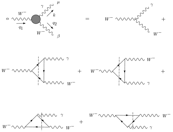
FIG. 2.: The effective $WW\gamma$ vertex as needed in the tree level calculation of $\ell\nu\gamma\gamma$ production.

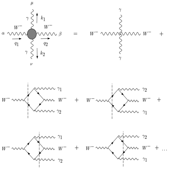
FIG. 3.: The Feynman graphs contributing to the effective $WW\gamma\gamma$ vertex of Eq. (9). Only four of the 24 cut box diagrams which contribute to the imaginary part of the one-loop $WW\gamma\gamma$ vertex are shown.

For the momentum flow displayed in Figs. 2 and 3, the tree level $WW\gamma$ and $WW\gamma\gamma$ vertices are given by the familiar expressions

$$-ie\Gamma_{0}^{\alpha\beta\mu} = -ie\left((q_{1}+q_{2})^{\mu}g^{\alpha\beta}-(q_{1}+k)^{\beta}g^{\mu\alpha}+(k-q_{2})^{\alpha}g^{\mu\beta}\right)\;,$$ (6)

$$-ie\Gamma_{0}^{\alpha\beta\mu\nu} = -ie^{2}\left(2g^{\alpha\beta}g^{\mu\nu}-g^{\alpha\mu}g^{\beta\nu}-g^{\alpha\nu}g^{\beta\mu}\right)\;.$$ (7)

For the triangle graphs of Fig. 2 the momentum configuration, $q_{1}^{2}>q_{2}^{2},\;k^{2}=0$, is the same as the one encountered in the $q\bar{q}^{\prime}\to\ell^{\pm}\nu\gamma$ case. Neglecting fermion masses, the full $WW\gamma$ vertex is then given by [8]

$$\Gamma^{\alpha\beta\mu}=\Gamma_{0}^{\alpha\beta\mu}\left(1+\sum_{f}{ig^{2}\over 48\pi}\right)=\Gamma_{0}^{\alpha\beta\mu}\left(1+i\,{\Gamma_{W}\over m_{W}}\right)=\Gamma_{0}^{\alpha\beta\mu}\left(1+i\gamma_{W}\right)\;.$$ (8)

Non-zero fermion masses, $m_{f}>0$, introduce corrections to Eq. (8) and generate axial vector contributions to the $WW\gamma$ vertex which are proportional to $m_{f}^{2}/q_{1}^{2}$ and $m_{f}^{2}/q_{2}^{2}$ [29]. They can be neglected at the desired level of accuracy for the lepton and the light quark doublets. Top-bottom loops do not contribute to the imaginary part of the $WW\gamma$ vertex below threshold, i.e. for $q_{i}^{2}<(m_{t}+m_{b})^{2}$. In the imaginary part of the $WW\gamma\gamma$ vertex they are either absent for $q_{i}^{2}<(m_{t}+m_{b})^{2}$ or are suppressed by powers of the top quark mass. These massive loops are not needed for the restoration of electromagnetic gauge invariance and can be neglected close to the $W$ pole.

An evaluation of the 24 cut box diagrams of Fig. 3 yields a result similar to that of Eq. (8) [30]. For vanishing fermion masses, each fermion doublet $f$, irrespective of its hypercharge, adds $i(g^{2}/48\pi)\Gamma_{0}^{\alpha\beta\mu\nu}$ to the tree level $WW\gamma\gamma$ vertex $\Gamma_{0}^{\alpha\beta\mu\nu}$. In the phase space region $q_{1}^{2}>q_{2}^{2},\;k_{1}^{2}=k_{2}^{2}=0$, the full $WW\gamma\gamma$ vertex is thus given by

$$\Gamma^{\alpha\beta\mu\nu}=\Gamma_{0}^{\alpha\beta\mu\nu}\left(1+i\gamma_{W}\right)\;.$$ (9)

In the expressions for the two vertices, terms proportional to $k_{1}^{\mu}$ or $k_{2}^{\nu}$ have been dropped. Such terms will be contracted with the photon polarization vectors $\varepsilon^{*\mu}(k_{1})$ or $\varepsilon^{*\nu}(k_{2})$, or a conserved electromagnetic current and hence vanish in the amplitude. Similarly, terms proportional to $q_{1}^{\alpha}$ are dropped since, in the massless quark limit, the $W$ couples to a conserved quark current. No such assumption is made for the $W$-decay leptons, and hence our expressions are valid when including finite charged lepton masses. For off-shell photons or space-like $W$-bosons, more complicated expressions are obtained [31].

By construction, the resulting amplitude for the process $q\bar{q}^{\prime}\to\ell^{-}\bar{\nu}\gamma\gamma$ should be gauge invariant. Indeed, gauge invariance of the full amplitude can be traced to the electromagnetic Ward identities

$$k_{\mu}{\Gamma_{\alpha\beta}}^{\mu}=\left(iD_{W}\right)^{-1}_{\alpha\beta}(q_{1})-\left(iD_{W}\right)^{-1}_{\alpha\beta}(q_{2})\;,$$ (10)

between the $WW\gamma$ vertex and the inverse $W$ propagator [26] and

$$k_{1}^{\mu}\Gamma_{\alpha\beta\mu\nu}(q_{1},q_{2},k_{1},k_{2})=e\left(\Gamma_{\alpha\beta\nu}(q_{1},q_{2}+k_{1},k_{2})-\Gamma_{\alpha\beta\nu}(q_{1}-k_{1},q_{2},k_{2})\right)\;,$$ (11)

relating three- and four-point functions. Since

$$k_{\mu}\Gamma^{\alpha\beta\mu}=\left((q_{1}^{2}g^{\alpha\beta}-q_{1}^{\alpha}q_{1}^{\beta})-(q_{2}^{2}g^{\alpha\beta}-q_{2}^{\alpha}q_{2}^{\beta})\right)\left(1+i\gamma_{W}\right)\;,$$ (12)

and

$$\left(iD_{W}\right)^{-1}_{\alpha\beta}(q)=\left(q^{2}-m_{W}^{2}+iq^{2}\gamma_{W}\right)\left(g_{\alpha\beta}-{q_{\alpha}q_{\beta}\over q^{2}}\right)-m_{W}^{2}{q_{\alpha}q_{\beta}\over q^{2}}\;,$$ (13)

the Ward identity of Eq. (10) is satisfied for the $W$ propagator and $WW\gamma$ vertex of Eqs. (5) and (8). Similarly the Ward identity for the $WW\gamma\gamma$ vertex is verified for the explicit three- and four-point functions of Eqs. (8) and (9).

Extending this analysis to the $WW\gamma\gamma\gamma$ vertex, the relevant Ward identity relating $WW\gamma\gamma\gamma$- and $WW\gamma\gamma$ vertices is given by

$$k_{1\mu}\Gamma_{\alpha\beta\nu\rho}^{\mu}(q_{1},q_{2},k_{1},k_{2},k_{3})=e\left(\Gamma_{\alpha\beta\nu\rho}(q_{1},q_{2}+k_{1},k_{2},k_{3})-\Gamma_{\alpha\beta\nu\rho}(q_{1}-k_{1},q_{2},k_{2},k_{3})\right)\;.$$ (14)

The right hand side vanishes for the tree-level $WW\gamma\gamma$ vertex and thus also for the fermion-one-loop corrected vertex of Eq. (9). This means that the amplitude for the three photon process $q\bar{q}^{\prime}\to\ell^{\pm}\nu\gamma\gamma\gamma$ is rendered gauge invariant by implementing the corrected $WW\gamma$ and $WW\gamma\gamma$ vertex functions only, but without taking into account any $WW\gamma\gamma\gamma$ one-loop correction. The argument can immediately be generalized to an arbitrary number of final state photons. For hard, non-collinear photon emission this is mostly of theoretical interest, however, since the cross section for $W\gamma\gamma\gamma$ production, already, is expected to be too small to be observed even at a high luminosity Tevatron.

Returning to the calculation of the $q\bar{q}^{\prime}\to\ell\nu\gamma\gamma$ amplitude, a gauge invariant result is obtained by replacing all $W$-propagators, $WW\gamma$ and $WW\gamma\gamma$ vertices in the Feynman graphs of Fig. 1 by the full expressions of Eqs. (5), (8) and (9), respectively. Formally, these expressions include the imaginary parts of up to two loops in the vertices of Fig. 1(e). However, the Dyson resummation of the $W$-propagators already constitutes a mixing of all orders of perturbation theory and thus the appearance of several vertex loops should be no surprise. This result is obtained naturally by attaching the two photons in all possible ways to either one of the fermion loops or to one of the lowest order $W$ propagators in the zero, one, two etc. fermion bubble graphs contributing to the Dyson resummed process $q\bar{q}^{\prime}\to\ell\nu$: the remaining sum over $W$ vacuum polarization graphs restores the full $W$ propagator of Eq. (5) on either side of a triangle graph, a $WW\gamma$ vertex, the box graph, or the $WW\gamma\gamma$ vertex. After resummation, one therefore obtains the Feynman graphs of Fig. 1 where any $WW\gamma(\gamma)$ vertex is given by the sum of the lowest order vertex and the imaginary part of the triangle (box) graphs, as defined in Figs. 2 and 3.

Finally note that conservation of the final state lepton current has not been assumed anywhere, i.e. terms proportional to $q_{2}^{\beta}$ have been kept throughout. Thus our calculation is correct for massive final state leptons and the emission of two photons collinear with the charged final state lepton can be simulated with the resulting code [12]. Alternative approaches in treating unstable gauge bosons in a gauge invariant way have been discussed in Ref. [32].

III Searching for the Radiation Zero in $W\gamma\gamma$ Production at the Tevatron

A Input Parameters and Detector Simulation

We now study in detail the radiation zero in $q\bar{q}^{\prime}\to W\gamma\gamma$ predicted by the SM, for $p\bar{p}$ collisions at $\sqrt{s}=2$ TeV. To simplify the discussion, we shall concentrate on the $W^{-}\gamma\gamma$, $W^{-}\to e^{-}\bar{\nu}$ channel. In $p\bar{p}$ collisions, the total cross sections for $W^{-}\gamma\gamma$ and $W^{+}\gamma\gamma$ production are equal. Angular and rapidity distributions for the $W^{+}$ case can be obtained by a sign change of the variable. The parameters used in our numerical simulations are $m_{W}=80.22$ GeV, $m_{Z}=91.187$ GeV, and $\alpha_{em}=1/128$. We use the parton distribution functions set A of Martin-Roberts-Stirling [33] with the factorization scale set equal to the parton center of mass energy, $\sqrt{\hat{s}}$.

To simulate the finite acceptance of detectors, we impose cuts on observable particles in the final state. Unless otherwise stated, we require:

$$p_{T}^{\gamma} > 10\ {\rm GeV},\quad|y_{\gamma}|<2.5,\quad\Delta R_{\gamma\gamma}>0.3\quad{\rm for\ photons},$$ (15)

$$p_{T}^{e} > 15\ {\rm GeV},\quad|y_{e}|<2.5,\quad\Delta R_{e\gamma}>0.7\quad{\rm for\ charged\ leptons},$$ (16)

and

$$p\hbox to0.0pt{\hss/}_{T}>15~{}{\rm GeV}.$$ (17)

Here, $p_{T}$ is the transverse momentum and $y$ the rapidity of a particle, and $p\hbox to0.0pt{\hss/}_{T}$ denotes the missing transverse momentum of the event, defined by the imbalance to $p_{T}^{e}$ and $p_{T}^{\gamma}$ in our calculation. For massless particles, the rapidity and the pseudorapidity, $\eta$, coincide.

$$\Delta R=\sqrt{(\Delta\phi)^{2}+(\Delta\eta)^{2}}$$ (18)

denotes the separation in the pseudorapidity–azimuthal angle plane. Without finite $p_{T}^{\gamma}$ and $\Delta R_{e\gamma}$ cuts, the cross section for $e\nu\gamma\gamma$ production would diverge, due to the various collinear and infrared singularities present.

As mentioned in the Introduction, it is instructive to compare the results obtained for $q\bar{q}^{\prime}\to e^{-}\nu\gamma\gamma$ with those for the neutral channel, $q\bar{q}\to e^{+}e^{-}\gamma\gamma$. In this case, we also impose a

$$M(e^{+}e^{-})>20\ {\rm GeV}$$ (19)

cut to avoid the mass singularity from timelike virtual photon exchange graphs. The $q\bar{q}\to e^{+}e^{-}\gamma\gamma$ helicity amplitudes were calculated using the same technique which we employed in the $e\nu\gamma\gamma$ case. The transverse momentum and rapidity cuts listed above approximate the phase-space region which will be covered by the upgraded CDF [34] and DØ detectors [35].

Uncertainties in the energy measurement of electrons and photons are, unless stated otherwise, taken into account in our numerical simulations by Gaussian smearing with

$${\sigma\over E}={0.2\over\sqrt{E}}\oplus 0.01\;,$$ (20)

where the two terms are added in quadrature and $E$ is in units of GeV. The only visible effect of the finite energy resolution in the figures presented below arises in regions of phase space where the cross section changes very rapidly, e.g. around the $W$ or $Z$ boson peaks.

For the cuts listed in Eq. (15), backgrounds to $e\nu\gamma\gamma$ and $e^{+}e^{-}\gamma\gamma$ production are small, provided the two photons are well isolated from any hadronic energy in the event. The isolation cut essentially eliminates the backgrounds from $W\gamma+1$ jet and $W+2$ jet production where one or both jets fragment into a photon [36]. For $p_{T}^{\gamma}>10$ GeV, the probability that a jet fakes a photon, $P_{j/\gamma}$, is $10^{-3}$ or less [4]. Backgrounds from $W\gamma+$ jets and $W+$ jets production, where one or two jets fake a photon, are then small. The photon-photon separation cut of $\Delta R_{\gamma\gamma}>0.3$, combined with a substantial $p_{T}^{\gamma}$, requires a sizable invariant mass of the two-photon system and thereby eliminates backgrounds from $\pi^{0}\to\gamma\gamma$ decays which might originate from $W/Z+1$ jet production with a leading $\pi^{0}$.

The geometrical acceptance of the upgraded CDF and DØ detectors for muons will be similar to that for electrons. Requiring the charged lepton to be well separated from the photons, the cross sections for $e\nu\gamma\gamma$ and $\mu\nu\gamma\gamma$ production are then nearly identical. The results derived in the following for the electron channel therefore also apply to the $\mu\nu\gamma\gamma$ final state.

B The $e^{-}\bar{\nu}\gamma\gamma$ and $W^{-}(\to e^{-}\bar{\nu})\gamma\gamma$ Cross Sections

In Fig. 4, we present the total cross sections, within the cuts of Sec. IIIA, for $p\bar{p}\rightarrow e^{-}\bar{\nu}\gamma\gamma$ and on-shell $W^{-}(\to e^{-}\bar{\nu})\gamma\gamma$ production (solid) as a function of the $p\bar{p}$ center of mass energy. For comparison, we also show the cross sections for $e^{+}e^{-}\gamma\gamma$ and $Z(\to e^{+}e^{-})\gamma\gamma$ production (dashed). Here the on-shell $W^{-}(\to e^{-}\bar{\nu})\gamma\gamma$ and $Z(\to e^{+}e^{-})\gamma\gamma$ cross sections have been calculated in the narrow $W/Z$ width approximations. The large differences between the on-shell and the full cross sections arise from diagrams where one or both photons are emitted by a final state charged lepton. For $e^{+}e^{-}\gamma\gamma$ events there are also sizable contributions from $\gamma^{*}\to e^{+}e^{-}$. Contributions from these diagrams increase the cross section by about a factor 3 (6) in the $W\gamma\gamma$ ($Z\gamma\gamma$) case for the cuts chosen. No energy smearing effects are taken into account in Fig. 4.

FIG. 4.: The total cross sections for $p\bar{p}\to e^{-}\bar{\nu}\gamma\gamma$ and $p\bar{p}\to W^{-}(\to e^{-}\bar{\nu})\gamma\gamma$ (solid lines) as a function of the $p\bar{p}$ center of mass energy, $\sqrt{s}$. For comparison, we also show the $p\bar{p}\to e^{+}e^{-}\gamma\gamma$ and $p\bar{p}\to Z(\to e^{+}e^{-})\gamma\gamma$ cross sections (dashed lines). The acceptance cuts are summarized in Sec. IIIA. No energy smearing is imposed.

The rates for $p\bar{p}\to W^{-}(\to e^{-}\bar{\nu})\gamma\gamma$ and $p\bar{p}\to Z(\to e^{+}e^{-})\gamma\gamma$ [14] are almost identical over the entire center of mass range studied for the cuts chosen. This should be contrasted with the cross section ratio of $W^{-}(\to e^{-}\bar{\nu})+2$ jet to $Z(\to e^{+}e^{-})+2$ jet production which is about 4.6 [37]. The relative suppression of the $W\gamma\gamma$ cross section can be traced to the radiation zero which is present in $W\gamma\gamma$, but not in $Z\gamma\gamma$ production. Similarly, the $W\gamma$ cross section is suppressed relative to the $Z\gamma$ production rate because of the radiation zero in $q\bar{q}^{\prime}\to W\gamma$ [38].

Figure 4 shows that, although we require the charged lepton to be well separated from the photons, radiation off the final state charged lepton completely dominates. In order to search for a possible radiation zero in $W\gamma\gamma$ production, it is necessary to suppress final state bremsstrahlung more efficiently. To isolate the $W(\to e\nu)\gamma\gamma$ component in $p\bar{p}\to e\nu\gamma\gamma$, it is useful to study the transverse mass distribution of the $e\nu$ system which is shown in Fig. 5(a). $W(\to e\nu)\gamma\gamma$ events produce a $M_{T}(e\nu)$ distribution which is sharply peaked at $M_{T}(e\nu)=m_{W}$. However, finite energy resolution effects significantly dilute this peak (see solid curve). On the other hand, if one or both photons are emitted by the charged lepton, the $e\nu$ transverse mass tends to be considerably smaller than the $W$ mass. Requiring

$$M_{T}(e^{-}\nu)>70~{}{\rm GeV,}$$ (21)

eliminates most of the contributions from final state radiation. With this additional cut, the total and differential cross sections for $e\nu\gamma\gamma$ and $W(\to e\nu)\gamma\gamma$ production are almost identical.

FIG. 5.: (a) The ${e\nu}$ transverse mass distribution for ${p\bar{p}\to e^{-}\bar{\nu}\gamma\gamma}$, and (b) the ${e^{+}e^{-}}$ invariant mass distribution for ${p\bar{p}\to e^{+}e^{-}\gamma\gamma}$, at ${\sqrt{s}=2}$ TeV. The cuts imposed are summarized in Sec. IIIA. The solid and dotted curves give the results with and without taking into account the finite energy resolution of detectors (see Eq. (20)).

Similarly, a cut on the di-lepton invariant mass can be used to suppress photon radiation from the final state leptons in $p\bar{p}\to e^{+}e^{-}\gamma\gamma$. The $e^{+}e^{-}$ invariant mass distribution, for the cuts summarized in Sec. IIIA, is shown in Fig. 5(b). The two broad peaks below the $Z$ resonance region correspond to contributions from $Z\rightarrow e^{+}e^{-}\gamma$ and $Z\rightarrow e^{+}e^{-}\gamma\gamma$. Details of the structure depend on the choices of $p_{T}^{\gamma}$ and $\Delta R_{e\gamma}$ cuts. For

$$M(e^{+}e^{-})>85~{}{\rm GeV,}$$ (22)

contributions from final state bremsstrahlung are reduced by about a factor of 4 for $p_{T}^{\gamma}>10$ GeV. Nevertheless, contributions from final state bremsstrahlung and $\gamma^{*}\to e^{+}e^{-}$ are still sizeable in this case.

Within the cuts of Eqs. (15) and (17), and with the transverse mass cut of $M_{T}(\ell\nu)>70$ GeV, the total $\ell^{\pm}\nu\gamma\gamma$ ($\ell=e,\,\mu$) cross section for $p\bar{p}$ collisions at $\sqrt{s}=2$ TeV is about 2 fb. For an integrated luminosity of 30 fb^-1, one thus expects about 60 $\ell^{\pm}\nu\gamma\gamma$ events. The cross section depends quite sensitively on the minimum photon transverse momentum, $p_{T}^{\rm min}$, however. This dependence, with and without the transverse mass cut of Eq. (21), is shown in Fig. 6 for the $e^{-}\bar{\nu}\gamma\gamma$ cross section. For completeness, curves for $p\bar{p}\to e^{+}e^{-}\gamma\gamma$ are included as well. No energy smearing effects are taken into account here. Reducing the photon transverse momentum threshold from 10 GeV to 4 GeV, the $e^{-}\bar{\nu}\gamma\gamma$ rate, regardless of the transverse mass cut of Eq. (21), increases by about a factor of 6. Due to the limited number of $e\nu\gamma\gamma$ events even at the highest Tevatron luminosities, the $p_{T}$ threshold for at least one of the photons should be lowered as far as possible in a search for the radiation zero in $W\gamma\gamma$ production. Nevertheless, in our further analysis, we shall retain the more stringent photon transverse momentum requirement of $p_{T}^{\gamma}>10$ GeV for both photons (see Eq. (15)). As mentioned in Sec. IIIA, backgrounds from $W\gamma+$ jets and $W+$ jets production, where one or two jets fake a photon, are then small. Furthermore, we shall impose the mass cuts of Eq. (21) and (22) unless stated otherwise.

FIG. 6.: The total cross sections for $p\bar{p}\rightarrow e^{-}\bar{\nu}\gamma\gamma$ and $p\bar{p}\to e^{+}e^{-}\gamma\gamma$ at $\sqrt{s}=2$ TeV as a function of the minimal photon transverse momentum $p_{T}^{\rm min}$. The solid lines are for the cuts summarized in Sec. IIIA. For the dashed lines an additional $M_{T}(e\nu)>70$ GeV or $M(e^{+}e^{-})>85$ GeV cut has been imposed. No energy smearing is included here.

C Searching for the Radiation Zero

The general theorem of Ref. [6] states that, in the SM, the amplitude for the process $d\bar{u}\to W^{-}\gamma\gamma$ vanishes for

$$\cos\theta_{W}^{*}=\cos\theta_{0W^{-}}^{*}=\frac{Q_{d}+Q_{u}}{Q_{d}-Q_{u}}=-{1\over 3},$$ (23)

FIG. 7.: The angular distribution of the vector boson for the partonic processes (a) $d\bar{u}\rightarrow W^{-}\gamma\gamma$ with $M_{\gamma\gamma}=0$, and (b) $d\bar{u}\rightarrow W^{-}\gamma$, at $\sqrt{\hat{s}}=300$ GeV (solid lines). Corresponding curves for $u\bar{u}\to Z\gamma\gamma$ and $u\bar{u}\to Z\gamma$ (dashed lines) are also shown for comparison. The photon energies in the $W\gamma\gamma$ and $Z\gamma\gamma$ case are chosen to be equal. The differential cross sections are in arbitrary units. No cuts and no energy smearing are imposed, and the $W$ and $Z$ bosons are treated as stable particles.

when the two photons are collinear. Here $\theta_{W}^{*}$ is the angle between the incoming $d$-quark and the $W$ boson, and the asterisk on a quantity denotes that it is to be taken in the parton center of mass frame. For $W^{+}\gamma\gamma$ production, the role of the $u$- and $d$-quarks in Eq. (23) are interchanged, i.e. $\cos\theta_{0W^{+}}^{*}=-\cos\theta_{0W^{-}}^{*}$. The existence of the radiation zero can be readily verified numerically. Figure 7(a) shows the $\cos\theta_{W}^{*}$ distribution for the parton level process $d\bar{u}\to W^{-}\gamma\gamma$, at a parton center of mass energy of $\sqrt{\hat{s}}=300$ GeV and for $M_{\gamma\gamma}=0$, which forces the two photons to be collinear. In addition, the photon energies are chosen to be equal. For unequal photon energies, qualitatively very similar results are obtained. The vanishing of the differential cross section at $\cos\theta_{0W^{-}}^{*}=-1/3$ is apparent. For comparison, we have also included the $\cos\theta_{Z}^{*}$ distribution for $u\bar{u}\to Z\gamma\gamma$ in Fig. 7(a) (dashed line), and show the $\cos\theta_{W}^{*}$ and $\cos\theta_{Z}^{*}$ distributions for $d\bar{u}\to W^{-}\gamma$ and $u\bar{u}\to Z\gamma$ at $\sqrt{\hat{s}}=300$ GeV in Fig. 7(b). The $\cos\theta_{W}^{*}$ region where the cross section is substantially reduced due to the zero is seen to be considerably larger in the $W\gamma\gamma$ case. No cuts and no energy smearing have been imposed in Fig. 7, and the $W$ and $Z$ bosons are treated as stable particles. The overall normalization of the cross sections in each part of the figure is arbitrary. Similar results are obtained for different parton center of mass energies.

The impressive $W\gamma\gamma$ radiation zero in Fig. 7 is washed out by the small contamination of $W(\to e^{-}\bar{\nu}\gamma)\gamma$ and $W\to e^{-}\bar{\nu}\gamma\gamma$ events which pass the $M_{T}(e^{-}\bar{\nu})$ cut of Eq. (21) when $W$ decays and finite $W$ width effects are taken into account. Binning effects reduce the radiation zero to a mere dip as well. This is shown in Fig. 8 where we display the normalized double differential cross section $(1/\hat{\sigma})(d^{2}\hat{\sigma}/d\cos\theta_{W}^{*}\,d\cos\theta^{*}_{\gamma\gamma})$ for the partonic process $d\bar{u}\to e^{-}\bar{\nu}\gamma\gamma$ with $\sqrt{\hat{s}}=300$ GeV. Here $\theta^{*}_{\gamma\gamma}$ is the angle between the two photons in the parton center of mass frame. In this figure, the full set of contributing Feynman diagrams, including the corrections to the $W$ propagator and the $WW\gamma$ and $WW\gamma\gamma$ vertices described in Sec. II, have been taken into account, together with the cuts summarized in Eqs. (15), (17) and (21) which we subsequently impose in all figures.

Figure 8 demonstrates that the dip in the $e^{-}\bar{\nu}\gamma\gamma$ differential cross section at $\cos\theta^{*}_{W}=-1/3$, which signals the presence of the $W\gamma\gamma$ radiation zero, is quite pronounced for the cuts we have chosen. It also shows that it only gradually vanishes for increasing values of $\theta^{*}_{\gamma\gamma}$. Requiring two photons with $\Delta R_{\gamma\gamma}>0.3$ therefore has no significant effect on the observability of the $W\gamma\gamma$ radiation zero.

FIG. 8.: The normalized double differential distribution $(1/\hat{\sigma})\,(d^{2}\hat{\sigma}/d\cos\theta^{*}_{\gamma\gamma}\,d\cos\theta^{*}_{W})$ for the partonic process $d\bar{u}\to e^{-}\bar{\nu}\gamma\gamma$ at ${\sqrt{\hat{s}}=300}$ GeV. The cuts summarized in Eqs. (15), (17) and (21) are imposed.

The significance of the dip, which signals the amplitude zero, is potentially further reduced by the convolution with parton distribution functions and by the twofold ambiguity in reconstructing the parton center of mass frame. This twofold ambiguity originates from the non-observation of the neutrino arising from $W$ decay. Setting the $e\nu$ invariant mass equal to $m_{W}$ leaves two solutions for the reconstructed center of mass, which can be ordered according to whether the rapidity of the neutrino is larger (“plus” solution) or smaller (“minus” solution) than the rapidity of the electron [2]. Since the photons couple more strongly to the incoming up-type anti-quark, the $W^{-}$ boson tends to be emitted in the proton direction. Within the SM, and as in $W\gamma$ production, the dominant helicity of the $W^{-}$ boson in $W\gamma\gamma$ production is $\lambda_{W}=-1$, implying that the electron is more likely to be emitted in the direction of the parent $W$. The rapidity of the electron thus is typically larger than that of the neutrino, and the “minus” solution better preserves the dip caused by the radiation zero. In $W^{+}\gamma\gamma$ production, the $W$ boson is dominantly emitted into the $\bar{p}$ direction, and, consequently, the “plus” solution shows more similarity with the true reconstructed parton center of mass.

The normalized double differential distribution $(1/\sigma)\,(d^{2}\sigma/d\cos\theta^{*}_{\gamma\gamma}\,d\cos\theta^{*}_{W})$ for the process $p\bar{p}\to e^{-}\bar{\nu}\gamma\gamma$ at $\sqrt{s}=2$ TeV is shown in Fig. 9, using the “minus” solution for the reconstructed parton center of mass. The distribution is seen to be quite similar to the corresponding partonic differential cross section shown in Fig. 8. The convolution with the parton distribution functions therefore has only a minor effect on the observability of the radiation zero. Likewise, the reconstruction of the parton center of mass frame does not affect the significance of the dip much, provided that the appropriate solution for the longitudinal momentum of the neutrino is used, and the missing transverse momentum is well measured (see below).

FIG. 9.: The normalized double differential distribution $(1/\sigma)\,(d^{2}\sigma/d\cos\theta^{*}_{\gamma\gamma}\,d\cos\theta^{*}_{W})$ for the process $p\bar{p}\to e^{-}\bar{\nu}\gamma\gamma$ at ${\sqrt{s}=2}$ TeV, using the “minus” solution for the reconstructed parton center of mass. The cuts summarized in Eqs. (15), (17) and (21) are imposed.

For the limited number of $e\nu\gamma\gamma$ events expected in future Tevatron runs, it will be impossible to map out the double differential distribution shown in Fig. 9. However, since the dip signaling the radiation zero disappears only gradually with increasing values of $\theta^{*}_{\gamma\gamma}$, most of the information present in $d^{2}\sigma/d\cos\theta^{*}_{\gamma\gamma}\,d\cos\theta^{*}_{W}$ is contained in the $\cos\theta^{*}_{W}$ distributions for events with $\cos\theta^{*}_{\gamma\gamma}>0$ versus $\cos\theta^{*}_{\gamma\gamma}<0$. These two $\cos\theta^{*}_{W}$ distributions are shown in Fig. 10, for both the “plus” and the “minus” solution of the reconstructed parton center of mass frame. For comparison, Fig. 10 also shows the $\cos\theta^{*}_{Z}$ distribution for $p\bar{p}\to e^{+}e^{-}\gamma\gamma$ with $M(e^{+}e^{-})>85$ GeV and the cuts of Eq. (15). For $\cos\theta^{*}_{\gamma\gamma}>0$ and using the “minus” solution, the $\cos\theta^{*}_{W}$ distribution displays a pronounced dip located at $\cos\theta^{*}_{W}\approx-1/3$. For the “plus” solution the minimum is shifted to $\cos\theta^{*}_{W}\approx 0$. In contrast, requiring $\cos\theta^{*}_{\gamma\gamma}<0$, the dip is drastically reduced, and the differential cross section at $\cos\theta^{*}_{W}\approx-1/3$ is about one order of magnitude larger than for $\cos\theta^{*}_{\gamma\gamma}>0$ (see Fig. 10(b)). The large difference in the $\cos\theta^{*}_{W}$ distribution for $\cos\theta^{*}_{\gamma\gamma}>0$ and $\cos\theta^{*}_{\gamma\gamma}<0$ becomes more apparent by comparing the $\cos\theta^{*}_{Z}$ distribution in $Z\gamma\gamma$ production in the two regions. Unlike the situation encountered in $W\gamma\gamma$ production, the $\cos\theta^{*}_{Z}$ distributions for $\cos\theta^{*}_{\gamma\gamma}>0$ and $\cos\theta^{*}_{\gamma\gamma}<0$ are very similar.

FIG. 10.: The $\cos\theta^{*}_{W}$ distribution for $p\bar{p}\to e^{-}\bar{\nu}\gamma\gamma$ at ${\sqrt{s}=2}$ TeV, for (a) $\cos\theta^{*}_{\gamma\gamma}>0$ and (b) $\cos\theta^{*}_{\gamma\gamma}<0$. The solid (dashed) line is for the “minus” (“plus”) solution of the reconstructed parton center of mass frame. The dotted line displays the $\cos\theta_{Z}^{*}$ distribution for $p\bar{p}\to e^{+}e^{-}\gamma\gamma$ for comparison. The cuts summarized in Eqs. (15), (17) and (21) are imposed. In the $Z\gamma\gamma$ case, the cuts listed in Eqs. (15) and (22) are applied.

Determining the $\cos\theta^{*}_{W}$ distribution requires measurement of the transverse momentum of the neutrino produced in the $W$ decay. In $e\nu\gamma\gamma$ production, the neutrino transverse momentum is identified with the missing transverse energy, $E\hbox to0.0pt{\hss/}_{T}$, in the event. In future Tevatron runs, one expects up to ten interactions per bunch crossing [15]. Multiple interactions per crossing significantly worsen the $E\hbox to0.0pt{\hss/}_{T}$ resolution, and thus tend to wash out the dip signaling the radiation zero. We have not included missing transverse energy resolution effects in our simulations, since the number of interactions per crossing, and hence the $E\hbox to0.0pt{\hss/}_{T}$ resolution, sensitively depend on the future Tevatron accelerator parameters which are difficult to foresee at present.

Due to the negative impact of multiple interactions on the missing transverse energy resolution, it is advantageous to search for a kinematic variable which exhibits a clear signal of the radiation zero but does not depend on the neutrino momentum. The $y_{\gamma\gamma}-y_{e}$ distribution is a possible candidate for such a variable. Here $y_{e}$ is the electron rapidity and $y_{\gamma\gamma}$ denotes the rapidity of the two-photon system in the laboratory frame.

In Ref. [21] it was found that photon lepton rapidity correlations are a useful tool to search for the radiation zero in $W\gamma$ production. The distribution of the rapidity difference, $\Delta y(\gamma,e)=y_{\gamma}-y_{e}$, which does not require knowledge of the missing transverse energy or the longitudinal momentum of the neutrino, clearly displays the SM radiation zero in form of a dip. In the parton center of mass frame, the photon and $W$ boson in $q\bar{q}^{\prime}\to W^{-}\gamma$ are back to back. Due to the radiation zero, the photon and $W$ rapidity distributions in the parton center of mass frame, $d\sigma/dy^{*}_{\gamma}$ and $d\sigma/dy^{*}_{W}$, display pronounced dips located at

$$y^{*}_{\gamma} = {1\over 2}\ln 2\approx 0.35,$$ (24)

$$y^{*}_{W} \approx -0.05.$$ (25)

If $W$ mass effects could be ignored, one would expect that $y^{*}_{\gamma}=-y^{*}_{W}$. Since differences of rapidities are invariant under longitudinal boosts, the difference of the photon and the $W$ rapidity in the laboratory frame then exhibits a dip at

$$\Delta y(\gamma,W)=y_{\gamma}-y_{W}=y^{*}_{\gamma}-y^{*}_{W}\approx 0.4.$$ (26)

As discussed earlier, the dominant $W$ helicity in $W^{\pm}\gamma$ production is $\lambda_{W}=\pm 1$, implying that the charged lepton tends to be emitted in the direction of the parent $W$, and thus reflects most of its kinematic properties. The dip signaling the presence of the radiation zero therefore manifests itself in the $\Delta y(\gamma,\ell)$ distribution. Since the average rapidity of the lepton and the $W$ are slightly different, the location of the minimum is shifted to $\Delta y(\gamma,\ell)\approx 0.1$.

The radiation zero in $W\gamma\gamma$ production occurs at exactly the same rapidity as the zero in $W\gamma$ production, when the photons are collinear. One therefore expects that the $\Delta y(\gamma\gamma,W)$ distribution displays a clear dip for photons with a small opening angle, $\theta_{\gamma\gamma}$, in the laboratory frame, i.e. at $\cos\theta_{\gamma\gamma}\approx 1$. In Fig. 11 we show the double differential distribution $d^{2}\sigma/d\cos\theta_{\gamma\gamma}\,d(y_{\gamma\gamma}-y_{W})$, using the “minus” solution for the longitudinal neutrino momentum. For $\Delta y(\gamma\gamma,W)\approx 0.4$, a clear dip is visible for $\cos\theta_{\gamma\gamma}$ values close to one. The dip gradually vanishes for larger opening angles between the two photons, leading to a “canyon” in the double differential distribution. Due to the finite invariant mass of the $\gamma\gamma$ system for non-zero values of $\theta_{\gamma\gamma}$, the location of the minimum in $\Delta y(\gamma\gamma,W)$ varies slightly with $\cos\theta_{\gamma\gamma}$.

FIG. 11.: The double differential distribution $d^{2}\sigma/d\cos\theta_{\gamma\gamma}\,d(y_{\gamma\gamma}-y_{W})$ for the process $p\bar{p}\to e^{-}\bar{\nu}\gamma\gamma$ at ${\sqrt{s}=2}$ TeV, using the “minus” solution for the longitudinal neutrino momentum. The cuts summarized in Eqs. (15), (17) and (21) are imposed.

Since the dip vanishes gradually with decreasing $\cos\theta_{\gamma\gamma}$, it is useful to consider the $\Delta y(\gamma\gamma,W)$ distribution for $\cos\theta_{\gamma\gamma}>0$ and $\cos\theta_{\gamma\gamma}<0$. Figure 12(a) displays a pronounced dip in $d\sigma/d\Delta y(\gamma\gamma,W)$ for $\cos\theta_{\gamma\gamma}>0$, located at $\Delta y(\gamma\gamma,W)\approx 0.7$ (solid line). In contrast, for $\cos\theta_{\gamma\gamma}<0$, the $\Delta y(\gamma\gamma,W)$ distribution does not exhibit a dip (dashed line). The $\Delta y(\gamma\gamma,W)$ distribution for $\cos\theta_{\gamma\gamma}>0$ thus plays a role similar to the $\Delta y(\gamma,W)$ distribution in $W\gamma$ production. In the dip region, the differential cross section for $\cos\theta_{\gamma\gamma}<0$ is about one order of magnitude larger than for $\cos\theta_{\gamma\gamma}>0$. In addition, the $\Delta y(\gamma\gamma,W)$ distribution extends to significantly higher $y_{\gamma\gamma}-y_{W}$ values if one requires $\cos\theta_{\gamma\gamma}>0$. This reflects the narrower rapidity distribution of the two-photon system for $\cos\theta_{\gamma\gamma}<0$, due to the larger invariant mass of the system when the two photons are well separated.

FIG. 12.: Rapidity difference distributions for $p\bar{p}\to e^{-}\bar{\nu}\gamma\gamma$ at ${\sqrt{s}=2}$ TeV. Part (a) shows the $y_{\gamma\gamma}-y_{W}$ spectrum, while part (b) displays the $y_{\gamma\gamma}-y_{e}$ distribution. The solid (dashed) curves are for $\cos\theta_{\gamma\gamma}>0$ ($\cos\theta_{\gamma\gamma}<0$). The cuts summarized in Eqs. (15), (17) and (21) are imposed.

Exactly as in the $W\gamma$ case, the dominant helicity of the $W$ boson in $W^{\pm}\gamma\gamma$ production is $\lambda_{W}=\pm 1$. One therefore expects that the distribution of the rapidity difference of the $\gamma\gamma$ system and the electron is very similar to the $y_{\gamma\gamma}-y_{W}$ distribution and shows a clear signal of the radiation zero for positive values of $\cos\theta_{\gamma\gamma}$. The $y_{\gamma\gamma}-y_{e}$ distribution, shown in Fig. 12(b), indeed clearly displays these features. Due to the finite difference between the electron and the $W$ rapidities, the location of the minimum is again slightly shifted. The $\Delta R_{\gamma\gamma}>0.3$ cut has only little effect on the significance of the dip.

The characteristic differences between the $\Delta y(\gamma\gamma,e)=y_{\gamma\gamma}-y_{e}$ distribution for $\cos\theta_{\gamma\gamma}>0$ and $\cos\theta_{\gamma\gamma}<0$ are also reflected in the cross section ratio

$${\cal R}={\int_{\Delta y(\gamma\gamma,e)>-1}d\sigma\over\int_{\Delta y(\gamma\gamma,e)<-1}d\sigma}~{},$$ (27)

which may be useful for small event samples. Many experimental uncertainties cancel in ${\cal R}$. For $\cos\theta_{\gamma\gamma}>0$ one finds ${\cal R}\approx 0.25$, whereas for $\cos\theta_{\gamma\gamma}<0$ ${\cal R}\approx 1.06$.

Our calculations have all been carried out in the Born approximation. The complete NLO QCD corrections to $W\gamma\gamma$ production have not been calculated yet; only the hard jet corrections to $W(\to e\nu)\gamma\gamma$ production are known [39]. It is reasonable, however, to take the known NLO QCD correction to $W\gamma$ production as a guide [17, 18]. At ${\cal O}(\alpha_{s})$ the virtual corrections only enter via their interference with the Born amplitude, and thus the radiation zero is preserved in the product. Among the real emission corrections, quark-antiquark annihilation processes dominate at Tevatron energies. According to the theorem of Ref. [6], extra gluon emission, i.e. the process $q\bar{q}^{\prime}\to W^{\pm}n\gamma g$, exhibits a radiation zero at $\cos\theta_{W}^{*}=\pm 1/3$ if the gluon is collinear to all emitted photons, and also in the soft gluon limit, $E_{g}\to 0$ (again, provided the photons are collinear). This leaves quark-gluon initiated processes to potentially spoil the radiation zero. They are still suppressed at the Tevatron, however, especially when a large photon-jet separation is required. As a result, we expect the dip signaling the radiation amplitude zero to remain observable, at Tevatron energies, once NLO corrections are included.

At the LHC ($pp$ collisions at $\sqrt{s}=14$ TeV [40]), the bulk of the QCD corrections to $W\gamma\gamma$ production originates from quark gluon fusion and the kinematical region where the final state quark radiates a soft $W$ boson which is almost collinear to the quark. Events which originate from this phase space region usually contain a high $p_{T}$ jet. Since there is no radiation zero present in the dominating $qg\to W\gamma\gamma q^{\prime}$ and $g\bar{q}^{\prime}\to W\gamma\gamma q$ processes, it is likely that QCD corrections considerably obscure the signal of the $W\gamma\gamma$ radiation zero at the LHC, as in the $W\gamma$ case [21]. This conjecture is supported by the large relative cross section of $W\gamma\gamma+1$ jet production as compared to $W\gamma\gamma$ production reported in Ref. [39]. Although a jet veto should help reducing the size of the QCD corrections, NLO QCD corrections to $W\gamma\gamma+0$ jet production may still significantly reduce the observability of the radiation zero for jet definition criteria which are realistic at LHC energies. We therefore do not consider $e\nu\gamma\gamma$ production at the LHC in more detail here.

IV Summary and Conclusions

We have presented a calculation of the process $p\bar{p}\to e\nu\gamma\gamma$ including final state bremsstrahlung diagrams and finite $W$ width effects, and explored the prospects to observe the radiation zero predicted by the SM for $p\bar{p}\to W\gamma\gamma$ in future Tevatron collider experiments. In order to obtain a gauge invariant scattering amplitude, the imaginary parts of the $WW\gamma$ triangle graphs and $WW\gamma\gamma$ box diagrams have to be included, in addition to resumming the imaginary contributions to the $W$ vacuum polarization. The imaginary parts of the triangle and box diagrams were found to change the lowest order $WW\gamma$ and $WW\gamma\gamma$ vertex functions by a factor $(1+i\Gamma_{W}/m_{W})$ for the momentum configuration relevant for the process $q\bar{q}^{\prime}\to e\nu\gamma\gamma$. A gauge invariant result for the $q\bar{q}^{\prime}\to e\nu\gamma\gamma$ amplitude is then obtained by replacing all $W$ propagators, $WW\gamma$ and $WW\gamma\gamma$ vertices by the full expressions of Eqs. (5), (8) and (9), respectively. The same prescription also ensures that the Ward identities relating the $WWn\gamma$ and $WW(n-1)\gamma$, $n\geq 3$, vertex functions are fulfilled, and thus yield a gauge invariant amplitude for $q\bar{q}^{\prime}\to e\nu+n\gamma$ with $n\geq 3$, without taking into account one-loop corrections to these higher vertex functions.

The SM predicts the existence of a radiation zero in $q\bar{q}^{\prime}\to W^{\pm}\gamma\gamma$ at $\cos\theta^{*}_{W}=\pm 1/3$ if the two photons are collinear. Here $\theta_{W}^{*}$ is the angle between the $W$ and the incoming quark in the parton center of mass frame. Since it is very difficult to experimentally separate two collinear photons, one has to search for a signal of the radiation zero which survives an explicit photon–photon separation requirement. Contributions from Feynman diagrams where one or both photons are emitted by the final state charged lepton eliminate the radiation zero and therefore need to be suppressed by suitable cuts. We found that a large lepton–photon separation of $\Delta R_{e\gamma}>0.7$, together with a cut on the $e\nu$ transverse mass of $M_{T}(e\nu)>70$ GeV suppresses these contributions sufficiently.

The $W\gamma\gamma$ radiation zero is signaled by a pronounced dip in the $\cos\theta_{W}^{*}$ distribution if one requires $\cos\theta^{*}_{\gamma\gamma}>0$. In contrast, no dip is present for $\cos\theta^{*}_{\gamma\gamma}<0$. In order to measure the $\cos\theta^{*}_{W}$ distribution, the parton center of mass frame has to be reconstructed. Since the neutrino originating from the $W$ decay is not observed in the detector, this is only possible modulo a twofold ambiguity. The two solutions can be ordered according to whether the reconstructed rapidity of the neutrino is larger (“plus” solution) or smaller (“minus” solution) than the rapidity of the charged lepton. For $W^{-}\gamma\gamma$ ($W^{+}\gamma\gamma$) production, the “minus” (“plus”) solution is found to best represent the expected kinematical features.

When searching for the radiation zero in $W\gamma\gamma$ production it is advantageous to consider alternate variables which, unlike the $\cos\theta_{W}^{*}$ distribution, do not depend on the neutrino momentum. The rapidity difference between the two-photon system and the electron, i.e. the $y_{\gamma\gamma}-y_{e}$ distribution, fulfills this requirement. It was found to exhibit a pronounced dip which signals the presence of the radiation zero if a $\cos\theta_{\gamma\gamma}>0$ cut is imposed ($\theta_{\gamma\gamma}$ being the opening angle between the two photons in the laboratory system). As expected, the $y_{\gamma\gamma}-y_{e}$ distribution shows no dip for $\cos\theta_{\gamma\gamma}<0$. A photon–photon separation cut of $\Delta R_{\gamma\gamma}>0.3$ has little effect on the observability of the radiation zero. Although we have restricted our discussion to $e\nu\gamma\gamma$ production, our results also apply to $p\bar{p}\to\mu\nu\gamma\gamma$.

The conditions for which one expects a radiation zero in the SM $q\bar{q}^{\prime}\to W\gamma\gamma$ and $q\bar{q}^{\prime}\to W\gamma$ amplitudes and the location of the zeros are closely related: the four-momentum of the photon in $W\gamma$ production simply has to be replaced by the four-momentum of the $\gamma\gamma$ system in the $W\gamma\gamma$ case with the additional requirement that the two photons are collinear. We have demonstrated that a similar replacement in the $W\gamma$ photon–lepton rapidity difference distribution, with the less stringent requirement on the opening angle between the photons of $\cos\theta_{\gamma\gamma}>0$, is in fact sufficient to produce an observable signal of the $W\gamma\gamma$ radiation zero (see Fig. 12).

NLO QCD corrections to $p\bar{p}\to W\gamma\gamma$ are expected to be modest at Tevatron energies. Given a sufficiently large integrated luminosity, experiments at the Tevatron studying correlations between the rapidity of the photon pair and the charged lepton therefore offer an excellent opportunity to search for the SM radiation zero in hadronic $W\gamma\gamma$ production.

- [1] R.W. Brown, K.O. Mikaelian and D. Sahdev, Phys. Rev. D20, 1164 (1979); K.O. Mikaelian, M.A. Samuel and D. Sahdev, Phys. Rev. Lett. 43, 746 (1979).
- [2] J. Cortes, K. Hagiwara and F. Herzog, Nucl. Phys. B278, 26 (1986).
- [3] U. Baur and D. Zeppenfeld, Nucl. Phys. B308, 127 (1988); U. Baur and E.L. Berger, Phys. Rev. D41, 1476 (1990).
- [4] J. Alitti et al. (UA2 Collaboration), Phys. Lett. B277, 194 (1992); F. Abe et al. (CDF Collaboration), Phys. Rev. Lett. 74, 1936 (1995); S. Abachi et al. (DØ Collaboration), Phys. Rev. Lett. 74, 1034 (1995) and FERMILAB-Pub/96-434-E (preprint, November 1996), submitted to Phys. Rev. Lett.
- [5] K.O. Mikaelian, Phys. Rev. D17, 750 (1978); D. Zhu, Phys. Rev. D22, 2266 (1980); T.R. Grose and K.O. Mikaelian, Phys. Rev. D23, 123 (1981); C.J. Goebel, F. Halzen and J.P. Leveille, Phys. Rev. D23, 2628 (1981); M.A. Samuel, Phys. Rev. D27, 2724 (1983); M.A. Samuel, A. Sen, G.S. Sylvester and M.L. Laursen, Phys. Rev. D29, 994 (1984).
- [6] S.J. Brodsky and R.W. Brown, Phys. Rev. Lett. 49, 966 (1982); R.W. Brown, K.L. Kowalski and S. J. Brodsky, Phys. Rev. D28, 624 (1983); R.W. Brown and K.L. Kowalski, Phys. Rev. D29, 2100 (1984); R.W. Brown, M.E. Convery and M.A. Samuel, Phys. Rev. D49, 2290 (1994).
- [7] F.A. Berends and R.K. Kleiss, Z. Phys. C27, 365 (1985).
- [8] U. Baur and D. Zeppenfeld, Phys. Rev. Lett. 75, 1002 (1995).
- [9] F. Abe et al. (CDF Collaboration), Phys. Rev. Lett. 75, 11 (1995) and Phys. Rev. D52, 4784 (1995).
- [10] S. Abachi et al. (DØ Collaboration), Phys. Rev. Lett. 77, 3309 (1996), FERMILAB-Conf/96-251-E, submitted to the “28th International Conference on High Energy Physics”, Warsaw, Poland, 25 – 31 July 1996.
- [11] E.N. Argyres et al., Phys. Lett. B280, 324 (1992).
- [12] U. Baur, T. Han, R. Sobey and D. Zeppenfeld, hep-ph/9610393, to appear in the Proceedings of the Workshop “New Directions in High Energy Physics”, Snowmass, CO, June 25 – July 12, 1996.
- [13] R.K. Kleiss, Z. Kunszt and W.J. Stirling, Phys. Lett. B253, 269 (1991).
- [14] T. Han and R. Sobey, Phys. Rev. D52, 6302 (1995).
- [15] J.P. Marriner, FERMILAB-Conf-96/391, to appear in the Proceedings of the Workshop “New Directions in High Energy Physics”, Snowmass, CO, June 25 – July 12, 1996; P.P. Bagley et al., FERMILAB-Conf-96/392, to appear in the Proceedings of the Workshop “New Directions in High Energy Physics”, Snowmass, CO, June 25 – July 12, 1996; D.A. Finley, J. Marriner and N.V. Mokhov, FERMILAB-Conf-96/408, presented at the “Conference on Charged Particle Accelerators”, Protvino, Russia, October 22 – 24, 1996.
- [16] V. Barger, T. Han, J. Ohnemus and D. Zeppenfeld, Phys. Rev. D41, 2782 (1990).
- [17] J. Smith, D. Thomas and W.L. van Neerven, Z. Phys. C44, 267 (1989); J. Ohnemus, Phys. Rev. D47, 940 (1993); S. Mendoza, J. Smith and W.L. van Neerven, Phys. Rev. D47, 3913 (1993).
- [18] U. Baur, T. Han and J. Ohnemus, Phys. Rev. D48, 5140 (1993).
- [19] G.N. Valenzuela and J. Smith, Phys. Rev. D31, 2787 (1985).
- [20] J. Gunion, Z. Kunszt and M. Soldate, Phys. Lett. B163, 389 (1985); J. Gunion and M. Soldate, Phys. Rev. D34, 826 (1986); W.J. Stirling et al., Phys. Lett. B163, 261 (1985).
- [21] U. Baur, S. Errede and G. Landsberg, Phys. Rev. D50, 1917 (1994).
- [22] K. Hagiwara and D. Zeppenfeld, Nucl. Phys. B274, 1 (1986); Nucl. Phys. B313, 560 (1989).
- [23] V. Barger, A. Stange and R.J.N. Phillips, Phys. Rev. D44, 1987 (1991).
- [24] H. Murayama, I. Watanabe and K. Hagiwara, KEK Report 91-11 (1992).
- [25] T. Stelzer and W.F. Long, Comput. Phys. Commun. 81, 357 (1994).
- [26] See e.g. G. Lopez Castro, J.L.M. Lucio and J. Pestieau, Mod. Phys. Lett. A6, 3679 (1991) and Int. J. Mod. Phys. A11, 563 (1996); M. Nowakowski and A. Pilaftsis, Z. Phys. C60, 121 (1993); D. Atwood et al., Phys. Rev. D49, 289 (1994) and references therein.
- [27] A. Aeppli, F. Cuypers and G.J. van Oldenborgh, Phys. Lett. B314, 413 (1993) and references therein; Y. Kurihara, D. Perret-Gallix and Y. Shimizu, Phys. Lett. B349, 369 (1995).
- [28] D. Wackeroth and W. Hollik, FERMILAB-Pub-96/094-T (preprint, June 1996), to appear in Phys. Rev. D.
- [29] M. Beuthe, R. Gonzalez Felipe, G. Lopez Castro and J. Pestieau, UCL-IPT-96-20 (preprint, November 1996).
- [30] N. Kauer, Finite Width Effects and Gauge Invariance in Radiative Production and Decay, Master Thesis, University of Wisconsin-Madison (1996).
- [31] E.N. Argyres et al., Phys. Lett. B358, 339 (1995); W. Beenakker et al., NIKHEF 96-031 (preprint, December 1996).
- [32] R. Stuart, Phys. Lett. B262, 113 (1991) and Phys. Rev. Lett. 70, 3193 (1993); UM-TH-96-05 (preprint, March 1996); J. Papavassiliou and A. Pilaftsis, Phys. Rev. Lett. 75, 3060 (1995) and Phys. Rev. D53, 2128 (1996).
- [33] A.D. Martin, R.G. Roberts and W.J. Stirling, Phys. Rev. D50, 6734 (1994).
- [34] F. Abe et al. (CDF Collaboration), FERMILAB-Pub-96/390-E, (preprint, October 1996).
- [35] S. Abachi et al. (DØ Collaboration), FERMILAB-Pub-96/357-E (preprint, October 1996).
- [36] J. Ohnemus and W.J. Stirling, Phys. Rev. D47, 336 (1993).
- [37] V. Barger, T. Han, J. Ohnemus and D. Zeppenfeld, Phys. Rev. Lett. 62, 1971 (1989) and Phys. Rev. D40, 2888 (1989); F.A. Berends et al., Phys. Lett. B224, 237 (1989).
- [38] U. Baur, S. Errede and J. Ohnemus, Phys. Rev. D48, 4103 (1993).
- [39] H.Y. Zhou and Y.P. Kuang, Phys. Rev. D47, R3680 (1996).
- [40] E. Keil, LHC Project Report 79 (1996), to appear in the Proceedings of the Workshop “New Directions in High Energy Physics”, Snowmass, CO, June 25 – July 12, 1996.