February 1997 BROWN-HET-1076
hep-ph/9702323 BROWN-TA-549

FIELD THEORY FOR THE STANDARD MODEL Kyungsik Kang

Department of Physics, Brown University, Providence, RI 02912, USA
and
Sin Kyu Kang

Department of Physics, Brown University, Providence, RI 02912, USA
ABSTRACT
We review the origin of the standard electroweak model and discuss in great detail the on-shell renormalization scheme of the standard model as a field theory. One-loop radiative corrections are calculated by the dimensional regularization and the dominant higher-order corrections are also discussed. We then show how well the standard model withstands the precision test against the LEP and SLD data along with its prediction on the indirect bound of the Higgs boson mass $m_{H}$. The uncertainty in $m_{H}$ and in $Z-$decay parameters due to the experimental uncertainties in $m_{t},M_{W}$ and QED and QCD couplings is also discussed.

1 Introduction

In modern terms, a gauge theory is a renormalizable quantum field theory^[1] with a local gauge symmetry requirement, i.e. a choice of a gauge group. The quantum electrodynamics (Q.E.D.) of the electrons and phtons is a well-known renormalizable gauge theory with the Abelian gauge group U(1). The pure Lagrangian of the matter (electron) and gauge field (photon) is modified to use the Covariant Derivatives in places of ordinary derivatives. This procedure induces the minimal coupling of the electrons and photons and allows us to avoid the divergence problem in the higher order diagrams. The gauge principle can also be extended to a non-Abelian symmetry, as in the case of the original Yang-Mills paper^[2] that attempted to explain the origin of the isotopic spin conservation in the strong interaction. It turns out that the Yang-Mills idea is more appropriate for describing the electroweak intercations of the leptons and quarks and the color symmetry of the quarks, the modern version of the strong interaction. In other words, such Yang-Mills theories abound in Nature and we now have the standard model for the elementary particle interactions based on the gauge invariance principle. We believe that the standard model may be just a combination (actually a direct product) of three simple Lie groups corresponding to the three fundamental forces: electromagnetism, weak interactions and strong interactions. To each of these forces correspond roughly the (Special) Unitary gauge groups $U(1),SU(2)$ and $SU(3)$. The standard model based on the $SU(3)\times SU(2)\times U(1)$ gauge theory gives us a nearly complete understanding of all the interactions of elementary particles. The modern perspective is to promote all gauge symmetries from global to local, thus turning a conserved quantum number (such as baryon number $B$ or lepton number $L$) into a quantity which may now be violated to a certain degree by the dynamical exchange of a massive gauge boson. For example, we can even build a typical Grand Unified Theory (GUT) or some generalized GUT, which would only conserve $B-L$ and hence predict the baryon number non-conserving processes such as the proton decay and also the lepton number violation ! Throughout our journey in and beyond the standard model, we will have to deal almost exclusively with two distinct types of fields: fermionic matter fields denoted generically by $\psi$ and gauge bosons (a.k.a. force fields) denoted by $A_{\mu}$. Leptons (such as electrons) and quarks are examples of fermions while the photon, weak intermediate vector bosons and gluons exhaust the list of gauge bosons in the standard model. These fields will reside in certain representations of the appropriate gauge groups, with fermions usually in some fundamental representation and gauge bosons in the adjoint representation. For quantum electrodynamics (QED) the existence of a unique photon ($\gamma$) means that the local gauge symmetry is just an abelian $U(1)$. Not only is this conceptually the easiest but it is also remarkably predictive with complete agreement between theory and experiment up to 7 significant figures in $(g-2)$ experiments. We thus introduce^[1] the basic concepts of the gauge theory in the context of QED.

Let us consider a general Lagrangian density ${\cal L}(\psi,\partial_{\mu}\psi,A_{\mu},F_{\mu\nu})$ where $F_{\mu\nu}$ is the electromagnetic energy-momentum tensor formed from the four-potential $A_{\mu}$ and $\partial_{\mu}$ is shorthand for $\partial/\partial x^{\mu}$. This Lagrangian density must be invariant under an $U(1)$ gauge transformation that locally changes fermion fields by

$$\psi\rightarrow\psi^{\prime}=e^{ie\Lambda(x)}\psi=U\psi\approx(1+ie\Lambda)\psi$$ (1.1)

and simultaneously changes gauge fields by

$$A_{\mu}\rightarrow A_{\mu}^{\prime}\approx A_{\mu}-\partial_{\mu}\Lambda.$$ (1.2)

Infinitesimally therefore we have

$$\delta\psi=ie\Lambda\psi~{}~{}~{}~{}~{}~{}~{}~{}\delta(\partial_{\mu}\psi)=\partial_{\mu}(\delta\psi)=ie\Lambda\partial_{\mu}\psi+ie(\partial_{\mu}\Lambda)\psi.$$ (1.3)

We will find it convenient to introduce the Covariant Derivative

$$\vskip 6.0pt plus 2.0pt minus 2.0ptD_{\mu}=\partial_{\mu}+ieA_{\mu}$$ (1.4)

since $D_{\mu}\psi$ then transforms just like the fermion fields themselves, i.e. using (1.3) we obtain the desired result

$$\delta(D_{\mu}\psi)=ie\Lambda(D_{\mu}\psi).~{}~{}~{}~{}~{}~{}$$ (1.5)

The promotion of $\partial_{\mu}$ to $D_{\mu}$ is often called the minimal substitution rule (or minimal coupling). Exponentiating we have that

$$D_{\mu}\psi\rightarrow D^{\prime}_{\mu}\psi^{\prime}=U(\partial_{\mu}\psi+ieA_{\mu}\psi)$$ (1.6)

but since we also have that

$$D^{\prime}_{\mu}\psi^{\prime}=(\partial_{\mu}+ieA^{\prime}_{\mu})U\psi=(\partial_{\mu}U)\psi+U\partial_{\mu}\psi+ieA^{\prime}_{\mu}U\psi$$ (1.7)

the gauge field must transform as

$$A^{\prime}_{\mu}=UA_{\mu}U^{\dagger}+{i\over{e}}(\partial_{\mu}U)U^{\dagger}.$$ (1.8)

The generalization for non-Abelian gauge groups^[2] such as $SU(n)$ for which the generators of the group $t_{\alpha}$ do not commute is simply done by noting that in these cases $\Lambda$ of (1.1) becomes a sum $\Lambda=\sum_{\alpha}\Lambda_{\alpha}t_{\alpha}$ such that

$$\psi\rightarrow\psi^{\prime} = U\psi\approx(1+ig\sum_{\alpha}\Lambda_{\alpha}t_{\alpha})\psi$$

$$A_{\mu}\rightarrow A^{\prime}_{\mu} = UA_{\mu}U^{\dagger}+{i\over g}(\partial_{\mu}U)U^{\dagger}$$ (1.9)

with the shorthand notation $A_{\mu}=\sum_{\alpha}A^{\alpha}_{\mu}t_{\alpha}$. This shows that there is a gauge boson for each generator of the group and the group generators satisfy the commutation relations

$$\left[t_{\alpha},t_{\beta}\right]=if_{\alpha\beta\gamma}t_{\gamma}$$ (1.10)

with structure constants $f_{\alpha\beta\gamma}$ which will allow complex vertices among the gauge bosons. We adopt the usual notation that indices at the start of the greek alphabet are related to the gauge group while those in the middle of the alphabet are Lorentz indices. By looking at small changes in $A_{\mu}$ according to (1.9), i.e. by expanding $U$ about the identity matrix, one can easily show that

$$\delta A_{\mu}=ig\left[\Lambda,A_{\mu}\right]-\partial_{\mu}\Lambda.$$ (1.11)

The introduction of the Covariant Derivative by

$$D_{\mu}=\partial_{\mu}+igA_{\mu}=\partial_{\mu}+ig\sum_{\alpha}A_{\mu}^{\alpha}t_{\alpha},$$ (1.12)

then again insures that $D_{\mu}\psi$ transforms like the fermion field

$$D_{\mu}\psi\rightarrow D^{\prime}_{\mu}\psi^{\prime}=U(D_{\mu}\psi),$$ (1.13)

and that ${\cal L}(\psi,\partial_{\mu}\psi,A_{\mu},F_{\mu\nu})$ using such a Covariant Derivative must be gauge invariant. This insures that a free field in $\cal L$ with the standard kinetic energy term will automatically introduce interactive couplings between the fields through the Covariant Derivative while maintaining its gauge invariance. It is understood now that the energy-momentum tensor of the gauge field is formed with

$$F_{\mu\nu}=D_{\mu}A_{\nu}-D_{\nu}A_{\mu}=\partial_{\mu}A_{\nu}-\partial_{\nu}A_{\mu}+ig\left[A_{\mu},A_{\nu}\right]=\sum_{\alpha}t_{\alpha}F^{\alpha}_{\mu\nu}$$ (1.14)

with

$$F_{\mu\nu}^{\alpha}=\partial_{\mu}A^{\alpha}_{\nu}-\partial_{\nu}A^{\alpha}_{\mu}-gf_{\alpha\beta\gamma}A^{\beta}_{\mu}A^{\gamma}_{\nu}.$$ (1.15)

One can explicitly check that $F^{\prime}_{\mu\nu}=UF_{\mu\nu}U^{\dagger}$ as it should. We now explicitly write down the Lagrangian density in QED

$${\cal L}=\bar{\psi}i\gamma^{\mu}D_{\mu}\psi-{1\over 4}F_{\mu\nu}F^{\mu\nu}$$ (1.16)

with $D_{\mu}$ as in (1.4). Under $U(1)$ gauge transformations we have seen that the different terms transform as

$$\psi\rightarrow\psi^{\prime} = e^{ie\Lambda(x)}\psi\approx(1+ie\Lambda)\psi$$

$$A_{\mu}\rightarrow A_{\mu}^{\prime} = UA_{\mu}U^{\dagger}+{i\over e}(\partial_{\mu}U)U^{\dagger}\approx A_{\mu}-\partial_{\mu}\Lambda$$

$$F_{\mu\nu}\rightarrow F^{\prime}_{\mu\nu} = UF_{\mu\nu}U^{\dagger}=F_{\mu\nu}\approx\partial_{\mu}A_{\nu}-\partial_{\nu}A_{\mu}$$ (1.17)

thus leaving $\cal L$ invariant. The generalization to an $SU(n)$ gauge transformation with $\Lambda=\sum_{a}t_{\alpha}\Lambda_{a}$ is achieved by using the covariant derivative (1.12) and gives

$$A^{\alpha}_{\mu}\rightarrow A^{{}^{\prime}\alpha}_{\mu}\approx A^{\alpha}_{\mu}-\partial_{\mu}\Lambda_{\alpha}-gf_{\alpha\beta\gamma}\Lambda_{\beta}A^{\gamma}_{\mu}.$$ (1.18)

Since $\delta{\cal L}(\psi,\cdots)={\cal L}(\psi^{\prime},\cdots)-{\cal L}(\psi,\cdots)=0$ under a gauge transformation (1.9), there should be a conserved current associated with the gauge symmetry, if $\cal L$ depends only on $\psi$ and $\partial_{\mu}\psi$, according to Noether’s theorem,

$$\delta{\cal L}=g\partial_{\mu}\left(\sum_{\alpha}\Lambda_{\alpha}J^{\mu}_{\alpha}\right)=0$$ (1.19)

where

$$J_{\alpha}^{\mu}=i{{\delta{\cal L}}\over{\delta(\partial_{\mu}\psi)}}t_{\alpha}\psi=i\sum_{j,k}{{\delta{\cal L}}\over{\delta(\partial_{\mu}\psi_{j})}}(t_{\alpha})_{jk}\psi_{k}.$$ (1.20)

Note that if $\delta{\cal L}$ does not contain the gauge function $\Lambda_{\alpha}$ explicitly, a conserved current arises,^[3]

$$\partial_{\mu}J_{\alpha}^{\mu}={{\partial(\delta{\cal L})}\over{g\partial\Lambda_{\alpha}}}=0,$$ (1.21)

while

$$J^{\mu}_{\alpha}={1\over g}{{\partial(\delta{\cal L})}\over{\partial(\partial_{\mu}\Lambda_{\alpha})}}.$$ (1.22)

The fermionic fields $\psi$ satisfy equal time anti-commutation relations from the quantization condition at $x_{0}=t$,

$$\left[\psi_{j}(\vec{x},x_{0}),\Pi_{k}(\vec{y},x_{0})\right]_{+} = i\delta_{jk}\delta^{(3)}(\vec{x}-\vec{y})$$

$$\left[\psi_{j}(\vec{x},x_{0}),\psi_{k}(\vec{y},x_{0})\right]_{+} = \left[\Pi_{j}(\vec{x},x_{0}),\Pi_{k}(\vec{y},x_{0})\right]_{+}=0,$$ (1.23)

where $\Pi_{i}={{\delta{\cal L}}\over{\delta(\partial_{0}\psi_{i})}}$ is the conjugate momentum to $\psi_{i}$. The time components of the currents (1.20) are related to the charge operators

$$Q_{\alpha}=\int d^{3}xJ^{0}_{\alpha}.$$ (1.24)

One can also show that the charge operators satisfy the same algebraic relation (1.10) and also

$$\left[Q_{\alpha},\psi_{j}(\vec{x},t)\right]_{+}=\sum_{m}\left(t_{\alpha}\right)_{jm}\psi_{m}(\vec{x},t).$$ (1.25)

2 Electroweak theory: the $SU(2)_{L}\times U(1)$ Weinberg-Salam Model

We start with the observation that the low-energy four-point Fermi interaction amongst leptons relevant for muon decay $\mu^{-}\rightarrow e^{-}\bar{\nu}_{e}\nu_{\mu}$ can be thought to originate from the exchange of a massive negatively charged intermediate vector boson (IVB) of mass $M_{B}$ with coupling strength $g$ between the muonic and leptonic branches if the couplings satisfy $G_{F}/\sqrt{2}\propto g^{2}/M_{B}^{2}$. The low-energy pointlike nature of the coupling then implies that $M_{B}\approx 300$ GeV. After historical forays into Scalar, Pseudoscalar and Tensor forms for the weak current, experiments finally established the Vector and Axial-vector nature of the charged currents and the universality of the weak interactions of all particles. In fact the purely $V-A$ structure in the lepton sector allows us to form two weak isospin doublets,

$$\left(\begin{array}[]{c}\nu_{\mu}\\ \mu^{-}\end{array}\right)_{L},~{}~{}~{}\qquad\left(\begin{array}[]{c}\nu_{e}\\ e^{-}\end{array}\right)_{L}$$ (2.5)

for the $\mu$-decay which can be interpreted as a transition between upper and lower components mediated by a $\Delta Q=-1$ IVB. Mathematically, we define left (right) projection operators

$$P_{\pm}={{1\pm\gamma_{5}}\over 2}$$ (2.6)

such that

$$\psi_{L,R}=P_{\pm}\psi$$ (2.7)

(note that $V-A$ involves $P_{+}$ in our conventions). It is a simple exercise to show that $\bar{\psi}_{L,R}=\bar{\psi}P_{\mp}$ (recall that $\bar{\psi}=\psi^{\dagger}\gamma^{0}$) implies that a mass term must be of the form

$$\bar{\psi}\psi=\bar{\psi}_{R}\psi_{L}+\bar{\psi}_{L}\psi_{R}.$$ (2.8)

The Fermi interaction for $\mu$-decay can be written as ${{G_{F}}\over{\sqrt{2}}}J_{\mu}^{\dagger}(\mu_{L})J^{\mu}(e_{L})+h.c.$ where $J^{\mu}(l_{L})=\bar{l}_{L}\gamma^{\mu}\left({{\tau_{+}}\over 2}\right)l_{L}$, $\tau_{+}$ being the charge-raising operator $\tau_{1}+i\tau_{2}$ and $h.c.$ denoting the Hermitean conjugate of what precedes it. At this point, we may as well complete the list of known weak left-handed doublets both in the leptonic and quark sectors

$$l_{L} = \left(\begin{array}[]{c}\nu_{e}\\ e^{-}\end{array}\right)_{L}~{}~{}~{}~{}~{}~{}~{}\qquad\left(\begin{array}[]{c}\nu_{\mu}\\ \mu^{-}\end{array}\right)_{L}~{}~{}~{}~{}~{}~{}~{}\qquad\left(\begin{array}[]{c}\nu_{\tau}\\ \tau^{-}\end{array}\right)_{L}$$ (2.15)

$$q_{L} = \left(\begin{array}[]{c}u\\ d\end{array}\right)_{L}~{}~{}~{}~{}~{}~{}~{}\qquad\left(\begin{array}[]{c}c\\ s\end{array}\right)_{L}~{}~{}~{}~{}~{}~{}~{}\qquad\left(\begin{array}[]{c}t\\ b\end{array}\right)_{L}$$ (2.22)

where we have stopped at three generations, the first of each consisting of the elementary entities needed for everyday life: the electron, its neutrino and the up and down quarks which help form the proton and the neutron. As we shall discuss later, recent measurements at the CERN LEP Collider of the total decay width of the neutral intermediate vector boson $Z_{0}$ showed that there is room for only three neutrino species implying the existence of three family generations of leptons and quarks associated with the three neutrino species. The long anticipated discovery of the top quark was announced by CDF and D$\O$ groups at Fermilab^[4], thus completing the three generations of the leptons and quarks. For the moment^[5], we stress that the weak interaction is governed by the $SU(2)$ gauge symmetry and the fermions participating in weak interaction processes transform as the left-handed doublets under $SU(2)$. Since the electromagnetic current obtained by using Noether’s theorem on the Lagrangian density (1.16) is just $j^{\mu}=-\bar{\psi}\gamma^{\mu}\psi=-(\bar{\psi}_{L}\gamma^{\mu}\psi_{L}+\bar{\psi}_{R}\gamma^{\mu}\psi_{R})$, in order to include the electromagnetic interaction we conclude that charged particles must have right handed assignments as weak singlets under the weak interaction gauge symmetry $SU(2)$:

$$l_{R}=e_{R}^{-},~{}~{}\mu_{R}^{-}~{}~{}~{}~{}\tau_{R}^{-};~{}~{}~{}~{}~{}~{}~{}q_{R}=u_{R},~{}~{}d_{R},~{}~{}s_{R},~{}~{}c_{R},~{}~{}b_{R},~{}~{}t_{R}.$$ (2.23)

Absence of the right-handed neutrinos insures their masslessness at this stage. We shall denote the 3 gauge bosons associated with $SU(2)$ by $A^{\mu}_{i}$, with $i=1,2,3$ and the unique boson of $U(1)$ by $B^{\mu}$. We note in passing that the number of generators in the adjoint representation of $SU(n)$, thus the number of associated gauge bosons in the $SU(n)$ gauge theory, is just $(n^{2}-1)$. If $T_{i}$ and $Y/2$ are the generators of $SU(2)_{L}$ and $U(1)$ we will find it useful to introduce the shorthand notation

$${\cal A}^{\mu}=\sum_{i=1}^{3}A_{i}^{\mu}T_{i}=\vec{A}^{\mu}\cdot\vec{T}~{}~{}~{}~{}~{}~{}~{}~{}B^{\prime}_{\mu}={Y\over 2}B_{\mu}$$ (2.24)

and we will denote the respective coupling constants by $g$ and $g^{\prime}$. A useful representation for the generators is in terms of the Pauli matrices $\vec{\tau}$ such that $T_{i}=\tau_{i}/2$. The structure constants for SU(2) form the Levi-Cevita tensor, hence

$$[T_{i},T_{j}]=i\epsilon_{ijk}T_{k}.$$ (2.25)

In order to incorporate QED in the theory, we shall have to make sure that some linear combination of the generators is the electric charge $Q$ and that its accompanying boson remain massless (the photon). Clearly $T_{3}$ is related to $Q$ since $\Delta T_{3}=\Delta Q$ in each doublet. The obvious relationship is then

$$Q=T_{3}+{Y\over 2}$$ (2.26)

with $[T_{3},Y]=0$ since they belong to different groups. The assignments for the left-handed doublets can be obtained by concentrating on the upper component, for example, while those for the right-handed singlets is straightforward with the use of $Y(q_{R})=2Q(q_{R})$. The results are

$$Y(l_{L})=-1,~{}~{}Y(l_{R})=-2,~{}~{}Y(q_{L})={1\over 3},~{}~{}Y(u_{R})=4/3,~{}~{}Y(d_{R})=-2/3\cdots$$ (2.27)

We shall later need to introduce doublets of scalar fields with charge assignments

$$\left(\begin{array}[]{c}\phi^{+}\\ \phi^{0}\end{array}\right)$$ (2.30)

resulting in a value $Y_{\phi}=1$.

Again local gauge invariance of $\cal L$ is guaranteed by the use of the Covariant Derivative, but since the gauge group is now semi-simple i.e. is a direct product of simple Lie groups, we have to write

$$D_{\mu}=\partial_{\mu}+igA_{\mu}+ig^{\prime}B^{\prime}_{\mu}=\partial_{\mu}+ig\vec{A}_{\mu}\cdot\vec{T}+ig^{\prime}{Y\over 2}B_{\mu}.$$ (2.31)

When introduced in the Lagrangian density for matter fields (with the understanding to sum over the fermion doublets (2.5) and singlets (2.6) for repeated symbols $l_{L,R}$ and $q_{L,R}$),

$${\cal L}_{fermion}=\bar{l}_{L}i\gamma^{\mu}D_{\mu}l_{L}+\bar{l}_{R}i\gamma^{\mu}D_{\mu}l_{R}+\bar{q}_{L}i\gamma^{\mu}D_{\mu}q_{L}+\bar{q}_{R}i\gamma^{\mu}D_{\mu}q_{R}$$ (2.32)

this gives explicitly for each lepton sector

$${\cal L}_{lepton}=\bar{l}_{L}i\gamma^{\mu}\left(\partial_{\mu}+{i\over 2}g\vec{\tau}\cdot\vec{A}_{\mu}-{i\over 2}g^{\prime}B_{\mu}\right)l_{L}+\bar{l}_{R}i\gamma^{\mu}\left(\partial_{\mu}-ig^{\prime}B_{\mu}\right)l_{R}+\cdots$$ (2.33)

and for each quark sector

$${\cal L}_{quark} = \bar{q}_{L}i\gamma^{\mu}\left(\partial_{\mu}+{i\over 2}g\vec{\tau}\cdot\vec{A}_{\mu}+{i\over 6}g^{\prime}B_{\mu}\right)q_{L}$$ (2.34)

$$+\bar{u}_{R}i\gamma^{\mu}\left(\partial_{\mu}+{{2i}\over 3}g^{\prime}B_{\mu}\right)u_{R}+\bar{d}_{R}i\gamma^{\mu}\left(\partial_{\mu}-{i\over 3}g^{\prime}B_{\mu}\right)d_{R}+\cdots$$

The Lagrangian density for the gauge fields is simply

$${\cal L}_{gauge}=-{1\over 4}{\cal A}_{\mu\nu}{\cal A}^{\mu\nu}-{1\over 4}B^{\prime}_{\mu\nu}B^{\prime\mu\nu}$$ (2.35)

where, for example

$${\cal A}_{\mu\nu} = D_{\mu}{\cal A}_{\nu}-D_{\nu}{\cal A}_{\mu}$$

$$= (\partial_{\mu}+ig{\cal A}_{\mu}){\cal A}_{\nu}-(\partial_{\nu}+ig{\cal A}_{\nu}){\cal A}_{\mu}$$

$$= \partial_{\mu}{\cal A}_{\nu}-\partial_{\nu}{\cal A}_{\mu}+ig[{\cal A}_{\mu},{\cal A}_{\nu}]$$

$$= \partial_{\mu}{\cal A}_{\nu}-\partial_{\nu}{\cal A}_{\mu}+igA_{i,\mu}A_{j,\nu}[T_{i},T_{j}]$$

$$= \partial_{\mu}{\cal A}_{\nu}-\partial_{\nu}{\cal A}_{\mu}-g\epsilon_{ijk}A_{i,\mu}A_{j,\nu}T_{k}$$

with summation implied over repeated latin indices $i,j=1,2,3$.

Let us concentrate on the charged current coupling for one generic family generation

$${\cal L}^{\Delta Q\neq 0}=i^{2}g\left\{\bar{l}_{L}\gamma^{\mu}\left({{\tau_{1}}\over 2}A_{1\mu}+{{\tau_{2}}\over 2}A_{2\mu}\right)l_{L}+\bar{q}_{L}\gamma^{\mu}\left({{\tau_{1}}\over 2}A_{1\mu}+{{\tau_{2}}\over 2}A_{2\mu}\right)q_{L}\right\}$$

$$=-{g\over{\sqrt{2}}}\left\{\bar{\nu}_{L}\gamma^{\mu}W^{+}_{\mu}e_{L}+\bar{e}_{L}\gamma^{\mu}W^{-}_{\mu}\nu_{L}+\bar{u}_{L}\gamma^{\mu}W^{+}_{\mu}d_{L}+\bar{d}_{L}\gamma^{\mu}W^{-}_{\mu}u_{L}\right\}$$ (2.37)

where the fields

$$W^{\pm}={1\over{\sqrt{2}}}\left(A_{1\mu}\mp iA_{2\mu}\right)$$ (2.38)

annihilate the gauge bosons $W^{\pm}$ or create $W^{\mp}$. At this stage all fermions and gauge bosons are massless, i.e. the gauge symmetry alone does not allow the fermion mass terms $\bar{e}_{L}e_{R}$ or $W_{\mu}^{\dagger}W^{\mu}$. Adding the latter would ruin the renormalizability of the theory. More compactly, we can rewrite (2.18) as

$${\cal L}^{\Delta Q\neq 0}=-{g\over{\sqrt{2}}}\sum_{i}\bar{\psi}_{i}\gamma^{\mu}P_{+}\left(T^{+}W^{-}_{\mu}+T^{-}W^{+}_{\mu}\right)\psi_{i}$$ (2.39)

where

$$T^{\pm}={\tau^{\pm}\over 2}={{\tau_{1}\pm i\tau_{2}}\over 2}$$ (2.40)

and $\psi_{i}(i=1,2,\cdots,6)$ represents the fermion doublet of the leptons $l$ and quarks $q$.

We now turn to the neutral couplings where new effects will be seen to arise. We explicitly have

$${\cal L}^{\Delta Q=0} = -g\left[\bar{l}_{L}\gamma^{\mu}{{\tau_{3}}\over 2}A_{3\mu}l_{L}+\bar{q}_{L}\gamma^{\mu}{{\tau_{3}}\over 2}A_{3\mu}q_{L}\right]$$ (2.41)

$$+{{g^{\prime}}\over 2}\left[\bar{l}_{L}\gamma^{\mu}B_{\mu}l_{L}+2\bar{l}_{R}\gamma^{\mu}B_{\mu}l_{R}\right]$$

$$-{{g^{\prime}}\over 2}\left[{1\over 3}\bar{q}_{L}\gamma^{\mu}B_{\mu}q_{L}+{4\over 3}\bar{u}_{R}\gamma^{\mu}B_{\mu}u_{R}-{2\over 3}\bar{d}_{R}\gamma^{\mu}B_{\mu}d_{R}\right].$$

The lepton couplings themselves can be regrouped to give

$${\cal L}^{\Delta Q=0}_{leptons} = \bar{\nu}_{L}\gamma_{\mu}\nu_{L}\left(-{g\over 2}A_{3\mu}+{g^{\prime}\over 2}B_{\mu}\right)$$ (2.42)

$$+\bar{e}_{L}\gamma_{\mu}e_{L}\left({g\over 2}A_{3\mu}+{g^{\prime}\over 2}B_{\mu}\right)+g^{\prime}\bar{e}_{R}\gamma_{\mu}e_{R}B_{\mu}.$$

The first term implies the existence of a new type of neutral current interaction while the other terms are familiar from the electromagnetic interaction. The first term would cause a new kind of neutrino induced reactions which originate from the weak interactions mediated by the neutral current. This is perhaps the most striking prediction of the $SU(2)\times U(1)$ gauge theory and has since been established by various experiments as we shall see later.

At this point, we impose that a linear combination of $A_{3\mu}$ and $B_{\mu}$ must represent the photon field $A_{\mu}$ coupling to the charge generator $Q$. We therefore perform a rotation from the above basis to the physical basis of $A_{\mu}$ and $Z_{\mu}$, where $Z_{\mu}$ is a new field orthogonal to the photon $\gamma$ and is the familiar neutral gauge boson $Z_{0}$. The discovery of the $W^{\pm}$ and $Z_{0}$ at the S$p\bar{p}$S of CERN by two groups of the Underground Area experiments UA1 and UA2 promoted this theory as the standard model of electroweak interactions. However, at this stage, these gauge bosons are massless and we will return to the mass generating mechanism and the question of renormalizability later. We introduce the weak-mixing angle $\theta_{w}$ (the so-called Weinberg angle)

$$\left(\begin{array}[]{c}A_{\mu}\\ Z_{\mu}\end{array}\right)=\left(\begin{array}[]{cc}\cos\theta_{w}&\sin\theta_{w}\\ -\sin\theta_{w}&\cos\theta_{w}\end{array}\right)\left(\begin{array}[]{c}B_{\mu}\\ A_{3\mu}\end{array}\right)$$ (2.49)

in order to separate the electromagnetic interaction from the remaining neutral current weak interaction. Then, since $\nu$ does not couple to the photon, we must have that $g\sin\theta_{w}-g^{\prime}\cos\theta_{w}=0$ and thus a relationship between the coupling strengths

$${g^{\prime}\over g}=\tan\theta_{w}.$$ (2.50)

Using this relation in the electron coupling to the photon we can obtain the further constraint that the electronic charge takes the form

$$e=g^{\prime}\cos\theta_{w}=g\sin\theta_{w}$$ (2.51)

which can be rewritten conveniently as

$$\frac{1}{e^{2}}=\frac{1}{g^{2}}+\frac{1}{g^{\prime 2}}.$$ (2.52)

Note that if there are more U(1) factors with coupling strengths $g^{\prime}_{i}$, as is fashionable in some superstring-inspired low-energy phenomenology, the second term of the RHS of (2.27) just contains a sum of the inverse coupling constants squared, i.e. $1/g^{\prime 2}\rightarrow\sum_{i}1/g^{\prime 2}_{i}$. Some straightforward algebra leads to the $\nu$ coupling purely left-handedly to $Z_{\mu}$

$$-{g\over{2\cos\theta_{w}}}\bar{\nu}_{L}\gamma^{\mu}\nu_{L}Z_{\mu}$$ (2.53)

while the electron’s coupling contains both left- and right-handed components summing up to

$${g\over{2\cos\theta_{w}}}\bar{e}_{L}\gamma^{\mu}e_{L}Z_{\mu}-g^{\prime}\sin\theta_{w}\bar{e}\gamma^{\mu}eZ_{\mu}.$$ (2.54)

Using (2.25) both factors can be combined to yield the standard form

$${\cal L}^{\Delta Q=0} = -{g\over{2\cos\theta_{w}}}\left[\bar{\nu}_{L}\gamma^{\mu}\nu_{L}-\bar{e}_{L}\gamma^{\mu}e_{L}+2\sin^{2}\theta_{w}\bar{e}\gamma^{\mu}e\right]Z_{\mu}$$ (2.55)

$$= -{g\over{\cos\theta_{w}}}\bar{l}\gamma^{\mu}\left(T_{L3}-Q_{l}\sin^{2}\theta_{w}\right)lZ_{\mu}$$

where the third components of weak isospin have the obvious values from (2.1), $T_{L3}(\nu)=1/2,~{}T_{L3}(e)=-1/2$ and $Q_{l}$ denotes the electric charges of the leptons. By combining the couplings to the photon and the above equation, we obtain our final result in terms of generic fermion fields $\psi_{i}$

$${\cal L}^{\Delta Q=0}=-e\sum_{i}Q_{i}\bar{\psi}_{i}\gamma^{\mu}\psi_{i}A_{\mu}-{g\over{\cos\theta_{w}}}\sum_{i}\bar{\psi}_{i}\gamma^{\mu}\left(V_{i}+A_{i}\gamma^{5}\right)\psi_{i}Z_{\mu}$$ (2.56)

with the obvious identification of the vector and axial couplings

$$V_{i}=T_{3i}-\sin^{2}\theta_{w}Q_{i}~{}~{}~{}~{}~{}~{}~{}~{}~{}~{}~{}A_{i}=T_{3i}$$ (2.57)

The requirement of the gauge invariance fixes the interaction terms uniquely. The charged current interactions are governed by (2.20) while the neutral current weak interactions and the electromagnetic couplings are given by (2.31) in the $SU(2)\times U(1)$ electroweak theory.

3 Goldstone bosons and Higgs mechanism

These two concepts will be introduced separately at first despite the fact that they have to operate simultaneously in order to get a well-defined electroweak theory with massive weak IVBs, yet massless photons. Goldstone’s theorem crudely states that, in a field theory of scalars ($\phi_{i}$) where the potential $V(\phi)$ and the Lagrangian density

$${\cal L}(\phi)={1\over 2}\partial_{\mu}\phi\partial^{\mu}\phi-V(\phi)$$ (3.1)

are invariant under some symmetry transformation but the vacuum state is not, there must exist massless bosons, aptly called Goldstone bosons. We reproduce below an elegant proof of this statement.

Let us assume that $\delta{\cal L}=0$ under some global gauge transformation

$$\delta\phi_{k}=i\Lambda_{a}(T^{a})_{kl}\phi_{l}$$ (3.2)

then the potential must also be invariant under (3.2)

$$\delta V={\delta V\over{\delta\phi_{k}}}\delta\phi_{k}=i{\delta V\over{\delta\phi_{k}}}\Lambda_{a}(T^{a})_{kl}\phi_{l}=0.$$ (3.3)

Differentiating once more with respect to $\phi_{m}$ we obtain

$${{\delta^{2}V}\over{\delta\phi_{m}\delta\phi_{k}}}(T^{a})_{kl}\phi_{l}+{{\delta V}\over{\delta\phi_{k}}}(T^{a})_{km}=0$$ (3.4)

for arbitrary $\Lambda_{a}$. Suppose now that the vacuum is non-trivial, i.e. that $<\phi>=v\neq 0$ minimizes $V$. Then, at this minimum, only the first term of (3.4) is non-zero and we recognize the second derivative, which measures the curvature of $V$ around the minimum, as being the usual mass-squared matrix for a scalar field. Equation (3.4) then simply states that

$$M^{2}_{mk}(T^{a})_{kl}v_{l}=0.$$ (3.5)

If $T^{a}$ is the generator of an unbroken subgroup, then trivially $T^{a}v=0$. However when the vacuum breaks the symmetry for some generators, then $T^{a}v\neq 0$ and it must be an eigenvector of $M^{2}$ with zero eigenvalue, our massless Goldstone boson! There are as many massless excitations as there are generators that do not leave the vacuum invariant. An example is the chiral symmetry breaking of the $\sigma$-model in which the pion emerges as a Goldstone boson.

The Higgs mechanism, which was originally invented to evade the appearance of the massless Goldstone bosons by coupling the scalar fields to gauge fields, turns out to be a convenient way to generate mass terms for the vector gauge fields when the scalar fields of the type (2.11) undergo spontaneous symmetry breaking (SSB) as described above. In addition to preserving gauge-invariance, this process also preserves renormalizability as we will endeavor to show later on. We start with complex scalar fields (hereafter called Higgs fields) for which the gauge invariant form of (3.1) becomes

$${\cal L}(\phi)=(D_{\mu}\phi)^{\dagger}(D^{\mu}\phi)-V(\phi)$$ (3.6)

upon introducing the covariant derivative $D_{\mu}=\partial_{\mu}+ig\vec{A}_{\mu}\cdot\vec{T}+ig^{\prime}{Y\over 2}B_{\mu}$ but with $\vec{T}$ and $Y$ acting on scalar fields $\phi$. This generates the fermion-scalar couplings or Yukawa interaction for one generic family generation.

$${\cal L}_{f\phi}=-f_{e}\left(\bar{e}_{R}\phi^{\dagger}l_{L}+\bar{l}_{L}\phi e_{R}\right)-f_{d}\left(\bar{d}_{R}\phi^{\dagger}q_{L}+\bar{q}_{L}\phi d_{R}\right)-f_{u}\left(\bar{u}_{R}\tilde{\phi}^{\dagger}q_{L}+\bar{q}_{L}\tilde{\phi}u_{R}\right)$$ (3.7)

where $\tilde{\phi}$ is the charge-conjugate of $\phi$

$$\tilde{\phi}=i\tau_{2}\phi^{*}=\left(\begin{array}[]{c}\phi^{0*}\\ \phi^{-}\end{array}\right),~{}~{}~{}~{}~{}~{}~{}~{}\qquad\phi^{-}=-\phi^{+*}.$$ (3.10)

Note that $\phi^{\dagger}l_{L}$ is an $SU(2)$ singlet with $Y=-2=Y(e_{R}^{-})$ so that $\bar{e}_{R}\phi^{\dagger}l_{l}$ is $SU(2)\times U(1)$ gauge-invariant. Similar uses of (2.9) and (2.10) yield $Y(\phi^{\dagger}q_{L})=-2/3=Y(d_{R})$ and $Y(\tilde{\phi}^{\dagger}q_{L})=4/3=Y(u_{R})$ so that all the terms in (3.7) are gauge-invariant (the other terms are just Hermitean conjugates of the ones for which we checked gauge invariance).

The crucial step is to write the Higgs potential as

$$V(\phi)=m_{0}^{2}\phi^{\dagger}\phi+\lambda_{0}\left(\phi^{\dagger}\phi\right)^{2}$$ (3.11)

with negative bare mass $m_{0}^{2}<0$ such that (3.9) can be rewritten as

$$V(\phi)=\lambda_{0}\left(\phi^{\dagger}\phi-{{v^{2}}\over 2}\right)^{2}-{{\lambda_{0}v^{4}}\over 4}$$ (3.12)

adopting the famous “mexican-hat” shape with a double minimum at $|\phi|=\pm v/\sqrt{2}$ and the identification $v^{2}\lambda=-m_{0}^{2}$. Let us postulate that the vacuum chooses spontaneously the state $<\phi^{+}>=0,~{}<\phi^{0}>=v/\sqrt{2}$. Out of the four real scalar fields, only one denoted as $\eta$ remains since

$$\phi=\left(\begin{array}[]{c}\phi^{+}\\ \phi^{0}\end{array}\right)=\left(\begin{array}[]{c}\phi^{+}_{R}+i\phi^{+}_{I}\\ \phi^{0}_{R}+i\phi^{0}_{I}\end{array}\right)~{}\equiv e^{i{{\vec{\xi}\cdot\vec{\tau}}\over{2v}}}\left(\begin{array}[]{c}0\\ {{v+\eta}\over{\sqrt{2}}}\end{array}\right)$$ (3.19)

and we can choose the unitary gauge for which $U=e^{-i{{\vec{\xi}\cdot\vec{\tau}}\over{2v}}}$, to “gauge away” the $\vec{\xi}$ fields as follows

$$\phi\rightarrow\phi^{\prime}=U\phi=\left(\begin{array}[]{c}0\\ {{v+\eta}\over{\sqrt{2}}}\end{array}\right).$$ (3.22)

It can be shown, after some tedious manipulations, that ${\cal L}_{\phi}$ becomes in terms of the remaining physical fields

$${\cal L}_{\phi} = {1\over 2}\partial_{\mu}\eta\partial^{\mu}\eta+{{v^{2}g^{2}}\over 8}\left(W_{\mu}^{+}W^{-\mu}+W_{\mu}^{-}W^{+\mu}\right)$$ (3.23)

$$+m_{0}^{2}\eta^{2}+{{(v+\eta)^{2}}\over 8}\chi^{\dagger}\left[g\vec{\tau}\cdot\vec{A}_{\mu}+g^{\prime}B_{\mu}\right]^{2}\chi+\cdots$$

with $\chi=\pmatrix{0\cr 1\cr}$ in isospin space. This leads immediately to an identification for the masses squared

$${{M^{2}_{W^{\pm}}}\over 2}={{v^{2}g^{2}}\over 8}~{}~{}~{}~{}~{}~{}~{}~{}m_{\eta}^{2}=-2m_{0}^{2}=2\lambda_{0}v^{2}>0.$$ (3.24)

The three massless real scalar fields have been eaten up by the gauge bosons which have become massive, thus conserving the number of degrees of freedom of the theory: the 3 gauge bosons can now have longitudinal as well as transverse components. In addition the remaining neutral Higgs field ($\eta$) has seen a imaginary bare mass ($m_{0}^{2}<0$) transformed in a real physical mass $m_{\eta}$. For the two charged gauge bosons and the Higgs field, we have thus obtained

$$M_{W^{\pm}}={{vg}\over 2}~{}~{}~{}~{}~{}~{}~{}~{}m_{\eta}=\sqrt{2\lambda_{0}}v$$ (3.25)

We can obtain further constraints on the parameters of our theory by focusing on the charged current component of $\cal L$

$${\cal L}^{\Delta Q\neq 0} = {g\over{\sqrt{2}}}\left(\bar{\nu}_{L}\gamma^{\mu}W^{+}_{\mu}e_{L}+h.c.\right)~{}~{}~{}~{}~{}~{}~{}~{}~{}~{}~{}~{}~{}~{}$$ (3.26)

$$= {g\over{2\sqrt{2}}}\left(\bar{\nu}_{e}\gamma^{\mu}(1+\gamma_{5})W^{+}_{\mu}e+h.c.\right)={g\over{2\sqrt{2}}}J^{\mu}(e_{L})W^{+}_{\mu}+h.c.$$

Comparing this to the low-momentum transfer limit of the four-point Fermi interaction

$${\cal L}^{\Delta Q\neq 0}={G_{F}\over{\sqrt{2}}}\left(J_{\mu}J^{\mu\dagger}+h.c.\right)={G_{F}\over{\sqrt{2}}}\left(\bar{\nu}_{e}\gamma^{\mu}(1+\gamma_{5})e\right)\left(\bar{e}\gamma^{\mu}(1+\gamma_{5})\nu_{e}\right)+h.c.$$ (3.27)

we conclude that the coupling strengths must obey the relationship

$${{g^{2}}\over{8M_{W}^{2}}}={{G_{F}}\over{\sqrt{2}}}.$$ (3.28)

Using the above expression for $M_{W}^{2}$ together with the one of equation (3.14) we conclude that, since $G_{F}=1.16639(2)\times 10^{-5}$ GeV^-2, the vacuum expectation value of our neutral Higgs has a value

$$v={1\over{2^{1/4}\sqrt{G_{F}}}}=246.22~{}\mbox{GeV}$$ (3.29)

Here the Fermi constant $G_{F}$ is determined from the $\mu$-lifetime $\tau_{\mu}=2.197035(40)\times 10^{-6}$ sec and

$$\tau_{\mu}^{-1}={{G_{F}^{2}(M^{2}_{W})m_{\mu}^{5}}\over{192\pi^{3}}}f\left({{m_{e}^{2}}\over{m^{2}_{\mu}}}\right)\left(1+{{3m_{\mu}^{2}}\over{5M_{W}^{2}}}\right)~{}\left[1+{{\alpha(m_{\mu})}\over{2\pi}}\left({{25}\over 4}-\pi^{2}\right)\right]$$ (3.30)

where the three-body phase space factor takes the form

$$f(x)=1-8x+8x^{3}-x^{4}-12x^{2}\ln x$$ (3.31)

and the electromagnetic fine structure constant at the muon’s mass $\alpha(m_{\mu})$ obeys the equation

$$\alpha^{-1}(m_{\mu})=\alpha^{-1}+{2\over{3\pi}}\ln{{m_{\mu}}\over{m_{e}}}+{1\over{6\pi}}$$ (3.32)

with $\alpha^{-1}=137.0359895(61)$, determined from the electron magnetic moment anomaly $(g-2)$. If we combine (3.14) and (2.26), we obtain a useful result for the $W$ mass in GeV

$$M_{W}={{ev}\over{2\sin\theta_{w}}}={{37.2802}\over{\sin\theta_{w}}}$$ (3.33)

where we have used the fact that, in our system of units, $e^{2}=4\pi\alpha$. To obtain a similar relationship for the $Z$ mass, we go back to (3.13) and find the term

$${{v^{2}}\over 8}\chi^{\dagger}\left(\begin{array}[]{cc}gA_{3\mu}+g^{\prime}B_{\mu}&0\\ 0&-gA_{3\mu}+g^{\prime}B_{\mu}\end{array}\right)^{2}~{}\chi={{v^{2}}\over 8}\left(g^{\prime}B_{\mu}-gA_{3\mu}\right)^{2}$$

$$= {{v^{2}}\over 8}\left[g^{\prime}(\cos\theta_{w}A_{\mu}-\sin\theta_{w}Z_{\mu})-g(\sin\theta_{w}A_{\mu}-\cos\theta_{w}Z_{\mu})\right]^{2}$$

$$= {{v^{2}}\over 8}\left(g^{\prime}\sin\theta_{w}+g\cos\theta_{w}\right)^{2}Z_{\mu}Z^{\mu}~{}~{}~{}~{}~{}~{}$$ (3.37)

where we have used (2.26) to prove that the photon remains massless. Using now (2.25) to eliminate $g^{\prime}$ we find that (3.24) reduces to

$${{g^{2}v^{2}}\over{8\cos^{2}\theta_{w}}}Z_{\mu}Z^{\mu}$$ (3.38)

and we obtain the desired expression for the $Z$ mass in GeV

$$M_{Z}={{gv}\over{2\cos\theta_{w}}}={{M_{W}}\over{\cos\theta_{w}}}={{74.5604}\over{\sin 2\theta_{w}}}.$$ (3.39)

With the most recent Particle Data Group value for $\sin^{2}\theta_{w}=0.2259$ we obtain tree-level predictions for the gauge boson masses in GeV

$$M_{W}=78.44~{}~{}~{}~{}~{}~{}~{}~{}M_{Z}=89.15$$ (3.40)

which are already only a few percent off the experimental values

$$M_{W}=80.35\pm 0.13~{}\mbox{GeV}~{}~{}~{}~{}M_{Z}=91.1863\pm 0.0020~{}\mbox{GeV}$$ (3.41)

the former being obtained indirectly from the new world average^[6] of the S$p\bar{p}$S and Fermilab Tevatron data and the latter directly from $Z_{0}$ production at LEP I. One will have to wait for LEP II to obtain comparable errors on the $W$ mass when the added center-of-mass energy of the $e^{+}e^{-}$ Collider will finally allow $W^{\pm}$ pair production. We should note that (3.26) is a direct consequence of our choice of a Higgs doublet in the process of SSB. Since the Higgs sector is the one with the least experimental constraints, model builders have considered many variants: different numbers of doublets and more complex representations. Thus, in a more general approach, we can define the ratio of the terms in (3.25) as a parameter to be determined by experiment

$$\rho={{M_{W}^{2}}\over{M_{Z}^{2}\cos^{2}\theta_{w}}}$$ (3.42)

on the same footing as the weak-mixing angle. We note that the charged fermions also gain masses from the same Higgs mechanism. Namely after the SSB in the unitary gauge, the Yukawa couplings (3.7) become

$${\cal L}_{f\phi}=-{{v+\eta}\over{\sqrt{2}}}\left(f_{e}\bar{e}e+f_{d}\bar{d}d+f_{u}\bar{u}u\right)$$ (3.43)

so that

$$m_{e}={v\over{\sqrt{2}}}f_{e},~{}~{}~{}m_{d}={v\over{\sqrt{2}}}f_{d},~{}~{}~{}m_{u}={v\over{\sqrt{2}}}f_{u}.$$ (3.44)

Thus the kinetic terms in the Lagrangian density for the fermion fields (2.13) can be combined with ${\cal L}_{f\phi}$ to give

$${\cal L}_{f-kinetic}=\sum_{j}\bar{f}_{j}\left(i\gamma^{\mu}\partial_{\mu}-m_{j}-{{gm_{j}}\over{2M_{W}}}\right)f_{j}+\sum_{j}\bar{\nu}_{Lj}\left(i\gamma^{\mu}\partial_{\mu}\right)\nu_{Lj}.$$ (3.45)

These tree-level mass predictions will of course receive radiative corrections of a few percent if and only if the renormalizability was not lost through the mechanism of SSB. In other words, has the renormalizability of the massless theory been spoiled by the spontaneous symmetry breaking that gave us realistic masses? Gerhard ’t Hooft^[7] showed that SSB did not affect renormalizability in the early ’70s but his configuration-space proof is not as transparent as Faddeev and Popov^[8] momentum-space formulation that we shall soon turn to. There is one more ingredient in the standard model that one should mention at this time. The quarks have an additional exact $SU_{c}(3)$ symmetry, one that is not broken in the above way, hence one where the gauge bosons remain massless. Although traditions change according to geographic location, this hidden degree of freedom is called “color” and the fundamental colors are chosen to be red, yellow and blue. In this scheme, only “white” or colorless hadrons can exist, forcing baryons to consist of three quarks of different colors and mesons to consist of quarks and antiquarks of given color and anticolor. In addition, the gauge bosons mediating this strong force must carry color and are, by construction, forbidden to appear as free states, just as the isolation of a colored quark is equally verboten. Since these gauge bosons glue so strongly the charged quarks together against the electromagnetic force (in a volume of radius $\approx 1$ fm), they are “colorfully” called gluons and the theory is Quantum ChromoDynamics or QCD for short.

A final remark is in order at this point. In Quantum Field Theories (QFTs) where the vacuum state is a complex state with continual creation and annihilation of particle-antiparticle pairs, there is an effect of screening (or anti-screening) of bare charges that depends on the probed distance from the charge. In momentum space this translates into the coupling constants of the theory being momentum dependent, the so-called “running coupling constant”. For example, the renormalization scale dependence of the QCD coupling constant $g$ is determined, to the three loop order, by

$$\mu{\partial g\over\partial\mu}=-{g^{3}\over 16\pi^{2}}[\beta_{0}+\beta_{1}{g^{2}\over 16\pi^{2}}+\beta_{2}{g^{4}\over(16\pi^{2})^{2}}+\cdots]~{}~{}~{}~{}$$ (3.46)

where ${\beta_{0}}=11-(2/3){n_{f}},~{}{\beta_{1}}=102-(38/3){n_{f}},~{}~{}{n_{f}}$ being the number of quark flavors below the scale ${\mu}$, and ${\beta_{2}}$ is scheme dependent. For abelian group such as $U(1)_{em}$ the coupling strength increases with decreasing distance or increasing momenta, revealing more and more of the bare charge as we probe closer in. Our usual Coulombic charge at large distances is thus expected to be renormalized to a smaller quantity than the bare charge. For a non-abelian theory such as QCD, the reverse is true, i.e. the coupling constant $\alpha_{s}(Q^{2})$ becomes weaker as the momentum $Q$ increases! The quarks behave at high energies as if they were asymptotically free just as Feynman’s partons were postulated to be. The quark-parton model is said to exhibit asymptotic freedom. At the lower end of the energy regime, the coupling gets stronger, we have infrared slavery and the quarks are forever bound to colorless hadrons.

The scale dependence of a running quark mass $m_{q}(\mu)$ is determined by the equation

$$D_{\mu}m_{q}(\mu)=-\gamma_{\alpha_{s}}m_{q}(\mu)$$

where

$$D_{\mu} = \mu\frac{d}{d\mu},$$

$$\gamma_{\alpha_{s}} = \gamma_{0}\alpha_{s}+\gamma_{1}\alpha_{s}^{2}+O(\alpha_{s}^{3}),$$

$$\gamma_{0} = 2,~{}~{}~{}~{}\gamma_{1}=\frac{101}{12}-\frac{5}{18}n_{q},$$

so that $m_{q}(\mu)$ turns out to be^[9]

$$m_{q}=\tilde{m}_{q}\left(\frac{1}{2}L\right)^{-2\gamma_{0}/\beta_{0}}\left[1-\frac{\beta_{1}\gamma_{0}}{\beta_{0}^{3}}\frac{\ln{L}+1}{L}+\frac{8\gamma_{1}}{\beta^{2}_{0}L}+O(L^{-2}\ln^{2}L)\right].$$

where $L=\ln(\mu^{2}/\Lambda^{2})$ and $\tilde{m_{q}}$ is the renormalization group invariant mass, which is independent of $\ln(\mu^{2}/\Lambda^{2})$.

We now turn to the difficult question of renormalizability and to the related one of the appropriate Feynman rules to be used for the propagators of the electroweak theory.

4 Quark mass matrices and Kobayashi-Maskawa flavor mixing

Although the standard model, with appropriate radiative corrections, is in perfect experimental agreement with the observed properties and masses of all the gauge bosons, it can merely accommodate the observed fermionic mass spectrum and cannot predict it. In fact, the mere presence of exactly three generations of fermions (a well-established experimental fact since the precise measurements of the $Z_{0}$ decay width), is still a theoretical puzzle. If I. Rabi could be heard to mutter while at a chinese dinner, upon hearing of the discovery of the muon, “Who ordered that?”, then what about its two quark partners, the $\tau$ lepton and its partners too? With the discovery of the top quark^[5], the three family structure of the fermion sector has completely been determined. Nevertheless, the flavor mixing and fermion masses and their hierarchical patterns remain to be one of the basic problems in particle physics. The light quark masses are known to be: $m_{u}=5.1\pm 0.9~{}\mbox{MeV},m_{d}=9.3\pm 1.4~{}\mbox{MeV}$ and $m_{s}=175\pm 25~{}\mbox{MeV}$, and the heavy quark masses are^[10] $m_{c}=1.35\pm 0.05~{}\mbox{MeV},m_{b}=5.3\pm 0.1~{}\mbox{GeV}^{[11]}$ and $m_{t}(\mu=1~{}\mbox{GeV})\simeq 280-450$ GeV.

Because of the presence of several fermion generations, the weak interaction eigenstates are not necessarily the mass eigenstates, and mixing will inevitably occur between the different flavor states, adding more parameters to the standard model (the final count of arbitrary parameters in the standard model is actually 17). Such flavor-mixing does not lead to any observational consequences in the neutral weak current interactions in the tree approximation as the standard model prevents flavor-changing neutral currents up to the $\alpha G_{F}$ order.

Once the origin of flavor mixing is seen to originate from SSB in the electroweak sector, several possible approaches to the problem will naturally arise. We could ambitiously try to achieve calculability of the mixing angles in terms of the physical masses which would then suggest an allowed form for the mass matrices from which one could induce an appropriate Higgs coupling structure. A more pragmatic and more popular approach is to make an ansatz for the mass matrices and fit to experiment:^[12] such are the Fritzsch and Stech ansätze. Finally, the experimental approach is to fit the parameters of the mixing matrix in a chosen form (Kobayashi-Maskawa, Maiani or Wolfenstein) to various data after including radiative corrections and making reasonable model assumptions for non-perturbative effects; the resulting matrix can be checked for unitarity or conversely unitarity can be used to deduce missing experimental inputs.

In the standard model with three generations containing left and right-handed fermions $\psi_{iL}$ and $\psi_{jR},~{}i,j=1,2,3$ and Higgs scalars $\phi_{a}$, the gauge-invariant Yukawa interaction is

$${\cal L}_{Y}=\sum_{i,j}\bar{\psi}_{iL}\Gamma^{a}_{ij}\phi_{a}\psi_{jR}+h.c.$$ (4.1)

which, after SSB, becomes

$$M=\sum_{i,j}\left(\bar{u}_{0L}\right)_{i}M^{(u)}_{ij}\left(u_{0R}\right)_{j}+\sum_{i,j}\left(\bar{d}_{0L}\right)_{i}M^{(d)}_{ij}\left(d_{0R}\right)_{j}+h.c.$$ (4.2)

where

$$M^{(u)}=\sum_{a}\Gamma^{a}_{u}<\phi_{a}>_{u}~{}~{}~{}~{}~{}~{}~{}M^{(d)}=\sum_{a}\Gamma^{a}_{d}<\phi_{a}>_{d}$$ (4.3)

and the subscript$~{}_{0}$ indicates the weak basis. Here $<\phi_{a}>_{u}$ and $<\phi_{a}>_{d}$ are the vacuum expectation values (v.e.v.) of the neutral Higgs scalar components that contribute to the up and down quark mass matrices respectively and $\Gamma^{a}_{u}$ and $\Gamma^{a}_{d}$ are the associated coupling matrices. The mass matrix $M^{(e)}$ for charged leptons can be obtained similarly. Gauge-invariant bare mass terms can be added to (4.1) and (4.2) if there are no global phase transformation invariances such as flavor number and lepton number conservations.

For obvious phenomenological reasons, we shall assume that the mass matrices are non-singular, non-degenerate and can therefore be brought to diagonal form by an appropriate rotation-redefinition of the quark fields

$$q^{Q}_{L(R)}=U^{Q}_{L(R)}q^{Q}_{L(R)},~{}~{}~{}~{}~{}~{}Q=u,d$$ (4.4)

where $q^{Q}_{L(R)}$ denotes the column vector representation of the left-handed (right-handed) quarks with charge of $Q$ so that for $n$ generations the mass matrix undergoes, due to (4.4) a biunitary diagonalization

$$U^{Q}_{L}M^{(Q)}U_{R}^{Q\dagger}=M^{Q}_{D}=\left(\begin{array}[]{cccc}M_{1}&0&\ldots&0\\ 0&M_{2}&\ldots&0\\ \vdots&\vdots&\ddots&\vdots\\ 0&0&\ldots&M_{n}\end{array}\right)$$ (4.9)

Here all $M_{i}$ are positive and we can assume $M_{i-1}<M_{i}$ without loss of generality. The redefined quark fields (4.4) are the physical quark fields up to certain phase factors which will be specified later. Upon reexpressing the Lagrangian density in terms of the physical fields, the charged weak current becomes

$$J_{\mu}=\bar{u}_{0L}\gamma_{\mu}d_{0L}+h.c.=\bar{u}_{L}\gamma_{\mu}Vd_{L}+h.c.$$ (4.10)

where $V$ is the generalized flavor-mixing matrix given only in terms of the left-handed rotation matrices

$$V=U^{(u)}_{L}U^{(d)\dagger}_{L}$$ (4.11)

Because $V$ is independent of right-handed rotations, we can use this freedom to reduce the number of non-zero elements in $M^{(Q)}$. Since the matrix $V$ must be unitary, it can be parametrized, apart from $(2n-1)$ trivial phases, by $n(n-1)/2$ real angles and $(n-1)(n-2)/2$ phases. For 2 generations, we recover the lone Cabibbo angle and no non-trivial phase

$$V_{c}=\left(\begin{array}[]{cc}V_{ud}&V_{us}\\ V_{cd}&V_{cs}\end{array}\right)=\left(\begin{array}[]{cc}\cos\theta_{c}&\sin\theta_{c}\\ -\sin\theta_{c}&\cos\theta_{c}\end{array}\right)=e^{i\theta_{c}\tau_{2}}$$ (4.16)

For our real world of 3 generations, we have 3 angles and one CP-violating non-trivial phase for $V$, so several possible representations are possible. Historically the first one is due to Kobayashi and Maskawa

$$V_{KM} = \left(\begin{array}[]{ccc}c_{1}&s_{1}c_{3}&s_{1}s_{3}\\ -s_{1}c_{2}&c_{1}c_{2}c_{3}-s_{2}s_{3}e^{i\delta}&c_{1}c_{2}c_{3}+s_{2}c_{3}e^{i\delta}\\ -s_{1}s_{2}&c_{1}s_{2}c_{3}+c_{2}s_{3}e^{i\delta}&c_{1}s_{2}s_{3}-c_{2}c_{3}e^{i\delta}\end{array}\right)$$ (4.20)

$$= e^{{i\over{\sqrt{6}}}(\delta+\pi)}e^{-i\theta_{2}\lambda_{7}}e^{{i\over{\sqrt{3}}}(\delta+\pi)\lambda_{8}}e^{i\theta_{1}\lambda_{2}}e^{i\theta_{3}\lambda_{7}}$$ (4.21)

where the $\lambda_{i}$’s are the usual Gell-Mann matrices and the shorthand notation $s_{i}=\sin\theta_{i},~{}c_{i}=\cos\theta_{i}$ has been introduced. The Particle Data Group has settled instead on the Maiani representation which has the form

$$V_{M}=\left(\begin{array}[]{ccc}c_{\theta}c_{\beta}&s_{\theta}c_{\beta}&s_{\beta}e^{i\phi}\\ -s_{\theta}c_{\gamma}-s_{\gamma}s_{\beta}c_{\theta}e^{-i\phi}&c_{\theta}c_{\gamma}-s_{\gamma}s_{\beta}s_{\theta}e^{-i\phi}&s_{\gamma}c_{\beta}\\ s_{\theta}s_{\gamma}-c_{\gamma}s_{\beta}c_{\theta}e^{-i\phi}&-c_{\theta}c_{\gamma}-c_{\gamma}s_{\beta}s_{\theta}e^{-i\phi}&c_{\gamma}c_{\beta}\end{array}\right)$$ (4.25)

mostly because the CP violating phase is identified with the $V_{ub}$ element. Finally the Maiani form can reduce to the Wolfenstein parametrization upon setting the hierarchical relations

$$s_{\theta}=\lambda,~{}s_{\gamma}=A\lambda^{2},~{}s_{\beta}=A\rho\lambda^{3}$$ (4.26)

since $\lambda$ is empirically a small number close to 0.22 as we shall see later

$$V_{W}=\left(\begin{array}[]{ccc}1-\lambda^{2}/2&\lambda&A\rho\lambda^{3}e^{i\phi}\\ -\lambda&1-\lambda^{2}/2&A\lambda^{2}\\ A\lambda^{3}(1-\rho e^{-i\phi})&-A\lambda^{2}&1\end{array}\right)+{\cal O}(\lambda^{4})$$ (4.30)

We now turn to the experimental determination of the moduli of the elements of the flavor-mixing matrix in either of the above three forms. The element $V_{ud}$ is determined from the ratio of the rate for $\beta$-decay in nuclei ($0^{+}\rightarrow 0^{+}$ superallowed transitions) to that for $\mu$-decay.

$${{\Gamma(d\rightarrow u+e^{-}+\bar{\nu}_{e})}\over{\Gamma(\mu^{-}\rightarrow\nu_{\mu}+e^{-}+\bar{\nu}_{e})}}\approx|V_{ud}|^{2}|\rho^{cc}|^{2}$$ (4.31)

where $\rho^{cc}$ is the electroweak radiative correction factor to define the running Fermi constant

$$G_{F}(\mu^{2})\equiv G_{F}(M_{W}^{2})\rho^{cc}$$ (4.32)

The use of the nuclear superallowed Fermi transition gets rid of axial form factor contributions as well as the weak magnetism term. The normalization to $\mu$-decay is chosen because of its accurate measurements and theoretically well-understood rate, including radiative corrections, as given by $\tau_{\mu}^{-1}=\Gamma(\mu^{-}\rightarrow\nu_{\mu}+e^{-}+\bar{\nu}_{e})$ in equations (3.20)-(3.22). From the muon lifetime measurement and 8 superallowed decays, Sirlin obtains the final result

$$|V_{ud}|=0.9736\pm 0.0010$$ (4.33)

so that, for the Wolfenstein parametrization $V_{ud}=1-\lambda^{2}/2$ we have

$$\lambda=0.23\pm 0.004$$ (4.34)

We should stress that the 3-4% radiative corrections of $\rho^{cc}$ were instrumental in our determination, otherwise $V_{ud}$ would be so large as to violate the unitarity of the flavor-mixing matrix with just the first two elements $|V_{ud}|^{2}+|V_{us}|^{2}>1$. The element $V_{us}$ is similarly determined by taking a ratio of strangeness changing $\beta$-decays to our reference reaction $\mu$-decay. This element is just the sine of the Cabibbo angle $\sin\theta_{c}$ introduced to restore the universality between semi-leptonic hadronic $\beta$-decays and $\mu$-decay. By studying the 3 body decays $K^{+}\rightarrow\pi^{0}l^{-}\bar{\nu}_{l}$ and $K^{0}_{L}\rightarrow\pi^{-}l^{+}\nu_{l}$ which involve the matrix element

$$<\pi(p_{2})|\bar{u}\gamma_{\mu}s|K(p_{1})>=C\left[(p_{1}+p_{2})_{\mu}f_{+}(q^{2})+(p_{1}-p_{2})_{\mu}f_{-}(q^{2})\right]$$ (4.35)

where $q_{\mu}=(p_{1}-p_{2})_{\mu}$ and $C$ is a Clebsch-Gordan coefficient ($1/\sqrt{2}$ and $1$ for $K^{+}$ and $K^{0}$ decays respectively). Since $m_{l}<<m_{K}$ only $f_{+}(q^{2})$ needs to be parametrized linearly away from $q^{2}=0$. The net combined result, after theoretical estimates of the relevant $f_{+}(0)$, is $|V_{us}|=0.2196\pm 0.0023$. If we combine also information on hyperon decays, we obtain the final result

$$|V_{us}|=0.2205\pm 0.0018=\lambda$$ (4.36)

which is in good agreement with (4.16) confirming the unitarity of $V$. The elements $V_{cd}$ and $V_{cs}$ come from di-muon production in deep-inelastic scattering $\nu_{\mu}N\rightarrow\mu^{+}\mu^{-}X$ which are supposed to correspond to charmed particle production and their semileptonic decays. Both the valence $d$-quark and the sea $s$-quark contribute comparably but with different fractional longitudinal momentum (Feynman $x$) distributions. Combining the CDHS Tevatron and CLEO results, the Particle Data Group determined,

$$|V_{cd}| =0.224\pm 0.016$$ (4.37)

$$|V_{cs}| =1.01\pm 0.18$$ (4.38)

consistent with unitarity but much less precise than (4.15) and (4.18). The elements $V_{ub}$ and $V_{cb}$ are first determined by obtaining their ratio as given in the ratio of rates

$$R={{\Gamma(b\rightarrow ul^{-}\bar{\nu}_{l})}\over{\Gamma(b\rightarrow cl^{-}\bar{\nu}_{l})}}$$ (4.39)

with, according to the spectator model

$$\Gamma(b\rightarrow ql^{-}\bar{\nu}_{l})=|V_{qb}|^{2}{{G_{F}^{2}m_{b}^{5}}\over{192\pi^{3}}}f\left({{m_{q}^{2}}\over{m_{b}^{2}}}\right)\left[1-{2\over 3}{{\alpha_{s}(m_{b}^{2})}\over{\pi}}F\left({{m_{q}}\over{m_{b}}}\right)\right]$$ (4.40)

for $q=u,~{}c$. Here the 3-body phase space factor is non-negligeable for the charmed quark and the lowest order QCD correction term^[13] $F$ is about 2.5 for the charmed quark and 3.61 for the up quark in the minimal subtraction scheme with $\Lambda_{\overline{MS}}=0.15$ GeV. The strong running coupling constant has value $\alpha_{s}(m_{b}^{2})\approx 0.16$. The two components of the total semileptonic decay can, in principle, be extracted because of the different shapes of the inclusive lepton momentum spectrum near the end point. From the CLEO and ARGUS observation of $b\rightarrow u$ transition in semileptonic $B$-decays, the Particle Data Group concludes

$$|V_{ub}|/|V_{cb}|=0.08\pm 0.02$$ (4.41)

where the error is the combined uncertainties of experimental and theoretical origin. From the $B$-lifetime and the semi-leptonic exclusive $B\rightarrow\bar{D^{\ast}}l\nu_{l}$ decay, we can obtain separately $V_{cb}$

$$|V_{cb}|=0.041\pm 0.003,$$ (4.42)

and we have the Wolfenstein parameters

$$A=0.74-0.95,~{}~{}~{}~{}~{}~{}~{}~{}0.074<\rho^{2}+\eta^{2}<0.207$$ (4.43)

The remaining elements are then limited by unitarity if we assume only 3 generations. Different weighing of experiments and a few technically involved procedures lead to the Particle Data Group’s most recent (June 1996) range for the magnitude of the flavor-matrix elements listed below, at the 90% Confidence Level (CL)

$$V=\left(\begin{array}[]{ccc}0.9745-0.9757&0.219-0.224&0.002-0.005\\ 0.219-0.224&0.9736-0.9750&0.036-0.046\\ 0.004-0.014&0.034-0.046&0.9989-0.9993\end{array}\right)$$ (4.47)

corresponding to $s_{\theta}=0.219-0.223,~{}s_{\gamma}=0.036-0.046,~{}s_{\beta}=0.002-0.005$ at the 90% CL in the Maiani representation. Comparison of the “experimental” mixing matrix elements with quark mass matrix ansätze have been made. Generally the consistency between experiments and theoretical models based on the calculability of the flavor-mixing matrix in terms of the quark masses can be achieved but $m_{t}\approx 110$ GeV.^[12]

5 Renormalizability and radiative corrections

We recall that it is the masslessness of the photon, i.e. the absence of a longitudinal component to the propagator, which insures that QED is a renormalizable theory and thus that we can compute, to any order of Perturbation Theory (PT), radiative corrections to various electrodynamic processes such as the anomalous magnetic moment of the electron, for example. Mathematically stated, the photon propagator

$$P^{\mu\nu}(k)={{-g^{\mu\nu}+k^{\mu}k^{\nu}/k^{2}}\over{k^{2}}}$$ (5.1)

obeys $k_{\mu}P^{\mu\nu}=0$ as well as having a well-defined ($\propto k^{-2}$) high-momentum (ultra-violet) behaviour. We have seen however that the original electro-weak renormalizable theory has suffered SSB with, as a result, all IVBs acquiring mass, leaving only the photon massless. We would therefore expect a propagator

$$P^{\mu\nu}(k)={{-g^{\mu\nu}+k^{\mu}k^{\nu}/M^{2}}\over{k^{2}-M^{2}}}$$ (5.2)

which has a bad ultra-violet behaviour and for which longitudinal components exist, i.e. $k_{\mu}P^{\mu\nu}\neq 0$. Renormalizability is however preserved, although not obviously, as we can see by first writing down a time-ordered product of fields in the path integral formalism of any Quantum Field Theory (QFT):

$$<0|T(A_{\mu}\phi\cdots)|0>={{\int[dA_{\mu}][d\phi]\cdots(A_{\mu}\phi\cdots)e^{iS(A_{\mu},\phi,\cdots)}}\over{\int[dA_{\mu}][d\phi]\cdots e^{iS(A_{\mu},\phi,\cdots)}}}$$ (5.3)

where the action integral is the usual four-dimensional integral over the Lagrangian density

$$S(A_{\mu},\phi\cdots)=\int d^{4}x{\cal L}(A_{\mu},\phi,\cdots)$$ (5.4)

Under a unitary gauge transformation $UU^{\dagger}=1$ i.e. such that $(\partial^{\mu}U)U^{\dagger}+U\partial^{\mu}U^{\dagger}=0$ we thus have simultaneously

$$\phi \rightarrow U(\Lambda)\phi\equiv\phi_{U}$$

$$A^{\mu} \rightarrow UA^{\mu}U^{\dagger}-{i\over g}(\partial^{\mu}U)U^{\dagger}=UA^{\mu}U^{\dagger}+{i\over g}U\partial^{\mu}U^{\dagger}\equiv A^{\mu}_{U}$$ (5.5)

Within each orbit (the set of $A^{\mu}$ for an $U$) the integrand will be independent of $\Lambda$. Hence the functional integration will introduce spurious infinities due to multiple-counting of fields actually related simply by a gauge transformation. As is usual to adepts of quantum mechanics, the solution lies in introducing a cleverly chosen factor of one and inverting the order of integration. The former practice occurs in the introduction of a complete sets of states in PT and the latter in Dirac $\delta$-function manipulations.

Faddeev and Popov^[8] introduce

$$1=\Delta_{f}(A^{\mu},\phi,\cdots)\int[dU]f(A^{\mu}_{U},\phi_{U})$$ (5.6)

where the first term is a determinant, $[dU]$ is a gauge-invariant measure and $f$ a functional, not necessarily gauge invariant, often called a gauge-fixing term, made up of our constraint on the choice of gauge, as expressed in $\delta$-functions (it should be clear now that the determinant is related to the Jacobian of the transformation between the gauge fixing equations and the fields so as to make the RHS of (5.6) become one). The absorption of the determinant into the action integral forces us to introduce anticommuting fields $\eta_{\alpha},\bar{\eta}_{\alpha}$ referred to as Faddeev-Popov ghost particles which add a new term to the action. In the general $R_{\xi}$-gauge, the gauge fixing term takes the form

$$\prod_{x,\alpha}\delta(\partial_{\mu}A^{\mu}_{\alpha}+i\xi<\phi^{T}>g_{\alpha}T_{\alpha}\phi-C_{\alpha})$$ (5.7)

which when weighted with a Gaussian measure for the $C_{\alpha}$ yield a contribution to the action which results in the massive gauge boson propagator taking the final form

$$P^{\mu\nu}(k) = {{-g^{\mu\nu}+(1-\xi)k^{\mu}k^{\nu}/(k^{2}-\xi M^{2})}\over{k^{2}-M^{2}}}$$ (5.8)

$$= {{-g^{\mu\nu}+k^{\mu}k^{\nu}/M^{2}}\over{k^{2}-M^{2}}}-{{k^{\mu}k^{\nu}/M^{2}}\over{k^{2}-\xi M^{2}}}$$

The badly behaved first term (which is just equation (5.2)) is now compensated for by the $\xi$-dependent second term. Three familiar gauges appear as special cases:

• 1) the Landau gauge has $\xi=0$

• 2) the ’t Hooft-Feynman gauge has $\xi=1$

• 3) the unitary gauge corresponding to $\xi\rightarrow\infty$

The Faddeev-Popov method modifies the action integral (5.4) in the path integral formalism to an effective form

$$S_{eff}(A_{\mu},\phi,\bar{\eta},\eta,\dots)=S(A_{\mu},\phi,\cdots)-{1\over 2}\int d^{4}x\sum_{\alpha}(f_{\alpha})^{2}$$

$$~{}~{}~{}~{}~{}~{}~{}~{}~{}~{}~{}~{}~{}~{}~{}~{}-\int d^{4}xd^{4}y\bar{\eta}_{\alpha}(x)M_{\alpha\beta}(x,y)\eta_{\beta}(y)$$ (5.9)

where $Det~{}M=\Delta_{f}$ is given by

$$\delta f_{\alpha}(x)=\int d^{4}yM_{\alpha\beta}(x,y)f_{\beta}(y)$$ (5.10)

and $\eta_{\alpha}$ are the ghost fields. In the $SU(2)\times U(1)$ model, the gauge-fixing term needed is

$${1\over\xi}|\partial^{\mu}W^{+}_{\mu}+i\xi M_{W}\phi^{+}|^{2}+{1\over{2\alpha}}\left(\partial^{\mu}Z_{\mu}+\alpha M_{Z}\eta_{I}\right)^{2}+{1\over{2\alpha}}(\partial^{\mu}A_{\mu})^{2}$$ (5.11)

where $\eta_{I}$ is the imaginary part of the neutral component of the shifted Higgs scalar $\eta$. We then have to introduce the corresponding anticommuting ghost fields $\eta_{\pm},\eta_{0}$ and $\eta_{A}$ to compensate the cross-terms like $\partial^{\mu}\phi^{+}W^{-}_{\mu},~{}\partial^{\mu}\phi^{0}Z_{\mu}$ etc. Then after some tedious but straightforward manipulations, one finds the following propagators for the particles in the model

$$W^{\pm}: ==> i\left[-g^{\mu\nu}+(1-\xi)k^{\mu}k^{\nu}/(k^{2}-\xi M^{2}_{W})\right]/(k^{2}-M_{W}^{2})$$

$$Z: ==> i\left[-g^{\mu\nu}+(1-\alpha)k^{\mu}k^{\nu}/(k^{2}-\alpha M^{2}_{Z})\right]/(k^{2}-M_{Z}^{2})$$

$$A: ==> i\left[-g^{\mu\nu}+(1-\alpha)k^{\mu}k^{\nu}/k^{2}\right]/k^{2}$$

$$\eta_{\pm}: ==> -i\left(k^{2}-\xi M_{W}^{2}\right)^{-1}$$

$$\eta_{0}: ==> -i\left(k^{2}-\alpha M_{Z}^{2}\right)^{-1}$$

$$\eta_{A}: ==> -i(k^{2})^{-1}$$

$$\phi^{\pm}: ==> i\left[k^{2}-(\xi M_{W}^{2}+\mu^{2})\right]^{-1}$$

$$\eta=Re\phi^{0}: ==> i(k^{2}-\mu^{2})^{-1}$$

$$\eta_{I}=Im\phi^{0}: ==> i\left[k^{2}-(\alpha M_{Z}^{2}+\mu^{2})\right]^{-1}$$

$$\psi_{i}: ==> -i(\gamma^{\mu}p_{\mu}-m)^{-1}$$ (5.12)

These propagators and the interaction terms in (2.15), (2.18), (2.30) and (3.32) determine the complete Feynman rules of the $SU(2)\times U(1)$ theory. We leave the interaction terms governing the Yukawa couplings among the particles as an exercise to the reader.

Figure 1: propagators

5.1 Renormalization

In perturbative theory the Lagrangian $\cal{L}$ has to be considered as the “bare” Lagrangian of the electroweak theory with “bare” parameters which are related to the physical ones by

$$e_{0} = e+\delta e$$ (5.13)

$$M_{W}^{02} = M_{W}^{2}+\delta M_{W}^{2}$$ (5.14)

$$M_{Z}^{02} = M_{Z}^{2}+\delta M_{Z}^{2}$$ (5.15)

Then, the Lagrangian can be splitted into a “renormalized” Lagrangian and a counter term Lagrangian

$${\cal L}(\phi_{0},g_{0})={\cal L}(Z_{\phi}^{1/2}\phi,Z_{g}g)={\cal L}(\phi,g)+\delta{\cal L}(\phi,g,\delta Z_{\phi},\delta g)$$ (5.16)

which renders the results for all Green functions in a given order finite^[14].

The simplest way to obtain a set of finite Green functions is the “ minimal subtraction scheme”^[15] where (in dimensional regularization) the singular part of each divergent diagram is subtracted and the parameters are defined at an arbitrary mass scale $\mu$. This scheme, with slight modifications, has been applied in QCD where due to the confinement of quarks and gluons there is no distinguished mass scale in the renormalization procedure.

The situation is different in QED and in the electroweak theory. There the classical Thomson scattering and the particle masses set natural scales where the parameters can be defined. In QED the favored renormalization scheme is the on-shell scheme where $e=\sqrt{4\pi\alpha}$ and the electron, muon,… masses are used as input parameters. The finite parts of the counter terms are fixed by the renormalization conditions that the fermion propagators have poles at their physical masses, and $e$ becomes the $ee\gamma$ coupling constant in the Thomson limit of Compton scattering. The extraordinary meaning of the Thomson limit for the definition of the renormalized coupling constants is elucidated by the theorem that the exact Compton cross section at low energies becomes equal to the classical Thomson cross section. In particular this means that $e$ reps. $\alpha$ is free of infrared corrections, and that its numerical value is independent of the order od perturbation theory, only determined by the accuracy of the experiment. This feature of $e$ is preserved in the electroweak theory.

(1) Renormalization Conditions
The on-shell subtraction of the self energies are satisfied with the conditions ;

$$Re\tilde{\Sigma}^{WW}(M_{W}^{2})=Re\tilde{\Sigma}^{ZZ}(M_{Z}^{2})=Re\tilde{\Sigma}^{f}(p=m_{f})=0$$ (5.17)

where $~{}\tilde{}~{}$ denotes the renormalized self energies. The generalization of the QED charge renormalization gives the following relations ;

$$\tilde{\Gamma}^{\gamma ee}_{\mu}(k^{2}=0,p=q=m_{e})=ie\gamma_{\mu}$$ (5.18)

In addition, there are conditions which should be satisfied by self-energies,

$$\tilde{\Sigma}^{\gamma Z}(0)=0$$ (5.19)

$$\frac{\partial\tilde{\Sigma}^{\gamma\gamma}}{\partial k^{2}}(0)=0$$ (5.20)

$$\lim_{k\rightarrow m_{f}}\frac{\tilde{\Sigma}^{f}(k)u_{-}(k)}{k-m_{f}}=0$$ (5.21)

where $u_{-}$ is the $I_{3}=-\frac{1}{2}$ fermion wave function.
(2) Mass renormalization
Let us consider the gauge-boson propagators. We restrict our discussion to the ’t Hooft-Feynman gauge, i.e., to the transverse parts $\sim g_{\mu\nu}$. In the electroweak theory, differently from QED, the longitudinal components $\sim q_{\mu}q_{\nu}$ of the vector boson propagators do not give zero results in physical matrix elements. But for light external fermions the contributions are suppressed by $(m_{f}/M_{Z})^{2}$ and we are allowed to neglect them. Writing the self-energies as

$$\Sigma^{W,Z}_{\mu\nu}=g_{\mu\nu}\Sigma^{W,Z}+\cdots$$ (5.22)

with scalar functions $\Sigma^{W,Z}(q^{2})$ we have for the 1-loop propagators $(V=W,Z)$

$$\frac{-ig^{\mu\sigma}}{k^{2}-M^{02}_{V}}(-i\Sigma^{V}_{\sigma\rho}(k))\frac{-ig^{\rho\sigma}}{k^{2}-M^{02}_{V}}=\frac{-ig^{\mu\sigma}}{k^{2}-M^{02}_{V}}\left(\frac{-\Sigma^{V}(k)}{k^{2}-M^{02}_{V}}\right)$$

In the graphical representation, the self-energies for the vector bosons denote the sum of all the diagrams with virtual fermions, vector bosons, Higgs and ghost loops. Resumming all self energy-insertions yields a geometrical series for the dressed propagators:

$$\frac{-ig^{\mu\nu}}{k^{2}-M^{02}_{V}}\left[1+\left(\frac{-\Sigma^{V}}{k^{2}-M^{02}_{V}}\right)+\left(\frac{-\Sigma^{V}}{k^{2}-M^{02}_{V}}\right)^{2}+\cdots\right]$$ (5.23)

$$= \frac{-ig^{\mu\nu}}{k^{2}-M^{02}_{V}+\Sigma^{V}(k^{2})}$$

$$\equiv -ig^{\mu\nu}D_{V}(k^{2}).$$

Since there are mixing of $\gamma$ and $Z$ at quantum level, the propagator of the neutral boson has to be considered as a $2\times 2$ matrix ;

$$\left(\begin{array}[]{cc}k^{2}+\Sigma^{\gamma\gamma}(k^{2})&\Sigma^{\gamma Z}(k^{2})\\ \Sigma^{\gamma Z}(k^{2})&k^{2}-M^{02}_{Z}+\Sigma^{ZZ}(k^{2})\end{array}\right).$$ (5.26)

Inverting this matrix gives the neutral gauge boson propagators as follows

$$D_{\gamma}(k^{2}) = \frac{1}{k^{2}+\Sigma^{\gamma\gamma}(k^{2})-(\Sigma^{\gamma Z}(k^{2}))^{2}/(k^{2}-M_{Z}^{02}+\Sigma^{ZZ}(k^{2}))},$$ (5.27)

$$D_{\gamma Z}(k^{2}) = \frac{\Sigma^{\gamma Z}(k^{2})}{(k^{2}+\Sigma^{\gamma\gamma}(k^{2}))(k^{2}-M_{Z}^{02}+\Sigma^{ZZ}(k^{2}))-(\Sigma^{\gamma Z}(k^{2}))^{2}},$$ (5.28)

$$D_{ZZ}(k^{2}) = \frac{1}{k^{2}-M_{Z}^{02}+\Sigma^{ZZ}(k^{2})-(\Sigma^{\gamma Z}(k^{2}))^{2}/(k^{2}+\Sigma^{\gamma\gamma}(k^{2}))}.$$ (5.29)

Here, the last substracted term of the denominators are higer order contributions and they can be ignored at one loop approximation. In order to acquire the physical masses of the gauge bosons we use the relation (5.14-5.15) and the definition of physical mass which is identical to real part of the pole positions of corresponding propagators. Upon requiring the renormalization condition (5.17) the mass counter terms $\delta M_{W,Z}^{2}$ get fixed as

$$\delta M^{2}_{W} = Re\Sigma^{WW}(M_{W}^{2}),$$ (5.30)

$$\delta M^{2}_{Z} = Re\left(\Sigma^{ZZ}(M_{Z}^{2})-\frac{(\Sigma^{\gamma Z}(M_{Z}^{2}))^{2}}{M_{Z}^{2}+\Sigma^{\gamma\gamma}(M_{Z}^{2})}\right).$$ (5.31)

(3) Charge renormalization
Since the electroweak theory contains the electromagnetic charge $e$, we have to maintain its definition as classical charge in Thomson cross section $\sigma_{Thomson}=e^{4}/6\pi m_{e}^{2}$. Accordingly, the Lagrangian carries the bare charge $e_{o}=e+\delta e$ with the charge counter term $\delta e$ of 1-loop order. The charge counter term $\delta e$ has to absorb the electroweak loop contributions to the $ee\gamma$ vertex in the Thomson limit. This charge renormalization condition is simplified by the validity of a generalization of the QED Ward identity which implies that those corrections related to the external particles cancel each other.

Then the bare $\gamma ee$ vertex is corrected to

$$ie_{0}\gamma^{\mu}\rightarrow i\left[e_{0}-\frac{1}{2}e_{0}\Pi_{\gamma}(0)+\frac{s_{W}}{c_{W}}\frac{\Sigma^{\gamma Z}(0)}{M_{Z}^{2}}\right]\gamma^{\mu}$$ (5.32)

where we have used the convention, $\Pi^{\gamma}(k^{2})=\Sigma^{\gamma\gamma}(k^{2})/k^{2}$ called the “vacuum polarization” of the photon and $s_{W}$ and $c_{W}$ denoting $\sin\theta_{W}$ and $\cos\theta_{W}$ respectively. As an application of the renormalization condition (5.18), we obtain the following relation ;

$$\frac{\delta e}{e}=\frac{1}{2}\Pi^{\gamma}(0)-\frac{s_{W}}{c_{W}}\frac{\Sigma^{\gamma Z}(0)}{M_{Z}^{2}}.$$ (5.33)

We note that the fermionic loop contributions to $\Sigma^{\gamma Z}$ vanish at $q^{2}=0$; only the non-Abelian bosonic loops yield $\Sigma^{\gamma Z}(0)\neq 0$.

5.2 Dimensional Regularization

In general, the loop corrections involve the integrals with the UV divergences as $p^{2}\rightarrow\infty$. In order to remedy the difficulty, we need a regularization. As usual, the dimensional regularization procedure is adopted for gauge theories. The main idea is to replace the space-time dimension 4 by a lower dimension $d$ where the integrals become convergent ;

$$\int\frac{d^{4}p}{(2\pi)^{4}}\rightarrow\mu^{4-d}\int\frac{d^{d}p}{(2\pi)^{4}}$$ (5.34)

where an arbitrary mass parameter $\mu$ is introduced in order to keep the coupling constants in front of the integrals to be dimensionless. After calculations of physical quantities, we take the limit $d\rightarrow 4$ and then results become finite.

Let us recall some algebraic relations;

• metric ;
  

  $$g_{\mu\nu}=\left(\begin{array}[]{cccc}1&0&0&0\\ 0&-1&0&0\\ 0&0&-1&0\\ 0&0&0&-1\end{array}\right),~{}~{}~{}~{}~{}~{}~{}~{}~{}~{}g_{\mu\nu}g^{\mu\nu}=Tr(1)=d$$ (5.39)

• Dirac algebra in $d$ dimensions ;
  

  $$\{\gamma^{\mu},\gamma^{\nu}\} = 2g^{\mu\nu},~{}~{}~{}\{\gamma^{\mu},\gamma_{5}\}=0,~{}~{}~{}\gamma_{5}=i\gamma^{0}\gamma^{1}\gamma^{2}\gamma^{3}$$

  $$\gamma_{\mu}\gamma^{\mu} = d,~{}~{}~{}~{}~{}\gamma_{\rho}\gamma_{\mu}\gamma^{\rho}=(2-d)\gamma_{\mu}$$

  $$\gamma_{\rho}\gamma_{\mu}\gamma_{\nu}\gamma^{\rho} = 4g_{\mu\nu}-(4-d)\gamma_{\mu}\gamma_{\nu},$$

  $$\gamma_{\rho}\gamma_{\mu}\gamma_{\nu}\gamma_{\sigma}\gamma^{\rho} = -2\gamma_{\sigma}\gamma_{\nu}\gamma_{\mu}+(4-d)\gamma_{\mu}\gamma_{\nu}\gamma_{\sigma}$$ (5.40)

• the trace relations ;
  

  $$Tr(\gamma^{\mu}\gamma^{\nu}) = 4g^{\mu\nu}$$ (5.41)

  $$Tr(\gamma^{\mu}\gamma^{\nu}\gamma^{\rho}\gamma^{\sigma}) = 4\left[g^{\mu\rho}g^{\nu\sigma}-g^{\mu\nu}g^{\rho\sigma}\right.+\left.g^{\mu\sigma}g^{\nu\rho}\right]$$ (5.42)

  $$Tr(\gamma_{5}\gamma^{\mu}\gamma^{\nu}\gamma^{\rho}\gamma^{\sigma}) = 4i\epsilon^{\mu\nu\rho\sigma}$$ (5.43)

  $$\vspace{12mm}Tr(\gamma_{5}\gamma^{\mu}\gamma^{\nu}) = 0$$ (5.44)

A consistent treatment of $\gamma_{5}$ in $d$ dimensions is more subtle^[16]. In theories which are anomaly free like the standard model we can use $\gamma_{5}$ as anticommuting with $\gamma_{\mu}$:

$$\{\gamma_{\mu},\gamma_{5}\}=0.$$ (5.45)

5.3 Calculation of loop-integrals

For convenience, we define several types of integrals

$$\int Dp~{}\frac{1}{[~{}~{}1~{}~{}]} \equiv \frac{i}{16\pi^{2}}~{}\mbox{I}~{}(m_{1}),$$ (5.46)

$$\int Dp~{}\frac{1}{[~{}~{}1~{}~{}][~{}~{}2~{}~{}]} \equiv \frac{i}{16\pi^{2}}~{}\mbox{II}_{0}(k^{2},m_{1},m_{2}),$$ (5.47)

$$\int Dp~{}\frac{p^{\mu}}{[~{}~{}1~{}~{}][~{}~{}2~{}~{}]} \equiv \frac{i}{16\pi^{2}}~{}k^{\mu}~{}\mbox{II}_{1}(k^{2},m_{1},m_{2}),$$ (5.48)

$$\int Dp~{}\frac{p^{\mu}p^{\nu}}{[~{}~{}1~{}~{}][~{}~{}2~{}~{}]} \equiv \frac{i}{16\pi^{2}}\left[~{}{k^{\mu}k^{\nu}~{}\mbox{II}_{21}(k^{2},m_{1},m_{2})-g^{\mu\nu}~{}\mbox{II}_{22}(k^{2},m_{1},m_{2})}~{}\right].$$ (5.49)

where $\mu^{\epsilon}\int\frac{d^{d}p}{(2\pi)^{d}}\equiv\int Dp,~{}\epsilon=4-d,~{}p^{2}-m_{1}^{2}\equiv[~{}~{}1~{}~{}],$ and $(p^{2}+k^{2})-m_{2}^{2}\equiv[~{}~{}2~{}~{}]$.
The 1-point integral I in (5.40) can be transformed into a Euclidean integral:

$$\frac{i}{16\pi^{2}}~{}\mbox{I}~{}(m)=-i\frac{\mu^{\epsilon}}{(2\pi)^{d}}\int\frac{d^{d}p_{E}}{p^{2}_{E}+m^{2}}.$$ (5.50)

This $p_{E}$- integral is a special of the rotationally invariant integral in a $d$-dimensional Euclidean space,

$$\int\frac{d^{d}p_{E}}{(p^{2}_{E}+m^{2})^{n}}$$

They can be evaluated in $d$-dimensional polar coordinates $(p_{E}^{2}=P)$

$$\int\frac{d^{d}p_{E}}{(p^{2}_{E}+m^{2})^{n}}=\frac{1}{2}\int d\Omega_{d}\int^{\infty}_{0}dPP^{\frac{d}{2}-1}\frac{1}{(P+m^{2})^{n}},$$

yielding

$$\frac{\mu^{\epsilon}}{(2\pi)^{d}}\int\frac{d^{d}p_{E}}{(p^{2}_{E}+m^{2})^{n}}=\frac{\mu^{\epsilon}}{(4\pi)^{d/2}}\frac{\Gamma(n-\frac{d}{2})}{\Gamma(n)}\cdot(m^{2})^{-n+\frac{d}{2}}.$$ (5.51)

The singularities of the original 4-dimensional integrals are now recovered as poles of the $\Gamma$-function for $d=4$ and $n\leq 2$.

Although the LHS of Eq.(5.45) as a $d$- dimensional integral is sensible only for integer values of $d$, the RHS has an analytic continuation in the variable $d$: it is well defined for all complex values $d$ with $n-\frac{d}{2}\neq 0,-1,-2,\cdots,$ in particular for $d=4-\epsilon$ with $\epsilon>0$. For physical reasons we are interested in the vicinity of $d=4$. Hence we consider the limiting case $\epsilon\rightarrow 0$ and perform an expansion around $d=4$ in powers of $\epsilon$. For this task we need the following properties of the $\Gamma$-function at $x\rightarrow 0$:

$$\Gamma(x)=\frac{1}{x}-\gamma+O(x),$$

$$\Gamma(-1+x)=-\frac{1}{x}+\gamma-1+O(x)$$ (5.52)

with $\gamma=-\Gamma^{\prime}(1)=0.577\cdots$ known as Euler’s constant. Combining (5.44) and (5.45) we obtain the scalar 1-point integral for $d=4-\epsilon$:

$$\mbox{I}(m) = -\frac{\mu^{\epsilon}}{(4\pi)^{-\epsilon/2}}\frac{\Gamma(-1+\frac{\epsilon}{2})}{\Gamma(1)}(m^{2})^{1-\epsilon/2}$$ (5.53)

$$= m^{2}\left(\frac{2}{\epsilon}-\gamma+\ln 4\pi-\ln\frac{m^{2}}{\mu^{2}}+1\right)+O(\epsilon)$$

$$\equiv m^{2}\left(\Delta-\ln\frac{m^{2}}{\mu^{2}}+1\right)+O(\epsilon).$$

Here we have introduced the abbreviation for the singular part

$$\Delta=\frac{2}{\epsilon}-\gamma+\ln 4\pi.$$ (5.54)

With help of the Feynman parameterization

$$\frac{1}{AB}=\int^{1}_{0}dx\frac{1}{[Ax+B(1-x)]^{2}}$$

and after a shift in the $p-$variable, the two point function $\mbox{II}_{0}$ can be written in the form

$$\frac{i}{16\pi^{2}}\mbox{II}_{0}(k^{2},m_{1},m_{2})=\int^{1}_{0}dx\frac{\mu^{\epsilon}}{(2\pi)^{d}}\int\frac{d^{d}p}{[p^{2}-x^{2}k^{2}+x(k^{2}+m_{1}^{2}-m_{2}^{2})-m_{1}^{2}]^{2}}.$$ (5.55)

The advantage of this parameterization is a simpler $p-$integration where the integrand is only a function of $p^{2}=(p^{0})^{2}-\vec{p}^{2}$. In order to transform it into a Euclidean integral we perform the substitution $p^{0}=ip^{0}_{E},~{}\vec{p}=\vec{p}_{E},~{}d^{d}p=id^{d}p_{E}$ where the new integration momentum $p_{E}$ has a definite metric: $p^{2}=-p_{E}^{2},~{}p_{E}^{2}=(p^{0}_{E})^{2}+\cdots+(p_{E}^{d-1})^{2}$. This leads us to a Euclidean integral over $p_{E}$:

$$\frac{i}{16\pi^{2}}\mbox{II}_{0}=i\int^{1}_{0}dx\frac{\mu^{\epsilon}}{(2\pi)^{d}}\int\frac{d^{d}p_{E}}{(p_{E}^{2}+K)^{2}}$$ (5.56)

where $K=x^{2}k^{2}-x(k^{2}+m_{1}^{2}-m_{2}^{2})+m_{1}^{2}-i\epsilon$ is a constant with respect to the $p_{E}-$integration. Using Eq. (5.45) with $n=2$, we obtain

$$\mbox{II}_{0}(k^{2},m_{1},m_{2}) = \Delta-\int^{1}_{0}dx\ln{\left[~{}\frac{x^{2}k^{2}-xk^{2}-x(m_{1}^{2}-m_{2}^{2})+m^{2}_{1}-i\epsilon}{\mu^{2}}~{}\right]}$$ (5.57)

$$= \Delta-\ln\frac{m_{1}m_{2}}{\mu^{2}}+C(k^{2},m_{1},m_{2}).$$

where $C(k^{2},m_{1},m_{2})$ is essentially the same integral as in the first line except that $\mu^{2}$ is replaced by $m_{1}m_{2}$ for convenience. The remaining integrals in (5.42) and (5.43) can be related to $\mbox{I}(m)$ and $\mbox{II}_{0}$:

$$\mbox{II}_{1}(k^{2},m_{1},m_{2}) = \frac{1}{2k^{2}}\left[~{}\mbox{I}~{}(m_{1})-\mbox{I}~{}(m_{2})-(m_{1}^{2}-m^{2}_{2}+k^{2})~{}\mbox{II}_{0}(k^{2},m_{1}^{2},m_{2}^{2})~{}\right],$$ (5.58)

$$\mbox{II}_{21}(k^{2},m_{1},m_{2}) = \frac{1}{3k^{2}}\left[~{}\mbox{I}~{}(m_{2})-2(m_{1}^{2}-m^{2}_{2}+k^{2})~{}\mbox{II}_{1}(k^{2},m^{2}_{1},m^{2}_{2})\right.$$ (5.59)

$$\left.-m^{2}_{1}~{}\mbox{II}_{0}(k^{2},m_{1}^{2},m_{2}^{2})-\frac{1}{2}(m_{1}^{2}+m_{2}^{2}-\frac{1}{3}k^{2})~{}\right],$$

$$\mbox{II}_{22}(k^{2},m_{1},m_{2}) = \frac{1}{6}~{}\left[~{}-\mbox{I}_{1}(m_{2})-2m_{1}^{2}~{}\mbox{II}_{0}(k^{2},m_{1},m_{2})-(m_{1}^{2}-m_{2}^{2}+k^{2})\right.$$ (5.60)

$$\left.\times~{}\mbox{II}_{1}(k^{2},m_{1},m_{2})-(m^{2}_{1}+m^{2}_{2}-\frac{1}{3}k^{2})~{}\right].$$

In particular, in cases of equal masses $m_{1}=m_{2}=m$, $\Pi_{0}$ and $\Pi_{1}$ become

$$\mbox{II}_{0}(k^{2},m,m) = \Delta-\ln{\frac{m^{2}}{\mu^{2}}}+C(k^{2},m,m),$$ (5.61)

$$\mbox{II}_{1}(k^{2},m,m) = -\frac{1}{2}~{}\mbox{II}_{0}(k^{2},m,m),$$ (5.62)

where

$$C(k^{2},m,m) = -\int^{1}_{0}dx\ln{\left[(x^{2}-x)\frac{k^{2}}{m^{2}}+1\right]}$$ (5.66)

$$= \left\{\begin{array}[]{l}2\left[~{}1-\sqrt{4(m^{2}/k^{2})-1}\arcsin\left(\frac{1}{\sqrt{4m^{2}/k^{2}}}\right)~{}\right],~{}~{}~{}4(m^{2}/k^{2})>1\\ \\ 2\left[~{}1-\sqrt{1-4(m^{2}/k^{2})}\ln\left(\frac{1+\sqrt{1-4(m^{2}/k^{2})}}{\sqrt{4m^{2}/k^{2}}}\right)~{}\right],~{}~{}~{}4(m^{2}/k^{2})<1\end{array}\right.$$

$$C(0,m,m) = 0,$$ (5.67)

$$C(k^{2},m,m) = \left\{\begin{array}[]{l}2-\ln{\frac{k^{2}}{m^{2}}}+i\pi~{}~{}~{}~{}~{}\mbox{for }~{}~{}~{}k^{2}>>m^{2}\\ \frac{1}{6}\left(\frac{k^{2}}{m^{2}}\right)+\frac{1}{60}\left(\frac{k^{2}}{m^{2}}\right)^{2}~{}~{}~{}~{}~{}\mbox{for }~{}~{}~{}k^{2}<<m^{2}\end{array}\right.$$ (5.70)

Note that the second term for $k^{2}<<m^{2}$ contributes to $C$ less than $3\%$ when $k^{2}\leq M_{Z}^{2}$ and $m=m_{t}$.

5.4 One-loop calculation of gauge boson self energies

(1) Fermion loop contribution to gauge boson self energies.
Fermion loop contribution to gauge boson self energies is given by Fig.2, which we will denote by [FL]

Figure 2: fermion loop contribution to the gauge boson self energy.

$$[\mbox{{\bf FL}}] = -i\Sigma^{\mu\nu}(k)$$ (5.71)

$$= -(AB)\int Dp~{}Tr\left\{~{}\frac{i(p+m_{1})}{[~{}~{}1~{}~{}]}~{}\gamma^{\mu}(a_{B}+b_{B}\gamma^{5})~{}\frac{i(p+k+m_{2})}{[~{}~{}2~{}~{}]}~{}\gamma^{\nu}(a_{A}+b_{A}\gamma^{5})~{}\right\}$$

where $A,B,a^{\prime}s$ and $b^{\prime}s$ are coupling constants at each vertices in $SU(2)_{L}\times U(1)$ theory as given in Table 1.

Now, let us write $\Sigma^{\mu\nu}(k)$ in the form

$$\Sigma^{\mu\nu}(k)=\left(g^{\mu\nu}-\frac{k^{\mu}k^{\nu}}{k^{2}}\right)\Sigma_{1}(k^{2})+\frac{k^{\mu}k^{\nu}}{k^{2}}\left(k^{2}\Sigma_{2}(k^{2})+\Sigma_{1}(k^{2})\right).$$ (5.72)

Note that only the transverse amplitude $\Sigma_{1}(k^{2})$ contributes to S-matrix elements when contracted with a polarization vector. Using the integrals of the previous section, we obtain

$$\Sigma_{1}(k^{2}) = -\frac{(AB)}{4\pi^{2}}~{}\left\{~{}\frac{1}{3}(a_{A}a_{B}+b_{A}b_{B})~{}\left[~{}\left(m_{1}^{2}+m_{2}^{2}-\frac{1}{3}k^{2}\right)-(~{}\mbox{I}~{}(m_{1})+\mbox{I}~{}(m_{2})~{})\right.\right.$$ (5.73)

$$-\frac{1}{2k^{2}}(m_{1}^{2}-m_{2}^{2})~{}(~{}\mbox{I}~{}(m_{1})-\mbox{I}~{}(m_{2})~{})-\left(\frac{m_{1}^{2}+m_{2}^{2}}{2}-k^{2}+\frac{(m_{1}^{2}-m_{2}^{2})^{2}}{2k^{2}}\right)$$

$$\left.\left.\times~{}\mbox{II}_{0}(k^{2},m_{1},m_{2})~{}\right]+(a_{A}a_{B}-b_{A}b_{B})~{}m_{1}m_{2}~{}\mbox{II}_{0}(k^{2},m_{1},m_{2})~{}\right\}.$$

The fermion contributions to gauge boson self energies, $(\gamma\gamma),(\gamma Z),(ZZ)$ and $(WW)$, can readily be read off from (5.62) by using the appropriate couplings $A,B,a_{i}$ and $b_{i}$ for each cases from Table 1:

self energy type	$m_{1}$	$m_{2}$	$a_{A}$	$a_{B}$	$b_{A}$	$b_{B}$	$AB$
($\gamma,\gamma$)	$m_{f}$	$m_{f}$	1	1	0	0	$-e^{2}Q_{f}^{2}$
($\gamma,Z$)	$m_{f}$	$m_{f}$	$1$	$v_{f}$	0	$-a_{f}$	$e^{2}Q_{f}$
($Z,Z$)	$m_{f}$	$m_{f}$	$v_{f}$	$v_{f}$	$-a_{f}$	$-a_{f}$	$-e^{2}$
($W,W$)	$m_{1}$	$m_{2}$	1	1	-1	-1	$-e^{2}/8s_{W}^{2}$

Table 1: Classification of parameters in Eq. (5.60)

$$\Sigma^{\gamma\gamma}(k^{2}) = \sum_{f}\frac{e^{2}Q^{2}_{f}}{4\pi^{2}}~{}\frac{N_{c}^{f}}{3}~{}\left[~{}2m_{f}^{2}-\frac{1}{3}k^{2}-2\mbox{I}~{}(m_{f})~{}+(k^{2}+2m_{f}^{2})~{}\mbox{II}_{0}(k^{2},m_{f},m_{f})~{}\right],$$ (5.74)

$$= \frac{\alpha}{3\pi}\sum_{f}Q_{f}^{2}k^{2}N_{c}^{f}\left[~{}\Delta_{f}+P_{f}(k^{2})\right],$$

$$\Sigma^{\gamma Z}(k^{2}) = -\sum_{f}\frac{e^{2}Q_{f}}{4\pi^{2}}\frac{N_{c}^{f}}{3}v_{f}\left[~{}2m_{f}^{2}-\frac{1}{3}k^{2}-2\mbox{I}~{}(m_{f})+(k^{2}+2m_{f}^{2})~{}\mbox{II}_{0}(k^{2},m_{f},m_{f})~{}\right],$$ (5.75)

$$= -\frac{\alpha}{3\pi}\sum_{f}Q_{f}v_{f}N_{c}^{f}k^{2}\left[~{}\Delta_{f}+P_{f}(k^{2})\right],$$

$$\Sigma^{ZZ}(k^{2}) = \frac{\alpha}{3\pi}\sum_{f}N_{c}^{f}\left[(v_{f}^{2}+a_{f}^{2})k^{2}\left(~{}\Delta_{f}+P_{f}(k^{2})\right)-\frac{3m_{f}^{2}}{8s_{W}^{2}c_{W}^{2}}\left(\Delta_{f}+C(k^{2},m_{f},m_{f})\right)\right],$$ (5.76)

$$\Sigma^{WW}(k^{2}) = \frac{\alpha}{4\pi s_{W}^{2}}\frac{1}{3}\sum_{f=(1,2)}N_{c}^{f}\left[m_{1}^{2}+m_{2}^{2}-\frac{1}{3}k^{2}-(~{}\mbox{I}~{}(m_{1})+\mbox{I}~{}(m_{2})~{})+\frac{1}{2k^{2}}~{}(m_{1}^{2}-m_{2}^{2})\right.$$ (5.77)

$$\left.\times~{}(\mbox{I}~{}(m_{1})-\mbox{I}~{}(m_{2}))+~{}\left(k^{2}-\frac{(m_{1}^{2}+m_{2}^{2})}{2}-\frac{(m_{1}^{2}-m_{2}^{2})^{2}}{2k^{2}}\right)~{}\mbox{II}_{0}(k^{2},m_{1},m_{2})\right],$$

where

$$N_{c}^{f}=\left\{\begin{array}[]{c}1~{}~{}~{}~{}~{}~{}~{}~{}\mbox{for~{}~{}leptons}\\ 3~{}~{}~{}~{}~{}~{}~{}~{}\mbox{for~{}~{}quarks}\end{array}\right\}$$

and $\Delta_{f}=\Delta-\ln\frac{m_{f}^{2}}{\mu^{2}},~{}~{}v_{f}=(I_{3L}^{f}-2Q_{f}s_{W}^{2})/2s_{W}c_{W},~{}~{}a_{f}=I_{3L}^{f}/2s_{W}c_{W}$ and

$$P_{f}(k^{2}) = \left(1+\frac{2m_{f}^{2}}{k^{2}}\right)~{}C(k^{2},m_{f},m_{f})-\frac{1}{3}$$

$$= \left\{\begin{array}[]{c}-\ln\frac{|k^{2}|}{m_{f}^{2}}+\frac{5}{3}+i\pi\theta(k^{2}),~{}~{}~{}\mbox{for}~{}~{}|k^{2}|>>m_{f}^{2}\\ \\ ~{}~{}~{}~{}\frac{k^{2}}{5m_{f}^{2}},~{}~{}~{}~{}~{}~{}~{}~{}~{}~{}~{}~{}~{}~{}~{}~{}~{}~{}\mbox{for}~{}~{}|k^{2}|<<m_{f}^{2}\end{array}\right.$$

Now let us discuss the light and heavy fermion contributions separately.

fermions	$V_{f}$	$A_{f}$
neutrino	$\frac{1}{2}$	$\frac{1}{2}$
$e,\mu,\tau$	$-\frac{1}{2}+2s_{W}^{2}$	$-\frac{1}{2}$
$u,c,t$	$\frac{1}{2}-\frac{4}{3}s_{W}^{2}$	$\frac{1}{2}$
$d,s,b$	$-\frac{1}{2}+\frac{2}{3}s_{W}^{2}$	$-\frac{1}{2}$

Table 2: we denote $V_{f}\equiv(2s_{W}c_{W})v_{f},A_{f}\equiv(2s_{W}c_{W})a_{f}$

In particular, we represent the self energies at $k^{2}=0$ and $k^{2}=M_{Z}^{2}(~{}\mbox{or}~{}M_{W}^{2})$.

For heavy fermions (t,b), we get from Eqs.(5.63-5.66)

$$\Sigma^{\gamma\gamma}(0) = 0,$$ (5.80)

$$\Sigma^{\gamma\gamma}(M_{Z}^{2}) = \frac{\alpha}{9\pi}M_{Z}^{2}\left[5\Delta_{t}+\frac{4}{5}\frac{M_{Z}^{2}}{m_{t}^{2}}-\ln\frac{M_{Z}^{2}}{m_{t}^{2}}+\frac{5}{3}+i\pi\right],$$ (5.81)

$$\Sigma^{\gamma Z}(0) = 0,$$ (5.82)

$$\Sigma^{\gamma Z}(M_{Z}^{2}) = -\frac{\alpha}{\pi}M_{Z}^{2}\left[Q_{t}v_{f}\left(\Delta_{t}+\frac{M_{Z}^{2}}{5m_{t}^{2}}\right)+Q_{b}v_{b}\left(\Delta_{Z}+\frac{5}{3}+i\pi\right)\right],$$ (5.83)

$$\Sigma^{ZZ}(0) = -\frac{\alpha}{\pi}\frac{3}{8s_{W}^{2}c_{W}^{2}}\left[m_{t}^{2}\Delta_{t}+m_{b}^{2}\Delta_{b}\right],$$ (5.84)

$$\Sigma^{ZZ}(M_{Z}^{2}) = \frac{\alpha}{\pi}M_{Z}^{2}\left[(v_{t}^{2}+a_{t}^{2})\left(\Delta_{t}+\frac{M_{Z}^{2}}{5m_{t}^{2}}\right)+(v_{b}^{2}+a_{b}^{2})\left(\Delta_{Z}+\frac{5}{3}+i\pi\right)\right.$$ (5.85)

$$\left.-\frac{3}{8s_{W}^{2}c_{W}^{2}}\frac{m_{t}^{2}}{M_{Z}^{2}}\left(\Delta_{t}+\frac{M_{Z}^{2}}{6m_{t}^{2}}+\frac{1}{60}\frac{M_{Z}^{4}}{m_{t}^{4}}\right)\right],$$

$$\frac{d\Sigma^{ZZ}}{dk^{2}}(M_{Z}^{2}) = \frac{\alpha}{\pi}\left[(v_{t}^{2}+a_{t}^{2})\left(\Delta_{t}+\frac{M_{Z}^{2}}{6m_{t}^{2}}\right)+(v_{b}^{2}+a_{b}^{2})\left(\Delta_{Z}+\frac{5}{3}+i\pi\right)\right.$$ (5.86)

$$-\left.\frac{3}{8s_{W}^{2}c_{W}^{2}}\left(\frac{1}{6}+\frac{1}{30}\frac{M_{Z}^{2}}{m_{t}^{2}}\right)\right],$$

$$\Sigma^{WW}(0) = -\frac{\alpha}{4\pi s_{W}^{2}}\left[\frac{3}{2}m_{t}^{2}\Delta_{t}+\frac{3}{4}m_{t}^{2}\right],$$ (5.87)

$$\Sigma^{WW}(M_{W}^{2}) = \frac{\alpha}{4\pi s_{W}^{2}}\left[\left(M_{W}^{2}-\frac{3}{2}m_{t}^{2}\right)\Delta_{t}-\frac{3}{4}m_{t}^{2}+\frac{1}{3}M_{W}^{2}\right].$$ (5.88)

The contributions of the light fermions $(m^{2}_{f}<<M_{Z}^{2})$ are,

$$\Sigma^{\gamma\gamma}(0) = 0,$$ (5.89)

$$\Sigma^{\gamma\gamma}(M_{Z}^{2}) \simeq \sum_{f=light}\frac{N_{c}^{f}\alpha}{3\pi}Q_{f}^{2}M_{Z}^{2}\left(\Delta_{Z}+\frac{5}{3}+i\pi\right),$$ (5.90)

$$\Sigma^{\gamma Z}(0) = 0,$$ (5.91)

$$\Sigma^{\gamma Z}(M_{Z}^{2}) = -\frac{\alpha}{3\pi}\sum_{f}N_{c}^{f}Q_{f}v_{f}M_{Z}^{2}\left(\Delta_{Z}+\frac{5}{3}+i\pi\right),$$ (5.92)

$$\Sigma^{ZZ}(0) = -\frac{\alpha}{3\pi}\sum_{f}\frac{3N_{c}^{f}}{8c_{W}^{2}s_{W}^{2}}m_{f}^{2}\Delta_{f},$$ (5.93)

$$\Sigma^{ZZ}(M_{Z}^{2}) = \frac{\alpha}{3\pi}\sum_{f}N_{c}^{f}M_{Z}^{2}\left[(v_{f}^{2}+a_{f}^{2})\left(\Delta_{Z}+\frac{5}{3}+i\pi\right)-\frac{3m_{f}^{2}}{8c_{W}^{2}s_{W}^{2}M_{Z}^{2}}\left(\Delta_{Z}+2+i\pi\right)\right],$$ (5.94)

$$\frac{d\Sigma^{ZZ}}{dk^{2}}(M_{Z}^{2}) = \frac{\alpha}{3\pi}\sum_{f}N_{c}^{f}(v_{f}^{2}+a_{f}^{2})\left[\Delta_{Z}+\frac{5}{3}+i\pi\right],$$ (5.95)

$$\Sigma^{WW}(0) = -\frac{\alpha}{16\pi s_{W}^{2}}\sum_{f=(1,2)}N_{c}^{f}\left[2(m_{1}^{2}\Delta_{1}+m_{2}^{2}\Delta_{2})+(m_{1}^{2}+m_{2}^{2})-\frac{2m_{1}^{2}m_{2}^{2}}{m_{1}^{2}-m_{2}^{2}}\ln\frac{m_{1}^{2}}{m_{2}^{2}}\right],$$ (5.96)

$$\Sigma^{WW}(M_{W}^{2}) = -\frac{\alpha}{12\pi s_{W}^{2}}\sum_{f=(1,2)}N_{c}^{f}M_{W}^{2}\left[\frac{\Delta_{1}+\Delta_{2}}{2}+C(M_{W}^{2},m_{1},m_{2})-\frac{1}{3}\right].$$ (5.97)

(2) Vector and Scalar boson contributions
The vector and scalar boson contributions to the photon and $Z$ boson self energies are given by the diagrams in Fig.3

Figure 3: Vector and scalar boson contributions to the gauge boson self energies. We have omitted the external $\gamma$ and $Z$ boson lines for simplicity which are obviously attached to the dots, except those in (B), (E) and (H) to which two external gauge boson lines are attached.

Let us define the integrals relevant to Fig. 3 by the following formulae ;

$$(\mbox{{\bf A}}) = -i\int Dp~{}\frac{E_{\mu\nu}}{[~{}~{}1~{}~{}][~{}~{}2~{}~{}]}\equiv-i(k_{\mu}k_{\nu}~{}\mbox{I}(m^{V}_{1})-g_{\mu\nu}~{}\mbox{I}_{V_{2}}),$$ (5.98)

$$(\mbox{{\bf B}}) = \int Dp~{}\frac{H_{\mu\nu}}{[~{}~{}1~{}~{}]}\equiv(6-2\epsilon)~{}\mbox{I}(m^{V}_{1}),$$ (5.99)

$$(\mbox{{\bf C}}) = i\int Dp~{}\frac{g_{\mu\nu}}{[~{}~{}1~{}~{}][~{}~{}2~{}~{}]}\equiv ig_{\mu\nu}~{}\mbox{II}_{0},$$ (5.100)

$$(\mbox{{\bf D}}) = -i\int Dp~{}\frac{(2p+k)^{\mu}(2p+k)^{\nu}}{[~{}~{}1~{}~{}][~{}~{}2~{}~{}]}\equiv-i(k_{\mu}k_{\nu}~{}\mbox{I}(m^{\phi}_{1})-g_{\mu\nu}~{}\mbox{I}_{\phi_{2}}),$$ (5.101)

$$(\mbox{{\bf E}}) = -\int Dp~{}\frac{g_{\mu\nu}}{[~{}~{}1~{}~{}]}\equiv-g_{\mu\nu}~{}\mbox{I}(m^{\phi}_{1}),$$ (5.102)

$$(\mbox{{\bf F}}) = i\int Dp~{}\frac{p^{\mu}(p+k)^{\nu}}{[~{}~{}1~{}~{}][~{}~{}2~{}~{}]}\equiv-i(k_{\mu}k_{\nu}~{}\mbox{I}(m^{\eta}_{1})-g_{\mu\nu}~{}\mbox{I}_{\eta^{2}}),$$ (5.103)

where the couplings at each verteices are left out but the Lorentz factors

$$E_{\mu\nu} = k_{\mu}k_{\nu}(d-6)+(k_{\mu}p_{\nu}+p_{\mu}k_{\nu})(2d-3)+p_{\mu}p_{\nu}(4d-6)$$ (5.104)

$$+g_{\mu\nu}[(2k+p)^{2}+(k-p)^{2}],$$

$$H_{\mu\nu} = g_{\alpha\beta}[2g_{\mu\nu}g_{\alpha\beta}-g_{\alpha\nu}g_{\mu\beta}+g_{\mu\alpha}g_{\beta\nu}]$$ (5.105)

$$= (6-2\epsilon)g_{\mu\nu},$$

and

$$\mbox{I}_{V_{2}} = 10~{}\mbox{II}_{22}-[~{}\mbox{I}~{}(m_{1})+\mbox{I}~{}(m_{2})+(m_{1}^{2}+m_{2}^{2}+4p^{2})~{}\mbox{I}_{0}~{}]-4\epsilon~{}\mbox{II}_{22},$$ (5.106)

$$\mbox{I}_{\phi_{2}} = 4~{}\mbox{II}_{22},$$ (5.107)

$$\mbox{I}_{\eta^{2}} = -\mbox{II}_{22}.$$ (5.108)

Note that the three diagrams (E), (H) and (I ) have the same form of the integral as (5.89), the two diagrams (C) and (J) have the integral (5.87), and the the two diagrams (D) and (G) have the integral (5.88). In terms of the integrals defined above, we can obtain the bosons contributions to the gauge self energies,

$$\Sigma^{\gamma\gamma}(p^{2}) = \frac{i}{16\pi^{2}}\left[(-e^{2})(\mbox{{\bf A}})+(-ie^{2})(\mbox{{\bf B}})+(-2e^{2}c_{W}^{2}M_{Z}^{2})(\mbox{{\bf C}})+(-e^{2})(\mbox{{\bf D}})+(2ie^{2})(\mbox{{\bf E}})+(-2e^{2})(\mbox{{\bf F}})\right]$$

$$\Sigma^{\gamma\gamma}(0) = 0,$$ (5.109)

$$\Sigma^{\gamma\gamma}(M_{Z}^{2}) = -\frac{\alpha}{4\pi}M_{Z}^{2}[~{}3\Delta_{W}+(3+4c_{W}^{2})C(M_{Z}^{2},M_{W},M_{W})~{}],$$ (5.110)

$$\Sigma^{\gamma Z}(p^{2}) = \left(\frac{c_{W}}{s_{W}}\right)\Sigma^{\gamma\gamma}(p^{2})+\frac{i}{16\pi^{2}}\left(\frac{e^{2}}{c_{W}s_{W}}\right)\left[2M_{W}^{2}(\mbox{{\bf C}})+\frac{1}{2}(\mbox{{\bf D}})+(-i)(\mbox{{\bf E}})\right],$$

$$\Sigma^{\gamma Z}(0) = \frac{\alpha c_{W}}{2\pi s_{W}}M_{Z}^{2}\Delta_{W},$$ (5.111)

$$\Sigma^{\gamma Z}(M_{Z}^{2}) = \frac{\alpha}{4\pi s_{W}c_{W}}M_{Z}^{2}\left[~{}\left(5c_{W}^{2}+\frac{1}{6}\right)\Delta_{W}+\left(\frac{1}{6}+\frac{13}{3}c_{W}^{2}+4c_{W}^{4}\right)C(M_{Z}^{2},M_{W},M_{W})+\frac{1}{9}~{}\right],$$ (5.112)

$$\Sigma^{ZZ}(p^{2}) = \left(\frac{c_{W}^{2}}{s_{W}^{2}}\right)\Sigma^{\gamma\gamma}(p^{2})+\frac{i}{16\pi^{2}}\left(\frac{e^{2}}{s_{W}^{2}}\right)\left[(4c_{W}^{2}-2)M_{Z}^{2}(\mbox{{\bf C}})+\left(1-\frac{1}{4c_{W}^{2}}\right)(\mbox{{\bf D}})\right.$$

$$\left.~{}~{}~{}+i\left(\frac{1}{2c_{W}^{2}}-2\right)(\mbox{{\bf E}})-\left(\frac{1}{4c_{W}^{2}}\right)(\mbox{{\bf G}})+\left(\frac{i}{4c_{W}^{2}}\right)[(\mbox{{\bf H}})+(\mbox{{\bf I}})]+\left(-\frac{M_{Z}^{2}}{c_{W}^{2}}\right)(\mbox{{\bf J}})\right],$$

$$\Sigma^{ZZ}(0) = \frac{\alpha}{4\pi}M_{Z}^{2}\left[\left(4+\frac{1}{c_{W}^{2}}-\frac{1}{s_{W}^{2}}\right)\Delta_{W}+\frac{1}{12c_{W}^{2}s_{W}^{2}}\left(\frac{21}{2}-\frac{3}{2}h-\frac{9h}{h-1}\ln h+12\ln c_{W}^{2}\right)\right],$$ (5.113)

$$\Sigma^{ZZ}(M_{Z}^{2}) = \frac{\alpha}{4\pi}\left(7+\frac{7}{6c_{W}^{2}}-\frac{25}{6s_{W}^{2}}\right)M_{Z}^{2}\Delta_{W}$$ (5.114)

$$+\left(\frac{\alpha}{48\pi c_{W}^{2}s_{W}^{2}}M_{Z}^{2}\right)\left\{[-c_{W}^{4}(40+80c_{W}^{2})+(c_{W}^{2}-s_{W}^{2})^{2}(8c_{W}^{2}+1)+12c_{W}^{2}]\right.$$

$$\times C(M_{Z}^{2},M_{W},M_{W})+(12-4h+h^{2})C(M_{Z}^{2},M_{H},M_{Z})-(h-1)^{2}+\frac{4}{3}(1-2c_{W}^{2})$$

$$\left.+\left(-6-h+\frac{h^{2}}{2}\right)\ln h+13\ln c_{W}^{2}\right\},$$

$$\frac{d\Sigma^{ZZ}}{dk^{2}}(M_{Z}^{2}) = \frac{\alpha}{4\pi}\left(3-\frac{19}{6s_{W}^{2}}+\frac{1}{6c_{W}^{2}}\right)\Delta_{W}$$ (5.115)

$$+\frac{\alpha}{48\pi c_{W}^{2}s_{W}^{2}}\left\{[-40c_{W}^{4}+(c_{W}^{2}-s_{W}^{2})^{2}]C(M_{Z}^{2},M_{W},M_{W})\right.$$

$$+[-c_{W}^{4}(40+80c_{W}^{2})+(c_{W}^{2}-s_{W}^{2})^{2}(8c_{W}^{2}+1)+12c_{W}^{2}]\tilde{C}(M_{Z}^{2},M_{W},M_{W})$$

$$+\left(2h-h^{2}\right)C(M_{Z}^{2},M_{H},M_{Z})+[12-4h+h^{2}]\tilde{C}(M_{Z}^{2},M_{H},M_{Z})$$

$$\left.+\left(1-\frac{h+1}{2(h-1)}\ln h-\frac{1}{2}\ln\frac{h}{c_{W}^{4}}\right)+\frac{4}{3}(1-2c_{W}^{2})\right\}.$$

where ${\tilde{C}}(k^{2},m_{1},m_{2})=dC/dk^{2}$ and $h=M_{H}^{2}/M_{Z}^{2}$.
For $\Sigma^{WW}$, the vector and scalar boson contributions are from the diagrams in Fig. 4 as following,

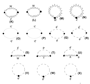
Figure 4: Vector and scalar boson contributions to the $W$ boson self energy. External $W$ lines are attached to the dots except those in (M), (N), (V), (W) and (X) to which two $W$ lines are attached.

$$\Sigma^{WW}(p) = \frac{i}{16\pi^{2}}\left[(-g^{2}c_{W}^{2})(\mbox{{\bf K}})+(-e^{2})(\mbox{{\bf L}})+\frac{1}{2}ig^{2}[2g_{\mu\nu}g_{\lambda\rho}-g_{\mu\lambda}g_{\nu\rho}-g_{\mu\rho}g_{\nu\lambda}](\mbox{{\bf M}})\right.$$

$$~{}~{}~{}~{}+\frac{1}{2}ig^{2}c_{W}^{2}(\mbox{{\bf N}})+(-2g^{2}c_{W}^{2})(\mbox{{\bf O}})+(-2e^{2})(\mbox{{\bf P}})+(-\frac{g^{2}}{4})(\mbox{{\bf Q}})$$

$$~{}~{}~{}~{}+(-\frac{g^{2}}{4})(\mbox{{\bf R}})+(-g^{2}M_{W}^{2})(\mbox{{\bf S}})+(-g^{2}M_{Z}^{2}s_{W}^{4})(\mbox{{\bf T}})+(-e^{2}M_{W}^{2})(\mbox{{\bf U}})$$

$$~{}~{}~{}~{}\left.+(\frac{ig^{2}}{4})(\mbox{{\bf V}})+(\frac{ig^{2}}{4})(\mbox{{\bf W}})+(\frac{ig^{2}}{2})(\mbox{{\bf X}})\right]$$

$$\Sigma^{WW}(0) = \frac{\alpha}{4\pi s_{W}^{2}}M_{W}^{2}\left[\left(\frac{s_{W}^{2}}{c_{W}^{2}}-1\right)\Delta_{W}+\frac{3}{4(1-c_{W}^{2}/h)}\ln\frac{c_{W}^{2}}{h}-\frac{h}{8c_{W}^{2}}\right.$$ (5.116)

$$+\left.\left(s_{W}^{2}+\frac{s_{W}^{4}}{c_{W}^{2}}-\frac{1}{8c_{W}^{2}}-\frac{39}{12}+\left(\frac{s_{W}^{2}}{c_{W}^{2}}+3-\frac{17}{4s_{W}^{2}}\right)\ln c_{W}^{2}\right)\right],$$

$$\Sigma^{WW}(M_{W}^{2}) = \frac{\alpha}{4\pi}\frac{1}{s_{W}^{2}}M_{W}^{2}\left[-\left(\frac{25}{6}-\frac{s_{W}^{2}}{c_{W}^{2}}\right)\Delta_{W}\right.$$ (5.117)

$$+\left(\frac{1}{12c_{W}^{4}}+\frac{4}{3c_{W}^{2}}-\frac{17}{3}-4c_{W}^{2}\right)(C(M_{W}^{2},M_{Z},M_{W})-\ln c_{W})$$

$$\left(1-\frac{h}{3c_{W}^{2}}+\frac{1}{12}\frac{h^{2}}{c_{W}^{4}}\right)\left(C(M_{W}^{2},M_{H},M_{W})-\frac{1}{2}\ln\frac{c_{W}^{2}}{h}\right)$$

$$-\frac{h}{h-c_{W}^{2}}\ln\frac{h}{c_{W}^{2}}\left(\frac{7}{4}-\frac{h}{3c_{W}^{2}}+\frac{h^{2}}{12c_{W}^{4}}\right)$$

$$+\left[\frac{1}{12c_{W}^{4}}+\frac{7}{3c_{W}^{2}}-\frac{107}{12}-10c_{W}^{2}\right]\frac{1}{1-c_{W}^{2}}\ln c_{W}^{2}$$

$$\left.+\frac{1}{12c_{W}^{4}}+\frac{13}{6c_{W}^{2}}-\frac{233}{18}-\frac{h}{2c_{W}^{2}}+\frac{h^{2}}{12c_{W}^{4}}-4c_{W}^{2}\right].$$

5.5 Expressions of $\Delta\alpha,\Delta\rho$ and $\Delta r$

(1) $\Delta\alpha$
$\Delta\alpha$ is defined by the subtracted photon vacuum polarization and is composed of four contributions,

$$\Delta\alpha = -Re\Pi^{\gamma}(M_{Z}^{2})+\Pi^{\gamma}(0)$$ (5.118)

$$= \Delta\alpha_{lept}+\Delta\alpha_{had}^{(5)}+\Delta\alpha_{top}+\Delta\alpha_{W}.$$

The leptonic subtracted part, $\Delta\alpha_{lept}$, is given by

$$\Delta\alpha_{lept} = -Re\Pi^{\gamma}_{lept}(M_{Z}^{2})+\Pi^{\gamma}_{lept}(0)$$ (5.119)

$$= \sum_{l=e,\mu,\tau}\frac{\alpha}{3\pi}\left(\ln{\frac{M_{Z}^{2}}{m_{l}^{2}}}-\frac{5}{3}\right).$$

We note that the 5 flavor contributions to $\Delta\alpha^{(5)}_{had}=0.02804(65)$ can be derived from experimental data with the help of a dispersion relation^[17]

$$\Delta\alpha^{(5)}_{had}=Re\left(-\frac{\alpha}{3\pi}M_{Z}^{2}\right.\int^{\infty}_{4m_{\pi}^{2}}ds^{\prime}\left.\frac{R^{\gamma}(s^{\prime})}{s^{\prime}(s^{\prime}-M_{Z}^{2}-i\epsilon)}\right),$$ (5.120)

with

$$R^{\gamma}(s)=\frac{\sigma(e^{+}e^{-}\rightarrow\gamma^{*}\rightarrow hadrons)}{\sigma(e^{+}e^{-}\rightarrow\gamma^{*}\rightarrow\mu^{+}\mu^{-})},$$ (5.121)

as an experimental quantity up to a scale $s_{1}$ and applying perturbative QCD for the tail region above $s_{1}$. The contribution of a heavy top quark is

$$\Delta\alpha_{top}\simeq-\frac{\alpha}{\pi}Q_{t}^{2}\frac{M_{Z}^{2}}{5m_{t}^{2}}$$ (5.122)

It can be seen that $W$ boson contribution to $\Delta\alpha$ can be evaluated by using eq.(5.97),

$$\Delta\alpha_{W}=\frac{\alpha}{4\pi}\left[(3+4c_{W}^{2})C(M_{Z}^{2},M_{W},M_{W})-\frac{2}{3}\right],$$ (5.123)

which is negligible. Then, we may take $\Delta\alpha$ as,

$$\Delta\alpha = \frac{\alpha}{3\pi}\sum_{l}Q_{l}^{2}\left(\ln{\frac{M_{Z}^{2}}{m_{l}^{2}}}-\frac{5}{3}\right)+\Delta\alpha^{(5)}_{had}$$ (5.124)

$$= 0.05940(65).$$

(2) $\Delta\rho$
The fermionic contribution to $\Delta\rho$ is calculated from the formulae

$$\Delta\rho=\frac{\Sigma^{ZZ}(0)}{M^{2}_{Z}}-\frac{\Sigma^{WW}(0)}{M^{2}_{W}}.$$ (5.125)

For a doublet of fermions with masses $(m_{1},m_{2})$, it is in general given by

$$(\Delta\rho)_{ferm}=N_{c}\frac{\alpha}{16\pi s_{W}^{2}c_{W}^{2}M_{Z}^{2}}\left(m_{1}^{2}+m_{2}^{2}-\frac{2m_{1}^{2}m_{2}^{2}}{m_{1}^{2}-m_{2}^{2}}\right.\left.\ln\frac{m_{1}^{2}}{m_{2}^{2}}\right).$$ (5.126)

We can see that their singular parts cancel and that the contributions of the quarks except top quark are very small. Then a finite term which is quadratic in $m_{t}$ remains

$$(\Delta\rho)_{ferm}=\frac{3\alpha}{16\pi s_{W}^{2}c_{W}^{2}}\frac{m_{t}^{2}}{M_{Z}^{2}}.$$ (5.127)

The Higgs mass dependence in $\Delta\rho$, up to one-loop order, is given by

$$(\Delta\rho)_{H} = \frac{3\alpha}{16\pi s_{W}^{2}}\left\{\frac{1}{c_{W}^{2}}\left(\Delta-\ln\frac{M_{Z}^{2}}{\mu^{2}}\right)-\left(\Delta-\ln\frac{W_{Z}^{2}}{\mu^{2}}\right)+\frac{5}{6}\frac{s_{W}^{2}}{c_{W}^{2}}\right.$$ (5.128)

$$~{}~{}~{}~{}~{}\left.+\frac{h}{c_{W}^{2}(1-h)}\ln h-\frac{h}{c_{W}^{2}-h}\ln{\frac{h}{c_{W}^{2}}}\right\}.$$

(3) $\Delta r$
To the one-loop order, the contributions to the $\mu-$ decay amplitude are obtained by adding the diagrams,

Figure 5: $\mu-$ decay amplitude

The vertex corrections and box diagrams in the $\mu-$ decay amplitude are shown in Fig.5.

Figure 6: vertex and box contributions

Then, using the bare parameter relations (5.13-5.15), $G_{\mu}/\sqrt{2}$ can be written as

$$\frac{G_{\mu}}{\sqrt{2}} = \frac{e^{2}_{0}}{8s_{W}^{02}M_{W}^{02}}\left[1+\frac{\Sigma^{WW}(0)}{M_{W}^{2}}+[\mbox{{\bf vertex}}]+[\mbox{{\bf box}}]\right]$$ (5.129)

$$= \frac{e^{2}}{8s_{W}^{2}M_{W}^{2}}\left[1+2\frac{\delta e}{e}-\frac{c_{W}^{2}}{s_{W}^{2}}\right.\left(\frac{\delta M_{Z}^{2}}{M_{Z}^{2}}\right.-\left.\frac{\delta M_{W}^{2}}{M_{W}^{2}}\right)-\frac{\delta M_{W}^{2}}{M_{W}^{2}}\left.+\frac{\Sigma^{WW}(0)}{M_{W}^{2}}+[\mbox{{\bf vertex}}]+[\mbox{{\bf box}}]\right]$$

$$\equiv \frac{\pi\alpha}{2s_{W}^{2}M_{W}^{2}}[1+\Delta r],$$

where we have used the relations $e_{0}^{2}=e^{2}\left(1+2\frac{\delta e}{e}\right)$, $M_{W}^{02}=M_{W}^{2}+\delta M_{W}^{2}$ and

$$\sin^{2}\theta_{W}^{0}=\sin^{2}\theta_{W}+\cos^{2}\theta_{W}\left(\frac{\delta M_{Z}^{2}}{M_{Z}^{2}}\right.-\left.\frac{\delta M_{W}^{2}}{M_{W}^{2}}\right),$$ (5.130)

and

$$[\mbox{{\bf vertex}}]+[\mbox{{\bf box}}] = \frac{\alpha}{\pi s_{W}^{2}}\Delta_{W}+\frac{\alpha}{4\pi s_{W}^{2}}\left(6+\frac{7-4s_{W}^{2}}{2s_{W}^{2}}\ln{c_{W}^{2}}\right)$$ (5.131)

$$= \frac{2}{c_{W}s_{W}}\frac{\Sigma^{\gamma Z}(0)}{M_{Z}^{2}}+\frac{\alpha}{4\pi s_{W}^{2}}\left(6+\frac{7-4s_{W}^{2}}{2s_{W}^{2}}\ln{c_{W}^{2}}\right),$$

where we have used the result eq.(5.98). Then,

$$\Delta r = \Pi^{\gamma}(0)-\frac{c_{W}^{2}}{s_{W}^{2}}\left(\frac{\delta M_{Z}^{2}}{M_{Z}^{2}}\right.-\left.\frac{\delta M_{W}^{2}}{M_{W}^{2}}\right)-\frac{\delta M_{W}^{2}-\Sigma^{WW}(0)}{M_{W}^{2}}$$ (5.132)

$$+2\frac{c_{W}^{2}}{s_{W}^{2}}\frac{\Sigma^{\gamma Z}(0)}{M_{Z}^{2}}+\frac{\alpha}{4\pi s_{W}^{2}}\left(6+\frac{7-4s_{W}^{2}}{2s_{W}^{2}}\ln{c_{W}^{2}}\right)$$

$$= \Pi^{\gamma}(0)-Re\Pi^{\gamma}(M_{Z}^{2})-\frac{c_{W}^{2}}{s_{W}^{2}}\left(\frac{\Sigma^{ZZ}(0)}{M_{Z}^{2}}\right.-\left.\frac{\Sigma^{WW}(0)}{M_{W}^{2}}\right)$$

$$+Re\Pi^{\gamma}(M_{Z}^{2})+2\frac{c_{W}}{s_{W}}\frac{\Sigma^{\gamma Z}(0)}{M_{Z}^{2}}-\frac{Re\Sigma^{WW}(M_{W}^{2})-\Sigma^{WW}(0)}{M_{W}^{2}}+$$

$$-\frac{c_{W}^{2}}{s_{W}^{2}}\left[\frac{Re\Sigma^{ZZ}(M_{Z}^{2})-\Sigma^{ZZ}(0)}{M_{Z}^{2}}\right.-\left.\frac{Re\Sigma^{WW}(M_{W}^{2})-\Sigma^{WW}(0)}{M_{W}^{2}}\right]+\cdots$$

$$= \Delta\alpha-\frac{c_{W}^{2}}{s_{W}^{2}}\Delta\rho+(\Delta r)_{rem}.$$

It should be noted that the remainder term also contains a logarithmic term in the top mass,

$$(\Delta r)^{top}_{rem}=\frac{\alpha}{4\pi s_{W}^{2}}\left(\frac{c_{W}^{2}}{s_{W}^{2}}-\frac{1}{3}\right)\ln{\frac{m_{t}}{M_{Z}}}.$$ (5.133)

Also the Higgs boson contribution is part of the remainder and is given by

$$(\Delta r)^{Higgs}_{rem} = \frac{\alpha}{4\pi s^{4}_{W}}\left\{\left(\frac{h}{3}-1-\frac{h^{2}}{12}\right)\right.\left(C(M_{Z}^{2},M_{H},M_{Z})-1+\frac{h+1}{2(h-1)}\ln h\right)$$ (5.134)

$$+\left(2-\frac{1}{c_{W}^{2}}\right)\left(c_{W}^{2}-\frac{h}{3}+\frac{h^{2}}{12c_{W}^{2}}\right)\left(C(M_{W}^{2},M_{H},M_{W})-1+\frac{h+c_{W}^{2}}{2(h-c_{W}^{2})}\ln\frac{h}{c_{W}^{2}}\right)$$

$$+\left(\frac{11}{24}-\frac{h}{12}\right)\frac{h+1}{h-1}\ln h+\left(\frac{11}{24}+\frac{h}{12}-\frac{3}{4}\frac{c_{W}^{2}h}{h-c_{W}^{2}}\right)\ln\frac{h}{c_{W}^{2}}$$

$$\left.-\left(\frac{3}{8}-\frac{h}{12}\right)\ln c_{W}^{2}+s_{W}^{2}\left(\frac{1}{24}\frac{h}{c_{W}^{2}}-\frac{59}{72}\right)\right\},$$

where we choose the renormalization scale as $\mu^{2}=M_{Z}^{2}$. For large $M_{H}$, it increases only logarithmically,

$$(\Delta r)^{Higgs}_{rem}\simeq\frac{\alpha}{16\pi s_{W}^{2}}\frac{11}{3}\left(\ln{\frac{M_{H}^{2}}{M_{W}^{2}}}-\frac{5}{6}\right).$$ (5.135)

The explicit form of $\Delta r$ is written as

$$\Delta r = (\Delta r)_{ferm}+(\Delta r)_{boson},$$ (5.136)

$$(\Delta r)_{ferm} = (\Delta\alpha)_{ferm}-\frac{\alpha}{4\pi s_{W}^{4}}\left[\left(\frac{1}{2}-\frac{2}{3}s_{W}^{2}\right)\ln\frac{M_{Z}^{2}}{m_{t}^{2}}-\left(\frac{5}{6}-\frac{10}{9}s_{W}^{2}+\frac{20}{27}s_{W}^{4}\right)\right.$$ (5.137)

$$\left.+\left(\frac{16}{45}s_{W}^{4}+\frac{4}{3}s_{W}^{2}-\frac{19}{40}\right)\frac{M_{Z}^{2}}{m_{t}^{2}}\right]+\sum_{f\neq t}\frac{\alpha}{4\pi s_{W}^{2}}\left(1-\frac{c_{W}^{2}}{s_{W}^{2}}\right)\frac{N_{c}^{f}}{6}\ln c_{W}^{2}+\cdots,$$

$$(\Delta r)_{boson} = (\Delta\alpha)_{W}+\frac{\alpha}{4\pi s_{W}^{4}}\left\{\left(s-\frac{1}{c_{W}^{2}}\right)\left(\frac{1}{12c_{W}^{2}}+\frac{4}{3}-\frac{17}{3}c_{W}^{2}-4c_{W}^{4}\right)C(M_{W}^{2},M_{Z},M_{W})\right.$$ (5.138)

$$+\left(\frac{32}{3}c_{W}^{4}+\frac{2}{3}c_{W}^{2}-\frac{37}{12}\right)C(M_{Z}^{2},M_{W},M_{W})+\left(\frac{1}{3}h-1-\frac{h^{2}}{12}\right)C(M_{Z}^{2},M_{H},M_{Z})$$

$$+\left(2-\frac{1}{c_{W}^{2}}\right)\left(c_{W}^{2}-\frac{1}{3}h+\frac{h^{2}}{12c_{W}^{2}}\right)C(M_{W}^{2},M_{H},M_{W})$$

$$+\ln\frac{h}{c_{W}^{2}}(c_{W}^{2}-s_{W}^{2})\left[\frac{1}{2}-\frac{1}{6c_{W}^{2}}+\frac{h^{2}}{24c_{W}^{4}}-\frac{h}{h-c_{W}^{2}}\left(\frac{7}{4}-\frac{h}{3c_{W}^{2}}+\frac{h^{2}}{12c_{W}^{4}}-\frac{3}{4}\frac{s_{W}^{2}}{c_{W}^{2}-s_{W}^{2}}\right)\right]$$

$$+\left(\frac{1}{2}-\frac{h}{12}-\frac{h^{2}}{24}\right)\ln h+\left(\frac{11}{6}-\frac{3}{4c_{W}^{2}}-\frac{141}{6}c_{W}^{2}-24c_{W}^{4}+\frac{1}{12s_{W}^{4}}-\frac{1}{6s_{W}^{2}}\right)\ln c_{W}^{2}$$

$$+\frac{h}{24}\left(2h+\frac{9}{c_{W}^{2}}-13+\frac{4h}{c_{W}^{2}}-\frac{2h}{c_{W}^{4}}\right)+\frac{211}{24}+\frac{23}{8c_{W}^{2}}+\frac{13}{12c_{W}^{4}}-\frac{233}{12}c_{W}^{2}$$

$$\left.+6s_{W}^{2}+\frac{7-4s_{W}^{2}}{2}\ln c_{W}^{2}\right\}.$$

5.6 Higher order corrections

There are large logarithms of the form $\alpha^{n}\ln^{m}(M_{Z}^{2}/m_{f}^{2})$ in the context of the effective electromagnetic charge. These corrections are effectively incorporated when the one-loop correction $1+\Delta\alpha$ is replaced by $\frac{1}{1-\Delta\alpha}$ according to renormalization group arguments^[18].

Due to large mass of top quark, the next-leading large contributions to $\Delta\rho$ have to be considered, which are $O(G_{\mu}^{2}m_{t}^{4})^{[19]},O(\alpha_{s}G_{\mu}m_{t}^{2})^{[20,21]}$ and $O(\alpha_{s}^{2}G_{\mu}m_{t}^{2})^{[22]}$. Including the first two corrections, we can write the parameter $\Delta\rho$ as

$$\Delta\rho=3x_{t}\left[1+x_{t}\rho^{(2)}(\frac{M_{H}}{m_{t}})\right.\left.-2\alpha_{s}(m_{t})\frac{\pi^{2}+3}{9\pi}\right].$$ (5.139)

where $x_{t}=G_{\mu}m_{t}^{2}/8\pi^{2}\sqrt{2}$ and $\rho^{(2)}$ is strongly dependent on $M_{H}^{[19]}$. For light Higgs boson $M_{H}<<m_{t}$, the function $\rho^{(2)}$ is $19-2\pi^{2}$ and for heavy Higgs $M_{H}>>m_{t}$, it is given by the asymptotic expression with $r=M_{H}/m_{t}$,

$$\rho^{(2)}=6\ln^{2}r-27\ln r+\frac{49}{4}\pi^{2}+O(\ln^{2}r/r^{2})$$ (5.140)

The third term is originated from $t\bar{t}$ threshold, which is discussed elsewhere^[19]. Though the QCD corrections in $\Delta\rho$ are sufficient for very large top mass $m_{t}>>M_{W}$, one can take into account the subleading corrections $O(\alpha_{s}G_{\mu}M_{W}^{2})^{[19]}$ for realistic values of $m_{t}$. They can amount to 20 % of the perturbative QCD correction to $\Delta r$ at $m_{t}=150~{}\mbox{GeV}$. We will include above corrections except $t\bar{t}$ threshold in the ZFITTER, as well as the dominant two-loop corrections^[19] of $O(\alpha^{2}m_{t}^{2})$ to $\Delta\rho=1-1/\rho$ and the QCD corrections to the leading electroweak one-loop term^[23] of $O(\alpha\alpha_{s}m_{t}^{2})$ and $O(\alpha\alpha_{s}^{2}m_{t}^{2})$. These new theoretical advances in radiative corrections coupled with the experimental developments in the electroweak data, $m_{t}$ and $M_{W}$ are additional reasons to update the precision tests of the SM.

Thanks to the higher order corrections in $\Delta\alpha$ and $\Delta\rho$, Eq. (5.116) can be written as

$$\sqrt{2}G_{\mu}=\frac{\pi\alpha}{M_{W}^{2}\sin^{2}\theta_{W}}\left[\frac{1}{(1-\Delta\alpha)\cdot(1+\frac{\cos^{2}\theta_{W}}{\sin^{2}\theta_{W}}\Delta\rho)}+\Delta r_{remainder}\right].$$ (5.141)

The proper incorporation of the non-leading high order terms containing mass singularities of the type $\alpha^{2}\ln(M_{Z}/m_{f})$ enable us to rewrite eq.(5.128) as

$$\sqrt{2}G_{\mu} = \frac{\pi\alpha}{M_{W}^{2}\sin^{2}\theta_{W}}\left[~{}\frac{1}{(1-\Delta\alpha)\cdot(1+\frac{\cos^{2}\theta_{W}}{\sin^{2}\theta_{W}}\Delta\rho)-\Delta r_{remainder}}~{}\right]$$ (5.142)

$$\equiv \frac{\pi\alpha}{M_{W}^{2}\sin^{2}\theta_{W}}\frac{1}{1-\Delta r}.$$

5.7 $Z$ physics in $e^{+}e^{-}\rightarrow f\bar{f}$

Following the general principles discussed above we attach multiplicative renormalization constants to each free parameter and each symmetry multiplet of fields in the symmetric Lagrangian:

$$W_{\mu}^{a} \rightarrow (Z_{2}^{W})^{1/2}W_{\mu}^{a}$$

$$B_{\mu} \rightarrow (Z_{2}^{B})^{1/2}B_{\mu}$$

$$\psi^{L}_{j} \rightarrow (Z^{j}_{L})^{1/2}\psi^{L}_{j}$$

$$\psi^{R}_{j\sigma} \rightarrow (Z^{j\sigma}_{R})^{1/2}\psi^{R}_{j\sigma}$$

$$\Phi \rightarrow (Z^{\Phi})^{1/2}\Phi$$

$$g_{2} \rightarrow Z_{1}^{W}(Z_{2}^{W})^{-3/2}g_{2}$$

$$g_{1} \rightarrow Z_{1}^{B}(Z_{2}^{B})^{-3/2}g_{1}$$

$$v \rightarrow (Z^{\Phi})^{1/2}(v-\delta v)$$

$$g_{j\sigma} \rightarrow (Z^{\Phi})^{-1/2}Z_{1}^{j\sigma}g_{j\sigma}$$

$$\mu^{2} \rightarrow (Z^{\Phi})^{-1}(\mu^{2}-\delta\mu^{2})$$

$$\lambda \rightarrow (Z^{\Phi})^{-2}Z_{\lambda}\lambda$$ (5.143)

where the RHS represent the bare fields and parameters, the quantities without the $Z$-factors are the corresponding renormalized fields and parameteres and the variation of the renormalization constants is given by $Z_{i}=1+\delta Z_{i}$, and

$$\left(\begin{array}[]{c}\delta Z_{i}^{\gamma}\\ \delta Z_{i}^{Z}\end{array}\right)=\left(\begin{array}[]{cc}s_{W}^{2}&c_{W}^{2}\\ c_{W}^{2}&s_{W}^{2}\end{array}\right)\left(\begin{array}[]{c}\delta Z_{i}^{W}\\ \delta Z_{i}^{B}.\end{array}\right).$$ (5.144)

Field renormalization ensures that we end up with finite Green functions. The field renormalization in (5.130) is performed in a way that it respects the gauge symmetry by introducing the minimal number of field renormalization constants. Therefore also the counter term Lagrangian and the renormalized Green functions reflect the gauge symmetry. The price for this, however, is that not all residues of the propagators can be normalized to unity. As a consequence, any calculation with the renormalized Lagrangian will have to include finite multiplicative wave function renormalization factors for some of the external lines in S matrix elements.

It is of course possible to perform the renormalization in such a way that these finite corrections do not appear^{[24,25,26,26]}. But then the Lagrangian will contain many constants which have to be calculated in terms of the few fundamental parameters.

The independent renormalization of the Higgs vacuum expectation value $v$ absorbs the linear term in the Higgs potential, which is induced by the appearance of tadpole diagrams in one-loop order, in such a way that the relation $v=\frac{2\mu}{\sqrt{\lambda}}$ remains valid for the renormalized parameters with $v$ being the minimum of the Higgs potential at the one-loop level. As a practical consequence of this tadpole renormalization, all tadpole graphs can be omitted in the renormalized amplitudes and Green functions. They are, however, necessary to make the mass counter terms gauge independent.

The systematic way for obtaining results for physical amplitudes in one-loop order is scheduled as follows: The expansion (5.16) yields the renormalized Lagrangian $\cal{L}$ which can now be re-parametrized in terms of the physical parameters $e,M_{W},M_{Z},M_{H},m_{f}$ and the physical fields $A_{\mu},Z_{mu},W_{\mu}^{\pm},H$ (also the unphysical Higgs field components $\phi^{\pm},\eta$ and the ghost fields $\eta_{\pm},\eta_{0},\eta_{A}$ are present in the $R_{\xi}$ gauge), and the counter term Lagrangian $\delta\cal{L}$. From $\delta\cal{L}$ the counter term Feynman rules are derived. After rewriting them in terms of $e,M_{W},M_{Z},M_{H},m_{f}$ the counter term graphs have to be added to the 1-loop vertex functions calculated from $\cal{L}$. The renormalization constants in (5.16) are fixed afterwards by imposing the appropriate renormalization conditions. The results are finite Green functions in terms of the above physical parameter set from which the S matrix elements for all processes of interest can be obtained. Then the renormalized gauge boson self energies ($\tilde{\Sigma}$) can be expressed in terms of the non-renormalized ones ($\Sigma$),

$$\tilde{\Sigma}^{\gamma\gamma}(k^{2}) = \Sigma^{\gamma\gamma}(k^{2})-k^{2}\Pi^{\gamma}(0)$$ (5.145)

$$\tilde{\Sigma}^{\gamma Z}(k^{2}) = \Sigma^{\gamma Z}(k^{2})-\Sigma^{\gamma Z}(0)+k^{2}\left[2\frac{\Sigma^{\gamma Z}(0)}{M_{Z}^{2}}\right.-\frac{c_{W}}{s_{W}}\left(\frac{\delta M_{Z}^{2}}{M_{Z}^{2}}\right.-\left.\left.\frac{\delta M_{W}^{2}}{M_{W}^{2}}\right)\right]$$ (5.146)

$$\tilde{\Sigma}^{ZZ}(k^{2}) = \Sigma^{ZZ}(k^{2})-\delta M_{Z}^{2}+\delta Z_{2}^{Z}(k^{2}-M_{Z}^{2})$$ (5.147)

$$\tilde{\Sigma}^{WW}(k^{2}) = \Sigma^{WW}(k^{2})-\delta M_{W}^{2}+\delta Z_{2}^{W}(k^{2}-M_{W}^{2})$$ (5.148)

with

$$\delta Z_{2}^{Z} = -\Pi^{\gamma}(0)-2\frac{c_{W}^{2}-s_{W}^{2}}{s_{W}c_{W}}\frac{\Sigma^{\gamma Z}(0)}{M_{Z}^{2}}+\frac{c_{W}^{2}-s_{W}^{2}}{s_{W}^{2}}\left(\frac{\delta M_{Z}^{2}}{M_{Z}^{2}}\right.-\left.\frac{\delta M_{W}^{2}}{M_{W}^{2}}\right)$$ (5.149)

$$\delta Z_{2}^{W} = -\Pi^{\gamma}(0)-2\frac{c_{W}}{s_{W}}\frac{\Sigma^{\gamma Z}(0)}{M_{Z}^{2}}+\frac{c_{W}^{2}}{s_{W}^{2}}\left(\frac{\delta M_{Z}^{2}}{M_{Z}^{2}}\right.-\left.\frac{\delta M_{W}^{2}}{M_{W}^{2}}\right)$$ (5.150)

Replacing those renormalized self energies and renormalized masses with non-renormalized ones in eq.(5.25-5.27), one can obtain the renormalized gauge boson propagators. The two constant $Z_{W}$ and $Z_{B}$ are sufficient to make the self energies (resp. the propagators) and the vertex corrections finite. These additional two field renormalization constants allow to fullfil the further two renormalization conditions: vanishing of the $\gamma Z$ mixing propagator for real photons $(k^{2}=0)$; residue$=1$ for the photon propagator (in analogy to pure QED). The residues of the $W$ and $Z$ propagators, however, are different from unity.

(1) Effective neutral current couplings
The weak dressed $Z$ exchange amplitude can be written as follows

Figure 7: The $Z-$exchange amplitude and effective neutral current couplings

$$[\mbox{{\bf diagram~{} K}}] = \frac{e^{2}}{4s_{W}^{2}c_{W}^{2}}J^{(e)}\cdot\tilde{D}_{Z}(k^{2})\cdot J^{(f)}$$ (5.151)

$$= \frac{e^{2}}{4s_{W}^{2}c_{W}^{2}}\frac{J^{(e)}\cdot J^{(f)}}{[k^{2}-M_{Z}^{2}+\Sigma^{ZZ}(k^{2})]}$$

$$= \frac{e^{2}}{4s_{W}^{2}c_{W}^{2}}\frac{1}{[1+\Pi^{Z}(k^{2})]}\frac{J^{(e)}\cdot J^{(f)}}{[k^{2}-M_{Z}^{2}+iIm\Sigma^{ZZ}(k^{2})/[1+\Pi^{Z}(k^{2})]]}$$

where,

$$\Sigma^{ZZ}(k^{2}) = \tilde{\Sigma}^{ZZ}(k^{2})-\frac{\tilde{\Sigma}^{\gamma Z}(k^{2})}{k^{2}+\hat{\Sigma}^{\gamma\gamma}(k^{2})},$$ (5.152)

$$J^{(e)} = \bar{v}_{e}[\gamma_{\mu}(I_{3L}^{e}-2Q_{e}s_{W}^{2})-\gamma_{\mu}\gamma_{5}I_{3L}^{e}]u_{e},$$ (5.153)

$$J^{(f)} = \bar{u}_{f}[\gamma_{\mu}(I_{3L}^{f}-2Q_{f}s_{W}^{2})-\gamma_{\mu}\gamma_{5}I_{3L}^{f}]v_{f},$$ (5.154)

$$\Pi^{Z}(k^{2}) = \frac{Re\Sigma^{ZZ}(k^{2})-\delta M_{Z}^{2}}{k^{2}-M_{Z}^{2}}-\Pi^{\gamma}(0)+\frac{c_{W}^{2}-s_{W}^{2}}{s_{W}^{2}}\left(\frac{\delta M_{Z}^{2}}{M_{Z}^{2}}\right.-\frac{\delta M_{W}^{2}}{M_{W}^{2}}-2\frac{s_{W}}{c_{W}}\left.\frac{\Sigma^{\gamma Z}(0)}{M_{Z}^{2}}\right),$$ (5.155)

$$Re\Sigma^{ZZ}(k^{2}) = (k^{2}-M_{Z}^{2})\Pi^{Z}(k^{2}).$$ (5.156)

Then we can interpret the real part in the denominator of eq.(5.138) as the modified effective neutral current couplings. From the relation (5.129), we can see that

$$\frac{\pi\alpha}{s_{W}^{2}c_{W}^{2}}\frac{1}{1+\Pi^{Z}} = \sqrt{2}G_{\mu}M_{Z}^{2}\frac{1-\Delta r}{1+\Pi^{Z}}$$ (5.157)

$$= \sqrt{2}G_{\mu}M_{Z}^{2}[1+\Delta\rho+\cdots]$$

$$= \sqrt{2}G_{\mu}M_{Z}^{2}\rho_{f}.$$

The form factor $\rho_{f}$ can be expressed in terms of the self energy and vertex contributions which explicitly depend on the type of the external fermions,

$$\rho_{f}=1+\Delta\rho_{se}+\Delta\rho_{f,vertex}.$$ (5.158)

Here the self energy contributions are given by

$$\Delta\rho_{se}=\Delta\rho+\Delta\rho_{se,rem},$$ (5.159)

where

$$\Delta\rho = \frac{\Sigma^{ZZ}(0)}{M_{Z}^{2}}-\frac{\Sigma^{WW}(0)}{M_{W}^{2}}-2\frac{\sin\theta_{W}}{\cos\theta_{W}}\frac{\Sigma^{\gamma Z}(0)}{M_{Z}^{2}},$$ (5.160)

$$\Delta\rho_{se,rem} = \frac{\Sigma^{ZZ}(M_{Z}^{2})}{M_{Z}^{2}}-\frac{\Sigma^{ZZ}(0)}{M_{Z}^{2}}-\left(\frac{d\Sigma^{ZZ}}{dk^{2}}\right)(M_{Z}^{2}).$$ (5.161)

For the vertex contributions we get

$$\Delta\rho_{f,vertex} = \frac{\alpha}{16\pi s^{2}_{W}}\left[2(3v_{f}^{2}+a_{f}^{2})\Lambda_{2}(k^{2},M_{Z})-4c^{2}_{W}(1-2(1-|Q_{f}|)s^{2}_{W})\Lambda_{2}(k^{2},M_{W})\right.$$ (5.162)

$$\left.+24c_{W}^{4}\Lambda_{3}(k^{2},M_{W})\right]-\Delta r_{vertex+box},$$

where $\Delta r_{vertex+box}$ is given by eq.(5.118) and

$$\Lambda_{2}(k^{2},M) = -\frac{7}{2}-2\frac{M^{2}}{k^{2}}-\left(2\frac{M^{2}}{k^{2}}+3\right)\ln\frac{M^{2}}{k^{2}}$$ (5.163)

$$+2\left(1+\frac{M^{2}}{k^{2}}\right)^{2}\left[\ln{\left(\frac{M^{2}}{k^{2}}\right)}\ln{\left(\frac{1+M^{2}/k^{2}}{M^{2}/k^{2}}\right)}+\int^{1}_{0}\frac{dt}{t}\ln{\left(1+\frac{k^{2}}{M^{2}}t\right)}\right],$$

$$\Lambda_{3}(k^{2},M) = \frac{5}{6}-\frac{2M^{2}}{3k^{2}}+\frac{2}{3}\left(2\frac{M^{2}}{k^{2}}+1\right)\sqrt{4\frac{M^{2}}{k^{2}}-1}\arctan{\left[\frac{1}{\sqrt{4\frac{M^{2}}{k^{2}}-1}}\right]}$$ (5.164)

$$-\frac{3}{8}\frac{M^{2}}{k^{2}}\left(\frac{M^{2}}{k^{2}}+2\right)\left(\arctan{\frac{1}{\sqrt{4\frac{M^{2}}{k^{2}}-1}}}\right)^{2}~{}~{}~{}~{}~{}(for~{}~{}~{}k^{2}<4M^{2}).$$

In particular, we note that for $f=b$ the vertex corrections have a strong dependence on $m_{t}$. On can find the additional terms resulting from the heavy top quarks up to two-loop order,

$$\Delta\rho^{add}_{b,vertex} = -\frac{\alpha}{8\pi s_{W}^{2}}\left[\frac{m_{t}^{2}}{2M_{W}^{2}}+\left(\frac{8}{3}+\frac{1}{6c_{W}^{2}}\right)\ln\frac{m_{t}^{2}}{M_{W}^{2}}\right.$$ (5.165)

$$+\left.\frac{\alpha}{64\pi s_{W}^{2}}\left(\frac{m_{t}^{2}}{M_{W}^{2}}\right)^{2}(\tau^{(2)}-1)-\frac{\alpha_{s}}{2\pi}\frac{\pi^{2}-3}{3}\right],$$

where $\tau^{(2)}$ is the two-loop coefficient which depends on Higgs mass and is asymptotically given by $\tau^{(2)}=9-\frac{\pi}{3}$ for small Higgs masses ($M_{H}<<m_{t}$) and $\tau^{(2)}=\frac{1}{144}[311+24\pi^{2}+282\ln r+90\ln^{2}r-4r]$ for $M_{H}>2m_{t}$ ($r=(m_{t}/M_{H})^{2})$. The explicit form of $\rho_{f}$ is written by

$$\rho_{f} = 1+\frac{3\alpha m_{t}^{2}}{16\pi s_{W}^{2}M_{W}^{2}}+\frac{\alpha}{\pi}(v_{t}^{2}+a_{t}^{2})\frac{M_{Z}^{2}}{30m_{t}^{2}}+O(\frac{m^{2}_{f=light}}{M_{W}^{2}})$$ (5.166)

$$+\frac{\alpha}{4\pi s_{W}^{2}}\left\{\frac{1}{12c_{W}^{2}}\left[\left(-80c_{W}^{6}+8(c_{W}^{2}-s_{W}^{2})^{2}c_{W}^{2}+12c_{W}^{2}\right)C(M_{Z}^{2},M_{W},M_{W})\right.\right.$$

$$+\left(40c_{W}^{4}(1+2c_{W}^{2})-(c_{W}^{2}-s_{W}^{2})^{2}(1+8c_{W}^{2})-12c_{W}^{2}\right){\tilde{C}}(M_{Z}^{2},M_{W},M_{W})$$

$$+(12-6h+2h^{2})C(M_{Z}^{2},M_{H},M_{Z})-(12-4h+h^{2}){\tilde{C}}(M_{Z}^{2},M_{H},M_{Z})$$

$$\left.+(2h-h^{2}-2)+\left(-6-h+\frac{h^{2}}{2}+\frac{(h+1)}{2(h-1)}\right)\ln h\right]$$

$$+\left(\frac{1}{24c_{W}^{2}}+\frac{3h}{4(h-c_{W}^{2})}\right)\ln\frac{h}{c_{W}^{2}}+\frac{h}{8c_{W}^{2}}+\left(\frac{1}{24c_{W}^{2}}-2+\frac{17}{4s_{W}^{2}}\right)\ln c_{W}^{2}$$

$$\left.-\left(s_{W}^{2}+\frac{s_{W}^{4}}{c_{W}^{2}}-\frac{1}{8c_{W}^{2}}-\frac{39}{12}\right)\right\}$$

Also, the appearance of the $\gamma Z$ mixing beyond the tree level may be viewed as a redefinition of the neutral current vector coupling constants $v_{f},a_{f}$. This can be seen from

$$[\mbox{{\bf diagram~{} L}}] = \gamma_{\mu}(v_{f}-a_{f}\gamma_{5})+\gamma_{\mu}Q_{f}\frac{\Pi^{\gamma Z}(k^{2})}{1+\Pi^{\gamma}(k^{2})}$$ (5.167)

$$= \gamma_{\mu}\left[\frac{I_{3}^{f}-2Q_{f}s_{W}^{2}}{2s_{W}c_{W}}+Q_{f}\right.\left.\frac{\Pi^{\gamma Z}(k^{2})}{1+\Pi^{\gamma}(k^{2})}\right]-\frac{I_{3}^{f}}{2s_{W}c_{W}}\gamma_{\mu}\gamma_{5}$$

$$= \frac{1}{2s_{W}c_{W}}\left\{\gamma_{\mu}\left[I_{3}^{f}-2Q_{f}\left(s_{W}^{2}-s_{W}c_{W}\frac{\Pi^{\gamma Z}(k^{2})}{1+\Pi^{\gamma}(k^{2})}\right)\right]-I_{3}^{f}\gamma_{\mu}\gamma_{5}\right\}$$

where $\Pi^{\gamma}(k^{2})=\tilde{\Sigma}^{\gamma\gamma}(k^{2})/k^{2}$ and $\Pi^{\gamma Z}(k^{2})=\tilde{\Sigma}^{\gamma Z}(k^{2})/k^{2}.$ The last line of eq.(5.154) allows a redefinition of an effective mixing angle $\bar{s}_{W}^{2}$ as

$$\sin^{2}{\theta_{W}^{eff}}\equiv\bar{s}_{W}^{2} = s_{W}^{2}-s_{W}c_{W}Re\frac{\Pi^{\gamma Z}(k^{2})}{1+\Pi^{\gamma\gamma}(k^{2})}$$ (5.168)

$$\equiv \kappa_{f}s_{W}^{2}$$

where $\kappa_{f}=1-\frac{c_{W}}{s_{W}}\frac{\Pi^{\gamma Z}(k^{2})}{1+\Pi^{\gamma}(k^{2})}$. Similarly to the form factor $\rho_{f}$ we can express $\kappa_{f}$ as

$$\kappa_{f}=1+\Delta\kappa_{se}+\Delta\kappa_{f,vertex},$$ (5.169)

where

$$\Delta\kappa_{se} = \frac{c_{W}^{2}}{s_{W}^{2}}\Delta\rho+\Delta\kappa_{se,rem}$$ (5.170)

$$= \frac{\cos^{2}\theta_{W}}{\sin^{2}\theta_{W}}\left[\frac{\Sigma^{ZZ}(M_{Z}^{2})}{M_{Z}^{2}}-\frac{\Sigma^{WW}(M_{W}^{2})}{M_{W}^{2}}-\frac{\sin\theta_{W}}{\cos\theta_{W}}\frac{\Sigma^{\gamma Z}(M_{Z}^{2})+\Sigma^{\gamma Z}(0)}{M_{Z}^{2}}\right].$$

The vertex contributions of the light quarks are given by

$$\Delta\kappa_{f,vertex} = \frac{\alpha}{16\pi s_{W}^{2}}\left\{(1-4|Q_{f}|s_{W}^{2})(1-2|Q_{F}|s_{W}^{2})\right.\Lambda_{2}(M_{Z}^{2},M_{Z})$$ (5.171)

$$-\frac{2}{s_{W}^{2}}(1-2(1-|Q_{f}|)s_{W}^{2})\Lambda_{2}(M_{Z}^{2},M_{W})+\left.12\frac{c_{W}^{2}}{s_{W}^{2}}\Lambda_{3}(M_{Z}^{2},M_{W})\right\}.$$

For b quark, there are additional terms,

$$\Delta\kappa^{add}_{b,vertex} = -\frac{1}{2}\Delta\rho^{add}_{b,vertex}+6\left(\frac{\alpha m_{t}}{8\pi M_{W}^{2}s^{2}_{W}}\right)^{2}.$$ (5.172)

The explicit form of $\kappa_{f}$ turns out to be

$$\kappa_{f} = 1-\frac{\alpha}{4\pi s_{W}^{4}}\left\{-\frac{1}{2}\frac{m_{t}^{2}}{M_{Z}^{2}}+\left(\frac{1}{6}-\frac{2}{3}c_{W}^{2}+\frac{11}{6}\frac{m_{t}^{2}}{M_{Z}^{2}}-\frac{4}{3}c_{W}^{2}\frac{m_{t}^{2}}{M_{Z}^{2}}\right)C(M_{Z}^{2},m_{t},m_{t})\right.$$ (5.173)

$$+\left(c_{W}^{2}-\frac{1}{2}\frac{m_{t}^{2}}{M_{Z}^{2}}-\frac{1}{2}\frac{m_{t}^{4}}{c_{W}^{2}M_{Z}^{4}}\right)C(M_{W}^{2},m_{t},0)+\left(\frac{1}{6}+\frac{1}{3}c_{W}^{2}\right)\ln\frac{M_{Z}^{2}}{m_{t}^{2}}$$

$$+\left(\frac{1}{12}+\frac{17}{6}c_{W}^{2}+\frac{16}{3}c_{W}^{4}\right)C(M_{Z}^{2},M_{W},M_{W})$$

$$+\left(\frac{1}{12c_{W}^{2}}+\frac{4}{3}-\frac{17}{3}c_{W}^{2}-4c_{W}^{4}\right)C(M_{W}^{2},M_{Z},M_{W})$$

$$+\left(-1+\frac{h}{3}-\frac{h^{2}}{12}\right)C(M_{Z}^{2},M_{H},M_{Z})+\left(c_{W}^{2}-\frac{h}{3}+\frac{h^{2}}{12c_{W}^{2}}\right)C(M_{W}^{2},M_{H},M_{W})$$

$$-\frac{h^{2}-1}{24}\ln h+\ln\frac{h}{c_{W}^{2}}\left[\left(\frac{11}{24}+\frac{h}{4}-\frac{c_{W}^{2}}{2}-\frac{h^{2}}{24c_{W}^{2}}\right)\right.$$

$$\left.+\frac{h}{h-c_{W}^{2}}\left(\frac{1}{4}c_{W}^{2}-\frac{h}{3}+\frac{h^{2}}{12c_{W}^{2}}\right)\right]-\ln c_{W}^{2}\left[-\frac{h}{12}+\frac{33}{4(1-c_{W}^{2})}-\frac{69}{8}-3c_{W}^{2}\right.$$

$$\left.\left.+\frac{1+c_{W}^{2}}{1-c_{W}^{2}}\left(\frac{1}{24c_{W}^{2}}+\frac{2}{3}-\frac{17}{6}c_{W}^{2}-2c_{W}^{4}\right)\right]-\frac{3}{4}-\frac{43}{6}c_{W}^{2}+8c_{W}^{4}-\frac{1}{12c_{W}^{2}}-\frac{h^{2}s_{W}^{2}}{12c_{W}^{2}}\right\}$$

(2) $Z$ decay width
With the help of the form factors, $\kappa_{f}$ and $\rho_{f}$, we can calculate the $Z$ width $\Gamma_{Z}$. It can be expressed as the sum over the fermionic partial decay widths

$$\Gamma_{Z}=\sum_{f}\Gamma(Z\rightarrow f\bar{f})$$ (5.174)

to a good approximation because other rare decay modes contribute to $\Gamma_{Z}$ less than $0.1\%$. In terms of the effective coupling constants $\bar{V}^{2}_{f}$ and $\bar{A}_{f}^{2}$,

$$\bar{V}_{f}^{2} = \sqrt{\rho_{f}}(I_{3L}^{f}-2Q_{f}\kappa_{f}\sin^{2}\theta_{W})$$ (5.175)

$$\bar{A}_{f}^{2} = \sqrt{\rho_{f}}I_{3L}^{f},$$ (5.176)

the partial widths, $\Gamma(Z\rightarrow f\bar{f})$, can be written as

$$\Gamma(Z\rightarrow f\bar{f})=N_{c}^{f}\frac{M_{Z}^{3}}{12\pi}\sqrt{2}G_{\mu}~{}[\bar{V}^{2}_{f}+\bar{A}_{f}^{2}]~{}R_{QED}R_{QCD}.$$ (5.177)

The additional photonic QED and the gluonic corrections to the hadronic final state, $R_{QED}$ and $R_{QCD}$, are given by

$$R_{QED} = 1+\frac{3Q_{f}\alpha}{4\pi}$$ (5.178)

$$R_{QCD} = N_{c}\left[1+\frac{\alpha_{s}(M_{Z}^{2})}{\pi}+1.409\left(\frac{\alpha_{s}(M_{Z}^{2})}{\pi}\right)^{2}-12.77\left(\frac{\alpha_{s}(M_{Z}^{2})}{\pi}\right)^{3}\right]$$ (5.179)

where $N_{c}=1$ for leptons while $N_{c}=3$ for quarks. Note that the $Z\rightarrow f\bar{f}$ widths contain a number of additional corrections such as fermion mass effects and further QCD corrections proportional to the running quark mass $m_{q}^{2}(M_{Z}^{2})$. These contributions are very small for light quarks except $b$ quark. For $b$ quark, the additional corrections^[28] are $\Delta R_{QCD}=c_{1}(m_{b}^{2})\frac{\alpha_{s}(M_{Z}^{2})}{\pi}+c_{2}(m_{b}^{2},m_{t}^{2})\left(\frac{\alpha_{s}(M_{Z}^{2})}{\pi}\right)^{2}+c_{3}(m_{b}^{2})\left(\frac{\alpha_{s}(M_{Z}^{2})}{\pi}\right)^{3}~{}~{}$.

6 Precision Test of the Standard Model

Recent LEP measurements have improved so precise that LEP’s sensitivity can even detect the passing of TGV train, while the long-awaited top quark has now been measured. Those experimental advances should enable us to examine some important questions concerning the higher order radiative corrections and the existence of the Higgs boson for which we do not have direct evidence. In this paper, we will report the results of our precision tests of the standard electroweak model including the radiative corrections developed in section 5 with the 1995 electroweak precision data^[29] and the experimental $m_{t}^{[5]}$ and $M_{W}$. We will see that the precision test is sensitive not only to the choice of the data set, i.e. how many data points, but also to accuracy of the data used. The experimental data sets are from the measurements at LEP, SLD and Fermilab. In particular, the parameters $R_{b}$, $R_{c}$ from LEP and $\sin^{2}\theta^{lept}_{eff}$ from SLD should carefully be treated since the measurements of those parameters deviate significantly from the SM predictions. We will see how sensitive the indirect bounds of the Higgs boson mass are to those parameters. The Higgs boson mass range depends on whether or not the top quark mass $m_{t}$ is treated as constrained by the experimental mass range. Also we will show the uncertainty of the electroweak quantities in the precision tests to the choice of and the uncertainties in the input data as well as in the parameters $\alpha_{s}(M_{Z})$, $\alpha(M_{Z})$ and $m_{t}$. The new CDF result combined with the new D0 (as of spring 1996) reduced the uncertainty in $m_{t}$ significantly, i.e., $m_{t}=176\pm 13$ GeV. Also the preliminary D0 measurement (as of spring 1996) of the W boson mass revises the world average value, i.e., $M_{W}=80.26\pm 0.16$ GeV. In the present work we use these values of $m_{t}$ and $M_{W}$ along with the QCD and QED couplings $\alpha_{s}(M_{Z})$ and $\alpha(M_{Z})$ at the $Z$ mass scale as given by $\alpha_{s}(M_{Z})=0.123\pm 0.006$ corresponding to the value deduced from the event-shape measurements at LEP^[30] and $\alpha^{-1}(M_{Z})=128.89\pm 0.09^{[17]}$.

The electroweak sector of the standard model (SM) contains, besides the masses of the fermions and the Higgs bosons, three independent parameters, $g,g^{\prime}$ and $v$ which are the $SU(2)_{L}$, $U(1)_{Y}$ couplings and the vacuum expectation value of neutral component of the Higgs field. One can instead choose $g,M_{W}$ and $M_{Z}$ to be the three independent parameters. On the other hand, there are three fundamental parameters measured with high precision, which poses as the obvious choice of the three experimental inputs; the hyperfine structure constant $\alpha=1/137.0359895(61)$, the Fermi coupling constant from the muon decay $G_{\mu}=1.16639(2)\times 10^{-5}~{}\mbox{GeV}^{-2}$ and the $Z$ boson mass $M_{Z}=91.1884(22)$ GeV. What enters in the electroweak observable quantities is however the effective QED coupling constant $\alpha(M_{Z})$ at the $M_{Z}$ scale, which is known only within $0.1\%$ due to the uncertainty mainly in the hadronic contribution to the running of QED coupling from low energy to the $M_{Z}$ scale. With the choice of $\alpha(M_{Z}),G_{\mu}$, and $M_{Z}$ as the fundamental three input parameters, one can predict $M_{W}$ and the on-shell weak mixing angle $\sin^{2}{\theta_{W}}$.

The $W$-mass relation from the charge-current Fermi coupling constant depends on the higher order radiative correction $\Delta r$ which depends on the masses of the fermions including $m_{t}$, of the Higgs boson $m_{H}$ and the gauge bosons $M_{W}$ and $M_{Z}$ along with $\alpha_{s}(M_{Z})$ and $\alpha(M_{Z})$. Thus the $W$-boson mass determination should have a self-consistency, i.e., the $M_{W}$ entering in calculating the radiative correction $\Delta r$ should be the same as the final output $M_{W}$ from the $W$-mass relation. It is obvious that the $W$-mass relation can result only a correlation between $M_{W}$ and $m_{t}$ for a given $m_{H}$ or $M_{W}$ vs $m_{H}$ for given $m_{t}$ at the moment.

What distinguishes our work^[31] from other works of the precision test is the imposition of the consistency of $M_{W}$ in the minimal $\chi^{2}$-fit to the electroweak data. The $Z$-decay parameters are numerically calculated for the self-consistent sets of ($m_{t},m_{H},M_{W}$) and the minimal $\chi^{2}$-fit solution is searched by fitting them to the experimentally observed values. We present the results^[31] of the fits to the 1995 LEP and SLD data^[29] obtained by using the ZFITTER program^[32] that includes the dominant two-loop corrections^[18] of $O(\alpha^{2}m_{t}^{2})$ to $\Delta\rho=1-1/\rho$ and the QCD corrections to the leading electroweak one-loop term^[22] of $O(\alpha\alpha_{s}m_{t}^{2})$ and $O(\alpha\alpha_{s}^{2}m_{t}^{2})$. These new theoretical advances in radiative corrections coupled with the experimental developments in the electroweak data, $m_{t}$ and $M_{W}$ are additional reasons to update the precision tests of the SM.

6.1 Global fits to the LEP and SLD data

In Table 3, we give various sets of $(m_{t},m_{H})$ that give the best $\chi^{2}$ fits to the 1995 data of the eleven observables measured at LEP when $m_{t}$ is restricted to the range $176\pm 13$ GeV. Each set of $(m_{t},m_{H})$ is correlated self-consistently to the $W$-boson mass given in the first row in each case, i.e., these masses along with given lighter fermion masses and $\alpha(M_{Z})$ and $\alpha_{s}(M_{Z})$ give the radiative correction factor $\Delta r$ which in turn reproduces the $M_{W}$ from the $W$-mass relation. The errors in the electroweak parameters due to the uncertainty in QED and QCD coupling constants at $M_{Z}$ scale are also given in the parenthesis.

Numerical results in Table 3 show in general a good agreement with the SM predictions except for $R_{b}=R(\Gamma_{b\bar{b}}/\Gamma_{had})$ and $R_{c}=R(\Gamma_{c\bar{c}}/\Gamma_{had})$, which are about $3.5\sigma$ and $2.3\sigma$ away from the SM predictions, and are the major contributors to the $\chi^{2}$-value in the fits to the 1995 LEP data. Note that the deficiency in the predicted $R_{b}$ and the excess in $R_{c}$ (compared to the measured values) tend to decrease and thus the $\chi^{2}$ gets improved as $m_{t}$ is decreased toward the lower limit of the measurements. It is obvious therefore that the absolute minimal $\chi^{2}$-fit solution of the global fit to the 1995 LEP data would be reached for $m_{t}$ well below the experimental value. In fact the global minimal fit to the 1995 LEP data occurs when $m_{t}=145$ GeV and $m_{H}=42$ GeV with $\chi^{2}/dof=19.0/11$, which is to be compared to $m_{t}=176\pm 13$ GeV and $m_{H}>66$ GeV from the LEP search. On the other hand, if we choose to ignore $R_{b}$ and $R_{c}$ from the input data to fit, the global minimal solution occurs for $m_{t}=161$ GeV and $m_{H}=106$ GeV with significantly improved $\chi^{2}/dof=2.99/9$ and predicts $R_{b}=0.2162$ and $R_{c}=0.1722$. A similar result,( $m_{t}=160$ GeV, $m_{H}=93$ GeV ), follows with $\chi^{2}/dof=8.84/10$ when only $R_{b}$ is ignored from the input data set, which means that the global minimal solution is sensitive to $R_{b}$ data and favors to ignore the $R_{b}$ data. As shown in Table 3, the uncertainty in the predicted $m_{H}$ due to $\Delta\alpha^{-1}(M_{Z})=0.09$ and $\Delta\alpha_{s}(M_{Z})=0.006$ is about 100 GeV each around $m_{t}=175$ GeV. There is however a clear evidence of the electroweak radiative corrections in each of the electroweak $Z$-parameters. The best fit solutions to the 1995 LEP data with and without $R_{b}$ give a stable output $M_{W}=80.331(24)$ GeV for $m_{t}=176\pm 13$ GeV. $M_{W}$ can be shifted by another 13 MeV and 4 MeV due to uncertainties in $\alpha^{-1}(M_{Z})$ and $\alpha_{s}(M_{Z})$.

If we set $\alpha_{s}(M_{Z})$ free, the global minimal fit solution occurs at $\alpha_{s}(M_{Z})=0.123$ with the values of ($m_{t},m_{H})$ given above irrespectively of $R_{b}$ and $R_{c}$ in the data set. However the global minimal fit solution is achieved at $\alpha_{s}(M_{Z})=0.122$, for the combined set of LEP and SLD data as given in Table 4, with $(m_{t}=153~{}\mbox{GeV},m_{H}=27~{}\mbox{GeV},\chi^{2}/dof=28.3/14)$ for all data and with ($m_{t}=159~{}\mbox{GeV},m_{H}=36~{}\mbox{GeV},\chi^{2}/dof=11.7/12)$ if $R_{b}$ and $R_{c}$ are excluded from the fit. More or less the same result as the latter follows if only $R_{b}$ is excluded, suggesting that the effect of $R_{b}$ and $R_{c}$ are not so influential compared to the case of LEP data alone. The two $\alpha_{s}(M_{Z})$ values are well within the input value $\alpha_{s}(M_{Z})=0.123(6)$ used in our calculations. In particular, we note that inclusion of the SLD data makes the output $m_{H}$ to shift to even lower value, i.e., to $m_{H}=36$ GeV from $m_{H}=106$ GeV in the case of the LEP+SLD data set excluding $R_{b}$ and $R_{c}$.

Of the three data from SLD, $\sin^{2}\theta_{eff}^{lept}$ or $A_{LR}^{0}$ deviates the most from the SM prediction^[6] and therefore influences the most the minimal $\chi^{2}$-fit solution. To see this, we searched for the minimal $\chi^{2}$-solutions with the data sets including all three SLD parameters and only $\sin^{2}\theta_{eff}^{lept}$ with or without excluding $R_{b}$ and/or $R_{c}$ and found that they give the same results, for instance, $m_{t}=158$ GeV and $m_{H}=30$ GeV in the case of the LEP+SLD data set with $R_{b}$ excluded and with either all three or one SLD parameter $\sin^{2}\theta_{eff}^{lept}$ included. The $\chi^{2}/dof$ is $11.8/12$ and $8.15/10$ respectively. Thus it seems that either the SLD $\sin^{2}\theta_{eff}^{lept}$, if supported by further measurements, implies new physics beyond the SM or is not supported by the global precision test. Note also that the inclusion of the SLD data predicts from the minimal $\chi^{2}$-fit solutions a stable $W$-boson mass, $M_{W}=80.377(23)$ GeV where the error is due to $\Delta m_{t}=\pm 13$ GeV around 176 GeV. This is to be compared to the world average value $M_{W}=80.26\pm 0.16$ GeV. As before, there can be another shift of $13$ MeV and 4 MeV in $M_{W}$ due to $\Delta\alpha^{-1}=0.09$ and $\Delta\alpha_{s}=0.006$ respectively.

	(Experiment)
$m_{t}$ (GeV)	$176\pm 13$	$189$	$176$	$163$
$m_{H}$ (GeV)	60 $\leq m_{H}\leq 1000$	$578^{(213)(256)}_{(158)(168)}$	$276^{(110)(122)}_{(85)(82)}$	$123^{(61)(59)}_{(56)(34)}$
$M_{W}$ (GeV)	$80.26\pm 0.16$	$80.355(13)(4)$	$80.332(13)(4)$	$80.307(13)(4)$
$\Gamma_{Z}$ (MeV)	$2496.3\pm 3.2$	$2497.2(7)(32)$	$2497.0(7)(32)$	$2496.5(7)(33)$
$\sigma_{h}^{P}(nb)$	$41.488\pm 0.078$	$41.462(2)(32)$	$41.452(2)(32)$	$41.443(1)(32)$
$R(\Gamma_{had}/\Gamma_{l\bar{l}})$	$20.788\pm 0.032$	$20.757(5)(40)$	$20.769(5)(40)$	$20.781(5)(40)$
$A^{0,l}_{FB}$	$0.0172\pm 0.0012$	$0.0156(5)$	$0.0156(4)$	$0.0156(5)$
$A_{\tau}$	$0.1418\pm 0.0075$	$0.1442(20)$	$0.1440(20)$	$0.1441(20)$
$A_{e}$	$0.1390\pm 0.0089$	$0.1442(20)$	$0.1440(20)$	$0.1441(20)$
$R(\Gamma_{b\bar{b}}/\Gamma_{had})$	$0.2219\pm 0.0017$	$0.2152$	$0.2157$	$0.2161$
$R(\Gamma_{c\bar{c}}/\Gamma_{had})$	$0.1543\pm 0.0074$	$0.1725$	$0.1723$	$0.1722$
$A^{0.b}_{FB}$	$0.0999\pm 0.0031$	$0.1010(14)$	$0.1009(14)$	$0.1011(14)$
$A^{0.c}_{FB}$	$0.0725\pm 0.0058$	$0.0721(11)$	$0.0720(11)$	$0.0721(11)$
$\sin^{2}\theta^{lept}_{eff}$	$0.2325\pm 0.0013$	$0.2319(2)$	$0.2319(3)$	$0.2319(3)$
$\chi^{2}$		25.3	22.6	20.5

Table 3: Numerical results including full EWRC for eleven experimental parameters (the second column) of the Z-decay and $M_{W}$. Each pair of $m_{t}$ and $m_{H}$ represents the case of the best $\chi^{2}$- fit to the 1995 LEP data and $M_{W}=80.26(16)$ GeV for $\alpha_{s}(M_{Z})=0.123(6)$ and $\alpha^{-1}(M_{Z})=128.89(9)$. The numbers in the first and second () represent the explicit errors due to $\Delta\alpha^{-1}(M_{Z})=\pm 0.09$ and $\Delta\alpha_{s}(M_{Z})=\pm 0.006$ respectively.

	(Experiment)
$m_{t}$ (GeV)	$176\pm 13$	$189$	$176$	$163$
$m_{H}$ (GeV)	60 $\leq m_{H}\leq 1000$	$338^{(142)(102)}_{(106)(77)}$	$143^{(77)(48)}_{(57)(33)}$	$51^{(39)(12)}_{(24)(5)}$
$M_{W}$ (GeV)	$80.26\pm 0.16$	$80.400(13)(4)$	$80.379(13)(4)$	$80.354(13)(4)$
$\Gamma_{Z}$ (MeV)	$2496.3\pm 3.2$	$2499.4(7)(32)$	$2499.2(7)(32)$	$2497.8(7)(32)$
$\sigma_{h}^{P}(nb)$	$41.488\pm 0.078$	$41.460(1)(32)$	$41.451(1)(32)$	$41.441(1)(32)$
$R(\Gamma_{had}/\Gamma_{l\bar{l}})$	$20.788\pm 0.032$	$20.762(4)(40)$	$20.775(4)(40)$	$20.788(5)(40)$
$A^{0,l}_{FB}$	$0.0172\pm 0.0012$	$0.0161(4)$	$0.0162(4)$	$0.0163(5)$
$A_{\tau}$	$0.1418\pm 0.0075$	$0.1466(19)$	$0.1469(20)$	$0.1476(20)$
$A_{e}$	$0.1390\pm 0.0089$	$0.1466(19)$	$0.1469(20)$	$0.1476(20)$
$R(\Gamma_{b\bar{b}}/\Gamma_{had})$	$0.2219\pm 0.0017$	$0.2152$	$0.2157$	$0.2161$
$R(\Gamma_{c\bar{c}}/\Gamma_{had})$	$0.1543\pm 0.0074$	$0.1725$	$0.1724$	$0.1722$
$A^{0.b}_{FB}$	$0.0999\pm 0.0031$	$0.1027(14)$	$0.1029(14)$	$0.1035(14)$
$A^{0.c}_{FB}$	$0.0725\pm 0.0058$	$0.0734(11)$	$0.0736(11)$	$0.0739(11)$
$\sin^{2}\theta^{lept}_{eff}$	$0.2325\pm 0.0013$	$0.2316(3)$	$0.2315(3)$	$0.2315(3)$
(SLD)
$\sin^{2}\theta^{lept}_{eff}$	$0.23049\pm 0.00050$	$0.2316(3)$	$0.2315(3)$	$0.2315(3)$
$A_{b}$	$0.841\pm 0.053$	$0.934$	$0.935$	$0.935$
$A_{c}$	$0.606\pm 0.090$	$0.668(1)$	$0.668(1)$	$0.668(1)$
$\chi^{2}$		36.8	33.2	32.2

Table 4: Numerical results including full EWRC for fourteen experimental parameters (the second column) of the Z-decay and $M_{W}$. Each pair of $m_{t}$ and $m_{H}$ represents the case of the best $\chi^{2}$- fit to the 1995 LEP and SLD data and $M_{W}=80.26(16)$ GeV for $\alpha_{s}(M_{Z})=0.123(6)$ and $\alpha^{-1}(M_{Z})=128.89(9)$. The numbers in the first and second () represent the explicit errors due to $\Delta\alpha^{-1}(M_{Z})=\pm 0.09$ and $\Delta\alpha_{s}(M_{Z})=\pm 0.006$ respectively.

We presented the updated results of precision tests of the SM with the 1995 LEP and SLD data within the framework where $G_{\mu},\alpha$ and $M_{Z}$ are given as input. The $W$-boson mass $M_{W}$ has been treated self-consistently throughout the calculation. The results show that there is a good agreement with the SM predictions with radiative corrections except $R_{b}$ and possibly $R_{c}$ and SLD $\sin^{2}\theta^{lept}_{eff}$. The numerical fits for arbitrary $m_{t}$ and $m_{H}$ show that the global minimal fit solution prefers to ignore the $R_{b}$ data from the LEP data set, in order to achieve a better output $m_{t}$ and $m_{H}$ and with an improved $\chi^{2}/dof$. Inclusion of the SLD data, in particular the $\sin^{2}\theta^{lept}_{eff}$ parameter, has the effect to shift $m_{H}$ to even a lower value below the experimental lower bound in the global fits with arbitrary $m_{t}$ and $m_{H}$. Either the $\sin^{2}\theta^{lept}_{eff}$ parameter or equivalently $A_{LR}^{0}$ needs to be remeasured to reconcile the difference between LEP and SLD. However the global minimal solutions tend to give $m_{t}$ lower than the experimental measurements.

For $m_{t}$ fixed in the experimental range, the output $m_{H}$ is insensitive to the $R_{b}$ parameter in the data set. In general, a minimal $\chi^{2}$-fit solution with a similar $\chi^{2}/dof$ is obtained for all $m_{t}$ in the experimental range but with a wide range of $m_{H}$. Inclusion of the SLD data again has the effect to lower $m_{H}$ from that for the LEP data alone, i.e., $m_{H}=88^{+63}_{-41}$ GeV compared to $m_{H}=187^{+122}_{-81}$ GeV at $m_{t}=170$ GeV and $143^{+83}_{-56}$ GeV compared to $m_{H}=276^{+160}_{-106}$ GeV at $m_{t}=176$ GeV.

Finally we want to add a remark on the $R_{b}$ parameter which caused a lot of theoretical activities with the hope of discovering a new physics effect, such as the idea^[33] to associate the possible new physics effects of $R_{b}$ and the low-energy determination of $\alpha_{s}$; an idea to invoke the supersymmetry^[35] or the extended technicolor^[36]; and to fine-tune the additional contribution to the $Zb\bar{b}$ vertex from $Z-Z^{\prime}$ mixing model^[37] . None of the ideas appear to be natural in spite of numerous efforts.

7 Bounds of the Higgs Mass

The vacuum stability problem is related to the negative sign of the running Higgs quartic self-coupling $\lambda(\mu)$. For a negative $\lambda(\mu)$, the Higgs potential is unbounded from below, and the vacuum is destabilized. One way to remedy the problem is to introduce an embedding scale $\Lambda$ beyond which the validity of the SM breaks down. From the requirement of positive $\lambda(\mu)$, one can obtain a lower bound on $m_{h}^{SM}$which, of course, depends on the scale $\Lambda$.

The minimum of the radiatively corrected Higgs potential lies outside the validity region of the perturbative calculation as the higher order terms contain higher powers of $\lambda\ln(\phi^{2}/M^{2})$ which is large for $\phi\equiv<0|H^{0}|0>$ where $M^{2}$ is a renormalization scheme dependent mass scale. Thus in general the vacuum instability is expected when $\phi$ is much larger than all mass scales of the theory and one should make use of the renormalization group (RG) improved form of the Higgs potential, which greatly extends the region of validity of the perturbative calculation^[38,39]. Since $m_{h}^{SM}$is related to $\lambda(\mu)$, one can calculate the former by solving the RG equations. Particularly, since the $\beta$ function for $\lambda$ is strongly correlated with the top-Yukawa coupling constant, $m_{h}^{SM}$is given as a function of $m_{t}$ as well as the scale $\Lambda$.

Recently, Altarelli and Isidori^[40] have reanalyzed the lower bound on $m_{h}^{SM}$from the requirement of the SM vacuum stability at the two loop level. The resulting lower bound on $m_{h}^{SM}$, for $m_{t}=140-210$ GeV and $\Lambda=10^{19}$ GeV, was given by the fitted formulae,

$$m_{h}^{SM}>135+2.1[m_{t}-174]-4.5\left[\frac{\alpha_{s}(M_{Z})-0.118}{0.006}\right],$$ (7.1)

where $m_{h}^{SM}$and $m_{t}$ are expressed in GeV. Also, independently, Casas et. al.^[41] have given the corresponding bounds on $m_{h}^{SM}$at the two loop level as,

$$m_{h}^{SM}>127.9+1.92[m_{t}-174]-4.25\left[\frac{\alpha_{s}(M_{Z})-0.124}{0.006}\right],$$ (7.2)

which is valid for $m_{t}=150-200$ GeV and $\Lambda=10^{19}$ GeV. Both results are consistent within a few GeV. We note that the lower bound on $m_{h}^{SM}$does not deviate much as the cut-off $\Lambda$ is increased beyond $\sim 10^{10}$ GeV.

Figure 8: Plots of the lower bound on the SM Higgs boson mass (dotted and dashed lines) and the upper bound from MSSM (solid line) as a function of the top quark mass.

In Fig.8, we show the results of the bound on $m_{h}^{SM}$: the dotted line is from Eq.(7.1) and the dashed one from Eq.(7.2) for a fixed $\alpha_{s}(M_{Z})=0.123$.

In the minimal supersymmetric extension of the standard model^[42], the Higgs sector is consisted of two CP-conserving Higgs-doublets with opposite hypercharge. After the Higgs mechanism is imposed, there remain five physical Higgs particles : two CP-even scalars, one CP-odd scalar and a pair of charged Higgs bosons. One of the interesting phenomenological consequences of the MSSM Higgs sector is that the tree-level bound on the lightest CP-even Higgs mass, $m_{h}^{MSSM}\leq M_{Z}$, which could be the most significant implication for future experiments at LEP 200 since this type of Higgs boson, if exists, should be found there. However, the tree-level bound is spoiled when radiative corrections are incorporated. Several groups^[43] have computed the radiatively corrected upper bounds on $m_{h}^{MSSM}$ by assuming that the effective low energy theory below the supersymmetry breaking scale is the SM with a single Higgs doublet. Accordingly, when the masses of superpartners of the SM particles and of the Higgs sector but the lightest Higgs are taken to be large compared to $M_{Z}$, say, of the order of a TeV, the lightest MSSM Higgs boson behaves much like the SM Higgs boson in its production channels and decay modes^[44].

7.1 Indirect determination of the Higgs mass

Recent LEP data has become so accurate that the prediction of the Higgs mass deserves to be seriously considered. Several groups ^[45] have studied the Higgs boson mass range also with the LEP precision data, and confronted their analysis with the perturbative lower bounds on the $m_{H}^{SM}$ and the theoretical upper bound on the $m^{MSSM}_{H}$. They predicted two Higgs boson mass ranges, one from the fit to the LEP precision data alone and another one from the fit that combines the CDF/D0 $m_{t}$ measurement, and indicated that the light Higgs boson of the MSSM type would be surprisingly more consistent with the data than that of the SM type, “though not significantly so”.

The results based on the earlier data are reported in^[31] in which the importance of determining $M_{W}$ in a self-consistent manner from the $W-$mass relation with radiative corrections is emphasized to test the genuine electroweak radiative effects^[46]. In the recent work^[31], we studied the $m_{t}-M_{W}$ correlations for the CDF $m_{t}$ range and the errors to the predicted values of the fit resulting from the uncertainties in $\alpha_{s}$ and $\alpha$ with the LEP data as of the Glasgow meeting. In principle, the mass of Higgs boson can be determined from this within the context of the SM if $M_{W}$ and $m_{t}$ become known to be sufficiently precise. We will examine the necessary degree of the accuracy of $M_{W}$ and $m_{t}$ in order to differentiate $m_{H}$ by better than $100$ GeV in future experiments.

The global minimal fit solution obtained from the LEP data alone as input gives the $1\sigma$ range $m_{t}=145^{+14}_{-10}$ GeV and $m_{H}=42^{+86}_{-24}$ GeV, and even lower range of $m_{H}$ for the LEP+SLD combined data set. When compared to the bounds^[41] of the Higgs bosons from the SM and the minimal supersymmetric standard model (MSSM), a light Higgs boson of the MSSM type appears to be slightly more probable for this $1\sigma$ range but $m_{t}$ is just barely consistent with the experimental value at the $1\sigma$ level. This is because the upper limit of $m_{H}$ obtained from the boundary condition for the Higgs quartic self-coupling $\lambda$ at the renormalization scale in the MSSM and the lower limit of $m_{H}$ resulting from the vacuum stability requirement at the two-loop level in the SM interest around $m_{t}=173$ GeV and $m_{H}=125$ GeV. In view of possible uncertainty of $4$ GeV in $m_{t}$ due to the uncertainty $\Delta\alpha_{s}(M_{Z})=0.006$, there is a region in which both the SM and MSSM types can be compatible for $m_{t}<169$ GeV. There is slightly larger region of ($m_{t},m_{H}$) from the minimal $\chi^{2}$-fit solution at the $1\sigma$ level that coincide with the MSSM type.

However because $m_{t}$ obtained from the global minimal $\chi^{2}$-fit is somewhat smaller than the experiment, it may be interesting to fix $m_{t}$ in the experimental range. If we limit the solutions to have $m_{H}$ safely larger than the experimental lower bound $66$ GeV at the $1\sigma$ level, we find that for the LEP data alone the solutions for $165<m_{t}<180$ GeV have more or less the same $\chi^{2}/dof$, while for the LEP+SLD data those for $175<m_{t}<185$ GeV have a similar $\chi^{2}/dof$. In particular for $m_{t}=165$ GeV, the $1\sigma$ range of the Higgs boson mass is $m_{H}=140^{+96}_{-59}$ GeV with $\chi^{2}/dof=20.8/11$ for the LEP data alone and for $m_{t}=176$ GeV, $m_{H}=143^{+83}_{-56}$ GeV with $\chi^{2}/dof=33.2/14$ for the LEP+SLD data. In addition if we choose to ignore $R_{b}$ from the input data, we get $m_{H}=138^{+93}_{-61}$ GeV with $\chi^{2}/dof=8.89/10$ in the former case while $m_{H}=141^{+80}_{-59}$ GeV with $\chi^{2}/dof=18.7/13$ in the latter case. While $m_{H}$ from the best-fit solution is insensitive to the $R_{b}$ parameter as soon as $m_{t}$ is fixed, the inclusion of the SLD data can achieve the minimal $\chi^{2}$-fit solutions in general for larger fixed $m_{t}$ and a smaller output $m_{H}$ than in the case of LEP data alone, i.e., $m_{H}\simeq 143$ GeV is achieved for fixed $m_{t}=176$ GeV in the case of LEP+SLD input data, while the minimal fit solution for fixed $m_{t}=176$ GeV in the case LEP data alone gives $m_{H}\simeq 276$ GeV. Since these solutions fall in mostly where $m_{t}<177$ GeV, it is not possible to distinguish from the minimal fit solutions the type or origin of $m_{H}$ between the SM and the MSSM.

Finally, we noticed that the uncertainties in $\alpha^{-1}(M_{Z})$ and $\alpha_{s}(M_{Z})$ cause an uncertainty of 70-100 GeV and 50-100 GeV each in $m_{H}$. Thus experimental determination of $m_{H}$ with an error smaller than 100 GeV will mean that the measurement surpass theoretically intrinsic uncertainty attainable in the precision test. Also an uncertainty of 5 GeV in $m_{t}$ around 175 GeV can cause a shift in $m_{H}$ by 60-80 GeV depending on the data set, which in turn implies a shift in $M_{W}$ by about 30-40 MeV from the $M_{W}-m_{t}$ correlation obtained from the $W$-mass relation. Thus we can say that if $M_{W}$ is determined to within 40 MeV uncertainty, $\Delta r$ will be tightly constrained to distinguish the radiative corrections and the minimal $\chi^{2}$-fit can discriminate the mass range of $m_{t}$ and $m_{H}$ within 5 GeV and 80 GeV respectively, given the current accuracy in the input parameters and electroweak data set.

8 Concluding Remarks

We have tried to construct the standard model’s weak sector as the simplest gauge theory containing the known charged weak current coupling to charged IVBs which are the $I_{3}=\pm 1$ members of the adjoint representation of $SU_{L}(2)$. The $I_{3}=0$ neutral gauge boson could then mix with the $U(1)$ resulting in a physical $Z_{0}$ gauge boson and the photon. A doublet of complex Higgs bosons, by the mechanism of SSB, then gave masses to the three IVBs (swallowing up three of their four degrees of freedom) leaving one observable neutral Higgs and the massless photon. The standard model is very successful with experiments and the renormalization correction is only a few percent from, say, the on-shell definition

$$M_{W}^{2}=\left({{\pi\alpha}\over{\sqrt{2}G_{F}}}\right)/\left[\sin^{2}\theta_{w}(1-\Delta r)\right]$$ (8.3)

which gives $\Delta r\approx 0.04$ for $m_{t}\approx 170$ GeV and $sin^{2}\theta_{w}=0.224$. The Higgs mass has a lower bound given by Eq. (7.1) and (7.2) which follows from the quantum corrections to the Higgs potential and an upper bound

$$m_{H}\leq\left({{4\pi\sqrt{2}}\over{G_{F}}}\right)^{1/2}\approx 1.2~{}TeV$$ (8.4)

from the unitarity limit of $WW\rightarrow WW$ via $\gamma,Z$ and Higgs exchanges. If $m_{H}$ turns out to be heavier than 1.2 TeV, it simply would mean that the perturbation calculation is no longer valid and the weak interaction behaves like a strong interaction in such a case. Non-standard SSB can of course add complexity to the Higgs sector without perturbing low-energy phenomenology. The unbroken strong sector consisted of eight massless gluons belonging to $SU_{c}(3)$ and QCD formed a copy of the incredibly successful QED.

Quarks were seen to gain masses from the Higgs mechanism and mixing resulted from the weak eigenstates differing from the mass eigenstates. Several parametrizations for this mixing matrix were surveyed and the magnitudes of the matrix elements were deduced from a variety of experimentally measured decays. Neutrinos gained their tiny mass by a quite different method: the seesaw mechanism and as a result could also mix and oscillate into each other. If these oscillations were amplified in the sun’s interior, one could resolve the solar neutrino problem. For the seesaw mechanism to work a heavy right-handed neutrino is needed and, since $SO(10)$ is the smallest GUT group providing one naturally, a specific model was studied more deeply as a useful example of the principles espoused above. What have we intentionally left out for lack of time?

It seems that experimentally, the running coupling constants do not meet at a single Grand Unified energy, suggesting the existence of a more complex SSB scheme at the GUT scale. Amongst the many popular extensions of the standard model that can offer such a new scale are those inspired from supersymmetry. As a bonus, they offer fermionic partners (“-inos”) to every boson in the theory (and vice versa) that are the best candidates for the missing invisible (dark) mass needed to just close our Universe after the Big Bang. Given sufficient abundance and mass these generic neutralinos (photinos, Higgsinos, gluinos, Zinos..) form what is called cold dark matter because they only interact gravitationally at the present epoch. Of course the zoo of yet unobserved particles (and even strings!) does not stop there. Thus one may have liked to supplement with more discussions of GUTs and supersymmetric GUTs and their implications for the cosmological problems such as dark matter and baryogenesis.

Another subject that we left out is to search for a replacement of SSB with elementary Higgs scalars, i.e. Dynamical Symmetry Breaking (DSB) and compositeness of quarks, leptons and Higgs-like scalars. It would be extremely interesting to explore the possibility of understanding the flavor problem of fermions, including the hierarchy of their masses, in some framework of supersymmetric GUTs of more fundamental preons. While the standard model seems to be able to explain the observed experiments, it is not the fundamental theory as it contains many arbitrary parameters including the fermion masses. Supersymmetric GUTs (and the related superstring theory) and the DSB scheme are just two possible ways to go beyond the standard model.

We discussed in great detail the on-shell renormalization scheme of the standard model as a field theory. One-loop corrections are calculated by the dimensional regularization. Because of the experimental advances in precision measurements the higher order radiative corrections must be made to the S- matrix. We have made a precision test of the standard model including one-loop and most of the dominant two-loop corrections against the electroweak data from LEP and SLD. In view of the elusive nature of the Higgs boson, the precision test can reduce to only a correction between $m_{t}-M_{W}$ for given $m_{H}$ or a correlation between $m_{t}-m_{H}$ for given $M_{W}$. The accuracy of $m_{t}$ or $M_{W}$ required to corner $m_{H}$ and the uncertainty in $m_{H}$ and in $Z-$decay parameters due to the experimental uncertainties in $m_{t},M_{W}$ and QED and QCD couplings are discussed with the possibility to discover new physics beyond the standard model from such precision test with $Z-$decay parameters. The bounds on the Higgs boson mass deduced from the precision test are compared with the lower bound due to vacuum stability of the Higgs sector in the standard model and the upper bound from the MSSM.

References

• [1] For general references, see, for example, H. Georgi, Weak interactions and Modern Particle Theory (Benjamin/Cummings Pub. Co., 1985) and C. Quigg, Gauge Theories of the Strong, Weak, and Electromagnetic Interactions (Benjamin/Cummings Pub. Co., 1983). These lectures are mostly based on the three earlier lecture notes by one of us(KK), Introduction to Gauge Theories and Grand Unifications (Korea Advanced Institute of Science, 1980), Physics of Flavor Mixing (Proceedings of the 7th Symposium on Theoretical Physics, H.S. Song, Ed., Seoul and Mt.Sorak, Korea, 1988), and Physics with and beyond the standard model (Institut des Sciences Nucléaires de Grenoble, 1992), ISN-92-62 and Brown-HET-868, and on Review of Particle Properties by the Particle Data Group (Phys. Rev. D54, Vol 1-I, July 1996).
• [2] C.N. Yang and R.L. Mills, Phys. Rev. 96, 191 (1954).
• [3] M. Gell-Mann and M. Lévy, Nuovo Cim. 16, 705 (1960).
• [4] F.Abe et. al, Phys. Rev. Lett. 74, 2626 (1995) ; S. Abachi et. al., Phys. Rev. Lett. 74, 2632 (1995).
• [5] S.L. Glashow, Nucl. Phys. 22, 579 (1961); S. Weinberg, Phys. Rev. Lett. 19, 1264 (1967); A. Salam in Elementary Particle Theory, N. Svartholm, Ed., (Almquist and Wiskell, Stockholm, 1968); S.L. Glashow, J. Iliopoulos and L. Maiani, Phys. Rev. D2, 1285 (1970); S. Weinberg, Phys. Rev. Lett. 31, 494 (1973).
• [6] The LEP Electroweak Working Group and SLD Heavy Flavor Group, LEPEWWG/96-02.
• [7] G. ’t Hooft, Nucl. Phys. 35, 167 (1971).
• [8] L.D. Faddeev and V.N. Popov, Phys. Lett. B25, 429 (1967).
• [9] Y. Koide, Report No. US-94-05, hep-ph/9410270.
• [10] H. Leutwyler, Phys. Lett. B 378, 313 (1996).
• [11] J. Gasser and H. Leutwyler, Phys. Rep. 87, 77 (1982).
• [12] K. Kang, J. Flanz and E. Paschos, Z. Phys. C 55, 751 (1992).
• [13] Q. Hokim and X. Y. Pham, Phys. Lett. B 122, 297 (1983); Ann. Phys. 155, 202 (1984); Y. Nir Phys. Lett. B 221, 184 (1989).
• [14] The lecture of this section follows closely that of W. Hollik, Lectures at the 5th Hellenic School and Workshops on Elementary Particle Physics, 3-24 September 1995, Corfu, Greece, KA-TP-4-1996 and hep-ph/9602380, and in part an earlier work by K. Aoki et al., Suppl. Prog. Theor. Phys., No. 73 (1982).
• [15] G. ’t Hooft, Nucl. Phys. B 61, 455 (1973); Nucl. Phys. B 62, 444 (1973).
• [16] P. Breitenlohner and D. Maison, Comm. Math. Phys. 52, 11, 39, 55 (1977).
• [17] S. Eidelman and F. Jegerlehner, Z. Phys. C 67, 558 (1995); H. Burkhardt and B. Pietrzyk, Phys. Lett. B 356 398 (1995).
• [18] W. J. Marciano, Phys. Rev. D 20, 274 (1979).
• [19] B. A. Kniehl, Int. J. Mod. Phys. A 10 (1995) 443.
• [20] A. Djouadi and C. Verzegnassi, Phys. Lett. B 195, 265 (1987); A. Djouadi, Nuov. Cim. A 100, 357 (1988); A. Djouadi and P. Gambino, Phys. Rev. D 49, 3499 (2994); Phys. Rev. D 49, 4705 (1994).
• [21] B. A. Kniehl, J. H. K$\ddot{u}$hn and R. G. Stuart, Phys. Lett. B 214, 621 (1988); B. A. Kniehl, Nucl. Phys. B 347, 86 (1990); F. Halzen and B. A. Kniehl, Nucl. Phys. B 353, 567 (1991); B. A. Kniehl and R. G. Stuart, Comp. Phys. Comm. 72, 175 (1992).
• [22] L. Avdeev, J. Fleischer, S. Mikhailov and O. Tarasov, Phys. Lett. B 336, 560 (1994).
• [23] B. H. Smith and M. B. Voloshin, UMN-TH-1241/94; S. Fanchiotti, B. Kniehl and A. Sirlin, Phys. Rev. D 48 (1993) 307; M. Shifman, TPI-MINN-94/42-T.
• [24] D. Y. Bardin, P. C. Christova and O. M. Fedorenko, Nucl. Phys. B 175, 435 (1980); Nucl. Phys. B 197, 1 (1981).
• [25] J. Fleischer and F. Jegerlehner, Phys. Rev. D 23, 2001 (1981).
• [26] K. I. Aoki, Z. Hioki, R. Kawabe, M. Konuma and T. Muta, Suppl. Prog. Theor. Phys. 73 (1982); Z. Hioki, Phys. Rev. Lett. 65, 683 (1990); E:1692; Z. Phys. C 49, 287 (1991).
• [27] D. Y. Bardin, M. S. Bilenky, G. V. Mithselmakher, T. Riemann and M. Sachwitz, Z. Phys. C 44, 493 (1989).
• [28] K. G. Chetyrkin, Phys. Rep. 277, 189 (1996) and references therein.
• [29] P. B. Renton, 17th International Symp. on Lepton-Photon Interactions, Beijing, China, Aug. 10-15, 1995; The LEP collaborations ALEPH, DELPHI, L3, OPAL and the LEP Electroweak Working Group, CERN-PPE/95-017.
• [30] S. Bethke, Nucl. Phys.B (Proc. Suppl.) 39 B, C 198 (1995).
• [31] K. Kang and S. K. Kang, Z. Phys.C 70, 239 (1996); See also K. Kang and S. K. Kang, in: Proc. Workshop on Quantum Infrared Physics (Paris, June 1994), hep-ph/9412368; in: Proc. Beyond the Standard Model IV (Lake Tahoe, December 1994), hep-ph/9503478; in: Proc. Int. Symp. on Heavy Flavor and Electroweak Theory (Beijing, August 1995), hep-ph/9602261.
• [32] D. Bardin et al., CERN-TH-6443-92 (1992).
• [33] ALEPH Collaboration, PA10-014 and PA10-015, in ICHEP96 (Warsaw, July 1996).
• [34] H. E. Haber, in; Proc. 1995 Europhysics Conf., hep-ph/9601331; B. Holdem, UTPT-96-12, hep-ph/9606338.
• [35] For example, see J. D. Wells and G. L. Kane, SLAC-Pub-7038 and hep-ph/9510372.
• [36] E. H. Simmons, R. S. Chivukula and J. Terning, BU-HEP-95-3X.
• [37] G. Altarelli et al., Phys. Lett. B 375 (1996) 292; K. S. Babu et al., IASSNS-HEP-96/20, hep-ph/9603212. For an earlier work of fine tuning in an $SU(2)\times U(1)\times U(1)^{\prime}$ model, see K. Kang and J. E. Kim, Phys. Rev. D14 (1976) 1903.
• [38] M. Sher, Phys. Rep. 179, 273 (1989).
• [39] C. Ford, D. R. T. Jones, P. W. Stevenson and M. B. Einhorn, Nucl. Phys. B395, 62 (1993).
• [40] G. Altarelli and G. Isidori, Phys. Lett. B337, 114 (1994).
• [41] J. A. Casas, J. R. Espinosa and M. Quiros, Phys. Lett. B 342 (1995) 171.
• [42] For a review H. P. Nilles, Phys. Rep. 110, 1 (1984).
• [43] J. R. Espinosa and M. Quiros, Phys. Lett. B266, 389 (1991) ; J. A. Casas, J. R. Espinosa, M. Quiros and A. Riotto, Nucl. Phys. B436, 3 (1995);(E) B 439, 466 (1995); J. Kodaira, Y. Yasui and K. Sasaki, Phys. Rev. D, (1995); R. Hempfling and A. H. Hoang, Phys. Lett. B331, 99 (1994); M. Carena, J. R. Espinosa, M. Quiros, and C. E. M. Wagner, Phys. Lett. B 355, 209 (1995); M. Carena, M. Quiros, and C. E. M. Wagner, Nucl. Phys. B 461, 407 (1996) and references therein.
• [44] P. H. Chankowski, S. Pokorski and J. Rosiek, Phys. Lett. B281, 100 (1992).
• [45] J. Ellis and G. L. Fogli, Phys. Lett. B249, 543 (1990); J. Ellis, G. L. Fogli and E. Lisi, CERN-TH/95-202, BARI-TH /211-95 and references therein; P. H. Chankowski and S. Pokorski, Phys. Lett. B356, 307 (1995); up-dating, hep-ph/9509207; S. Dittmaier, D. Schildknecht and G. Weiglein, Phys. Lett. B 386, 247 (1996); S. DIttmaier and D. Schildknecht, BI-TP 96/44 and hep-ph/9609488.
• [46] See also Z. Hioki, TOKUSHIMA-95-04 and hep-ph/9510269; TOKUSHIMA-95-05 and hep-ph/9511224; M. Consoli and Z. Hioki, Mod. Phys. Lett. A10, 2245 (1995).