Thermal hadron production in pp and ${\bf{p\bar{p}}}\;$collisions

1 Introduction

The thermodynamic approach to hadron production in hadronic collisions was originally introduced by Hagedorn [1] about thirty years ago. The most important phenomenological indication of thermal multihadron production in high energy reactions was found in the universal slope of the transverse mass (i.e. $m_{T}=\sqrt{p^{2}_{T}+m^{2}}$) spectra [2], where transverse means orthogonal to the beam line. This kind of signature of a hadron gas formation is nowadays extensively used in heavy ions reactions, although it has been realized that transverse collective motion of the hadron gas may significantly distort the basic thermal $m_{T}$-spectrum [3], thus complicating the extraction of the temperature. A much better probe of the existence of locally thermalized sources in hadronic collisions is the overall production rate of individual hadron species which, being a Lorentz-invariant quantity, is not affected by local collective motions of the hadron gas. However, the analysis of hadron production rates with the thermodynamical ansatz implies that inter-species chemical equilibrium is attained, which is a much tighter requirement than that of thermal-kinetic intra-species equilibrium assumed in the analysis of $m_{T}$ spectra [4]. Chemical equilibrium thus usually implies also thermal kinetic equilibrium. For this reason we focus our attention in this paper on the analysis of hadron abundances and the question of chemical equilibrium, leaving the analysis of $m_{T}$-spectra (with its possible complications due to collective dynamical effects) to a separate publication.
The smallness of the collision systems studied here requires appropriate theoretical tools: in order to properly compare theoretical predicted multiplicities to experimental ones, the use of statistical mechanics in its canonical form is mandatory, that means exact quantum numbers conservation is required, unlike in the grand-canonical formalism [5]. It will be shown indeed that particle average particle multiplicities in small systems are heavily affected by conservation laws well beyond what the use of chemical potentials predicts (this was previously observed in a similar canonical thermodynamic analysis of $\rm{p\bar{p}}\;$annihilation at rest [6]). However, in the high multiplicity (or large volume) limit the grand-canonical formalism recovers its validity. This paper generalizes the thermodynamical model introduced in ref. [7] for e⁺e^-collisions by releasing some assumptions which were made there; calculations are performed with a larger symmetry group (actually by also taking into account the conservation of the electric charge). Moreover, formulae of global correlations between different particles species are provided, and a comparison with data is made in this regard as well.

2 The model

In refs. [7, 8] a thermodynamical model of hadron production in e⁺e^-collisions was developed on the basis of the following assumption: the hadronic jets observed in the final state of a $\rm{e^{+}e^{-}\rightarrow q\bar{q}}\;$event must be identified with hadron gas phases having a collective motion. This identification is valid at the decoupling time, when hadrons stop interacting after their formation and (possibly) a short expansion (freeze-out). Throughout this paper we will refer to such hadron gas phases with a collective motion as fireballs, following refs. [1, 2]. Since most events in a $\rm{e^{+}e^{-}\rightarrow q\bar{q}}\;$reaction are two-jet events, it was assumed that two fireballs are formed and that their internal properties, namely quantum numbers, are related to those of the corresponding primary quarks. In the so-called correlated jet scheme correlations between the quantum numbers of the two fireballs were allowed beyond the simple correspondance between the fireball and the parent quark quantum numbers. This scheme turned out to be in better agreement with the data than a correlation-free scheme [7].
The more complicated structure of a hadronic collision does not allow a straightforward extension of this model. If the assumption of hadron gas fireballs is maintained, the possibility of an arbitrary number of fireballs with an arbitrary configuration of quantum numbers should be taken into account [9]. To be specific, let us define a vector ${\bf{Q}}=(Q,N,S,C,B)$ with integer components equal to the electric charge, baryon number, strangeness, charm and beauty respectively. We assume that the final state of a pp or a $\rm{p\bar{p}}\;$interaction consists of a set of $N$ fireballs, each with its own four-vector $\beta_{i}=u_{i}/T_{i}$, where $T_{i}$ is the temperature and $u_{i}=(\gamma_{i},{\bf\beta}_{i}\gamma_{i})$ is the four-velocity [10], quantum numbers ${\bf{Q}}_{i}^{0}$ and volume in the rest frame $V_{i}$. The quantum vectors ${\bf{Q}}_{i}^{0}$ must fulfill the overall conservation constraint $\sum_{i=1}^{N}{\bf{Q}}_{i}^{0}={\bf{Q}}^{0}$ where ${\bf{Q}}^{0}$ is the vector of the initial quantum numbers, that is ${\bf{Q}}^{0}=(2,2,0,0,0)$ in a pp collision and ${\bf{Q}}^{0}=(0,0,0,0,0)$ in a $\rm{p\bar{p}}\;$collision.
The invariant partition function of a single fireball is, by definition:

$$Z_{i}({\bf{Q}}_{i}^{0})=\sum_{\rm{states}}\,{\rm{e}}^{-\beta_{i}\cdot P_{i}}\delta_{{\bf{Q}}_{i},{\bf{Q}}_{i}^{0}}\;,$$ (1)

where $P_{i}$ is its total four-momentum. The factor $\delta_{{\bf{Q}}_{i},{\bf{Q}}_{i}^{0}}$ is the usual Kronecker tensor, which forces the sum to be performed only over the fireball states whose quantum numbers ${\bf{Q}}_{i}$ are equal to the particular set ${\bf{Q}}_{i}^{0}$. It is worth emphasizing that this partition function corresponds to the canonical ensemble of statistical mechanics since only the states fulfilling a fixed chemical requirement, as expressed by the factor $\delta_{{\bf{Q}}_{i},{\bf{Q}}_{i}^{0}}$, are involved in the sum (1).
By using the integral representation of $\delta_{{\bf{Q}}_{i},{\bf{Q}}_{i}^{0}}$:

$$\delta_{{\bf{Q}}_{i},{\bf{Q}}_{i}^{0}}=\frac{1}{(2\pi)^{5}}\int_{0}^{2\pi}\!\!\!\!\int_{0}^{2\pi}\!\!\!\!\int_{0}^{2\pi}\!\!\!\!\int_{0}^{2\pi}\!\!\!\!\int_{0}^{2\pi}\!\!{\rm{d}}^{5}\phi\,\,{\rm{e}}^{\,{\rm{i}}\,({\bf{Q}}_{i}^{0}-{\bf{Q}}_{i})\cdot\phi}\;,$$ (2)

Eq. (1) becomes:

$$Z_{i}({\bf{Q}}_{i}^{0})=\sum_{\rm{states}}\!\!\frac{1}{(2\pi)^{5}}\int_{0}^{2\pi}\!\!\!\!\ldots\int_{0}^{2\pi}\!\!\!{\rm{d}}^{5}\phi\,\,{\rm{e}}^{-\beta_{i}\cdot P_{i}}{\rm{e}}^{\,{\rm{i}}\,({\bf{Q}}_{i}^{0}-{\bf{Q}}_{i})\cdot\phi}.$$ (3)

This equation could also have been derived from the general expression of partition function of systems with internal symmetry [11, 12] by requiring a U(1)⁵ symmetry group, each U(1) corresponding to a conserved quantum number; that was the procedure taken in ref. [7].
The sum over states in Eq. 3 can be worked out quite straightforwardly for a hadron gas of $N_{B}$ boson species and $N_{F}$ fermion species. A state is specified by a set of occupation numbers $\{n_{j,k}\}$ for each phase space cell $k$ and for each particle species $j$. Since $P_{i}=\sum_{j,k}p_{k}n_{j,k}$ and ${\bf{Q}}_{i}=\sum_{j,k}{\bf{q}}_{j}n_{j,k}$, where ${\bf{q}}_{j}=(Q_{j},N_{j},S_{j},C_{j},B_{j})$ is the quantum numbers vector associated to the $j^{th}$ particle species, the partition function (3) reads, after summing over states:

$$Z_{i}({\bf{Q}}_{i}^{0})=\frac{1}{(2\pi)^{5}}\int\,{\rm{d}}^{5}\phi\,\,{\rm{e}}^{\,{\rm{i}}\,{\bf{Q}}_{i}^{0}\cdot\phi}\exp[{\sum_{j=1}^{N_{B}}\sum_{k}\,\log\,(1-{\rm{e}}^{-\beta_{i}\cdot p_{k}-{\rm{i}}{\bf{q}}_{j}\cdot\phi})^{-1}}+{\sum_{j=1}^{N_{F}}\sum_{k}\,\log\,(1+{\rm{e}}^{-\beta\cdot p_{k}-{\rm{i}}{\bf{q}}_{j}\cdot\phi})}]\;.$$ (4)

The last expression of the partition function is manifestly Lorentz-invariant because the sum over phase space is a Lorentz-invariant operation which can be performed in any frame. The most suitable one is the fireball rest frame, where the four-vector $\beta_{i}$ reduces to:

$$\beta_{i}=(\frac{1}{T_{i}},0,0,0)$$ (5)

$T_{i}$ being the temperature of the fireball. Moreover, the sum over phase space cells in Eq. (4) can be turned into an integration over momentum space going to the continuum limit:

$$\sum_{k}\longrightarrow(2J_{j}+1)\,\frac{V}{(2\pi)^{3}}\int{\rm{d}}^{3}p\;,$$ (6)

where $V$ is the fireball volume and $J_{j}$ the spin of the $j^{th}$ hadron. As in previous studies on e⁺e^-collisions [7] and heavy ions collisions [13], we supplement the ordinary statistical mechanics formalism with a strangeness suppression factor $\gamma_{s}$ accounting for a partial strangeness phase space saturation; actually the Boltzmann factor ${\rm{e}}^{-\beta\cdot p_{k}}$ of any hadron species containing $s$ strange valence quarks or anti-quarks is multiplied by $\gamma_{s}^{s}$. With the transformation (6) and choosing the fireball rest frame to perform the integration, the sum over phase space in Eq. (4) becomes:

$$\sum_{k}\,\log\,(1\pm\gamma_{s}^{s_{j}}{\rm{e}}^{-\beta_{i}\cdot p_{k}-{\rm{i}}{\bf{q}}_{j}\cdot\phi})^{\pm 1}\longrightarrow$$

$$\frac{(2J_{j}+1)\,V_{i}}{(2\pi)^{3}}\!\int{\rm{d}}^{3}p\,\,\log\,(1\pm\gamma_{s}^{s_{j}}{\rm{e}}^{-\sqrt{p^{2}+m_{j}^{2}}/T_{i}-{\rm{i}}{\bf{q}}_{j}\cdot\phi})^{\pm 1}\equiv V_{i}\,F_{j}(T_{i},\gamma_{s},{\bf\phi})\;,$$ (7)

where the upper sign is for fermions, the lower for bosons and $V_{i}$ is the fireball volume in its rest frame; the function $F_{j}(T_{i},\gamma_{s},{\bf\phi})$ is a shorthand notation of the momentum integral in Eq. (7). Hence, the partition function (4) can be written:

$$Z_{i}({\bf{Q}}_{i}^{0})=\frac{1}{(2\pi)^{5}}\int\,{\rm{d}}^{5}\phi\,\,{\rm{e}}^{\,{\rm{i}}\,{\bf{Q}}_{i}^{0}\cdot\phi}\exp\,[V_{i}\sum_{j}F_{j}(T_{i},\gamma_{s},{\bf\phi})]\;.$$ (8)

The mean number $\langle n_{j}\rangle_{i}$ of the $j^{th}$ particle species in the $i^{th}$ fireball can be derived from $Z({\bf{Q}}_{i}^{0})$ by multiplying the Boltzmann factor $\exp\,(-\sqrt{p^{2}+m_{j}^{2}}/T)$, in the function $F_{j}$ in Eq. (8) by a fictitious fugacity $\lambda_{j}$ and taking the derivative of $\log Z_{i}({\bf{Q}}_{i}^{0},\lambda_{j})$ with respect to $\lambda_{j}$ at $\lambda_{j}=1$:

$$\langle n_{j}\rangle_{i}\,\,=\frac{\partial}{\partial\lambda_{j}}\log Z_{i}({\bf{Q}}_{i}^{0},\lambda_{j})\Big{|}_{\lambda_{j}=1}\;.$$ (9)

The partition function $Z_{i}({\bf{Q}}_{i},\lambda_{j})$ supplemented with the $\lambda_{j}$ factor is still a Lorentz-invariant quantity and so is the mean number $\langle n_{j}\rangle_{i}$. From a more physical point of view, this means that the average multiplicity of any hadron does not depend on fireball collective motion, unlike its mean number in a particular momentum state.
The overall average multiplicity of the $j^{th}$ hadron, for a set of $N$ fireballs in a certain quantum configuration $\{{\bf{Q}}_{1}^{0},\ldots,{\bf{Q}}_{N}^{0}\}$ is the sum of all mean numbers of that hadron in each fireball:

$$\langle n_{j}\rangle\,\,=\sum_{i=1}^{N}\frac{\partial}{\partial\lambda_{j}}\log Z_{i}({\bf{Q}}_{i}^{0},\lambda_{j})\Big{|}_{\lambda_{j}=1}=\frac{\partial}{\partial\lambda_{j}}\log\prod_{i=1}^{N}Z_{i}({\bf{Q}}_{i}^{0},\lambda_{j})\Big{|}_{\lambda_{j}=1}\;.$$ (10)

In general, as the quantum number configurations may fluctuate, hadron production should be further averaged over all possible fireballs configurations ${{\bf{Q}}_{1}^{0},\ldots,{\bf{Q}}_{N}^{0}}$ fulfilling the constraint $\sum_{i=1}^{N}{\bf{Q}}_{i}^{0}={\bf{Q}}^{0}$. To this end, suitable weights $w({\bf{Q}}_{1}^{0},\ldots,{\bf{Q}}_{N}^{0})$, representing the probability of configuration $\{{\bf{Q}}_{1}^{0},\ldots,{\bf{Q}}_{N}^{0}\}$ to occur for a set of $N$ fireballs, must be introduced. Basic features of those weights are:

$$w({\bf{Q}}_{1}^{0},\ldots,{\bf{Q}}_{N}^{0})=0\qquad{\rm{if}}\quad\sum_{i=1}^{N}{\bf{Q}}_{i}^{0}\neq{\bf{Q}}^{0}\,,$$

$$\sum_{{\bf{Q}}_{1}^{0},\ldots,{\bf{Q}}_{N}^{0}}\!\!\!\!w({\bf{Q}}_{1}^{0},\ldots,{\bf{Q}}_{N}^{0})=1\,.$$ (11)

For the overall average multiplicity of hadron $j$ we get:

$$\langle\!\langle n_{j}\rangle\!\rangle=\!\!\!\!\sum_{{\bf{Q}}_{1}^{0},\ldots,{\bf{Q}}_{N}^{0}}\!\!\!\!w({\bf{Q}}_{1}^{0},\ldots,{\bf{Q}}_{N}^{0})\frac{\partial}{\partial\lambda_{j}}\log\prod_{i=1}^{N}Z_{i}({\bf{Q}}_{i}^{0},\lambda_{j})\Big{|}_{\lambda_{j}=1}\;.$$ (12)

There are infinitely many possible choices of the weights $w({\bf{Q}}_{1}^{0},\ldots,{\bf{Q}}_{N}^{0})$, all of them equally legitimate. However, one of them is the most pertinent from the statistical mechanics point of view, namely:

$$w({\bf{Q}}_{1}^{0},\ldots,{\bf{Q}}_{N}^{0})=\frac{\delta_{{\rm{\Sigma}}_{i}{\bf{Q}}_{i}^{0},{\bf{Q}}^{0}}\prod_{i=1}^{N}Z_{i}({\bf{Q}}_{i}^{0})}{\sum_{{\bf{Q}}_{1}^{0},\ldots,{\bf{Q}}_{N}^{0}}\!\!\!\delta_{{\rm{\Sigma}}_{i}{\bf{Q}}_{i}^{0},{\bf{Q}}^{0}}\prod_{i=1}^{N}Z_{i}({\bf{Q}}_{i}^{0})}.$$ (13)

It can be shown indeed that this choice corresponds to the minimal deviation from statistical equilibrium of the system as a whole. In fact, putting weights (13) in the Eq. (12), one obtains:

$$\langle\!\langle n_{j}\rangle\!\rangle=\frac{\partial}{\partial\lambda_{j}}\log\!\!\!\!\sum_{{\bf{Q}}_{1}^{0},\ldots,{\bf{Q}}_{N}^{0}}\!\!\!\!\delta_{{\rm{\Sigma}}_{i}{\bf{Q}}_{i}^{0},{\bf{Q}}^{0}}\prod_{i=1}^{N}Z_{i}({\bf{Q}}_{i}^{0},\lambda_{j})\Big{|}_{\lambda_{j}=1}.\!\!\!\!$$ (14)

This means that the average multiplicity of any hadron can be derived from the following function of ${\bf{Q}}^{0}$:

$$Z({\bf{Q}}^{0})=\!\!\!\!\sum_{{\bf{Q}}_{1}^{0},\ldots,{\bf{Q}}_{N}^{0}}\!\!\!\!\delta_{{\rm{\Sigma}}_{i}{\bf{Q}}_{i}^{0},{\bf{Q}}^{0}}\prod_{i=1}^{N}Z_{i}({\bf{Q}}_{i}^{0})\;,$$ (15)

with the same recipe given for a single fireball in Eq. (9). By using expression (1) for the partition functions $Z_{i}({\bf{Q}}_{i}^{0})$, Eq. (15) becomes:

$$Z({\bf{Q}}^{0})=\!\!\!\!\sum_{{\bf{Q}}_{1}^{0},\ldots,{\bf{Q}}_{N}^{0}}\!\!\!\!\delta_{{\rm{\Sigma}}_{i}{\bf{Q}}_{i}^{0},{\bf{Q}}^{0}}\prod_{i=1}^{N}\sum_{\rm{states}_{i}}\,{\rm{e}}^{-\beta_{i}\cdot P_{i}}\delta_{{\bf{Q}}_{i}^{0},{\bf{Q}}_{i}}\;.$$ (16)

Since

$$\sum_{{\bf{Q}}_{1}^{0},\ldots,{\bf{Q}}_{N}^{0}}\!\!\!\!\delta_{{\rm{\Sigma}}_{i}{\bf{Q}}_{i}^{0},{\bf{Q}}^{0}}\,\,\delta_{{\bf{Q}}_{i}^{0},{\bf{Q}}_{i}}=\delta_{{\rm{\Sigma}}_{i}{\bf{Q}}_{i},{\bf{Q}}^{0}}\;,$$ (17)

the function (16) can be written as

$$Z({\bf{Q}}^{0})=\sum_{\rm{states}_{1}}\!\!\ldots\!\!\sum_{\rm{states}_{N}}\,{\rm{e}}^{-\beta_{1}\cdot P_{1}}\ldots{\rm{e}}^{-\beta_{N}\cdot P_{N}}\delta_{{\rm{\Sigma}}_{i}{\bf{Q}}_{i},{\bf{Q}}^{0}}\;.$$ (18)

This expression demonstrates that $Z({\bf{Q}}^{0})$ may be properly called the global partition function of a system split into $N$ subsystems which are in mutual chemical equilibrium but not in mutual thermal and mechanical equilibrium. Indeed it is a Lorentz-invariant quantity and, in case of complete equilibrium, i.e. $\beta_{1}=\beta_{2}=\ldots=\beta_{N}\equiv\beta$, it would reduce to:

$$Z({\bf{Q}}^{0})=\sum_{\rm{states}_{1}}\!\!\ldots\!\!\sum_{\rm{states}_{N}}\,{\rm{e}}^{-\beta\cdot(P_{1}+\ldots\cdot P_{N})}\delta_{{\rm{\Sigma}}_{i}{\bf{Q}}_{i},{\bf{Q}}^{0}}=\sum_{\rm{states}}\,{\rm{e}}^{-\beta\cdot P}\delta_{{\bf{Q}},{\bf{Q}}^{0}}\;,$$ (19)

which is the basic definition of the partition function.
To summarize, the choice of weights (13) allows the construction of a system which is out of equilibrium only by virtue of its subdivision into several parts having different temperatures and velocities. Another very important consequence of that choice is the following: if we assume that the freeze-out temperature of the various fireballs is constant, that is $T_{1}=\ldots=T_{N}\equiv T$, and that the strangeness suppression factor $\gamma_{s}$ is constant too, then the global partition function (18) has the following expression:

$$Z({\bf{Q}}^{0})=\frac{1}{(2\pi)^{5}}\int\,{\rm{d}}^{5}\phi\,\,{\rm{e}}^{\,{\rm{i}}\,{\bf{Q}}^{0}\cdot\phi}\exp\,[({\rm{\Sigma}}_{i}V_{i})\sum_{j}F_{j}(T,\gamma_{s},{\bf\phi})].$$ (20)

Here the $V_{i}$’s are the fireball volumes in their own rest frames; a proof of (20) [8] is given in Appendix A. Eq. (20) demonstrates that the global partition function has the same functional form (3), (4), (8) as the partition function of a single fireball, once the volume $V_{i}$ is replaced by the global volume $V\equiv\sum_{i=1}^{N}V_{i}$. Note that the global volume absorbs any dependence of the global partition function (20) on the number of fireballs $N$. Thus, possible variations of the number $N$ and the size $V_{i}$ of fireballs on an event by event basis can be turned into fluctuations of the global volume. In the remainder of this Section and in Sects. 3, 4 we will ignore these fluctuations; in Sect. 5 it will be shown that they do not affect any of the following results on the average hadron multiplicities.
The average multiplicity of the $j^{th}$ hadron can be determined with the formulae (14)-(15), by using expression (20) for the function $Z({\bf{Q}}^{0})$:

$$\langle\!\langle n_{j}\rangle\!\rangle = \frac{1}{(2\pi)^{5}}\int{\rm{d}}^{5}\phi\,\,{\rm{e}}^{\,{\rm{i}}\,{\bf{Q}}^{0}\cdot\phi}\exp[V\sum_{j}F_{j}(T,\gamma_{s},{\bf\phi})]$$ (21)

$$\times \frac{(2J_{j}+1)\,V}{(2\pi)^{3}}\int\frac{{\rm{d}}^{3}p}{\gamma_{s}^{-s_{j}}\exp\,(\sqrt{p^{2}+m^{2}_{j}}/T+{\rm{i}}{\bf{q}}_{j}\cdot{\bf\phi})\pm 1}\;,$$

where the upper sign is for fermions and the lower for bosons. This formula can be written in a more compact form as a series:

$$\langle\!\langle n_{j}\rangle\!\rangle=\sum_{n=1}^{\infty}(\mp 1)^{n+1}\,\gamma_{s}^{ns_{j}}z_{j(n)}\,\frac{Z({\bf{Q}}^{0}-n{\bf{q}}_{j})}{Z({\bf{Q}}^{0})}\;,$$ (22)

where the functions $z_{j(n)}$ are defined as:

$$z_{j(n)}\equiv(2J_{j}+1)\,\frac{V}{(2\pi)^{3}}\int{\rm{d}}^{3}p\,\exp\,(-n\sqrt{p^{2}+m^{2}_{j}}/T)=(2J_{j}+1)\,\frac{VT}{2\pi^{2}n}\,m_{j}^{2}\,{\rm{K}}_{2}(\frac{nm_{j}}{T})\;.$$ (23)

K₂ is the McDonald function of order 2. Eq. (22) is the final expression for the average multiplicity of hadrons at freeze-out. Accordingly, the production rate of a hadron species depends only on its spin, mass, quantum numbers and strange quark content.
The chemical factors $Z({\bf{Q}}^{0}-n{\bf{q}}_{j})/Z({\bf{Q}}^{0})$ in Eq. (22) are a typical feature of the canonical approach due to the requirement of exact conservation of the initial set of quantum numbers. These factors suppress or enhance production of particles according to the vicinity of their quantum numbers to the initial ${\bf{Q}}^{0}$ vector. The behaviour of $Z({\bf{Q}})$ as a function of electric charge, baryon number and strangeness for suitable $T$, $V$ and $\gamma_{s}$ values is shown in Fig. 1; for instance, it is evident that the baryon chemical factors $Z(0,N,0,0,0)/Z(0,0,0,0,0)$ connected with an initially neutral system play a major role in determining the baryon multiplicities. The ultimate physical reason of “charged” particle (${\bf{q}}_{j}\neq 0$) suppression with respect to “neutral” ones (${\bf{q}}_{j}=0$), in a completely neutral system (${\bf{Q}}^{0}=0$), is the necessity, once a “charged” particle is created, of a simultaneous creation of an anti-charged particle in order to fulfill the conservation laws. In a finite system this pair creation mechanism is the more unlikely the more massive is the lightest particle needed to compensate the first particle’s quantum numbers. For instance, once a baryon is created, at least one anti-nucleon must be generated, which is rather unlikely since its mass is much greater than the temperature and the total energy is finite. On the other hand, if a non-strange charged meson is generated, just a pion is needed to balance the total electric charge; its creation is clearly a less unlikely event with respect to the creation of a baryon as the energy to be spent is lower. This argument illustrates why the dependence of $Z({\bf{Q}})$ on the electric charge is much milder that on baryon number and strangeness (see Fig. 1). In view of that, the dependence of $Z({\bf{Q}})$ on electric charge was neglected in the previous study on hadron production in e⁺e^-collisions [7]. These chemical suppression effects are not accountable in a grand-canonical framework; in fact, in a completely neutral system, all chemical potentials should be set to zero and consequently “charged” particles do not undergo any suppression with respect to “neutral” ones.
A compact analytic expression for the function $Z({\bf{Q}})$ does not exist. However, an approximation of $Z({\bf{Q}})$ valid for large global volumes (see Appendix B) exists in which chemical factors reduce to a product of a chemical-potential-like factor and an additional multivariate gaussian factor having no correspondence in the grand-canonical framework. The gaussian factor tends to 1 for $V\rightarrow\infty$ proving the equivalence between canonical and grand-canonical approaches for large systems.
The global partition function (18) has to be further modified in $\rm{p\bar{p}}\;$collisions owing to a major effect in such reactions, the leading baryon effect [14]. Indeed, the sum (18) includes states with vanishing net absolute value of baryon number, whereas in $\rm{p\bar{p}}\;$collisions at least one baryon-antibaryon pair is always observed. Hence, the simplest way to account for the leading baryon effect is to exclude those states from the sum. Thus, if $|N|=\sum_{i}|N_{i}|$ denotes the absolute value of the baryon number of the system, the global partition function (18) should be turned into:

$$Z=\!\!\!\!\sum_{\rm{states}_{1}}\!\!\ldots\!\!\sum_{\rm{states}_{N}}\,{\rm{e}}^{-\beta_{1}\cdot P_{1}}\ldots{\rm{e}}^{-\beta_{N}\cdot P_{N}}\delta_{{\rm{\Sigma}}_{i}{\bf{Q}}_{i},{\bf{Q}}^{0}}-\sum_{\rm{states}_{1}}\!\!\ldots\!\!\sum_{\rm{states}_{N}}\,{\rm{e}}^{-\beta_{1}\cdot P_{1}}\ldots{\rm{e}}^{-\beta_{N}\cdot P_{N}}\delta_{{\rm{\Sigma}}_{i}{\bf{Q}}_{i},{\bf{Q}}^{0}}\delta_{|N|,0}\;.$$ (24)

The first term, that we define as $Z_{1}({\bf{Q}}^{0})$, is equal to the function $Z({\bf{Q}}^{0})$ in Eqs. (18), (20), while the second term is the sum over all states having vanishing net absolute value of baryon number. The absolute value of baryon number can be treated as a new independent quantum number so that the processing of the partition function described in Eqs. (1)-(3) can be repeated for the second term in Eq. (24) with a U(1)⁶ symmetry group. Accordingly, this term can be naturally denoted by $Z_{2}({\bf{Q}}^{0},0)$, so that Eq. (24) reads:

$$Z=Z_{1}({\bf{Q}}^{0})-Z_{2}({\bf{Q}}^{0},0)\;.$$ (25)

By using the integral representation of $\delta_{|N|,0}$

$$\delta_{|N|,0}=\frac{1}{2\pi}\int_{0}^{2\pi}\!\!{\rm{d}}\psi\,\,{\rm{e}}^{\,{\rm{i}}\,|N|\cdot\psi}$$ (26)

in the second term of Eq. (24), one gets:

$$Z_{2}({\bf{Q}}^{0},0) = \frac{1}{(2\pi)^{6}}\int{\rm{d}}^{5}\phi\,\,{\rm{e}}^{\,{\rm{i}}\,{\bf{Q}}^{0}\cdot\phi}\exp[V\sum_{j}F_{j}(T,\gamma_{s},{\bf\phi})]$$ (27)

$$\times \int{\rm{d}}\psi\,\,\exp[\sum_{j}\frac{(2J_{j}+1)V}{(2\pi)^{3}}\int{\rm{d}}^{3}p\,\log\,(1+\gamma_{s}^{s_{j}}{\rm{e}}^{-\sqrt{p^{2}+m_{j}^{2}}/T-{\rm{i}}{\bf{q}}_{j}\cdot\phi-\,{\rm{i}}\,\psi})]\;,$$

where the first sum over $j$ runs over all mesons and the second over all baryons. The average multiplicity of any hadron species can be derived from the global partition function (25) with the usual prescription:

$$\langle\!\langle n_{j}\rangle\!\rangle=\frac{\partial}{\partial\lambda_{j}}\log Z(\lambda_{j})\Big{|}_{\lambda_{j}=1}\;.$$ (28)

3 Fit procedure and data set

The model described so far has three free parameters: the temperature $T$, the global volume $V$ and the strangeness suppression parameter $\gamma_{s}$. They will be determined by a fit to the available data on hadron inclusive production at each centre of mass energy. Eq. (22) yields the mean number of hadrons emerging directly from the thermal source at freeze-out, the so-called primary hadrons [7, 15], as a function of the three free parameters. After freeze-out, primary hadrons trigger a decay chain process which must be properly taken into account in a comparison between model predictions and experimental data, as the latter generally embodies both primary hadrons and hadrons generated by heavier particles decays. Therefore, in order to calculate overall average multiplicities to be compared with experimental data, the primary yield of each hadron species, determined according to Eq. (22) (or (28) for $\rm{p\bar{p}}\;$collisions) is added to the contribution stemming from the decay of heavier hadrons, which is calculated by using experimentally known decay modes and branching ratios [16, 17].
The calculation of the average multiplicity of primaries according to Eq. (22) involves several rather complicated five-dimensional integrals which have been calculated numerically after some useful approximations, described in the following. Since the temperature is expected to be below 200 MeV, the primary production rate of all hadrons, except pions, is very well approximated by the first term of the series (22):

$$\langle\!\langle n_{j}\rangle\!\rangle\simeq\gamma_{s}^{s_{j}}\,z_{j}\,\frac{Z({\bf{Q}}^{0}-{\bf{q}}_{j})}{Z({\bf{Q}}^{0})}\;,$$ (29)

where we have put $z_{j}\equiv z_{j(1)}$. This approximation corresponds to the Boltzmann limit of Fermi and Bose statistics. Actually, for a temperature of 170 MeV, the primary production rate of K⁺, the lightest hadron after pions, differs at most (i.e. without the strangeness suppression parameter and the chemical factors which further reduce the contribution of neglected terms) by 1.5% from that calculated with Eq. (29), well within usual experimental uncertainties. Corresponding Boltzmannian approximations can be made in the function $Z({\bf{Q}})$, namely

$$\log\,(1\pm{\rm{e}}^{-\sqrt{p^{2}+m^{2}_{j}}/T-{\rm{i}}{\bf{q}}_{j}\cdot\phi})^{\pm 1}\simeq{\rm{e}}^{-\sqrt{p^{2}+m^{2}_{j}}/T-{\rm{i}}{\bf{q}}_{j}\cdot\phi}\;,$$ (30)

which turns Eq. (20) (for a generic ${\bf{Q}}$) into:

$$Z({\bf{Q}})\simeq\frac{1}{(2\pi)^{5}}\int\,{\rm{d}}^{5}\phi\,\,{\rm{e}}^{\,{\rm{i}}\,{\bf{Q}}\cdot\phi}\exp\,[\sum_{j}z_{j}\gamma_{s}^{s_{j}}{\rm{e}}^{-{\rm{i}}{\bf{q}}_{j}\cdot\phi}+\sum_{j=1}^{3}\frac{V}{(2\pi)^{3}}\int{\rm{d}}^{3}p\,\log\,(1-{\rm{e}}^{-\sqrt{p^{2}+m_{j}^{2}}/T-{\rm{i}}{\bf{q}}_{j}\cdot\phi})^{-1}]\;,$$ (31)

where the first sum runs over all hadrons except pions and the second over pions.
As a further consequence of the expected temperature value, the $z$ functions of all charmed and bottomed hadrons are very small: with $T=170$ MeV and a primary production rate of K mesons of the order of one, as the data states, the $z$ function of the lightest charmed hadron, D⁰, turns out to be $\approx 10^{-4}$; chemical factors produce a further suppression of a factor $\approx 10^{-4}$. Therefore, thermal production of heavy flavoured hadrons can be neglected, as well as their $z$ functions in the exponentiated sum in Eq. (31), so that the integration over the variables $\phi_{4}$ and $\phi_{5}$ can be performed:

$$Z({\bf{Q}},C,B) \simeq \frac{1}{(2\pi)^{3}}\int\,{\rm{d}}^{3}\phi\,\,{\rm{e}}^{\,{\rm{i}}\,{\bf{Q}}\cdot\phi}\exp\,[\sum_{j}z_{j}\gamma_{s}^{s_{j}}{\rm{e}}^{-{\rm{i}}{\bf{q}}_{j}\cdot\phi}$$ (32)

$$- \sum_{j=1}^{3}\frac{V}{(2\pi)^{3}}\int{\rm{d}}^{3}p\,\log\,(1-{\rm{e}}^{-\sqrt{p^{2}+m_{j}^{2}}/T-{\rm{i}}{\bf{q}}_{j}\cdot\phi})]\,\delta_{C,0}\delta_{B,0}\equiv\zeta({\bf{Q}})\,\delta_{C,0}\delta_{B,0}\;.$$

${\bf{Q}}$ and ${\bf{q}}_{j}$ are now three-dimensional vectors consisting of electric charge, baryon number, and strangeness; the five-dimensional integrals have been reduced to three-dimensional ones.
Apart from the hadronization contribution, which is expected to be negligible in this model, production of heavy flavoured hadrons in hadronic collisions mainly proceeds from hard perturbative QCD processes of c${\rm{\bar{c}}}$ and b${\rm{\bar{b}}}$ pairs creation. The fact that promptly generated heavy quarks do not reannihilate into light quarks indicates a strong deviation from statistical equilibrium of charm and beauty, much stronger than the strangeness suppression linked with $\gamma_{s}$. Nevertheless, it has been found in e⁺e^-collisions [7] that the relative abundances of charmed and bottomed hadrons are in agreement with those predicted by the statistical equilibrium assumption, confirming its full validity for light quarks and quantum numbers associated to them. The additional source of heavy flavoured hadrons arising from perturbative processes can be accounted for by modifying the partition function (31). In particular, the presence of one heavy flavoured hadron and one anti-flavoured hadron should be demanded in a fraction of events $f=\sigma({\rm{pp(\bar{p})}}\rightarrow\rm{c{\bar{c}}})/\sigma({\rm{pp(\bar{p})}})$ (or $f=\sigma({\rm{pp(\bar{p})}}\rightarrow\rm{b{\bar{b}}})/\sigma({\rm{pp(\bar{p})}})$) where $\sigma({\rm{pp(\bar{p})}})$ is meant to be the total inelastic or non-single-diffractive cross section. Accordingly, the partition function to be used in events with a perturbative c${\rm{\bar{c}}}$ pair, is, by analogy with Eq. (24)-(25) and the leading baryon effect:

$$Z = \!\!\!\!\sum_{\rm{states}_{1}}\!\!\ldots\!\!\sum_{\rm{states}_{N}}\,{\rm{e}}^{-\beta_{1}\cdot P_{1}}\ldots{\rm{e}}^{-\beta_{N}\cdot P_{N}}\delta_{{\rm{\Sigma}}_{i}{\bf{Q}}_{i},{\bf{Q}}^{0}}$$ (33)

$$- \sum_{\rm{states}_{1}}\!\!\ldots\!\!\sum_{\rm{states}_{N}}\,{\rm{e}}^{-\beta_{1}\cdot P_{1}}\ldots{\rm{e}}^{-\beta_{N}\cdot P_{N}}\delta_{{\rm{\Sigma}}_{i}{\bf{Q}}_{i},{\bf{Q}}^{0}}\delta_{|C|,0}\equiv Z_{1}({\bf{Q}}^{0})-Z_{2}({\bf{Q}}^{0},0)\>,$$

where $|C|$ is the absolute value of charm. The primary yield of charmed hadrons, calculated according to Eq. (28) and partition function (33), is derived in Appendix C.
A significant production rate of heavy flavoured hadrons might affect light hadrons abundances through decay feed-down, so it is important to know how large the fraction $f$ is. Available data on charm cross-sections [18] indicate a fraction $f\approx 10^{-2}\div 10^{-3}$ at centre of mass energies $<30$ GeV and, consequently, much lower values for bottom quark production. Therefore, the perturbative production of heavy quarks can be neglected as long as one deals with light flavoured hadron production at $\sqrt{s}<30$ GeV. We assume that it may be neglected at any centre of mass energy; this point will be discussed in more detail in the next section.

Table 1: Values of fitted parameters in pp and $\rm{p\bar{p}}\;$collisions. The normalization parameter $VT^{3}$ is better suited than $V$ in the fit because is less correlated to the temperature. The additional errors within brackets have been estimated by excluding some data points and repeating the fit. Also quoted is the correlation parameter between $T$ and $VT^{3}$.

$\sqrt{s}$ (GeV)	$T$ (MeV)	$VT^{3}$	$\gamma_{s}$	$\chi^{2}/$dof	$\rho(T,VT^{3})$
pp collisions
$19.4\div 19.6$	$190.8\pm 27.4$	$5.79\pm 3.05$	$0.463\pm 0.037$	6.38/4	-0.999
23.8	$194.4\pm 17.3$	$6.34\pm 2.49$	$0.460\pm 0.067$	2.43/2	-0.936
26.0	$159.0\pm 9.5$	$13.36\pm 2.66$	$0.570\pm 0.030$	1.86/2	-0.993
$27.4\div 27.6$	$169.0\pm 2.1\;(\pm 3.4)$	$11.04\pm 0.69\;(\pm 1.4)$	$0.510\pm 0.011\;(\pm 0.025)$	136.4/27	-0.972
$\rm{p\bar{p}}\;$collisions
200	$175.4\pm 14.8$	$24.26\pm 7.89$	$0.537\pm 0.066$	0.698/2	-0.989
546	$181.7\pm 17.7$	$28.5\pm 10.4$	$0.557\pm 0.052$	3.80/1	-0.993
900	$170.2\pm 11.8$	$43.2\pm 11.8$	$0.578\pm 0.063$	1.79/2	-0.982

All light flavoured hadrons and resonances with a mass $<1.7$ GeV have been included among the primary generated hadron species; the effect of this cut-off on obtained results will be discussed in the next section. The mass of resonances with $\Gamma>1$ MeV has been distributed according to a relativistic Breit-Wigner function within $\pm 2\Gamma$ from the central value. The $\gamma_{s}$ strangeness suppression factor has also been applied to neutral mesons such as $\phi$, $\omega$, etc. according to the their strange valence quark content; mixing angles quoted in ref. [16] have been used. Once the average multiplicities of the primary hadrons have been calculated as a function of the three parameters $T$, $V$ and $\gamma_{s}$, the decay chain is performed until $\pi$, $\mu$, K^±, K⁰, $\Lambda$, $\Xi$, $\Sigma^{\pm}$, $\Omega^{-}$ or stable particles are reached, in order to match the average multiplicity definition in pp and $\rm{p\bar{p}}\;$collisions experiments. It is worth mentioning that, unlike pp and $\rm{p\bar{p}}\;$, all e⁺e^-colliders experiments also include the decay products of K${}^{0}_{s}$, $\Lambda$, $\Xi$, $\Sigma^{\pm}$ and $\Omega^{-}$ in their multiplicity definition.
Finally, the overall yield is compared with experimental measurements, and the $\chi^{2}$:

$$\chi^{2}=\sum_{i}({\rm{theo}}_{i}-{\rm{expe}}_{i})^{2}/{\rm{error}}_{i}^{2}$$ (34)

is minimized.
As far as the data set is concerned, we used all available measurements of hadron multiplicities in non-single-diffractive $\rm{p\bar{p}}\;$and inelastic pp collisions down to a centre of mass energy of about 19 GeV (see Tables 2 and 3), fulfilling the following quality requirements:

1. the data is the result of an actual experimental measurement and not a derivation based on isospin symmetry arguments; indeed, this model predicts slight violations of isospin symmetry due to mass differences;

2. the multiplicity definition is unambiguous, that means it is clear what decay products are included in the quoted numbers; actually, all referenced papers take the multiplicity definition previously mentioned;

3. the data is the result of an extrapolation of a spectrum measured over a large kinematical region.

Some referenced papers about pp collisions quote cross sections instead of average multiplicities. In some cases (e.g. ref. [19]) both of them are quoted for some particles, which makes it possible to obtain the average multiplicity of particles for which only the cross section is given. Otherwise, total inelastic pp cross sections have been extracted from other papers.
Whenever several measurements at the same centre of mass energy have been available, averages have been calculated according to a weighting procedure described in ref. [20] prescribing rescaling of errors to take into account a posteriori correlations and disagreements of experimental results.

Table 2: Measured average multiplicities compared with fitted theoretical values in pp collisions. The first quoted error beside measured values is the experimental error, the number within brackets is the error due to uncertainty on masses, widths and branching ratios of the various hadrons. Also quoted are the theoretical estimates of the fraction of primaries.

Particles	Measurement	Calculated	Primary fraction	References
$\sqrt{s}=19.4\div 19.7$GeV
Neg. charged	$2.85\pm 0.040\;(\pm 0.063)$	2.798		[21],[22]
Charged	$7.69\pm 0.070\;(\pm 0.13)$	7.620		[21],[22]
$\pi^{0}$	$3.34\pm 0.24\;(\pm 0.11)$	3.404	0.173	[23]a
K${}^{0}_{s}$	$0.174\pm 0.013\;(\pm 0.002)$	0.160	0.325 - 0.369b	[23],[21]
$\rho^{0}$	$0.33\pm 0.06\;(\pm 0.025)$	0.448	0.568	[24]
$\Lambda$	$0.0977\pm 0.0097\;(\pm 0.0056)$	0.110	0.243	[23],[21]
$\bar{\Lambda}$	$0.0136\pm 0.0041\;(\pm 0.0007)$	0.0135	0.238	[23],[21]
$\sqrt{s}=23.8$ GeV
$\pi^{0}$	$3.42\pm 0.62\;(\pm 0.12)$	3.908	0.166	[25]c
K${}^{0}_{s}$	$0.22\pm 0.025\;(\pm 0.003)$	0.198	0.319 - 0.362b	[27]
K∗++K∗-	$0.137\pm 0.043\;(\pm 0.002)$	0.165	0.658 - 0.492d	[27]c
$\Lambda$	$0.11\pm 0.02\;(\pm 0.007)$	0.126	0.238	[27]
$\bar{\Lambda}$	$0.021\pm 0.004\;(\pm 0.001)$	0.0202	0.233	[27]
$\sqrt{s}=26.0$ GeV
Neg. charged	$3.53\pm 0.05\;(\pm 0.094)$	3.545		[28]
Charged	$9.06\pm 0.09\;(\pm 0.18)$	9.087		[28]
K${}^{0}_{s}$	$0.26\pm 0.01\;(\pm 0.005)$	0.256	0.507 - 0.559b	[29]
$\Lambda$	$0.12\pm 0.02\;(\pm 0.009)$	0.147	0.295	[29]
$\bar{\Lambda}$	$0.013\pm 0.004\;(\pm 0.0007)$	0.0120	0.292	[29]
$\sqrt{s}=27.4\div 27.6$ GeV
$\pi^{+}$	$4.10\pm 0.11\;(\pm 0.15)$	4.147	0.293	[19]
$\pi^{0}$	$3.87\pm 0.12\;(\pm 0.16)$	4.197	0.258	[19]
$\pi^{-}$	$3.34\pm 0.08\;(\pm 0.12)$	3.269	0.223	[19]
K+	$0.331\pm 0.016\;(\pm 0.007)$	0.302	0.484	[19]
K-	$0.224\pm 0.011\;(\pm 0.004)$	0.182	0.380	[19]
K${}^{0}_{s}$	$0.232\pm 0.011\;(\pm 0.004)$	0.232	0.446 - 0.495b	[30]
$\eta$	$0.30\pm 0.02\;(\pm 0.054)$	0.366	0.453	[19]
$\rho^{0}$	$0.385\pm 0.018\;(\pm 0.038)$	0.543	0.628	[19]
$\rho^{+}$	$0.552\pm 0.083\;(\pm 0.046)$	0.601	0.657	[19]
$\rho^{-}$	$0.355\pm 0.058\;(\pm 0.033)$	0.421	0.569	[19]
$\omega$	$0.390\pm 0.024\;(\pm 0.002)$	0.443	0.665	[19]
K∗+	$0.132\pm 0.016\;(\pm 0.002)$	0.111	0.742	[19]
K∗-	$0.088\pm 0.012\;(\pm 0.001)$	0.0617	0.628	[19]
K∗0	$0.119\pm 0.021\;(\pm 0.002)$	0.0927	0.679	[19]
$\bar{\rm{K}}^{*0}$	$0.0903\pm 0.016\;(\pm 0.001)$	0.0708	0.687	[19]
$\phi$	$0.019\pm 0.0018\;(\pm 0.)$	0.0262	1.00	[19]
f${}_{2}(1270)$	$0.092\pm 0.012\;(\pm 0.002)$	0.0684	0.845	[19]
p	$1.20\pm 0.097\;(\pm 0.022)$	1.060	0.337	[19]
$\bar{\rm{p}}$	$0.063\pm 0.002\;(\pm 0.001)$	0.0610	0.283	[19]
$\Lambda$	$0.125\pm 0.008\;(\pm 0.008)$	0.136	0.276	[30]
$\bar{\Lambda}$	$0.020\pm 0.004\;(\pm 0.0008)$	0.0147	0.273	[30]
$\Sigma^{+}$	$0.048\pm 0.015\;(\pm 0.004)$	0.0423	0.688	[19]e
$\Sigma^{-}$	$0.0128\pm 0.0061\;(\pm 0.0032)$	0.0310	0.592	[19]e
$\Delta^{++}$	$0.218\pm 0.0031\;(\pm 0.013)$	0.250	0.758	[19]
$\Delta^{0}$	$0.141\pm 0.0098\;(\pm 0.0089)$	0.212	0.714	[19]
$\bar{\Delta}^{++}$	$0.013\pm 0.0049\;(\pm 0.00049)$	0.0111	0.548	[19]
$\bar{\Delta}^{0}$	$0.0336\pm 0.008\;(\pm 0.0006)$	0.0165	0.697	[19]
$\Sigma^{*+}$	$0.020\pm 0.0025\;(\pm 0.0011)$	0.0230	1.00	[19]
$\Sigma^{*-}$	$0.010\pm 0.0018\;(\pm 0.0007)$	0.0139	1.00	[19]
$\Lambda(1520)$	$0.017\pm 0.0031\;(\pm 0.0005)$	0.00996	1.00	[19]
$a$ - The $\pi^{0}$ multiplicity is defined in this paper as half the photon multiplicity; therefore, the experimental value
has been fitted to half the number of photons coming not only from $\pi^{0}$ but also from $\eta$, $\omega$ and $\Sigma^{0}$ decays.
$b$ - Primary fraction of K0 and $\bar{\rm{K}}^{0}$ respectively
$c$ - This paper quotes only the cross section. The multiplicity has been obtained by using the total inelastic cross
section of 32.21 mb at $\sqrt{s}=23.5$ GeV quoted in ref. [26]
$d$ - Primary fraction of K∗+ and K∗- respectively
$e$ - Cross-reference to [31]

Since the decay chain is an essential step of the fitting procedure, calculated theoretical multiplicities are affected by experimental uncertainties on masses, widths and branching ratios of all involved hadron species. In order to estimate the effect of these uncertainties on the results of the fit, a two-step procedure for the fit itself has been adopted: firstly, the fit has been performed with a $\chi^{2}$ including only experimental errors and a set of parameters $T_{0}$, $V_{0}$, $\gamma_{s0}$ has been obtained. Then, the various masses, widths and branching ratios have been varied in turn by their errors, as quoted in ref. [16], and new theoretical multiplicities calculated, keeping the parameters $T_{0}$, $V_{0}$, $\gamma_{s0}$ fixed. The differences between old and new theoretical multiplicity values have been considered as additional systematic errors to be added in quadrature to experimental errors. Finally, the fit has been repeated with a $\chi^{2}$ including overall errors so as to obtain final values for model parameters and for theoretical multiplicities. Among the mass, width and branching ratio uncertainties, only those producing significant variations of final hadron yields (actually more than 130) have been considered.

Table 3: Measured average multiplicities compared with fitted theoretical values in $\rm{p\bar{p}}\;$collisions. The first quoted error beside measured values is the experimental error, the number within brackets is the error due to the uncertainty on masses, widths and branching ratios of the various hadrons. Also quoted are the theoretical estimates of the fraction of primaries.

Particle	Measurement	Calculated	Primary fraction	References
$\sqrt{s}=$ 200 GeV
Charged	$21.4\pm 0.4\;(\pm 0.72)$	21.27		[32]a
K${}^{0}_{s}$	$0.75\pm 0.09\;(\pm 0.009)$	0.783	0.467	[32]
n	$0.75\pm 0.1\;(\pm 0.05)$	0.794	0.291	[32]b
$\Lambda$	$0.23\pm 0.06\;(\pm 0.008)$	0.194	0.263	[32]
$\Xi^{-}$	$0.015\pm 0.015\;(\pm 0.0002)$	0.0123	0.579	[32]
$\sqrt{s}=$546 GeV
Charged	$29.4\pm 0.3\;(\pm 0.96)$	29.25		[32]a
K${}^{0}_{s}$	$1.12\pm 0.08\;(\pm 0.012)$	1.139	0.441	[32]
$\Lambda$	$0.265\pm 0.055\;(\pm 0.001)$	0.302	0.252	[32]
$\Xi^{-}$	$0.05\pm 0.015\;(\pm 0)$	0.0228	0.567	[32]
$\sqrt{s}=$900 GeV
Charged	$35.6\pm 0.9\;(\pm 1.2)$	35.15		[32]a
K${}^{0}_{s}$	$1.37\pm 0.13\;(\pm 0.02)$	1.437	0.497	[32]
n	$1.0\pm 0.2\;(\pm 0.09)$	1.188	0.301	[32]b
$\Lambda$	$0.38\pm 0.08\;(\pm 0.01)$	0.323	0.269	[32]
$\Xi^{-}$	$0.035\pm 0.02\;(\pm 0)$	0.0258	0.585	[32]
$a$ - The charged track average multiplicity value quoted in this reference has been increased
by one as leading particles, assumed to be one charged-neutral nucleon-antinucleon
pair per event, were excluded.
$b$ - The neutron average multiplicity quoted in this reference has been increased
by 0.5 as leading particles, assumed to be one charged-neutral nucleon-antinucleon
pair per event, were excluded.

4 Results and checks

The fitted values of the parameters $T$, $V$, $\gamma_{s}$ at various centre of mass energy points are quoted in Table 1 while the fitted values of average multiplicities are quoted in Table 2, 3 along with measured average multiplicities and the estimated primary fraction. The fit quality is very good at almost all centre of mass energies as demonstrated by the low values of $\chi^{2}$’s and by the Figs. 2, 3, 4, 5, 6. Owing to the relatively large value of $\chi^{2}$ at $\sqrt{s}=27.4$ GeV, variations of fitted parameters larger than fit errors must be expected when repeating the fit excluding data points with the largest deviations from the theoretical values. Therefore, the fit at $\sqrt{s}=27.4$ GeV pp collisions has been repeated excluding in turn ($\Delta^{0}$, $\rho^{0}$, $\phi$) and (K^-, pions), respectively, from the data set; the maximum difference between the new and old fit parameters has been considered as an additional systematic error and is quoted in Table 1 within brackets.
The fitted temperatures are compatible with a constant value at freeze-out independently of collision energy and kind of reaction (see Fig. 7). On the other hand, $\gamma_{s}$ exhibits a very slow rise from 20 to 900 GeV (see Fig. 8); its value of $\simeq 0.5$ over the whole explored centre of mass energy range proves that complete strangeness equilibrium is not attained. Moreover, the temperature value $\simeq 170$ MeV is in good agreement with that found in e⁺e^-collisions [7, 33] and in heavy ions collisions [34]. On the other hand, the global volume does increase as a function of centre of mass energy as it is proportional, for nearly constant $T$ and $\gamma_{s}$, to overall multiplicity which indeed increases with energy. Its values range from 6.4 fm³ at $\sqrt{s}=19.4$ GeV pp collisions, at a temperature of 191 MeV, up to 67 fm³ at $\sqrt{s}=900$ GeV $\rm{p\bar{p}}\;$collisions at a temperature of 170 MeV. However, since volume values are strongly correlated to those of temperature in the fit, errors turn out to be quite large and fit convergence is slowed down; that is the reason why we actually fitted the product $VT^{3}$ instead of $V$ alone.
Once $T$, $V$ and $\gamma_{s}$ are determined by fitting average multiplicities of some hadron species, their values can be used to predict average multiplicities of any other species, at a given centre of mass energy.
Since the dependence of the chemical factors on the global volume $V$ is quite mild in the region of interest (see Fig. 2), the hadron density mainly depends on the temperature and $\gamma_{s}$ (cf. Eqs. (22), (29)). Therefore, constant values of temperature and $\gamma_{s}$ imply a nearly constant hadron density at freeze-out, which turns out to be $\approx 0.4\div 0.5$ hadrons/fm³, as shown in Fig. 10, corresponding to a mean distance between hadrons of approximately $\approx 1.6\div 1.7$ fm. Unfortunately, due to its dramatic dependence on the temperature, all density values, except that at $\sqrt{s}=27.4$ GeV, are affected by large errors, and thus a definite claim of a constant freeze-out density cannot be made. The same statement is true for the pressure, also shown in Fig. 10, whose definition is given in Appendix D.
The physical significance of the results found so far depends on their stability as a function of the various approximations and assumptions which have been introduced. First, the temperature and $\gamma_{s}$ values are low enough to justify the use of the Boltzmann limits (29), (30) for all hadrons except pions, as explained in Sect. 3. As far as the effect of a cut-off in the hadronic mass spectrum goes, the most relevant test proving that our results so far do not depend on it is the stability of the number of primary hadrons against changes of the cut-off mass. The fit procedure intrinsically attempts to reproduce fixed experimental multiplicities; if the number of primary hadrons does not change significantly by repeating the fit with a slightly lower cut-off, the production of heavier hadrons excluded by the cut-off must be negligible, in particular with regard to its decay contributions to light hadron yields. In this spirit all fits have been repeated moving the mass cut-off value from 1.7 down to 1.3 GeV in steps of 0.1 GeV, checking the stability of the amount of primary hadrons as well as of the fit parameters. It is worth remarking that the number of hadronic states with a mass between 1.7 and 1.6 GeV is 238 out of 535 overall, so that their exclusion is really a severe test for the reliability of the final results. Figure 11 shows the model parameters and the primary hadrons in $\rm{p\bar{p}}\;$collisions at $\sqrt{s}=900$ GeV; above a cut-off of 1.5 GeV the number of primary hadrons settles at an asymptotically stable value, whilst the fitted values for $T$, $V$, $\gamma_{s}$ do not show any particular dependence on the cut-off. Therefore, we conclude that the chosen value of 1.7 GeV ensures that the obtained results are meaningful.
As mentioned in Sect. 3, the perturbative production of heavy quarks has been neglected. This is legitimate in low energy pp collisions, where it has been actually measured [18], but not necessarily in $\sqrt{s}={\cal{O}}(100)$ GeV $\rm{p\bar{p}}\;$collisions, where no measurement exists and one has to rely on theoretical estimates. In general, the latter predict very low b quark cross sections, but a possibly not negligible c quark production. We used the calculations of ref. [35] according to which the fraction $f$ of non-single-diffractive events in which $\rm{c{\bar{c}}}$ pairs are produced (see Sect. 3) rises as a function centre of mass energy. We repeated the fit for $\rm{p\bar{p}}\;$collisions at $\sqrt{s}=900$, where the fraction $f$ is expected to be the largest, by using the upper estimate of a cross section $\sigma({\rm{pp(\bar{p})}}\rightarrow\rm{c{\bar{c}}})\simeq 12$ mb, corresponding to $f\simeq 0.3$, in order to maximize the effect of charm production. The partition function to be used in such events is that in Eq. (33) with a further modification according to Eq. (24) to take into account the leading baryon effect. The model parameters fitted with $f=0.3$ are quoted in Table 4; their variation with respect to $f=0$ is within fit errors, implying that extra charm production does not affect them significantly.

Table 4: Fit results for $\rm{p\bar{p}}\;$collisions at $\sqrt{s}=900$ GeV with $f_{c}=0.3$ compared with those without perturbative charm production.

Parameter	$f_{c}=0.3$	$f_{c}=0$
Temperature(MeV)	$163.8\pm 10.9$	$170.2\pm 11.8$
$VT^{3}$	$46.0\pm 12.1$	$43.2\pm 11.8$
$\gamma_{s}$	$0.571\pm 0.070$	$0.578\pm 0.063$
$\chi^{2}$/dof	3.09/2	1.79/2

5 Fluctuations and correlations

In the description of the model and the comparison of its predictions with experimental data, we tacitly assumed that the parameters $T$, $V$ and $\gamma_{s}$ do not fluctuate on an event by event basis. If freeze-out occurs at a fixed hadronic density in all events, as argued in Sect. 4, then it is a reasonable ansatz that $T$ and $\gamma_{s}$ do not undergo any fluctuation since the density mainly depends on those two variables. However, there could still be volume fluctuations due to event by event variations of the number and size of the fireballs from which the primary hadrons emerge.
We will now show that, as far as the average hadron multiplicities are concerned, possible fluctuations of $V$ can be reabsorbed in a redefinition of volume provided that they are not too large. To this end, let us define $\rho(V)$ as the probability density of picking a volume between $V$ and $V+{\rm{d}}V$ in a single event. The primary average multiplicity of the $j^{th}$ hadron is then:

$$\langle\!\langle n_{j}\rangle\!\rangle=\!\!\int{\rm{d}}V\rho(V)\sum_{n=1}^{\infty}(\mp 1)^{n+1}\,\gamma_{s}^{ns_{j}}z_{j(n)}\,\frac{Z({\bf{Q}}^{0}-n{\bf{q}}_{j})}{Z({\bf{Q}}^{0})}\;.$$ (35)

If the volume $V$ fluctuates over a region where the dependence of chemical factors on it is mild (i.e. for large volumes, see Fig. 2), they can be taken out of the integral in Eq. (35) and evaluated at the mean volume $\overline{V}$. In this case, the integrand depends on the volume only through the functions $z_{j(n)}$ whose dependence on $V$ is linear (see Eq. (23)) and which can be re-expressed as

$$z_{j(n)}(V,T,\gamma_{s})=V\,\xi_{j(n)}(T,\gamma_{s})\;.$$ (36)

Then, from Eq. (35),

$$\langle\!\langle n_{j}\rangle\!\rangle\simeq\sum_{n=1}^{\infty}(\mp 1)^{n+1}\,\gamma_{s}^{ns_{j}}\xi_{j(n)}(T,\gamma_{s})\,\frac{Z({\bf{Q}}^{0}-n{\bf{q}}_{j})}{Z({\bf{Q}}^{0})}\int{\rm{d}}V\rho(V)\,V\;.$$ (37)

The integral on the right-hand side is the mean volume $\overline{V}$. Thus:

$$\langle\!\langle n_{j}\rangle\!\rangle\simeq\sum_{n=1}^{\infty}(\mp 1)^{n+1}\,\gamma_{s}^{ns_{j}}z_{j(n)}(\overline{V},T,\gamma_{s})\,\frac{Z({\bf{Q}}^{0}-n{\bf{q}}_{j})}{Z({\bf{Q}}^{0})}\;.$$ (38)

It turns out that the relative hadron abundances do not depend on the volume fluctuations since the mean volume $\overline{V}$ appearing in the above equation (replacing the volume $V$ in Eq. (23)) is the same for all species: all results obtained in Sect. 4 are unaffected. On the other hand, if the volume fluctuates over a region where the dependence of chemical factors on it is stronger (i.e. in the region of small volumes, see Fig. 2) one can show that the leading term of average multiplicities is still given by the Eq. (38) and that further corrections are of the order of $D^{2}/\overline{V}^{2}$, where $D$ is the dispersion of the distribution $\rho(V)$ (see Appendix E). Therefore, if $D\ll\overline{V}$, as it is reasonably to be expected, also in this case the calculation of average multiplicities by using a single mean global volume would be a very good approximation.
We emphasized in the Introduction that the average hadron multiplicities are a very useful tool to study hadronization because of their independence from collective dynamical effects. More generally, since the number of particles is a Lorentz-invariant quantity, this property is shared by the entire multiplicity distribution of any hadron species. However, the shape of the multiplicity distribution, unlike its mean value, is affected by volume fluctuations since it is actually the superposition, weighted with $\rho(V)$, of many multiplicity distributions, each of them associated with a particular volume $V$, having different mean values and moments. In a previous study [15] it has been shown that the charged particle multiplicity distribution in e⁺e^-collisions at $\sqrt{s}=91.2$ GeV, calculated with a fixed volume, provides a fairly good approximation of the experimental data, and that remaining discrepancies between the prediction and the data can be explained by assuming a superposition of multiplicity distributions with different volumes. This superposition effect (also called shoulder effect) has been further investigated in ref. [36].
Apart from the mean value, which is the first-order moment, the next lowest order moments of multiplicity distribution are related to global correlations between particle pairs. Let us first derive them for a fixed volume $V$: let $n_{j,k}^{i}$ be the number of hadrons $j$ in the $k^{th}$ phase space cell for the $i^{th}$ fireball; then, the overall number of hadron $j$ is $\sum_{i,k}n_{j,k}^{i}$. According to the partition function (18), the probability of picking a set of occupation numbers $\{n_{j,k}^{i}\}$, i.e. a state of the system, is

$$P(\{n_{j,k}^{i}\})=\frac{1}{Z}\,\exp(-\sum_{j,k,i}\beta_{i}\cdot n_{j,k}^{i}p_{k})\,\delta_{{\bf{Q}},{\bf{Q}}^{0}}\;.$$ (39)

The average number of pairs, whose first member belongs to species $j$ and the second to species $l$, is then:

$$\langle\!\langle n_{j}n_{l}\rangle\!\rangle=\sum_{\rm{states}}(\sum_{i,k}n_{j,k}^{i})\,(\sum_{i,k}n_{l,k}^{i})\,P(\{n_{j,k}^{i}\})$$ (40)

if $j\neq l$, and

$$\langle\!\langle\frac{n_{j}(n_{j}-1)}{2}\rangle\!\rangle=\frac{1}{2}\sum_{\rm{states}}(\sum_{i,k}n_{j,k}^{i})\,(\sum_{i,k}n_{j,k}^{i}-1)\,P(\{n_{j,k}^{i}\})$$ (41)

if $j=l$. In both cases the average number of pairs can be obtained from the partition function by multiplying all Boltzmann factors $\exp\,(-\beta_{i}\cdot p_{k(j)})$ by fictitious fugacities $\lambda_{j}$’s, one for each species, and taking the derivative with respect to $\lambda_{j}$, $\lambda_{l}$ at ${\bf\lambda}=1$:

$$\langle\!\langle n_{j}n_{l}-\frac{1}{2}\delta_{jl}(n_{j}^{2}+n_{j})\rangle\!\rangle=(1-\frac{1}{2}\delta_{jl})\,\frac{1}{Z}\frac{\partial^{2}Z}{\partial\lambda_{j}\partial\lambda_{l}}\Big{|}_{{\bf\lambda}=1}.$$ (42)

Since the partition function is Lorentz-invariant and so are the parameters $\lambda_{j}$, the average number of pairs does not depend, as expected, on the collective fireball dynamics.
In general, one can show that the average number of $n$-tuples of $K$ particle species, with $n_{1}$ particles of species $j_{1}$, $n_{2}$ particles of species $j_{2}$, $\ldots$, $n_{K}$ particles of species $j_{K}$, is

$$\frac{1}{n_{1}!\ldots n_{K}!}\frac{1}{Z}\frac{\partial^{n}Z}{\partial\lambda_{1}^{n_{1}}\ldots\partial\lambda_{K}^{n_{K}}}\;.$$ (43)

This expression proves that $Z(\lambda_{1},\ldots,\lambda_{K})$ is proportional to the generating function of the multi-species multiplicity distributions.
The two-particle global correlation can be defined as the ratio between the actual average number of pairs and the one that would have been obtained if their production was independent. Thus, if $j\neq l$:

$$\rho_{jl}=\frac{\langle\!\langle n_{j}n_{l}\rangle\!\rangle}{\langle\!\langle n_{j}\rangle\!\rangle\langle\!\langle n_{l}\rangle\!\rangle}\;.$$ (44)

As far as identical particles are concerned, if they were independently produced their multiplicity distribution would be Poissonian and therefore the average number of pairs would be $\langle\!\langle n_{j}\rangle\!\rangle^{2}/2$, so:

$$\rho_{jj}=\frac{\langle\!\langle n_{j}^{2}-n_{j}\rangle\!\rangle}{\langle\!\langle n_{j}\rangle\!\rangle^{2}}\;.$$ (45)

The calculation of the average number of pairs according to Eq. (42) and the partition function (20) yields:

$$\langle\!\langle n_{j}n_{l}-\frac{1}{2}\delta_{jl}(n_{j}^{2}+n_{j})\rangle\!\rangle=$$

$$=(1-\frac{1}{2}\delta_{jl})\sum_{m=1}^{\infty}\sum_{n=1}^{\infty}(\mp 1)^{n+m}\,\gamma_{s}^{ns_{j}+ms_{l}}(z_{j(n)}z_{l(m)}\mp\delta_{jl}z_{j(n+m)})\frac{Z({\bf{Q}}^{0}-n{\bf{q}}_{j}-m{\bf{q}}_{l})}{Z({\bf{Q}}^{0})}\;,$$ (46)

where the upper sign is for fermions and the lower for bosons. Whereas the term $z_{j(n)}z_{l(m)}$ is present for all particles, the term $\delta_{jl}z_{j(n+m)}$ is non-zero only for identical particles; it is a further contribution to correlated particle production due to quantum statistics, the so called Bose-Einstein correlations and Fermi-Dirac anticorrelations. If $j\!\neq\!l$ it turns out that, comparing Eq. (46) with Eq. (22), $\langle\!\langle n_{j}n_{l}\rangle\!\rangle\neq\langle\!\langle n_{l}\rangle\!\rangle\langle\!\langle n_{l}\rangle\!\rangle$ (and there is indeed correlated production), unless $Z({\bf{Q}}^{0}-n{\bf{q}}_{j}-m{\bf{q}}_{l})=Z({\bf{Q}}^{0}-n{\bf{q}}_{j})Z({\bf{Q}}^{0}-m{\bf{q}}_{l})/Z({\bf{Q}}^{0})$; this is the case if the function $Z({\bf{Q}})$ is an exponential of ${\bf{Q}}$, which occurs only in the grand-canonical regime (see also Appendix B). Thus, in the canonical thermodynamical approach, correlated production of particles belonging to different species is definitely an effect of conservation laws in a finite system. As long as different species are concerned, owing to the temperature values found in the present analysis the contribution to the average number of pairs from terms other than $n=1$ and $m=1$ in series (46) is negligible for all hadrons but pions. Therefore:

$$\langle\!\langle n_{j}n_{l}\rangle\!\rangle\simeq\gamma_{s}^{s_{j}}\gamma_{s}^{s_{l}}z_{j}z_{l}\,\frac{Z({\bf{Q}}^{0}-{\bf{q}}_{j}-{\bf{q}}_{l})}{Z({\bf{Q}}^{0})}\;,$$ (47)

which corresponds to the Boltzmann limit, as discussed in Sect. 3. On the other hand, for all identical particles but pions we have:

$$\langle\!\langle\frac{n_{j}(n_{j}-1)}{2}\rangle\!\rangle\simeq\frac{1}{2}\gamma_{s}^{2s_{j}}(z_{j}^{2}\mp z_{j(2)})\,\frac{Z({\bf{Q}}^{0}-2{\bf{q}}_{j})}{Z({\bf{Q}}^{0})}\;.$$ (48)

In principle, the term $z_{j(2)}$ stemming from quantum statistics may not be negligible compared to $z_{j}^{2}$ even for high mass hadrons, since the ratio

$$\frac{z_{j(2)}}{z_{j}^{2}}=\frac{1}{2z_{j}}\frac{{\rm K}_{2}(2m_{j}/T)}{{\rm K}_{2}(m_{j}/T)}$$ (49)

may be of the order of 1 if, due to a very small volume, $z_{j}\ll 1$ is able to compensate the small ratio of McDonald functions. In the present analysis the largest value for the ratio (49) for heavy hadrons (i.e. excluding pions) which occurs is 0.096 for K⁺K⁺ production in pp collisions at $\sqrt{s}=19.4$ GeV.
The global correlation between heavy hadron pairs turns out to be, using Eqs. (44)-(48) and (29),

$$\rho_{jl}\simeq(1\mp\,\delta_{jl}\frac{z_{j(2)}}{z_{j}^{2}})\frac{Z({\bf{Q}}^{0}-{\bf{q}}_{j}-{\bf{q}}_{l})Z({\bf{Q}}^{0})}{Z({\bf{Q}}^{0}-{\bf{q}}_{j})Z({\bf{Q}}^{0}-{\bf{q}}_{l})}\;.$$ (50)

Table 5: Particle-particle correlations in pp collisions at $\sqrt{s}=26$ GeV [37] obtained by using the total inelastic cross section of 32.80 mb quoted in ref. [29]. The errors within brackets next to the theoretical predictions are due to finite Monte-Carlo statistics. The experimental values of the correlations $\rho$ have been estimated by dividing the average numbers of pairs by the average multiplicities quoted in ref. [29], measured in the same experiment. Since the correlation between these two measurements is unknown, the relative experimental error on $\rho$ has been assumed to be the same as on $\langle\!\langle n_{1}n_{2}\rangle\!\rangle$. The small effect of quantum statistics on the correlations of identical particles at the primary hadron level has been neglected, as explained in the text.

Particles	$\langle n_{1}n_{2}\rangle$ measured	$\langle n_{1}n_{2}\rangle$ calculated	$\rho$ measured	$\rho$ calculated	$\rho$ for primaries
K${}^{0}_{s}$K${}^{0}_{s}$	$0.0530\pm 0.0055$	$0.0489(\pm 0.0021)$	$1.57\pm 0.16$	$1.49(\pm 0.064)$	1.44$(\pm 0.11)$
K${}^{0}_{s}$$\Lambda$	$0.0451\pm 0.0052$	$0.0472(\pm 0.0018)$	$1.45\pm 0.17$	$1.25(\pm 0.048)$	1.506
K${}^{0}_{s}$$\bar{\Lambda}$	$0.0079\pm 0.0021$	$0.0041(\pm 0.0006)$	$2.34\pm 0.62$	$1.34(\pm 0.18)$	1.296
$\Lambda\bar{\Lambda}$	$0.0030\pm 0.0009$	$0.0036(\pm 0.0004)$	$1.92\pm 0.58$	$2.05(\pm 0.25)$	2.820

All calculations performed in this Section refer to primary hadrons, which are not observable in actual experiments. Since measured correlations may be affected by the decay chain process, the given formulae are not directly comparable with experimental data. Therefore, a complete reconstruction of the production process including both the formation and decay of the primary hadrons is necessary in order to test the predictive power of the model in this regard. This can be done by a Monte-Carlo procedure: by using the model parameters fitted at each centre of mass energy point as described in Sect. 4, a set of numbers $\{n_{j,k}^{i}\}$ is generated according to the probability (39), and subsequently their decays are performed according to the known decay modes and branching ratios as quoted in the Particle Data Book [16].
A further problem in the comparison with data is the possibility of volume fluctuations. If the volume fluctuates from event to event, the average number of heavy hadron pairs should be re-expressed as

$$\langle\!\langle n_{j}n_{l}-\frac{1}{2}\delta_{jl}(n_{j}^{2}+n_{j})\rangle\!\rangle\simeq\int{\rm{d}}V\rho(V)\,\gamma_{s}^{s_{j}+s_{l}}(z_{j}z_{l}\mp\delta_{jl}\,z_{j(2)})\,\frac{Z({\bf{Q}}^{0}-{\bf{q}}_{j}-{\bf{q}}_{l})}{Z({\bf{Q}}^{0})}.$$ (51)

According to what has been stated in the beginning of this section, if we take the chemical factors out of the integral and write $z=V\xi(T,\gamma_{s})$, $z_{(2)}=V\xi_{(2)}(T,\gamma_{s})$, we are left in Eq. (49) with both a mean volume (multiplying $\delta_{jl}$) and a mean squared volume which is equal to the squared mean volume only if the dispersion $D$ of the distribution $\rho(V)$ vanishes. Taking into account volume fluctuations, the correlation $\rho_{jl}$ reads (taking the first term of the series in Eq. (38)):

$$\rho_{jl}=\left(\frac{\overline{V^{2}}}{{\overline{V}}^{2}}\mp\,\delta_{jl}\frac{z_{j(2)}}{z_{j}^{2}}\right)\frac{Z({\bf{Q}}^{0}-{\bf{q}}_{j}-{\bf{q}}_{l})Z({\bf{Q}}^{0})}{Z({\bf{Q}}^{0}-{\bf{q}}_{j})Z({\bf{Q}}^{0}-{\bf{q}}_{l})}=\left(1+\frac{D^{2}}{{\overline{V}}^{2}}\mp\,\delta_{jl}\frac{z_{j(2)}}{z_{j}^{2}}\right)\frac{Z({\bf{Q}}^{0}-{\bf{q}}_{j}-{\bf{q}}_{l})Z({\bf{Q}}^{0})}{Z({\bf{Q}}^{0}-{\bf{q}}_{j})Z({\bf{Q}}^{0}-{\bf{q}}_{l})}\;.$$ (52)

The correlation between different particle species then increases by a factor $(1+D^{2}/{\overline{V}}^{2})$ with respect to the non-fluctuation case even neglecting the dependence of chemical factors on the volume; however, if $D\ll\bar{V}$ this a small effect.
We compared Monte-Carlo simulated correlations with a set of particle-particle correlations measured in pp collisions at $\sqrt{s}=26.0$ GeV [37]; the results are shown in Table 5. The correlations have been predicted by using the model parameters $T$, $V$, and $\gamma_{s}$ fitted at that centre of mass energy quoted in Table 1. We also quote the correlations at the primary hadron level which were calculated with Eqs. (47) and (48), taking into account that K${}^{0}_{s}$ is a mixed particle-antiparticle state, and, for the K${}^{0}_{s}$K${}^{0}_{s}$ correlation, with the same Monte-Carlo technique used for the final particles. The effect of Bose-Einstein correlations in the global correlated production of K${}^{0}_{s}$K${}^{0}_{s}$, estimated to be $<1.7\%$ according to formulae (48), (49) and taking mixing into account, has been neglected. The comparison between primary and final correlations indicates that, in general, they are slightly diluted by the decay chain process.
Generally, the agreement between the predictions and the data is good. In trusting this approach one is led to the conclusion that volume fluctuations are small enough to be hidden in the experimental errors. This fact should be confirmed by a more detailed study of charged particle multiplicity distributions.

6 Conclusions

A detailed analysis of hadron abundances in pp and $\rm{p\bar{p}}\;$collisions over a large range of centre of mass energies (from 20 to 900 GeV) has demonstrated a stunning ability of the thermodynamic model to reproduce accurately all available experimental data on hadron production in high energy collisions between elementary hadrons. Key elements for the success of this approach are the use of the canonical formalism of statistical mechanics, ensuring the exact implementation of quantum number conservation, and the introduction of a supplementary parameter $\gamma_{s}$ to account for incomplete saturation of strange particle phase space.
The remarkable agreement of the data with such a purely statistical approach, which uses only three free parameters, has important implications. Firstly, it indicates that hadron production in elementary high energy collisions is dominated by phase space rather than by microscopic dynamics; during hadronization of the prehadronic matter formed in the collision, the hadronic phase space is filled according to the law of maximal entropy, with minimal additional (i.e. dynamical) information. The only dynamics visible in the final state is the collective motion of the hadron gas fireballs which reflects the underlying hard parton kinematics. Secondly, the observed universality of the freeze-out temperature independent of the collision energy and collision system suggests that hadronization cannot occur before the parameters of prehadronic matter, like energy density or pressure, have dropped below critical values corresponding to a temperature of around 170 MeV in an (partially) equilibrated hadron gas. Hadronization at larger energy densities or pressures is inhibited by the “absence” of a hadronic phase space: according to lattice QCD calculations, the most likely (i.e. maximum entropy) state at higher energy densities is a colour deconfined quark-gluon plasma in which hadrons do not exist as stable degrees of freedom. Therefore, this analysis indicates that the value of critical transition temperature is $T_{\rm crit}\simeq 170$ MeV. This agrees with the limiting (“Hagedorn”) temperature [1, 2] for an equilibrated hadron gas and with lattice QCD results [38].
The phase-space dominance in the hadronization process can be understood by the non-perturbative nature of the strong interaction forces in this energy density domain: within each fireball, many different processes and channels contribute to the formation of soft hadrons, resulting locally in equal transition probabilities for all hadronic states in phase space. The value of temperature reflects the hadronic energy density or pressure at its critical value where hadron production occurs while the only other parameter entering the observed hadron spectra is the collective motion relative to the observer.
The only deviation from this picture of complete phase-space dominance in hadronization resides in the incomplete saturation of strange particle phase space, i.e. $\gamma_{s}\simeq 0.5$: the final hadronic state seems to “remember” that there were no strange quarks in the initial state, and, in spite of their non-perturbative nature and the many possible dynamical channels, strong interactions in the pre-hadronic stage do not manage to wipe out completely the asymmetry between strange quark and light quark abundances. Strangeness suppression, as well as the survival of perturbatively created $\rm{c{\bar{c}}}$ and $\rm{b{\bar{b}}}$ pairs, are thus the only trace to strong interaction dynamics before hadronization. The systematics of the observations suggest that these non-equilibrium effects are mainly related to quark mass thresholds. Similar analyses of hadron abundances in nuclear collisions suggest that the strangeness suppression disappears in larger collision systems with larger lifetimes prior to hadron freeze-out [39]. Note that also here, in hadronic collisions, the slight increase of $\gamma_{s}$ with centre of mass energy in hadronic collisions is connected with a systematic increase of the fitted fireball volumes at freeze-out (see Table 1); this goes in the same direction. The increase of freeze-out volume with rising centre of mass energy may imply a corresponding increase of the initial (prehadronic) energy density since the final energy density of the hadronic state is limited by the observed constant temperature.
It has been shown that not only the average single hadron abundances, but also the particle-particle correlations measured in pp collisions agree well with the thermal predictions. It should be stressed that the requirement of exact quantum number conservation yields major effects on both the average hadron multiplicities and the correlations, and that for elementary high energy collisions a thermal description in the grand-canonical framework would not have worked so well. As noted by Hagedorn many years ago [2, 5] and extensively discussed in Sect. 2, small fireballs volume result in the suppression of strange relative to non-strange hadrons even for $\gamma_{s}=1$ (i.e. without strange phase space suppression), when one compares the canonical with the grand-canonical approach, due to the need to create strange particles always in pairs. A strangeness suppression $\gamma_{s}\simeq 0.5$ in the canonical approach, as extracted here from the pp and $\rm{p\bar{p}}\;$data, thus corresponds to a seemingly much stronger suppression of $\gamma_{s}\simeq 0.2$ within a grand-canonical approach [39]. Vice-versa, it should be emphasized that even a constant value of $\gamma_{s}$ may imply a strong relative enhancement of strange particles going from the small volumes of elementary hadron collisions to possible large volumes in nuclear collisions. The frequently discussed “strangeness enhancement” in nuclear collisions thus really consists of two components: (i) the removal of the suppression (at constant $\gamma_{s}$) arising from the need to conserve exactly strangeness in a small collision volume, and on top of that (ii) additionally a possibly larger value of $\gamma_{s}$ [4, 39]. Both of these effects are dynamically non-trivial.

7 Appendix

Appendix A Proof of Equation (20)

We want to prove that the global partition function (18) can be expressed by Eq. (20) if the temperatures and the strangeness suppression factors $\gamma_{s}$ of the various fireballs are constant. Let $n_{j,k}^{i}$ be the number of the $j^{th}$ hadron species in the $k^{th}$ phase space cell of the $i^{th}$ fireball. Then:

$$\sum_{i}{\bf{Q}}_{i}=\sum_{i,j,k}n_{j,k}^{i}{\bf{q}}_{j}$$

$$P_{i}=\sum_{j,k}n_{j,k}^{i}p_{k}\;.$$ (53)

By using Eq. (2) and putting Eq. (53) into Eq. (18) the following expression of global partition function is obtained:

$$Z({\bf{Q}}^{0})=\frac{1}{(2\pi)^{5}}\int\,{\rm{d}}^{5}\phi\,\,{\rm{e}}^{\,{\rm{i}}\,{\bf{Q}}^{0}\cdot\phi}\prod_{i=1}^{N}\sum_{\rm{states}_{i}}\,\exp\,[-\sum_{j,k}\beta_{i}\cdot n_{j,k}^{i}p_{k}-\,{\rm{i}}\,n_{j,k}^{i}{\bf{q}}_{j}\cdot\phi]\;.$$ (54)

After summing over states and inserting the strangeness suppression factor $\gamma_{s}$, the Eq. (54) becomes:

$$Z({\bf{Q}}^{0})=\frac{1}{(2\pi)^{5}}\int\,{\rm{d}}^{5}\phi\,\,{\rm{e}}^{\,{\rm{i}}\,{\bf{Q}}^{0}\cdot\phi}\prod_{i=1}^{N}\exp\,[\sum_{j}\sum_{k}\,\log\,(1\pm\gamma_{s}^{s_{j}}{\rm{e}}^{-\beta_{i}\cdot p_{k}-{\rm{i}}{\bf{q}}_{j}\cdot\phi})^{\pm 1}]\;,$$ (55)

where the upper sign is for fermions and the lower for bosons.
Once the transformation (6) has been applied in Eq. (55), one is left with phase space integrals that may be performed in the rest frame of each fireball, in the very same way as in Eq. (7):

$$Z({\bf{Q}}^{0})=\frac{1}{(2\pi)^{5}}\int\,{\rm{d}}^{5}\phi\,\,{\rm{e}}^{\,{\rm{i}}\,{\bf{Q}}^{0}\cdot\phi}\prod_{i=1}^{N}\exp\,[V_{i}\sum_{j}F_{j}(T_{i},\gamma_{si},{\bf\phi})]\;.$$ (56)

If $T_{1}=\ldots=T_{N}\equiv T$ and $\gamma_{s1}=\ldots=\gamma_{sN}\equiv\gamma_{s}$, then:

$$Z({\bf{Q}}^{0})=\frac{1}{(2\pi)^{5}}\int\,{\rm{d}}^{5}\phi\,\,{\rm{e}}^{\,{\rm{i}}\,{\bf{Q}}^{0}\cdot\phi}\exp\,[(\sum_{i}V_{i})\sum_{j}F_{j}(T,\gamma_{s},{\bf\phi})]\;.$$ (57)

which is precisely the Eq. (20).

Appendix B Approximation of the function $Z({\bf{Q}})$ for large systems

We look for an approximated expression of the function $Z({\bf{Q}})$ for large values of particle multiplicity, namely for large values of volume $V$. In the following calculations heavy flavoured particles, whose multiplicities are orders of magnitude below light flavoured ones, at temperatures $T={\cal O}(100)$ MeV, are completely neglected. This means that we are dealing with a function $Z({\bf{Q}})$ as in Eq. (32) and that vectors ${\bf{Q}}$ and ${\bf{q}}_{j}$ are henceforth meant to be three-dimensional with components electric charge, baryon number and strangeness respectively.
Let us define:

$$f({\bf\phi})\equiv\sum_{j}\frac{2J_{j}+1}{(2\pi)^{3}}\int{\rm{d}}^{3}p\,\log\,(1\pm\gamma_{s}^{s_{j}}{\rm{e}}^{-\sqrt{p^{2}+m_{j}^{2}}/T-{\rm{i}}{\bf{q}}_{j}\cdot\phi})^{\pm 1}\;,$$ (58)

where the upper sign is for fermions and the lower is for bosons. By using this definition, the function $\zeta({\bf{Q}})$ in Eq. (32) can be written:

$$\zeta({\bf{Q}})=\frac{1}{(2\pi)^{3}}\int\,{\rm{d}}^{3}\phi\,\,{\rm{e}}^{\,{\rm{i}}\,{\bf{Q}}\cdot\phi}\exp\,[Vf({\bf\phi})]\;.$$ (59)

The logarithm in the function $f({\bf\phi})$ in Eq. (58) can be expanded in a series:

$$\log\,(1\pm\gamma_{s}^{s_{j}}{\rm{e}}^{\sqrt{p^{2}+m_{j}^{2}}/T}{\rm{e}}^{-{\rm{i}}{\bf{q}}_{j}\cdot\phi})^{\pm 1}\\ =\sum_{n=1}^{\infty}\frac{(\mp 1)^{n+1}}{n}\,\gamma_{s}^{ns_{j}}{\rm{e}}^{-n\sqrt{p^{2}+m_{j}^{2}}/T}{\rm{e}}^{-n\,{\rm{i}}\,{\bf{q}}_{j}\cdot\phi}\;.$$

The sum labelled by index $j$ in the function $f({\bf\phi})$ obviously runs over all particles and anti-particles species. However, in order to develop calculations, it is advantegeous to group particles and corresponding anti-particles terms together in the series (60). Doing that, the Eq. (58) becomes:

$$f({\bf\phi})=\!\!\!\!\!\sum_{j{\rm{(particles)}}}\!\!\!\frac{2J_{j}+1}{(2\pi)^{3}}\int{\rm{d}}^{3}p\sum_{n=1}^{\infty}\frac{(\mp 1)^{n+1}}{n}\,2\,\gamma_{s}^{ns_{j}}{\rm{e}}^{-n\sqrt{p^{2}+m_{j}^{2}}/T}\cos\,(-n{\bf{q}}_{j}\cdot{\bf\phi})\;.$$ (60)

Since the integrand function in Eq. (59) is periodical, the integration can be performed in the interval $[-\pi,\pi]$ instead of $[0,2\pi]$. The reason of this shift in the integration interval is that a considerable property of the function $f({\bf\phi})$ is the presence of a maximum at ${\bf\phi}=0$, and, consequently, a very peaked maximum in the same point for the function $\exp\,[Vf({\bf\phi})]$ for large values of $V$. In this case, the saddle-point approximation can be used in calculating the integral (59). Therefore:

$$f({\bf\phi}) \simeq \!\!\!\!\!\sum_{j{\rm{(particles)}}}\!\!\!\frac{2J_{j}+1}{(2\pi)^{3}}\int{\rm{d}}^{3}p\sum_{n=1}^{\infty}\frac{(\mp 1)^{n+1}}{n}\,2\,\gamma_{s}^{ns_{j}}{\rm{e}}^{-n\sqrt{p^{2}+m_{j}^{2}}/T}[1-(n{\bf{q}}_{j}\cdot{\bf\phi})^{2}/2]$$ (61)

$$= f(0)-({\bf{q}}_{j}\cdot{\bf\phi})^{2}\!\!\!\!\!\sum_{j{\rm{(particles)}}}\!\!\!\frac{2J_{j}+1}{(2\pi)^{3}}\int{\rm{d}}^{3}p\,\frac{\gamma_{s}^{s_{j}}{\rm{e}}^{-\sqrt{p^{2}+m_{j}^{2}}/T}}{(1\pm\gamma_{s}^{s_{j}}{\rm{e}}^{-\sqrt{p^{2}+m_{j}^{2}}/T})^{2}}\;.$$

Let us define now a $3\times 3$ real symmetric matrix $\sf{A}$ whose elements are:

$${\sf{A}}_{k,l}=\!\!\!\!\!\!\!\sum_{j{\rm{(particles)}}}\!\!\!\frac{V\,(2J_{j}+1)}{(2\pi)^{3}}\int{\rm{d}}^{3}p\,\,\frac{\gamma_{s}^{s_{j}}{\rm{e}}^{-\sqrt{p^{2}+m_{j}^{2}}/T}}{(1\pm\gamma_{s}^{s_{j}}{\rm{e}}^{-\sqrt{p^{2}+m_{j}^{2}}/T})^{2}}\,\,q_{j,l}q_{j,k}\;.$$ (62)

By using this definition, the Eq. (62) reads:

$$f({\bf\phi})\simeq f(0)-{\bf\phi}\cdot\frac{{\sf{A}}}{V}{\bf\phi}\;.$$ (63)

Thus:

$$\zeta({\bf{Q}})\simeq\frac{1}{(2\pi)^{3}}\exp\,[Vf(0)]\int\,{\rm{d}}^{3}\phi\,\,{\rm{e}}^{\,{\rm{i}}\,{\bf{Q}}\cdot\phi}\exp\,[-{\bf\phi}\cdot{\sf{A}}{\bf\phi}]\;.$$ (64)

If $V$ is large enough, the integration can be extended from $[-\pi,\pi]$ to $[-\infty,\infty]$ without affecting significantly the final result. Hence:

$$\zeta({\bf{Q}})\simeq\frac{1}{(2\pi)^{3}}\exp[Vf(0)]\sqrt{\frac{\pi^{3}}{\det{\sf{A}}}}\exp[-\frac{1}{4}{\bf{Q}}{\sf{A}}^{-1}{\bf{Q}}]\;.$$ (65)

Now we are able to write an approximate expression of chemical factors in the Eq.  (22):

$$\frac{Z({\bf{Q}}-n{\bf{q}}_{j})}{Z({\bf{Q}})}=\frac{\exp[-\frac{1}{4}({\bf{Q}}-n{\bf{q}}_{j}){\sf{A}}^{-1}({\bf{Q}}-n{\bf{q}}_{j})]}{\exp[-\frac{1}{4}{\bf{Q}}{\sf{A}}^{-1}{\bf{Q}}]}=\exp[\frac{n}{2}{\bf{Q}}{\sf{A}}^{-1}{\bf{q}}_{j}]\exp[-\frac{n^{2}}{4}{\bf{q}}_{j}{\sf{A}}^{-1}{\bf{q}}_{j}]\;.$$ (66)

By using this approximation, the average multiplicity of primary hadrons (29) in the Boltzmann limit can now be written as:

$$\langle\!\langle n_{j}\rangle\!\rangle=(2J_{j}+1)\,\frac{V}{(2\pi)^{3}}\,\gamma_{s}^{s_{j}}\int{\rm{d}}^{3}p\,\,{\rm{e}}^{-\sqrt{p^{2}+m_{j}^{2}}/T}\,\,{\rm{e}}^{{\bf{Q}}{\sf{A}}^{-1}{\bf{q}}_{j}/2}\,\,{\rm{e}}^{-{\bf{q}}_{j}{\sf{A}}^{-1}{\bf{q}}_{j}/4}\;.$$ (67)

To summarize, in the large volume limit, chemical factors reduce to a product of two factors: the first corresponds to a traditional chemical potential whereas the second does not have a corresponding grand-canonical quantity; its presence is ultimately due to internal (i.e. quantum numbers) conservation laws in a finite system. Since:

$$\lim_{V\rightarrow\infty}{\sf{A}}^{-1}=0$$ (68)

the additional suppression factor $\exp[-{\bf{q}}_{j}{\sf{A}}^{-1}{\bf{q}}_{j}/4]$ is negligible in the proper thermodynamic limit provided that vectors ${\bf{q}}_{j}$ are finite: the grand-canonical formalism is recovered.

Appendix C Heavy flavoured hadrons production

As shown in Sect. 4, the average multiplicity of primary charmed hadrons in events in which one ${\rm{c\bar{c}}}$ pair is created owing to a hard QCD process must be calculated with the usual Eq. (28) in which the partition function $Z$ is (see Eq. (33)):

$$Z=Z_{1}({\bf{Q}}^{0})-Z_{2}({\bf{Q}}^{0},0)\;.$$ (69)

The function $Z_{1}$ can be written in the very same fashion as in Eq. (31):

$$Z_{1}({\bf{Q}}^{0})\simeq\frac{1}{(2\pi)^{5}}\int\,{\rm{d}}^{5}\phi\,\,{\rm{e}}^{\,{\rm{i}}\,{\bf{Q}}^{0}\cdot\phi}\exp\,[\sum_{j}z_{j}\gamma_{s}^{s_{j}}{\rm{e}}^{-{\rm{i}}{\bf{q}}_{j}\cdot\phi}+\sum_{j=1}^{3}\frac{V}{(2\pi)^{3}}\int{\rm{d}}^{3}p\,\log\,(1-{\rm{e}}^{-\sqrt{p^{2}+m_{j}^{2}}/T-{\rm{i}}{\bf{q}}_{j}\cdot\phi})^{-1}]\;,$$ (70)

while the function $Z_{2}$ can be worked out according to the same procedure depicted for the function $Z_{2}$ in Eqs. (26), (27) for the leading baryon effect:

$$Z_{2}({\bf{Q}}^{0},K) = \frac{1}{(2\pi)^{6}}\int{\rm{d}}^{5}\phi\,\,{\rm{e}}^{\,{\rm{i}}\,{\bf{Q}}^{0}\cdot\phi}\int{\rm{d}}\psi\,\,{\rm{e}}^{\,{\rm{i}}\,K\psi}$$

$$\times \exp\,[\sum_{j=1}z_{j}\gamma_{s}^{s_{j}}{\rm{e}}^{-{\rm{i}}{\bf{q}}_{j}\cdot\phi-{\rm{i}}|C_{j}|\psi}+\sum_{j=1}^{3}\frac{V}{(2\pi)^{3}}\int{\rm{d}}^{3}p\,\log\,(1-{\rm{e}}^{-\sqrt{p^{2}+m_{j}^{2}}/T-{\rm{i}}{\bf{q}}_{j}\cdot\phi})^{-1}]\;,$$

where the second sum in the exponentials in both Eqs. (71) and (72) runs over the three pion states and $|C_{j}|$ in Eq. (72) is the absolute value of $j^{th}$ hadron’s charm.
Henceforth, we denote by ${\bf{Q}}^{0}$ and ${\bf{q}}_{i}$, ${\bf{q}}_{j}$, ${\bf{q}}_{k}$ three-dimensional vectors having as components electric charge, baryon number and strangeness, while charm and beauty will be explicitely written down. By using this notation, the average multiplicity of a charmed hadron with $C_{j}=1$ turns out to be (the Boltzmann limit holds, cf. Eq. (29)):

$$\langle\!\langle n_{j}\rangle\!\rangle=z_{j}\frac{Z_{1}({\bf{Q}}^{0}-{\bf{q}}_{j},-1,0)-Z_{2}({\bf{Q}}^{0}-{\bf{q}}_{j},-1,0,-1)}{Z_{1}({\bf{Q}}^{0},0,0)-Z_{2}({\bf{Q}}^{0},0,0,0)}\;.$$ (72)

Since the $z$ functions of heavy flavoured hadrons are $\ll 1$, as shown in Sect. 4, a power expansion in the $z_{j}$’s of all charmed and anti-charmed hadrons can be performed from $z_{j}=0$ in the integrands of Eqs. (71) and (72), that is:

$$\exp[\sum_{j}\gamma_{s}^{s_{j}}z_{j}{\rm{e}}^{-{\rm{i}}{\bf{q}}_{j}\cdot\phi}]\simeq 1+\sum_{j}\gamma_{s}^{s_{j}}z_{j}{\rm{e}}^{-{\rm{i}}{\bf{q}}_{j}\cdot\phi}+\frac{1}{2}\sum_{i,j}\gamma_{s}^{s_{i}}\gamma_{s}^{s_{j}}z_{i}z_{j}{\rm{e}}^{-{\rm{i}}({\bf{q}}_{j}+{\bf{q}}_{i})\cdot\phi}$$ (73)

for Eq. (71) and

$$\exp\,[\sum_{j}\gamma_{s}^{s_{j}}z_{j}{\rm{e}}^{-{\rm{i}}{\bf{q}}_{j}\cdot\phi-{\rm{i}}|C_{j}|\psi}]\simeq 1+\sum_{j}z_{j}{\rm{e}}^{-{\rm{i}}{\bf{q}}_{j}\cdot\phi-\,{\rm{i}}\,|C_{j}|\psi}+\frac{1}{2}\sum_{i,j}\gamma_{s}^{s_{i}}\gamma_{s}^{s_{j}}z_{i}z_{j}{\rm{e}}^{-{\rm{i}}({\bf{q}}_{j}+{\bf{q}}_{i})\cdot\phi-2{\rm{i}}\,|C_{j}|\psi}$$ (74)

for Eq. (72). Furthermore, the $z$ functions of the bottomed hadrons can be neglected as they are $\ll 1$ as well and beauty in Eq. (73) is always set to zero.
Those expansions permit carrying out integrations in the variables $\psi$, $\phi_{4}$ and $\phi_{5}$ in Eqs. (71) and (72). Thus:

$$Z_{1}({\bf{Q}}^{0}-{\bf{q}}_{j},-1,0)\simeq\sum_{i}\gamma_{s}^{s_{i}}z_{i}\zeta({\bf{Q}}^{0}-{\bf{q}}_{j}-{\bf{q}}_{i})\;,$$ (75)

where the sum runs over the anti-charmed hadrons as the integration in $\phi_{4}$ of terms associated to charmed hadrons yields zero. The $\zeta$ function on the right-hand side is the same as in Eq. (32). Moreover:

$$Z_{1}({\bf{Q}}^{0},0,0)\simeq\zeta({\bf{Q}}^{0})+\sum_{i,k}\gamma_{s}^{s_{i}}\gamma_{s}^{s_{k}}z_{i}z_{k}\zeta({\bf{Q}}^{0}-{\bf{q}}_{i}-{\bf{q}}_{k})\;,$$ (76)

where the index $i$ runs over all charmed hadrons and index $k$ over all anti-charmed hadrons.
Owing to the presence of the absolute value of charm in the exponential $\exp[\,{\rm{i}}\,|C_{j}|\psi]$ ($|C_{j}|=1$) in its integrand function, the function $Z_{2}({\bf{Q}}^{0},C,B,K)$ vanishes if $K\leq 0$ and yields $K^{th}$-order terms of the power expansion in $z_{j}$ if $K\geq 0$ (see Eq. (72)). Therefore:

$$Z_{2}({\bf{Q}}^{0},0,0,0)=\zeta({\bf{Q}}^{0})$$ (77)

and

$$Z_{2}({\bf{Q}}^{0},-1,0,-1)=0\;.$$ (78)

Finally, inserting Eqs. (76), (77), (78) and (79) in Eq. (73) one gets:

$$\langle\!\langle n_{j}\rangle\!\rangle=\gamma_{s}^{s_{j}}z_{j}\,\,\frac{\sum_{i}\gamma_{s}^{s_{i}}z_{i}\zeta({\bf{Q}}^{0}-{\bf{q}}_{j}-{\bf{q}}_{i})}{\sum_{i,k}\gamma_{s}^{s_{i}}\gamma_{s}^{s_{k}}z_{i}z_{k}\zeta({\bf{Q}}^{0}-{\bf{q}}_{i}-{\bf{q}}_{k})}\;,$$ (79)

where the indices $j$, $k$ label charmed hadrons and $i$ labels anti-charmed hadrons. From previous equation it results that the overall number of primary charmed hadrons is 1, as it must be if c quark production from fragmentation is negligible. The average multiplicity of anti-charmed hadrons is of course equal to charmed hadrons one. The same formula (80) holds for the average multiplicity of bottomed hadrons in events with a perturbatively generated ${\rm{b\bar{b}}}$ pair. If leading baryon effect is taken into account, the formula (80) gets more complicated, but the procedure is essentially the same.
It is clear that a possible charm or beauty suppression parameter $\gamma_{c}$ or $\gamma_{b}$, introduced by analogy with strangeness suppression parameter $\gamma_{s}$, would not be revealed from the study of heavy flavoured hadron production because a single factor multiplying all $z_{j}$ functions would cancel from the ratio in the right-hand side of Eq. (80).

Appendix D On the definition of pressure

In Sect. 4, we have dealt with pressure as a single well-defined quantity for the whole system of hadron gas fireballs. However, since the system has local collective flows, the definition of a single pressure is not a trivial one. We will now show that the best (as well as the most natural) definition is:

$$p=T\,\frac{\partial\log Z}{\partial V}\;,$$ (80)

where $Z$ is the global partition function (see Eqs. (18)-(20)) and $V$ the global volume defined in Sect. 2.
If the temperatures and $\gamma_{s}$ parameters of the fireballs are the same, as we have assumed throughout, the global partition function depends on the single fireball volumes only through the sum $\sum_{i=1}^{N}V_{i}$, as shown in Eq. (20). Therefore we can replace the derivative in Eq. (81) with:

$$p=T\sum_{i=1}^{N}\frac{V_{i}}{V}\,\frac{\partial\log Z}{\partial V_{i}}\;.$$ (81)

In order to develop this equation, we can use the expression (15) of the global partition function and write:

$$p=\frac{T}{V}\sum_{i=1}^{N}V_{i}\,\frac{\partial}{\partial V_{i}}\log\!\!\!\!\sum_{{\bf{Q}}_{1}^{0},\ldots,{\bf{Q}}_{N}^{0}}\!\!\!\!\delta_{{\rm{\Sigma}}_{j}\vec{Q}_{j}^{0},{\bf{Q}}^{0}}\prod_{j=1}^{N}Z_{j}(\vec{Q}_{j}^{0})\;,$$ (82)

which is equal to:

$$p=\frac{T}{V}\sum_{i=1}^{N}V_{i}\!\!\!\!\sum_{{\bf{Q}}_{1}^{0},\ldots,{\bf{Q}}_{N}^{0}}\!\!\!\!w({\bf{Q}}_{1}^{0},\ldots,{\bf{Q}}_{N}^{0})\frac{\partial}{\partial V_{i}}\log\prod_{j=1}^{N}Z_{j}(\vec{Q}_{j}^{0})$$ (83)

by using the weights defined in Eq. (13). It is now possible to expand the derivative in Eq. (84):

$$\frac{\partial}{\partial V_{i}}\log\prod_{j=1}^{N}Z_{j}(\vec{Q}_{j}^{0})=\sum_{j=1}^{N}\frac{\partial}{\partial V_{i}}\log Z_{j}(\vec{Q}_{j}^{0})=\frac{\partial}{\partial V_{i}}\log Z_{i}({\bf{Q}}_{i}^{0})\;;$$ (84)

the last equality is due to the dependence of $Z_{j}(\vec{Q}_{j}^{0})$ only on the volume $V_{j}$.
We can now write the pressure as:

$$p=T\!\!\!\!\sum_{{\bf{Q}}_{1}^{0},\ldots,{\bf{Q}}_{N}^{0}}\!\!\!\!w({\bf{Q}}_{1}^{0},\ldots,{\bf{Q}}_{N}^{0})\sum_{i=1}^{N}\frac{V_{i}}{V}\,\frac{\partial}{\partial V_{i}}\log Z_{i}({\bf{Q}}_{i}^{0})\;.$$ (85)

The expression $T\partial\log Z_{i}({\bf{Q}}_{i}^{0})/\partial V_{i}$ in the above equation is the pressure $p_{i}({\bf{Q}}_{i}^{0})$ of the $i^{th}$ fireball, which is a well-defined one, as the fireball is a system at complete thermal and mechanical equilibrium by definition. Therefore the global pressure turns out to be:

$$p=\!\!\!\!\sum_{{\bf{Q}}_{1}^{0},\ldots,{\bf{Q}}_{N}^{0}}\!\!\!\!w({\bf{Q}}_{1}^{0},\ldots,{\bf{Q}}_{N}^{0})\sum_{i=1}^{N}\frac{V_{i}}{V}\,p_{i}({\bf{Q}}_{i}^{0})\;.$$ (86)

The last equation now makes it clear that the definition (81) is the most natural definition of pressure for two reasons:

1. for a given event, in which a specific configuration of fireball quantum numbers $\{{\bf{Q}}_{1}^{0},\ldots,{\bf{Q}}_{N}^{0}\}$ is created, the global pressure is the average of the pressures of single fireballs, weighted by their extension through the factor $V_{i}/V$;

2. in general, the global pressure is the average over all possible configurations of fireball quantum numbers according to their probabilities of occurrence $w({\bf{Q}}_{1}^{0},\ldots,{\bf{Q}}_{N}^{0})$.

Appendix E Average multiplicities and volume fluctuations

We want to calculate the leading correction to the formula (38) for particle average multiplicities in presence of volume fluctuations affecting chemical factors $Z({\bf{Q}}^{0}-n{\bf{q}}_{j})/Z({\bf{Q}}^{0})$. According to Eqs. (35), (36):

$$\langle\!\langle n_{j}\rangle\!\rangle=\!\!\int{\rm{d}}V\rho(V)\sum_{n=1}^{\infty}(\mp 1)^{n+1}\,\gamma_{s}^{ns_{j}}V\xi_{j(n)}f_{j(n)}\;,$$

where $f_{j(n)}\equiv Z({\bf{Q}}^{0}-n{\bf{q}}_{j})/Z({\bf{Q}}^{0})$. If the volume fluctuations are not too large, one can expand the chemical factors $f_{j(n)}$ around the mean volume $\overline{V}$ up to the first order term:

$$f_{j(n)}(V)\simeq f_{j(n)}(\overline{V})+f^{\prime}_{j(n)}(\overline{V})(V-\overline{V})\;,$$ (88)

so that:

$$\langle\!\langle n_{j}\rangle\!\rangle=\sum_{n=1}^{\infty}(\mp 1)^{n+1}\,\gamma_{s}^{ns_{j}}\overline{V}\,\xi_{j(n)}f_{j(n)}(\overline{V})+\gamma_{s}^{ns_{j}}\xi_{j(n)}f^{\prime}_{j(n)}(\overline{V})\int{\rm{d}}V\rho(V)V(V-\overline{V})\;.$$ (89)

The first term in the series above gives rise to the formula (38), whilst the second term can be written as:

$$\gamma_{s}^{ns_{j}}\frac{D^{2}}{\overline{V}^{2}}\overline{V}\xi_{j(n)}\overline{V}f^{\prime}_{j(n)}(\overline{V})=\frac{D^{2}}{\overline{V}^{2}}\gamma_{s}^{ns_{j}}z_{j(n)}(\overline{V})\overline{V}f^{\prime}_{j(n)}(\overline{V})\;,$$ (90)

where $D$ is the dispersion of the distribution $\rho(V)$. This term is then about a factor $D^{2}/\overline{V}^{2}$ smaller than the leading term.

Figure captions

• Behaviour of the global partition function $Z$ as a function of electric charge, baryon number and strangeness, keeping all remaining quantum numbers set to zero, for $T=170$ MeV, $V=20$ fm³ and $\gamma_{s}=0.5$

• Behaviour of the non-strange baryon chemical factor $Z(0,1,0,0,0)/Z(0,0,0,0,0)$ as a function of volume for different values of the temperature and a fixed value $\gamma_{s}=0.5$ for the strangeness suppression parameter

• Results of hadron multiplicity fits for pp collisions at $\sqrt{s}=$ 19.4, 23.8 and 26 GeV. Experimental average multiplicities are plotted versus calculated ones. The dashed lines are the quadrant bisectors: well fitted points tend to lie on these lines

• Residual distributions of hadron multiplicity fits for pp collisions at $\sqrt{s}=$ 19.4, 23.8 and 26 GeV

• Results of hadron multiplicity fit for pp collisions at $\sqrt{s}=27.4$ GeV. Top: the experimental average multiplicities are plotted versus the calculated ones. The dashed line is the quadrant bisector; well fitted points tend to lie on this line. Bottom: residual distributions

• Results of hadron multiplicity fit for $\rm{p\bar{p}}\;$collisions at $\sqrt{s}=$ 200, 546 and 900 GeV. Experimental average multiplicities are plotted versus calculated ones. The dashed lines are the quadrant bisectors: well fitted points tend to lie on these lines

• Residual distributions of hadron multiplicity fits for $\rm{p\bar{p}}\;$collisions at $\sqrt{s}=$ 200, 546 and 900 GeV

• Freeze-out temperature values found by fitting hadron abundances in pp, $\rm{p\bar{p}}\;$and e⁺e^-collisions [33] as a function of centre of mass energy; they are consistent with a constant value over an energy range of about two orders of magnitude. The error bars within horizontal ticks at $\sqrt{s}=27.4$ GeV pp collisions and at $\sqrt{s}=91.2$ GeV e⁺e^-collisions are the fit errors; the overall error bars are the sum in quadrature of the fit error and the systematic error related to data set variation (see text)

• Strangeness suppression parameters $\gamma_{s}$ found by fitting hadron abundances in pp, $\rm{p\bar{p}}\;$and e⁺e^-collisions [33] as a function of centre of mass energy. A slow rise of $\gamma_{s}$ from 19 to 900 GeV in hadronic collisions may be inferred. At equal centre of mass energy, $\gamma_{s}$ appears to be definitely lower in pp and $\rm{p\bar{p}}\;$collisions than in e⁺e^-collisions. The error bars within horizontal ticks at $\sqrt{s}=27.4$ GeV pp collisions and at $\sqrt{s}=91.2$ GeV e⁺e^-collisions are the fit errors; the overall error bars are the sum in quadrature of the fit error and the systematic error related to data set variation (see text)

• Local density and pressure of the hadron gas at freeze-out derived from the fitted parameters as a function of centre of mass energy

• Dependence of fitted parameters and primary average multiplicities (top) on the mass cut-off in the hadron mass spectrum for $\rm{p\bar{p}}\;$collisions at $\sqrt{s}=$ 900 GeV

Figure 1:

Figure 2:

Figure 3:

Figure 4:

Figure 5:

Figure 6:

Figure 7:

Figure 8:

Figure 9:

Figure 10:

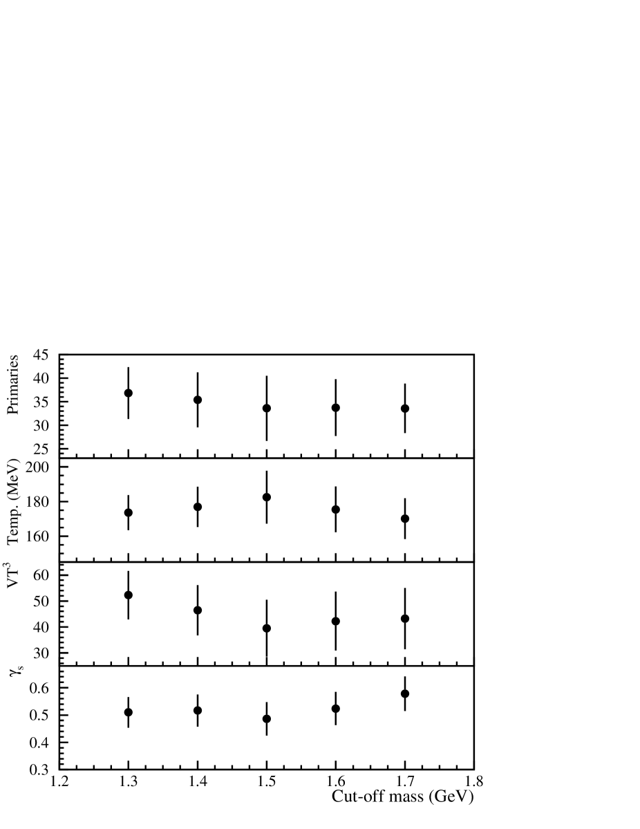
Figure 11:

References

• [1] R. Hagedorn: Suppl. Nuovo Cimento 3 (1965) 147
• [2] R. Hagedorn, in: Hot Hadronic Matter: Theory and Experiment, (J. Letessier et al., eds.), p. 13 (NATO ASI Series, Vol. B346, Plenum, New York, 1995)
• [3] E. Schnedermann, J. Sollfrank, U. Heinz: Phys. Rev. C 48 (1993) 2462
• [4] U. Heinz: Nucl. Phys. A 566 (1994) 225c
• [5] R. Hagedorn, K. Redlich: Z. Phys. C 27 (1985) 541
• [6] W. BlΓΌmel, J. Sollfrank, U. Heinz: Z. Phys. C 63 (1994) 637
W. BlΓΌmel, U. Heinz, Z. Phys. C 67 (1995) 281
• [7] F. Becattini: Z. Phys. C 69 (1996) 485
• [8] F. Becattini: Ph.D. thesis, University of Florence, February 1996 (in italian)
• [9] F. Becattini: Firenze Preprint DFF 262/12/1996, to be published in the proceedings of the XXVI International Symposium on Multiparticle Dynamics, September 1-5 1996, Faro (Portugal)
• [10] For a covariant treatment of thermodynamics see for instance: B. Touschek: Nuovo Cimento B 63 (1968) 295
• [11] K. Redlich, L. Turko: Z. Phys. C 5 (1982) 200
• [12] L. Turko: Phys. Lett. B 104 (1981) 153
• [13] J. Rafelski: Phys. Lett. B 262 (1991) 333
J. Letessier, A. Tounsi, J. Rafelski: Phys. Lett. B 292 (1992) 417
For a formal derivation see: C. Slotta, J. Sollfrank, U. Heinz, in: Strangeness in Hadronic Matter, (J. Rafelski, ed.), American Institute of Physics Conference Proceedings 340 (1995) 462
• [14] For a review, see: M. Basile et al.: Nuovo Cimento A 66, N. 2 (1981) 129
• [15] F. Becattini, A. Giovannini, S. Lupia: Z. Phys. C 72 (1996) 491
• [16] Particle Data Group: Review of Particle Properties, Phys. Rev. D 50 (1994)
• [17] For unknown heavy flavoured hadrons branching ratios we used estimates from the JETSET Monte-Carlo program:
T. SjΓΆstrand: Comp. Phys. Comm. 28 (1983) 229
T. SjΓΆstrand: Pythia 5.7 and. Jetset 7.4, CERN/TH 7112/93 (1993)
• [18] R. Ammar et al., LEBC-MPS Coll.: Phys. Rev. Lett. 61 (1988) 2185
M. Aguilar-Benitez et al., LEBC-EHS Coll.: Z. Phys. C 40 (1998) 321
• [19] M. Aguilar-Benitez et al., LEBC-EHS Coll.: Z. Phys. C 50 (1991) 405
• [20] A. De Angelis: CERN/PPE 95-135
• [21] J. Allday et al., NA5 Coll.: Z. Phys. C 40 (1988) 29
• [22] S. Barish et al.: Phys. Rev. D 9 (1974) 2689
• [23] K. Jaeger et al.: Phys. Rev. D 11 (1975) 2405
• [24] R. Singer et al.: Phys. Lett. B 60 (1975) 385
• [25] T. Kafka et al.: Phys. Rev. D 19 (1979) 76
• [26] U. Amaldi, K. R. Schubert: Nucl. Phys. B 166 (1980) 301
• [27] F. Lo Pinto et al.: Phys. Rev. D 22 (1980) 573
• [28] J. L. Bailly et al., EHS-RCBC Coll.: Z. Phys. C 23 (1984) 205
• [29] M. Asai et al., EHS-RCBC Coll.: Z. Phys. C 27 (1985) 11
• [30] H. Kichimi et al.: Phys. Rev. D 20 (1979) 37
• [31] T. Okuzawa et al.: KEK Preprint KEK-87-146
• [32] R. E. Ansorge et al., UA5 Coll.: Nucl. Phys. B 328 (1989) 36 and references therein
• [33] F. Becattini: Firenze Preprint DFF 263/12/1996 hep-ph 9701275, to be published in the proceedings of the XXXIII Eloisatron workshop ”Universality features of multihadron production and the leading effect”, October 19-25 1996, Erice (Italy)
• [34] J. Cleymans et al.: CERN/TH 95-298
P. Braun-Munziger et al.: Phys. Lett. B 365 (1996) 1
• [35] R. Vogt.: Z. Phys. C 71 (1996) 475
• [36] A. Giovannini, S. Lupia, R. Ugoccioni: Phys. Lett. B 374 (1996) 231
• [37] M. Asai et al., EHS-RCBC Coll.: Z. Phys. C 34 (1987) 429
• [38] E. Laermann, in: Quark Matter β€˜96, (P. Braun-Munzinger et al., eds.), Nucl. Phys. A (1996), in press.
• [39] Thermal analysis in heavy ions collisions found $\gamma_{s}\simeq 1$: J. Sollfrank et al.: Z. Phys. C 61 (1994) 659